Fractional-Order Control of Grid-Connected Photovoltaic System Based on Synergetic and Sliding Mode Controllers

Abstract

Starting with the problem of connecting the photovoltaic (PV) system to the main grid, this article presents the control of a grid-connected PV system using fractional-order (FO) sliding mode control (SMC) and FO-synergetic controllers. The article presents the mathematical model of a PV system connected to the main grid together with the chain of intermediate elements and their control systems. To obtain a control system with superior performance, the robustness and superior performance of an SMC-type controller for the control of the u_dc voltage in the DC intermediate circuit are combined with the advantages provided by the flexibility of using synergetic control for the control of currents i_d and i_q. In addition, these control techniques are suitable for the control of nonlinear systems, and it is not necessary to linearize the controlled system around a static operating point; thus, the control system achieved is robust to parametric variations and provides the required static and dynamic performance. Further, by approaching the synthesis of these controllers using the fractional calculus for integration operators and differentiation operators, this article proposes a control system based on an FO-SMC controller combined with FO-synergetic controllers. The validation of the synthesis of the proposed control system is achieved through numerical simulations performed in Matlab/Simulink and by comparing it with a benchmark for the control of a grid-connected PV system implemented in Matlab/Simulink. Superior results of the proposed control system are obtained compared to other types of control algorithms.

1. Introduction

It is a well-known fact that it is important to use, to an increasing extent, renewable energy, characterized by the fact that it is generated from easily renewable sources which can thus be considered unlimited energy. Among these types of renewable energy sources, we refer to solar energy, wind energy, water energy, geothermal energy, etc. There is also a strong upward trend in the study and use of the PV system technology. Obviously, the study of its control systems was also developed in parallel with it [1].

Moreover, among the general approaches to the study of microgrid systems control, we can mention the study of the transient stability of a hybrid microgrid [2,3], the use of algorithms to offset lagging in the microgrid system [4], the optimization of the charging process of microgrid batteries [5,6], the study of the topologies of the converters used in the microgrid [7], the parallel coupling of the inverters in a microgrid [8], problems related to fault tolerance in the microgrid [9], and also problems related to the multi-grid dispatching in view of obtaining an economic optimum [10,11,12,13,14].

An inherent problem that arises is the control of the process of the PV system connection to a main grid. The components which ensure the connection of the PV system to the main grid are the DC-DC boost converter, the DC intermediate circuit, the DC-AC converter, the filtering block, and the transformer for the connection to the main grid, together with their control systems. Further, a task of maximum importance in terms of the control of the grid-connected PV system is to maintain the DC voltage in the intermediate circuit—DC link voltage—u_dc as precisely as possible. The control of this voltage is performed by a cascade control system in which the outer control loop controls the level of u_dc voltage, and the inner control loops control currents i_d and i_q in the dq rotating reference frame. Usually, the synchronization with the main grid is performed through a phase-locked loop (PLL), and the controllers of the control loops are of the classic proportional integrator (PI) type [15].

In order to obtain a more precise control of the voltage u_dc, we can use more complex control algorithms of the adaptive [16], robust [17,18], and predictive [19] types, but also intelligent control algorithms, such as fuzzy [20], neuro-fuzzy [21], genetics [22], particle swarm optimization (PSO) [23], and reinforcement learning [24].

A type of special controller used for the control of linear and nonlinear systems is based on PI and passivity theory [25]. This type of control, known at the beginning as the hyperstability control theory, is based on the appropriate description of the system in the closed loop in the form of the Lagrangian or the port-controlled Hamiltonian, which defines the behavior of the system through energy functions. This description is generally expressed in the form of solutions to partial differential equations, which require an increased degree of difficulty in the implementation of these types of controllers.

An alternative for the synthesis of some controllers for nonlinear systems, which ensures the parametric robustness and maintains a low order of the synthesized control law, is the use of SMC [26]. Among the disadvantages of the SMC-type control, we mention the occurrence of the chattering phenomenon, which represents the occurrence of oscillations in the control input due to the process of synthesis of the controller. For this purpose, to reduce oscillations, transition functions smoother than the sgn function are used (between conventional thresholds +1 and −1) followed by a corresponding filtration. Further, a type of controller suitable for the control of nonlinear systems is the synergetic controller [27]. It is important to recall that, by using such a controller, it is not necessary to linearize the nonlinear model around a static operating point because this type of controller provides good performance for the entire operating range of the nonlinear model.

By adding the FO calculus and the fractional differentiation and integration operators [28,29], control laws can be obtained with a higher degree of refinement due to the additional control parameter which represents the order of the fractional differentiation and integration operator. Thus, a control structure in which classical PI controllers are replaced with FO-synergetic controllers is presented in [30]. Superior results are obtained by using the control structure proposed in this article, as well as the proposed macro-variables for the synthesis of control laws.

The main contributions of this article consist in replacing the classic PI-type controllers in the control loops of u_dc voltage and i_d and i_q currents with, respectively, the FO-SMC and FO-synergetic type controllers. Thus, the synthesis of the control laws related to these types of controllers is presented, as well as the results obtained by numerical simulations in Matlab/Simulink for the control of the grid-connected PV system, in which classic PI, synergetic, or FO-synergetic controllers are used for the inner control loops of currents i_d and i_q, and classic PI, SMC, or FO-SMC controllers are used for the outer control loop of u_dc. Owing to the levels of freedom and the refinement brought by the fractional calculus for the SMC and synergetic algorithms, the performances of the control system will be superior to those presented in the benchmark implementation in [15] but will also compare to the results obtained in other papers using the basic approach presented in [15].

The main contributions of this paper can be summarized as follows:

• We propose the cascade structure of the control system of the grid-connected PV system based on the robustness of an SMC-type controller for the control of u_dc voltage in the DC intermediate circuit, combined with the flexibility of using synergetic control for the control of currents i_d and i_q.
• The synthesis of the control laws by SMC- and synergetic-type controllers using the fractional calculus for integration operators and differentiation operators.
• We realized the numerical simulations in Matlab/Simulink, and by comparing them with a benchmark for the control of a grid-connected PV system implemented in Matlab/Simulink, superior results of the proposed control system compared to other types of control algorithms are presented.

The other sections of the paper are structured as follows: Section 2 presents a mathematical model of the grid-connected PV system. Section 3 presents the control of the grid-connected PV system using the FO calculus for the SMC controller and synergetic controllers. Section 4 presents the numerical simulations in Matlab/Simulink for the control of the grid-connected PV system using FO-SMC and FO-synergetic controllers and the analysis thereof, and some conclusions are presented in Section 5.

2. Mathematical Model of the Grid-Connected PV System

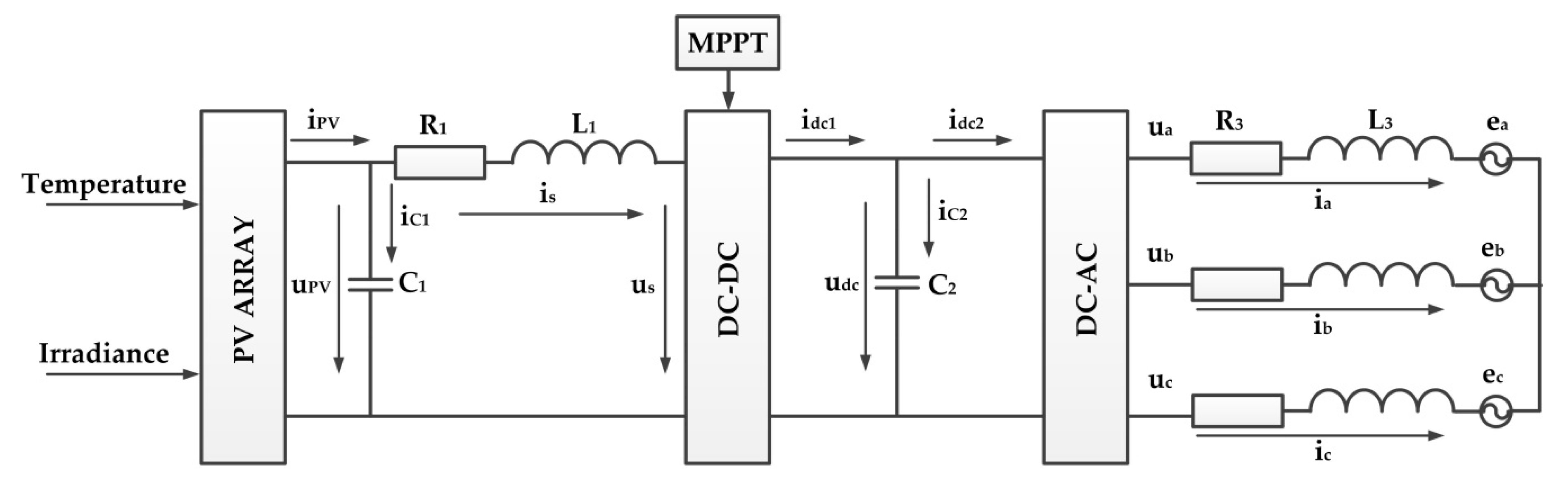
Following [15,27,31], which show the mathematical model of a grid-connected PV system, Figure 1 shows the general diagram of such a system. The PV array system is modeled in [15,27,31] and the input parameters are radiation and temperature. The list of component blocks additionally includes a DC boost converter along with the maximum power point tracking (MPPT) module and a three-phase DC-AC converter. The notations in Figure 1 are the usual ones.

Thus, the following equations can be written to describe the operation of the grid-connected PV system:

$$C_1\frac{d{u}_{PV}}{dt}=i_{PV}-i_s$$

(1)

$$u_{PV}=R{}_{1}i{}_s+L_1\frac{di{}_s}{dt}+u{}_s$$

(2)

$$C_2\frac{d{u}_{dc}}{dt}=i_{dc1}-i_{dc2}$$

(3)

$$u_{abc}-e_{abc}=R{}_{3}i{}_{abc}+L_3\frac{di{}_{abc}}{dt}$$

(4)

where u_abc represents the output voltage of the DC-AC (voltage source converter—VSC) converter with $u_{abc}={\left[\begin{array}{ccc}{u}_a& u_b& u_c\end{array}\right]}^T$, e_abc represents the grid voltage with $e_{abc}={\left[\begin{array}{ccc}{e}_a& e_b& e_c\end{array}\right]}^T$, and i_abc represents the alternating current with $i_{abc}={\left[\begin{array}{ccc}{i}_a& i_b& i_c\end{array}\right]}^T$.

Park’s transformation based on the P matrix is well known:

$$P=\left[\begin{array}{ccc}\sin \left(\omega t\right)& \sin \left(\omega t-\frac{2\pi }{3}\right)& \sin \left(\omega t+\frac{2\pi }{3}\right)\\ \cos \left(\omega t\right)& \cos \left(\omega t-\frac{2\pi }{3}\right)& \cos \left(\omega t+\frac{2\pi }{3}\right)\\ \frac{1}{2}& \frac{1}{2}& \frac{1}{2}\end{array}\right]$$

(5)

By applying this transformation to the abc reference system, we obtain the usual quantities in Figure 1 in the dq reference system (u_dq0 = Pu_abc, e_dq0 = Pe_abc, i_dq0 = Pi_abc). Thus, Equation (4) becomes

$$u_{dq0}-e_{dq0}=R_3{i}_{dq0}+L_3\frac{d{i}_{dq0}}{dt}+L_3\left[\begin{array}{c}-\omega i_q\\ \omega i_d\\ 0\end{array}\right]$$

(6)

By components, this equation can be rewritten in the form of Equations (7) and (8):

$$L_3\frac{d{i}_d}{dt}=-R_3{i}_d+\omega L_3{i}_q-e_d+u_d=u_{3d}+u_d$$

(7)

$$L_3\frac{d{i}_q}{dt}=-R_3{i}_q-\omega L_3{i}_d-e_d+u_q=u_{3q}+u_q$$

(8)

where u_id and u_iq represent the control variables for the command of the DC-AC converter (which is of voltage source converter—VSC-type). Equations (7) and (8) include the following notations: $u_{3d}=-R_3{i}_d+\omega L_3{i}_q-e_d$ and $u_{3q}=-R_3{i}_q-\omega L_3{i}_d-e_q$.

The MPPT algorithm is presented in [15,26,29]; it will provide the duty cycle signal (D) to control the DC boost converter. Thus, the following relations can be written:

$$i_{dc1}=\left(1-D\right)i_s$$

(9)

$$u_s=\left(1-D\right)u_{dc}$$

(10)

3. Control of the Grid-Connected PV System

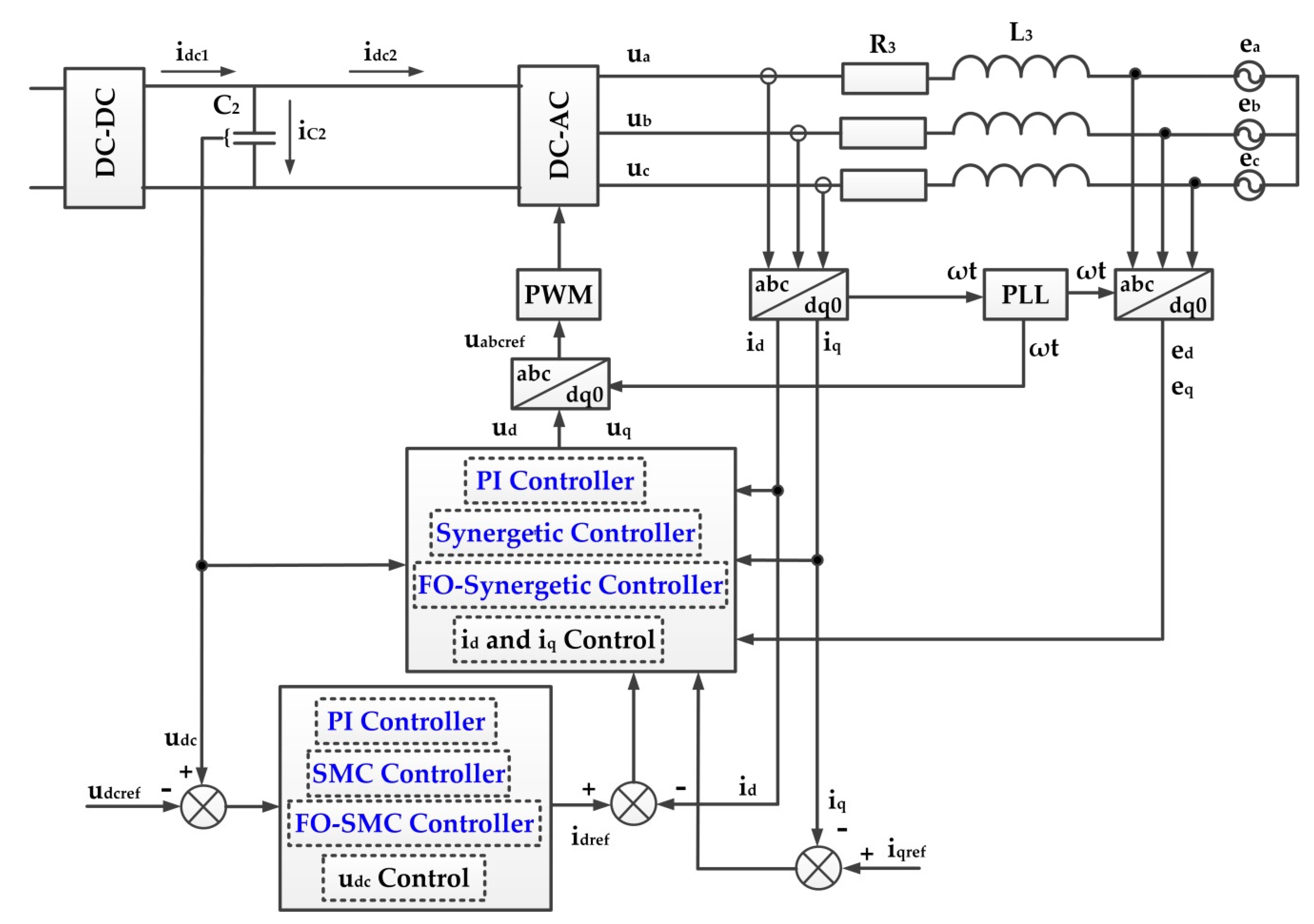
The control of a grid-connected PV system is presented at length in [15,27,31], both in normal operation and in low-voltage ride through (LVRT). The controllers used for the inner control loops of currents i_d and i_q are of the classic PI type or synergetic type [27], while the controller for the outer control loop of u_dc is of the classic PI type [15,31]. Figure 2 shows the control scheme for the connection of a PV system to the power grid under normal operation. The control loops of currents i_d and i_q and of u_dc are presented schematically in Figure 3. In this section, we will present several basic elements of the FO calculus to synthesize the fractional-type control laws in the case of using the design and synthesis procedures of the SMC and synergetic controllers.

3.1. Notions and Notations for Fractional-Order Calculus

To achieve a refinement of the differential and integral calculus, the non-integer order operator is added as $a{D}_t^{\alpha }$, where the FO is noted with α, and the limits of the use of the operator are denoted a and t [28,29].

$$a{D}_t^{\alpha }=\{\begin{array}{c}\frac{d^{\alpha }}{d{t}^{\alpha }} \mathrm{Re}(\alpha )>0\\ 1 \mathrm{Re}(\alpha )=0\\ {\displaystyle {\int }_a^t{(dt)}^{-\alpha } \mathrm{Re}(\alpha )<0}\end{array}$$

(11)

Further, a common alternative definition is given by the Riemann–Liouville differintegral [28,29]:

$$a{D}_t^{\alpha }f\left(t\right)=\frac{1}{\Gamma \left(m-\alpha \right)}{\left(\frac{d}{dt}\right)}^m{\displaystyle \underset{\alpha }{\overset{t}{\int }}\frac{f\left(\tau \right)}{{\left(t-\tau \right)}^{\alpha -m+1}}d\tau }$$

(12)

where $m-1<\alpha <m, m\in N$, and $\Gamma (\cdot )$ is Euler’s gamma function.

For the practical implementation by numerical calculation, the Grünwald–Letnikov definition is presented as follows [28,29]:

$$a{D}_t^{\alpha }f(t)=\underset{h\to 0}{\lim }\frac{1}{h^{\alpha }}{\displaystyle \sum _{j=0}^{\left(\frac{t-\alpha }{h}\right)}{\left(-1\right)}^j}\left(\begin{array}{c}\alpha \\ j\end{array}\right)f\left(t-jh\right)$$

(13)

where (·) is the integer part.

The Laplace transform can also be applied in the non-integer case similarly to the integer case (in terms of the power of the complex operator s). A special case is when the power α of operator s is of the commensurate order type $q, \left(q\in R^{+}, 0<q<1, {\alpha }_k=kq\right)$. For $\lambda =s^q$, the transfer function $H(\lambda )$ can be written as

$$H\left(\lambda \right)=\frac{{\displaystyle \sum _{k=0}^m{b}_k{\lambda }^k}}{{\displaystyle \sum _{k=0}^n{a}_k{\lambda }^k}}$$

(14)

For the numerical implementations in embedded systems in real time, it is important to emphasize that the results of the fractional calculus cannot be implemented directly, but an integer-order approximation of these calculi is used on a specified frequency range $\left({\omega }_b,{\omega }_h\right)$, by using Oustaloup recursive filters.

For $s^{\gamma }$ with $0<\gamma <1$, an approximation can be used as follows [28,29]:

$$G_f\left(s\right)=K{\displaystyle \prod _{k=-N}^N\frac{s+{\omega }_k^{’}}{s+{\omega }_k}}$$

(15)

where ${\omega }_k^{’}$, ${\omega }_k$, and K are given by

$${\omega }_k^{’}={\omega }_b{\left(\frac{{\omega }_h}{{\omega }_b}\right)}^{\frac{k+N+\frac{1}{2}\left(1-\gamma \right)}{2N+1}}; {\omega }_k={\omega }_b{\left(\frac{{\omega }_h}{{\omega }_b}\right)}^{\frac{k+N+\frac{1}{2}\left(1+\gamma \right)}{2N+1}}; k={\omega }_h^{\gamma }$$

(16)

A refined form of Oustaloup-type filters is given by the following relations [28]:

$$s^{\alpha }\approx {\left(\frac{d{\omega }_h}{b}\right)}^{\alpha }\left(\frac{d{s}^2+b{\omega }_{h}s}{d(1-\alpha )s^2+b{\omega }_{h}s+d\alpha }\right)G_p$$

(17)

$$G_p=K{\displaystyle \prod _{k=-N}^N\frac{s+{\omega }_k^{’}}{s+{\omega }_k}}; {\omega }_k={\left(\frac{b{\omega }_h}{d}\right)}^{\frac{\alpha +2k}{2N+1}}; {\omega }_k^{’}={\left(\frac{d{\omega }_b}{b}\right)}^{\frac{\alpha -2k}{2N+1}}$$

(18)

where usually parameters b = 10 and d = 9.

3.2. Fractional-Order Sliding Mode Control

Starting from Equation (3) and using S_a, S_b, and S_c to denote the switching function for the DC-AC converter in Figure 1, the following equation is obtained in the abc frame:

$$C_2\frac{d{u}_{dc}}{dt}=i_{dc1}-\left(i{}_{a}S{}_a+i{}_{b}S{}_b+i{}_{c}S{}_c\right)$$

(19)

The switching functions Sd and S_q can be obtained by using transformation (5):

$${\left[\begin{array}{ccc}{S}_d& S_q& 0\end{array}\right]}^T=P{\left[\begin{array}{ccc}{S}_a& S_b& S_c\end{array}\right]}^T$$

(20)

Based on these, Equation (19) becomes

$$C_2\frac{d{u}_{dc}}{dt}=i_{dc1}-\frac{3}{2}\left(i{}_{d}S{}_d+i{}_{q}S{}_q\right)$$

(21)

In Equation (21), i_dc1 is given by the relations (9) and (10) which depend on the DC boost converter and the MPPT algorithm, which we will consider as an optimized form given by [15,31], so we will consider that it is necessary for the other terms of the right member to be calculated by the sliding mode control technique to maintain u_dc at a prescribed value u_dcref (which is considered constant or has slow variations relative to the variation of the other quantities in the control system). Additionally, in [26], it is demonstrated that, when the three-phase grid system is symmetrical, i_d represents the direct current and reference i_qref = 0 is selected, and thus Equation (21) becomes:

$$C_2\frac{d{u}_{dc}}{dt}=i_{dc1}-\frac{3}{2}i{}_{dref}S{}_d$$

(22)

Following the sliding mode control design procedure, the reference i_dref for the inner control loop of currents i_d and i_q will be determined. Thus, we define the state variable x₁ as

$$x_1=u_{dc}-u_{dcref}$$

(23)

We define the switching surface S:

$$\{\begin{array}{c}S=c_1{x}_1+x_2\\ \dot{S}=c_1{x}_2+{\dot{x}}_2\end{array}$$

(24)

where the state variable x₂ is defined by:

$$x_2={\dot{x}}_1=-{\dot{u}}_{dc}$$

(25)

To achieve convergence, the following is required:

$$\dot{S}=-\epsilon \mathrm{sgn}S-kS$$

(26)

where ε and k are positive constants.

From the calculation, we obtain:

$${\ddot{x}}_1={\dot{x}}_2=-{\ddot{u}}_{dc}=\frac{3}{2}\frac{S_d}{C_2}{\dot{i}}_{dref}-\frac{{\dot{i}}_{dc1}}{C_2},$$

(27)

and thus the following can be written:

$$-\epsilon \mathrm{sgn}S-kS=c_1{x}_2+\frac{3}{2}\frac{1}{C_2}{S}_d{\dot{i}}_{dref}-\frac{{\dot{i}}_{dc1}}{C_2}$$

(28)

Following [32], to improve convergence and reduce high-frequency oscillations, the sgn function is replaced with the function below:

$$h(x)=\frac{2}{1+e^{-a(x-b)}}-1$$

(29)

For a = 4 and b = 0, $h\in [-1 1]$, and a smoothed transition is achieved between −1 and 1. From this, the output of the SMC-type controller can be inferred:

$$i_{dref}=\frac{2}{3}\frac{C_2}{S_d}{\displaystyle \underset{0}{\overset{t}{\int }}\left[-\left(c_1{x}_2+kS-\epsilon h(S)\right)+\frac{{\dot{i}}_{dc1}}{C_2}\right]}dt$$

(30)

For the fractional case, the switching surface is defined as:

$$S=c_1{x}_1+c_2{D}^{\mu }{x}_1=c_1{x}_1+c_2{D}^{\mu -1}{x}_2,$$

(31)

where the fractional differential operator D is defined in relation (11).

By calculating $\dot{S}$, we obtain:

$$\dot{S}=c_1{\dot{x}}_1+c_2{D}^{\mu +1}{x}_1=c_1{x}_2+c_2{D}^{\mu -1}{\dot{x}}_2,$$

(32)

which can be rewritten using Equation (27):

$$\dot{S}=c_1{x}_2+c_2{D}^{\mu -1}\left(\frac{3}{2}\frac{1}{C_2}{S}_d{\dot{i}}_{dref}-\frac{{\dot{i}}_{dc1}}{C_2}\right)$$

(33)

Using Equation (26), we obtain:

$$-\epsilon h(S)-kS-c_1{x}_2=c_2{D}^{\mu -1}\left(\frac{3}{2}\frac{1}{C_2}{S}_d{\dot{i}}_{dref}-\frac{{\dot{i}}_{dc1}}{C_2}\right)$$

(34)

By applying operator $D^{1-\mu }$ to relation (34), we obtain:

$$D^{1-\mu }\left(-\epsilon h(S)-kS-c_1{x}_2\right)=c_2\frac{3}{2}\frac{1}{C_2}{S}_d{\dot{i}}_{dref}-c_2\frac{{\dot{i}}_{dc1}}{C_2}$$

(35)

The output of the FO-SMC type controller can thus be inferred from the following:

$$i_{dref}=\frac{2}{3c_2}\frac{C_2}{S_d}{\displaystyle \underset{0}{\overset{t}{\int }}\left[c_2\frac{{\dot{i}}_{dc1}}{C_2}+D^{1-\mu }\left(-\epsilon h(S)-kS-c_1{x}_2\right)\right]dt}$$

(36)

Both in Equation (30) and in Equation (36), in order to avoid the uncontrolled increase in i_dref due to the zero-crossings of the signal S_d, it will be replaced in the practical implementation with $S_d^{’}=S_d+c_3,$ where $c_3>0$ becomes a new level of freedom in the design of the FO-SMC controller.

3.3. Fractional-Order Synergetic Control

It is well known that synergetic control can be considered as a generalization of sliding mode control. Thus, synergetic control can be applied to nonlinear systems described by the general form [27,32]

$$\dot{x}=f\left(x,u,t\right)$$

(37)

where x represents the state vector, $x\in {\Re }^n$; $f(.)$ represents the continuous nonlinear function; u represents the control vector, $u\in {\Re }^m, \left(m<n\right)$.

The synergetic control procedure includes the selection of a macrovariable $\psi \left(x,t\right)$ which depends on the states of the system, for each control input. The system will be forced to evolve to manifolds $\psi =0$, according to the following equation:

$$T\dot{\psi }+\psi =0$$

(38)

where T > 0 is selected to obtain the desired convergence rate.

By differentiating the macrovariable Ψ, we obtain:

$$\dot{\psi }=\frac{\partial \psi }{\partial x}\dot{x},$$

(39)

and by inserting the relation (39) into Equation (38), we obtain:

$$T\frac{\partial \psi }{\partial x}\dot{x}+\psi =0$$

(40)

The explicit forms of $\dot{x}$ states in the mathematical model of the controlled system are inserted into Equation (40). This results in the control law as follows:

$$u=u\left(x,\psi (x,t),T,t\right)$$

(41)

Next, we will apply the integer-order and fractional-order synergetic control procedures to replace the classic PI-type control loops of currents i_d and i_q. The outputs of the synergetic controller will be u_d and u_q (see Figure 2).

For the d-axis, for k_d > 0, we choose the macrovariable Ψ_d as follows:

$${\psi }_d=\left(u_{dcref}-u_{dc}\right)+k_d\left(i_{dref}-i_d\right)$$

(42)

We define another state variable x₂ (in addition to the state variable x₁ in Equation (23)):

$$\{\begin{array}{c}x{}_1=u_{dcref}-u_{dc}\\ x{}_2=i_{dref}-i_d\end{array}$$

(43)

Based on the relation (43) for slow variations of the reference quantities or quasi-stationary regime, the following relation can be written:

$$\{\begin{array}{c}\dot{x}{}_1=-{\dot{u}}_{dc}\\ \dot{x}{}_2=-{\dot{i}}_d\end{array}$$

(44)

Using these, we obtain the macrovariable derivative Ψ_d defined in relation (42), of the following form:

$${\dot{\psi }}_d=\dot{x}{}_1+k_d\dot{x}{}_2=-{\dot{u}}_{dc}-k_d{\dot{i}}_d$$

(45)

Based on these, for T = T₁, Equation (40) becomes:

$$T_1\left(-{\dot{u}}_{dc}-k_d{\dot{i}}_d\right)+\left(u_{dcref}-u_{dc}\right)+k_d\left(i_{dref}-i_d\right)=0$$

(46)

Using Equation (7), Equation (46) becomes:

$$-T_1{\dot{u}}_{dc}-T_1{k}_d\frac{1}{L_3}\left(u_{3d}-u_d\right)+\left(u_{dcref}-u_{dc}\right)+k_d\left(i_{dref}-i_d\right)=0$$

(47)

After rearranging the terms in Equation (47), we can write:

$$T_1{k}_d\frac{1}{L_3}{u}_d=-T_1{\dot{u}}_{dc}-T_1{k}_d\frac{1}{L_3}{u}_{3d}+\left(u_{dcref}-u_{dc}\right)+k_d\left(i_{dref}-i_d\right)$$

(48)

Based on this, we obtain the control law u_d as follows:

$$u_d=\frac{L_3}{T_1{k}_d}\left[-T_1{\dot{u}}_{dc}-T_1{k}_d\frac{1}{L_3}{u}_{3d}+\left(u_{dcref}-u_{dc}\right)+k_d\left(i_{dref}-i_d\right)\right]$$

(49)

For axis d in the fractional case, the macrovariable is chosen:

$${\psi }_d=D^{\mu }{x}_1+k_d{x}_2$$

(50)

By deriving Equation (50), we obtain:

$${\dot{\psi }}_d=D^{\mu }{\dot{x}}_1+k_d{\dot{x}}_2=-D^{\mu }{\dot{u}}_{dc}-k_d{\dot{i}}_d$$

(51)

Based on these, Equation (40) becomes

$$T_1\left(-D^{\mu }{\dot{u}}_{dc}-k_d{\dot{i}}_d\right)+D^{\mu }\left(u_{dcref}-u_{dc}\right)+k_d\left(i_{dref}-i_d\right)=0$$

(52)

Using Equation (7), Equation (52) becomes:

$$-T_1{D}^{\mu +1}{u}_{dc}-T_1{k}_d\frac{1}{L_3}\left(u_{3d}+u_d\right)+D^{\mu }\left(u_{dcref}-u_{dc}\right)+k_d\left(i_{dref}-i_d\right)=0$$

(53)

After rearranging the terms in Equation (53), we can write:

$$T_1{k}_d\frac{1}{L_3}{u}_d=-T_1{D}^{\mu +1}{u}_{dc}-T_1{k}_d\frac{1}{L_3}{u}_{3d}+D^{\mu }\left(u_{dcref}-u_{dc}\right)+k_d\left(i_{dref}-i_d\right)$$

(54)

Based on this, we obtain the control law u_d as follows:

$$u_d=\frac{L_3}{T_1{k}_d}\left[-T_d{D}^{\mu +1}{u}_{dc}-T_1{k}_d\frac{1}{L_3}{u}_{3d}+D^{\mu }\left(u_{dcref}-u_{dc}\right)+k_d\left(i_{dref}-i_d\right)\right]$$

(55)

For the q-axis, for k_q > 0, we choose the macrovariable Ψ_q of the following form:

$${\psi }_q=i_{qref}-i_q$$

(56)

We define another state variable x₃ (in addition to the state variables x₁ and x₂ in Equation (43)):

$$\{\begin{array}{c}x{}_1=u_{dcref}-u_{dc}\\ \begin{array}{l}x{}_2=i_{dref}-i_d\\ x_3=i_{qref}-i_q\end{array}\end{array}$$

(57)

Based on relation (57), because i_qref is set to zero, we can write:

$$\{\begin{array}{c}\dot{x}{}_1=-{\dot{u}}_{dc}\\ \begin{array}{l}\dot{x}{}_2=-{\dot{i}}_d\\ {\dot{x}}_3=-{\dot{i}}_q\end{array}\end{array}$$

(58)

Using these, we obtain the macrovariable derivative Ψ_q defined in relation (56), of the following form:

$${\dot{\psi }}_q={\dot{x}}_3$$

(59)

Based on these, for T = T₂, Equation (40) becomes:

$$-T_2{\dot{i}}_q+\left(i_{qref}-i_q\right)=0$$

(60)

Using Equation (8), Equation (60) becomes:

$$-T_2\frac{1}{L_3}\left(u_{3q}+u_q\right)+i_{qref}-i_q=0$$

(61)

After rearranging the terms in Equation (61), we can write:

$$\left(u_{3q}+u_q\right)=\frac{L_3}{T_2}\left(i_{qref}-i_q\right)$$

(62)

Based on this, we obtain the control law u_q as follows:

$$u_q=\frac{L_3}{T_2}\left(i_{qref}-i_q\right)-u_{3q}$$

(63)

For the q-axis in the fractional case, the macrovariable is chosen:

$${\psi }_q=D^{\mu }{x}_3+k_q{\displaystyle \underset{0}{\overset{t}{\int }}{x}_3(t)dt}$$

(64)

By deriving Equation (64), we obtain:

$${\dot{\psi }}_q=D^{\mu }{\dot{x}}_3+k_q{x}_3=-D^{\mu }{\dot{i}}_q+k_q\left(i_{qref}-i_q\right)$$

(65)

Based on these, Equation (40) becomes:

$$T_2\left[D^{\mu }\left(-\frac{1}{L_3}\left(u_{3q}+u_q\right)\right)+k_q\left(i_{qref}-i_q\right)\right]+D^{\mu }\left(i_{qref}-i_q\right)+k_q{\displaystyle \underset{0}{\overset{t}{\int }}\left(i_{qref}-i_q\right)dt}=0$$

(66)

By using Equation (8) and applying the fractional operator defined in relation (11) to both members of Equation (66), and considering that $D^{-\mu }$ becomes $I_{\mu }$, we can write:

$$-\frac{T_2}{L_3}\left(u_{3q}+u_q\right)+T_2{k}_q{I}_{\mu }\left(i_{qref}-i_q\right)+\left(i_{qref}-i_q\right)+k_q{I}_{\mu +1}\left(i_{qref}-i_q\right)=0$$

(67)

After rearranging the terms in Equation (67), we can write:

$$\frac{T_2}{L_3}{u}_q=T_q{k}_q{I}_{\mu }\left(i_{qref}-i_q\right)+\left(i_{qref}-i_q\right)+k_q{I}_{\mu +1}\left(i_{qref}-i_q\right)-\frac{T_2}{L_3}{u}_{3q}$$

(68)

Based on this, we obtain the control law u_q as follows:

$$u_q=\frac{L_3}{T_2}\left[T_2{k}_q{I}_{\mu }\left(i_{qref}-i_q\right)+\left(i_{qref}-i_q\right)+k_q{I}_{\mu +1}\left(i_{qref}-i_q\right)-\frac{T_2}{L_3}{u}_{3q}\right]$$

(69)

In the case of integer-order synergetic control, the control inputs u_d and u_q are provided by Equations (49) and (63), and in the case of the fractional synergetic control, the control inputs u_d and u_q are provided by Equations (55) and (69). By applying the inverse Park transform, the actual control inputs u_abc (see Figure 2) are obtained as follows:

$$u_{abc}=P^{-1}{u}_{dq0}$$

(70)

4. Numerical Simulations and Analysis for the Control of the Grid-Connected PV System Using FO-SMC and FO-Synergetic Controllers

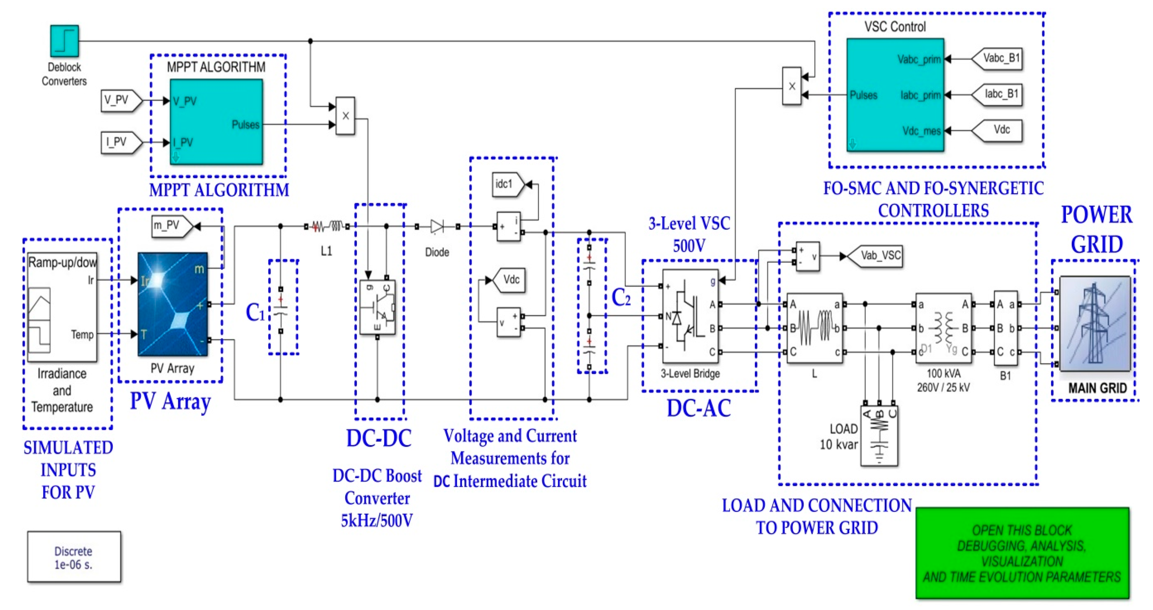
In this section, starting from the controllers synthesized in the previous section, we will present the obtained results of the global system for the control of the grid-connected PV system, in which classic PI, synergetic, or FO-synergetic controllers are used for the inner control loops of currents i_d and i_q and classic PI, SMC, or FO-SMC controllers are used for the outer control loop of u_dc. Owing to the levels of freedom and the refinement brought by the fractional calculus for the SMC and synergetic algorithms, it will be demonstrated, through numerical simulations, using the Matlab/Simulink environment, that superior performance is achieved using the proposed control system. The system described in Figure 2 and Figure 3 is implemented in Matlab/Simulink and the block diagram is presented in Figure 4.

The presented implementation starts from an example in Matlab/Simulink [15], which presents the control system and the performances for a 100 kW model of the grid-connected PV array. The reference value of the voltage in the DC intermediate circuit is set to 500 V and the rated AC voltage supplied by the DC-AC converter is of 260 V. Further, the load is connected to the main grid through a distribution transformer with a rated voltage of 25 kV/260 V. The MPPT algorithm and its performances are presented and implemented in [15,31] and are used in the implementation presented in this article as a block function.

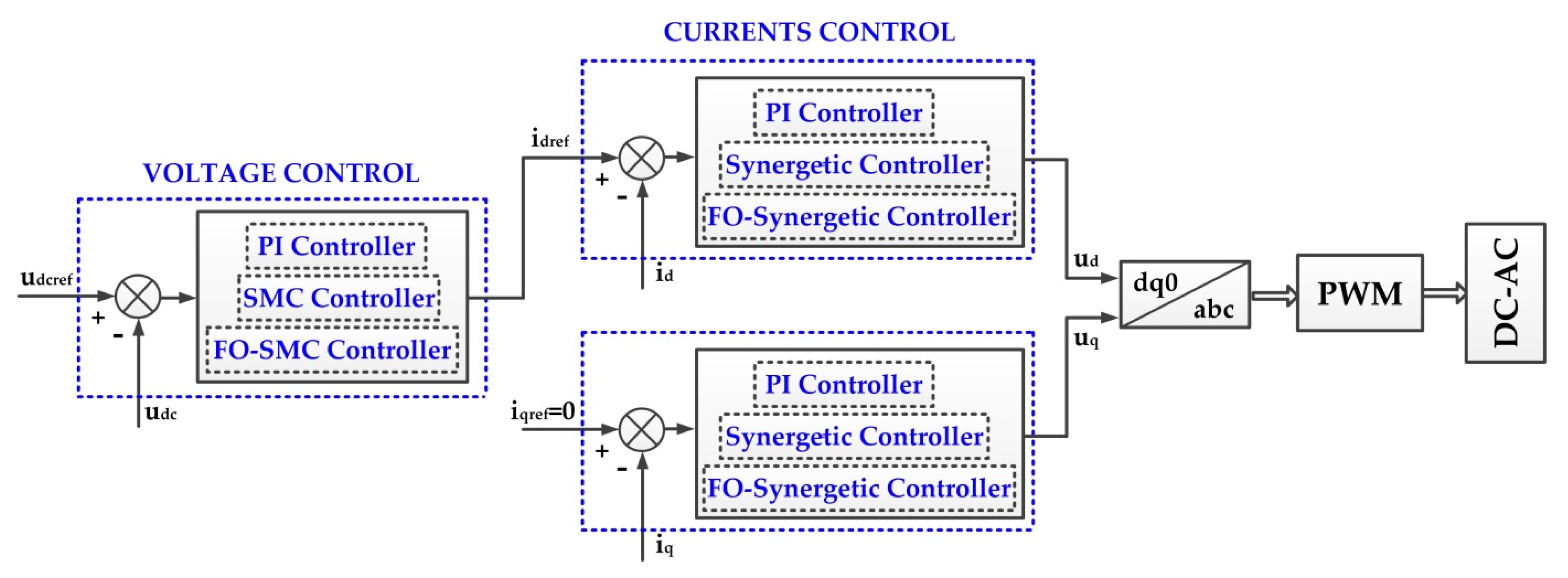
In order to have the smallest possible fluctuations when the DC-AC converter supplies a variable load, the importance of the precise control of the voltage level in the DC intermediate circuit—u_dc—is well known. For this, two cascade control loops are used, an outer one for the control of u_dc and two inner loops for the control of currents i_d and i_q. The current reference and i_dref are supplied by the output of the outer loop controller, and i_qref is set to zero [26].

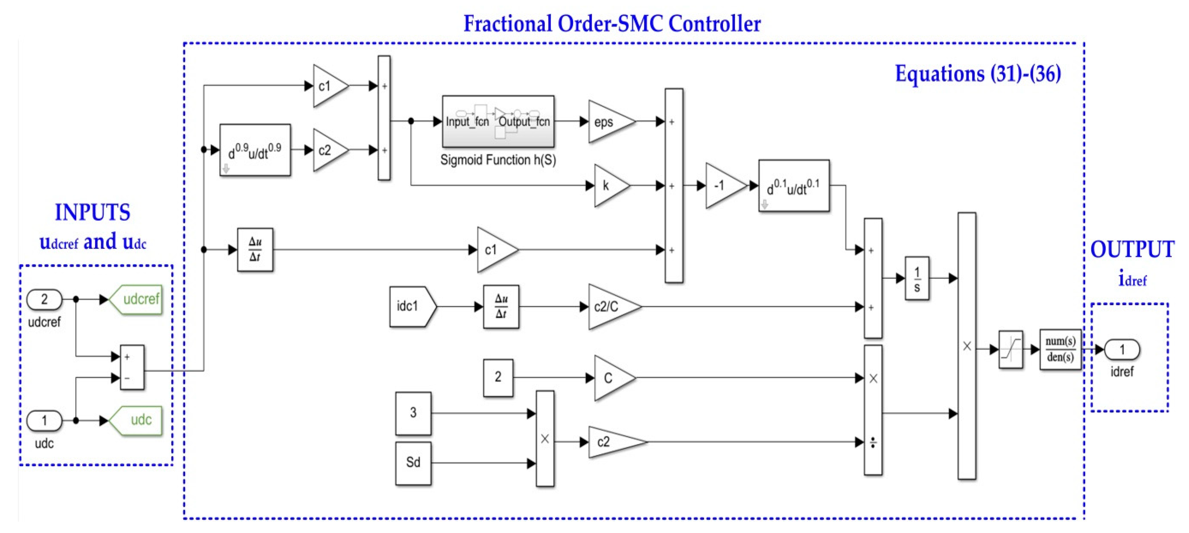
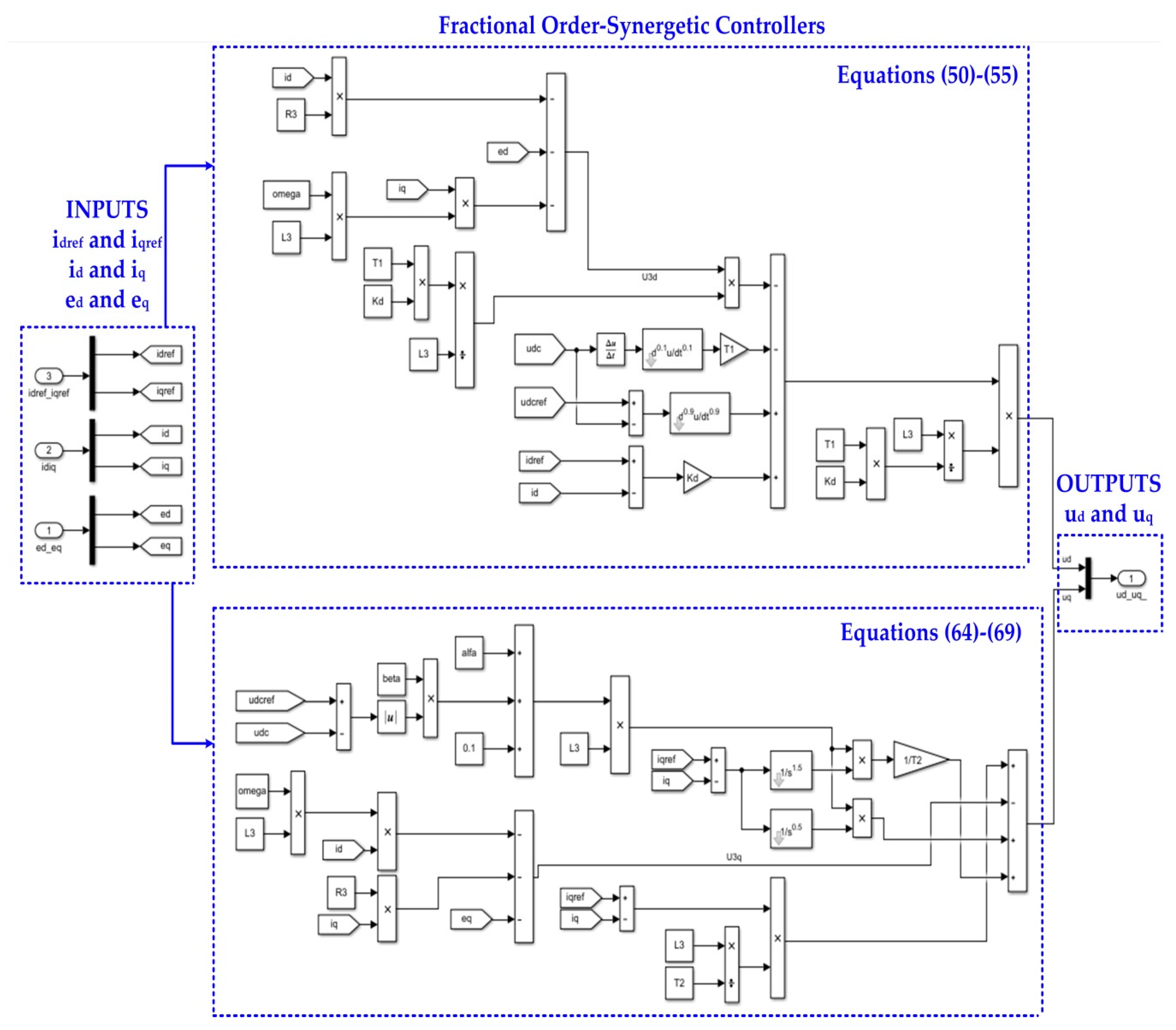
Figure 5 and Figure 6 show the Matlab/Simulink implementations of the control laws synthesized in Section 3 for the most complex case, where the controller of the outer control loop of voltage u_dc is of the FO-SMC type, and the inner control loops of currents i_d and i_q are of the FO-synergetic type. Moreover, in Figure 4, the signal filtering at the DC-AC converter output is achieved using a 10 kvar bank capacitor, which can be considered as the load for the control system.

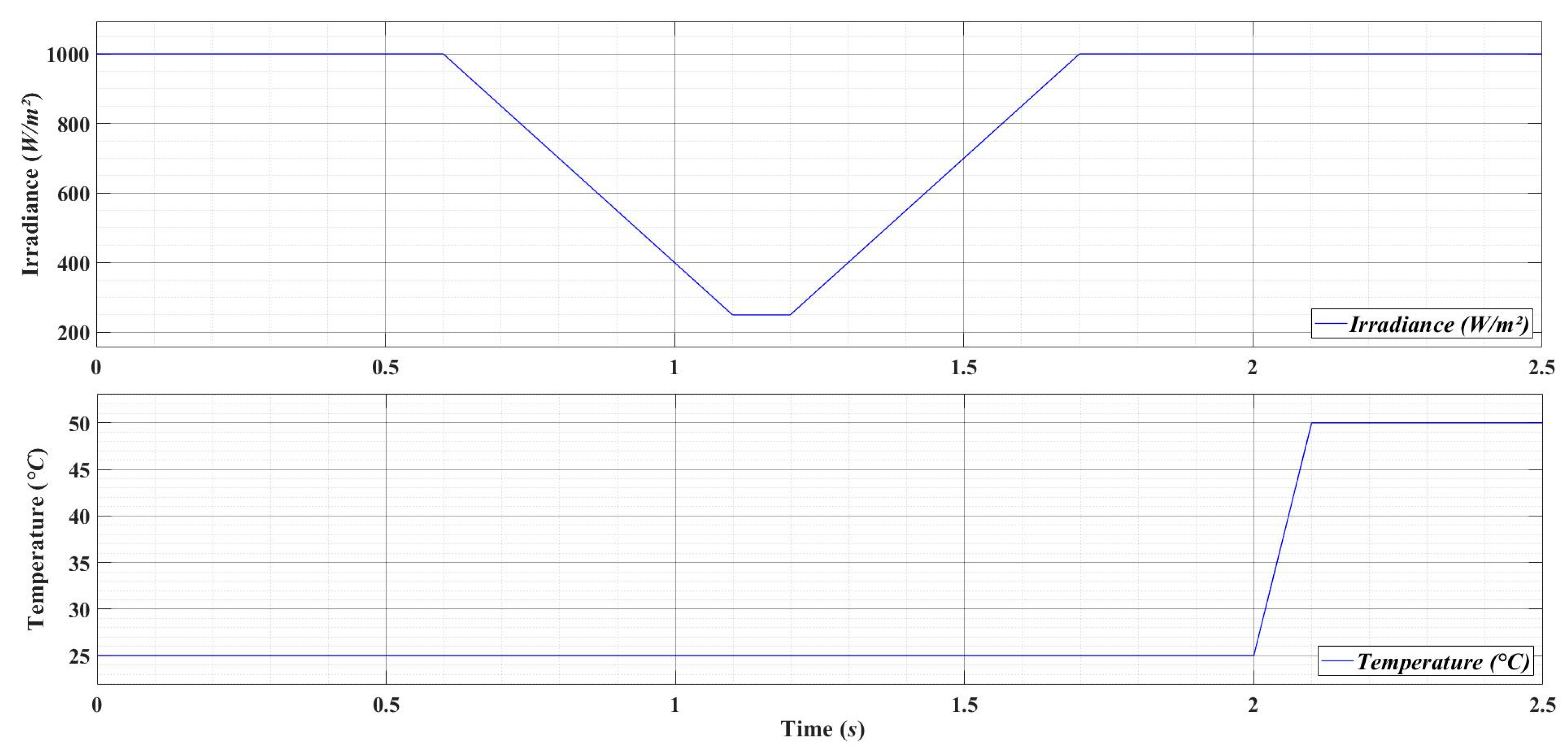
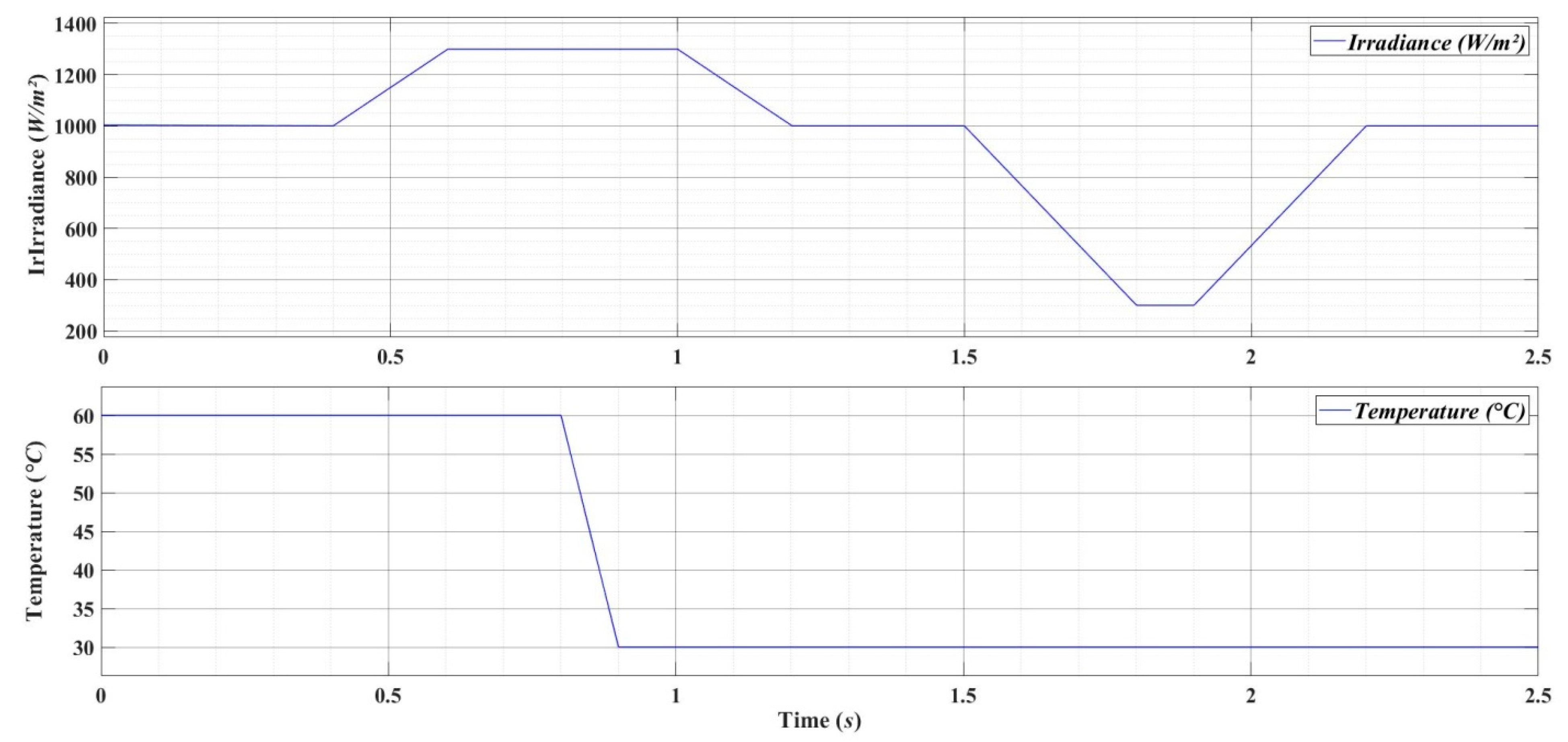
The operation of the PV array is also implemented in [15], and the time variation of the irradiance and temperature input signals is shown in Figure 7. The PV array includes 330 SunPower-type modules which can supply a maximum of 100.7 kW (305.2 W/modules), and each module is characterized by an open-circuit voltage of V_oc = 64.2 V and a short-circuit current of I_sc = 5.96 A. In the Matlab/Simulink implementation, the sample time used is of one microsecond for the Pulse Width Modulation (PWM) generator command signals for the DC-DC and DC-AC converters. For the control system of the voltage and currents, but also for the PLL-type synchronization loop, the sampling period is of 0.1 ms.

In the Matlab/Simulink implementation in [15], for the first 50 ms, the operation of the converters is bypassed during the period when the control system operates in the open loop. After the first 50 ms, the controllers come into operation both for the DC-DC converter and for the MPPT algorithm provided by [31], but also for the control of the DC-AC converter whose improved FO-SMC and FO-synergetic controllers proposed in this article provide superior performance compared to the classical PI controllers proposed in [15], both in stationary mode and in dynamic mode (see Figure 8, Figure 9, Figure 10 and Figure 11).

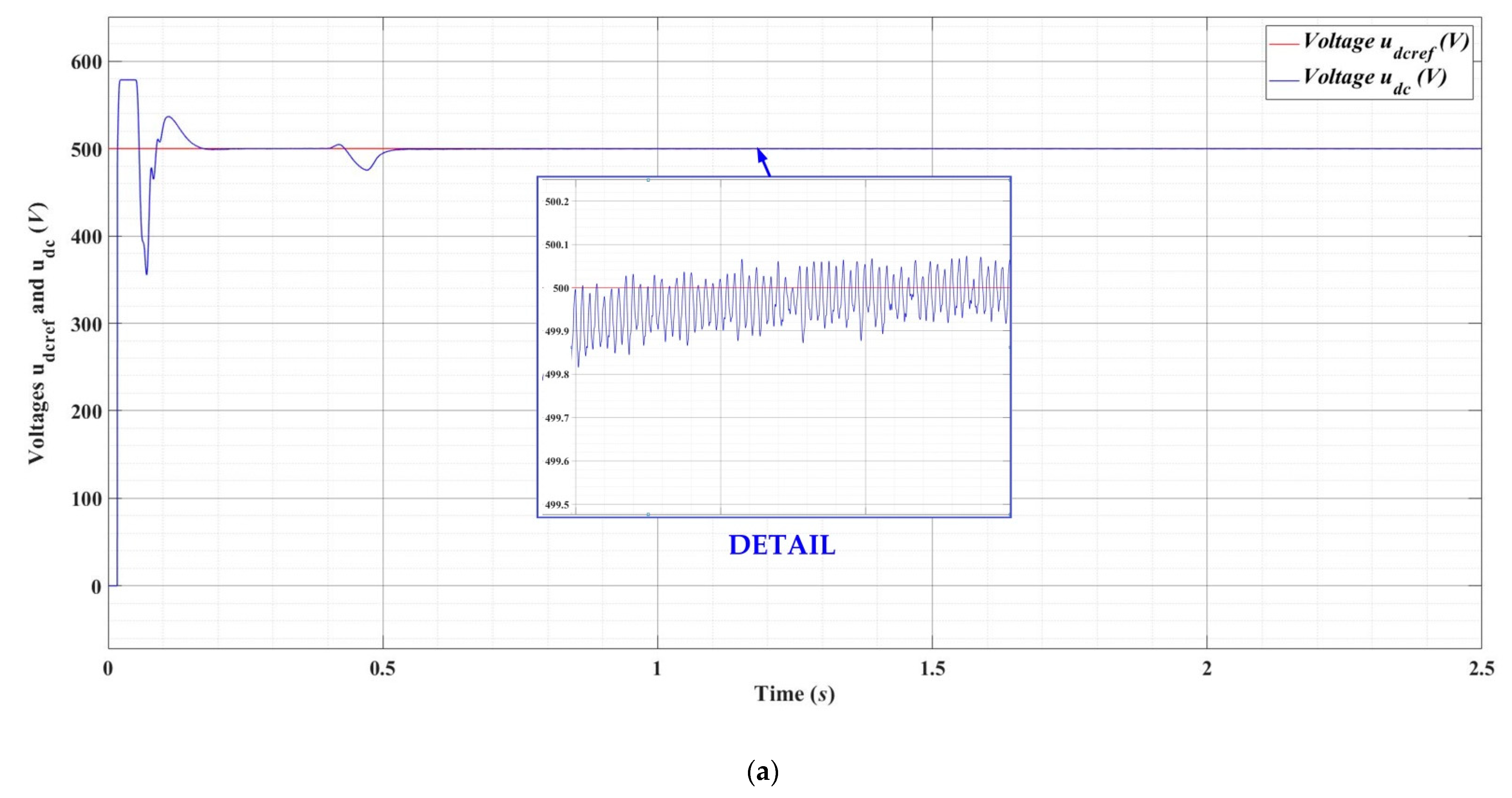
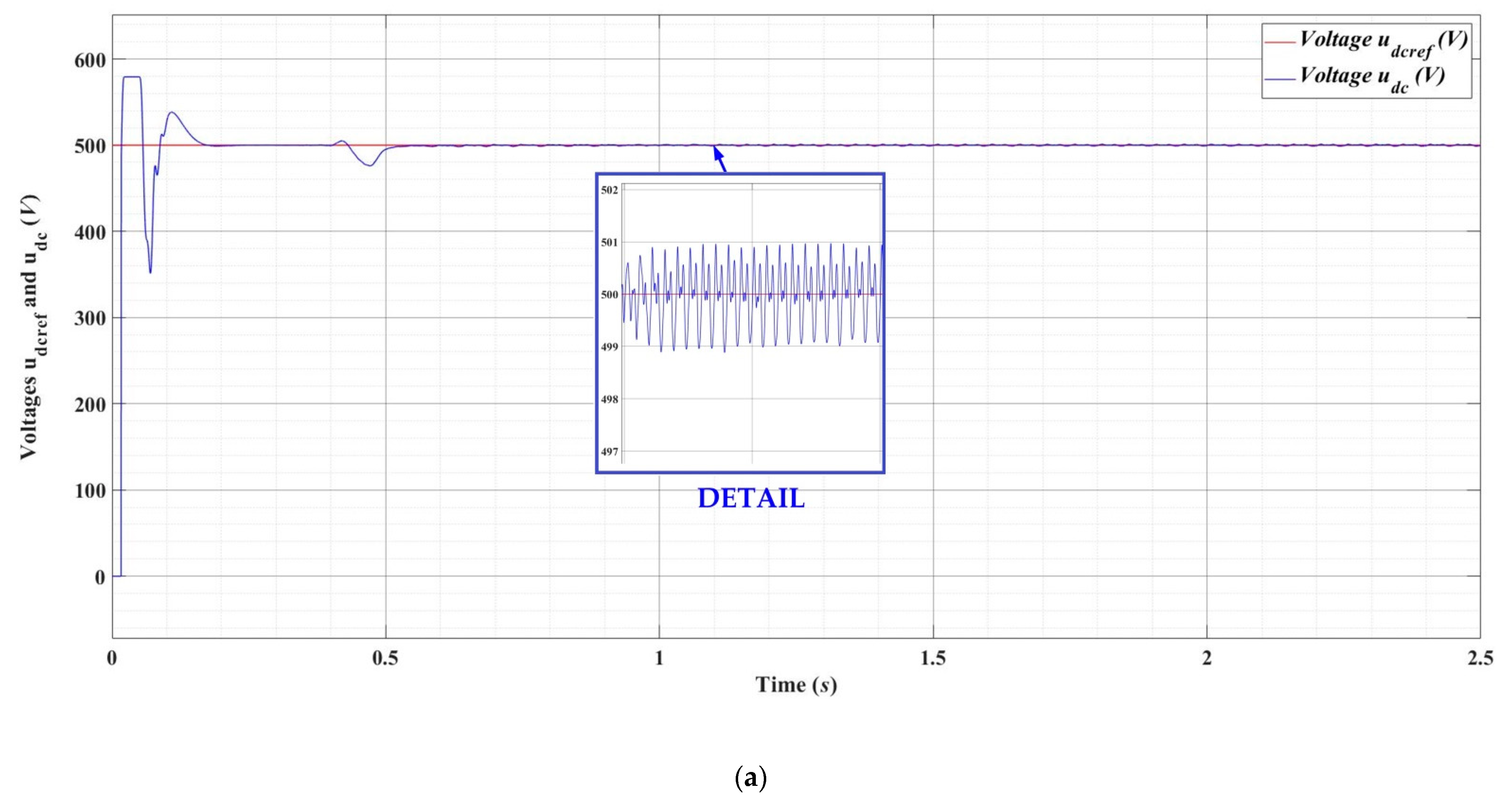
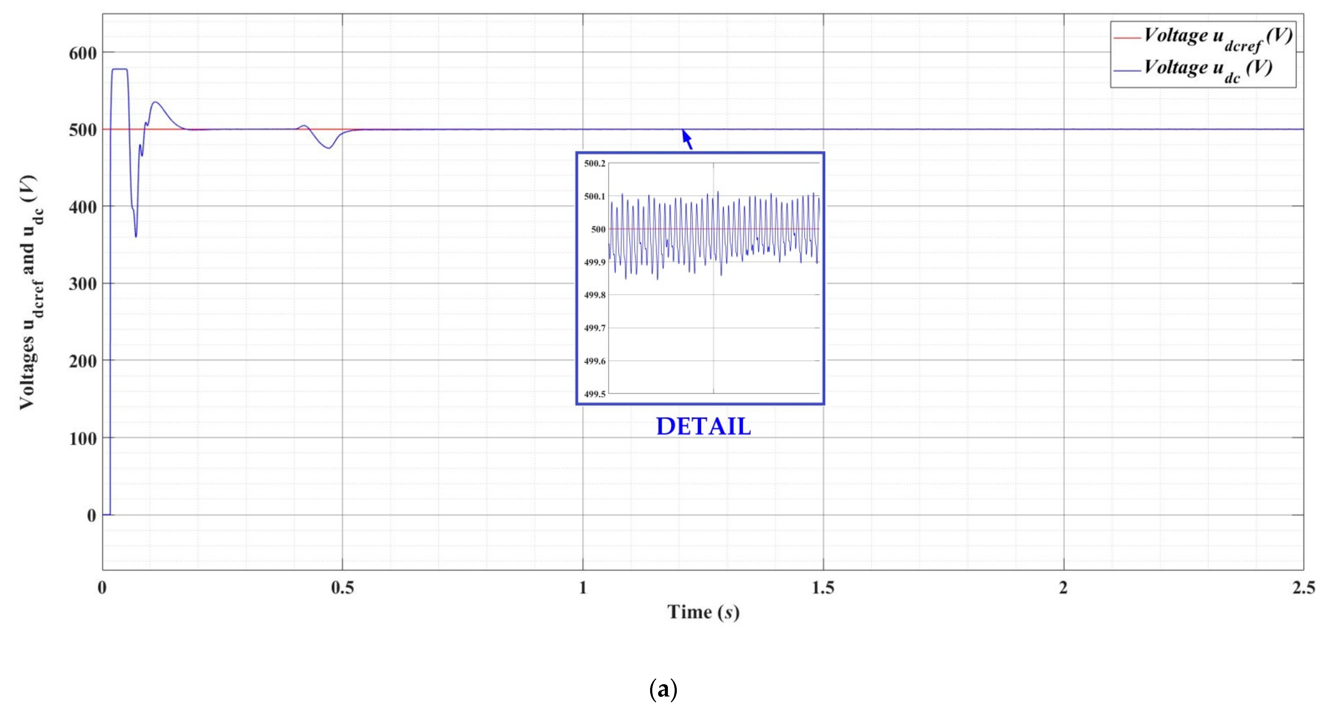
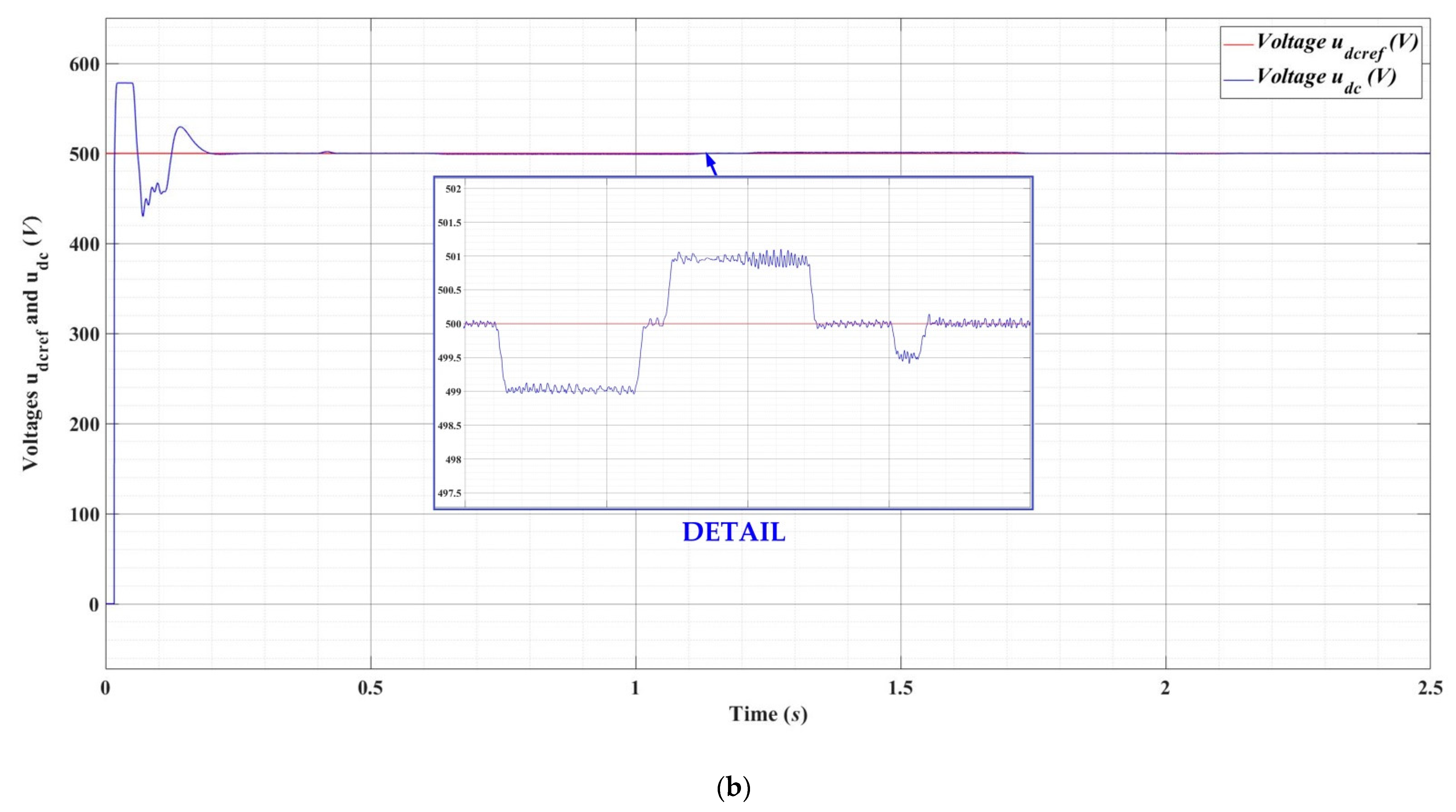
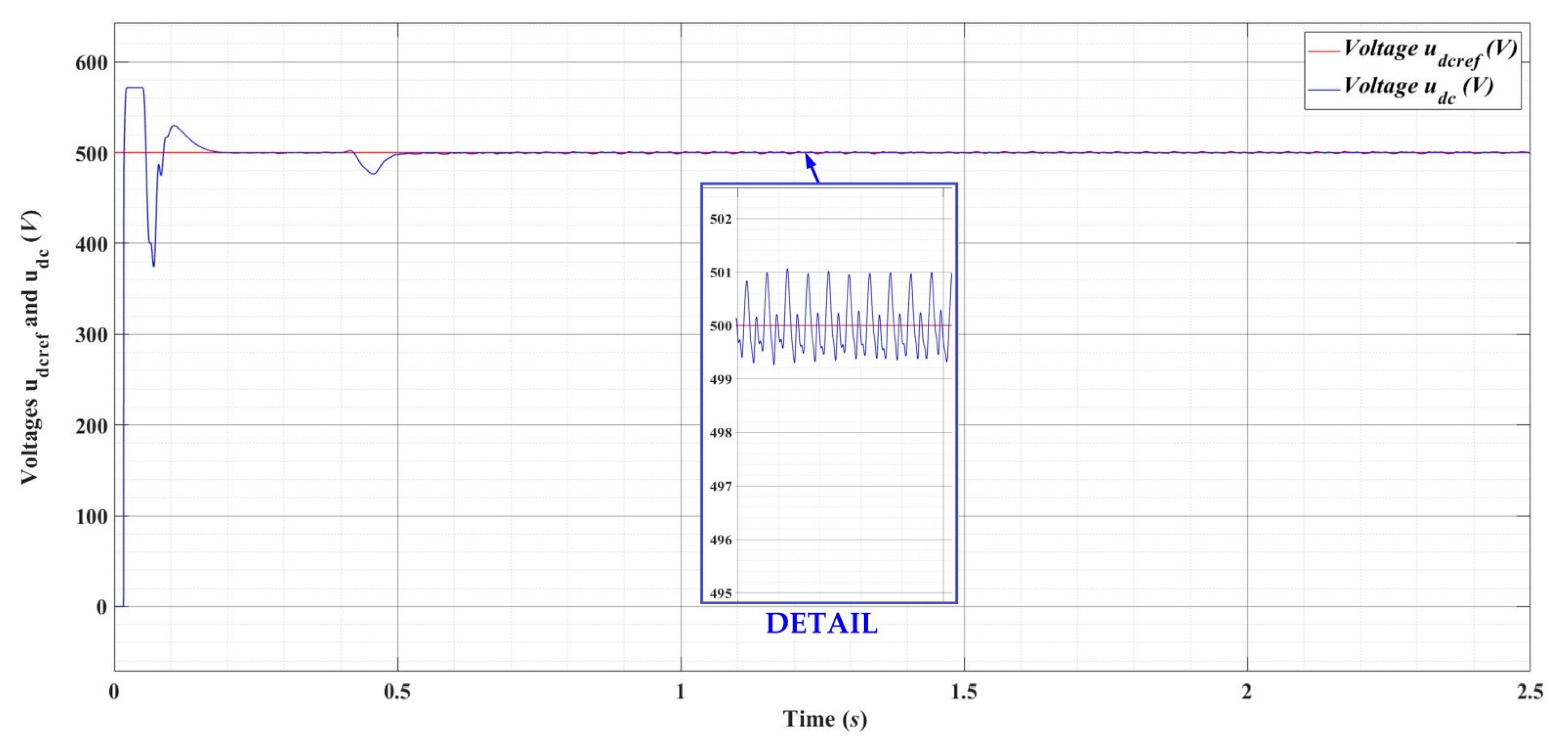
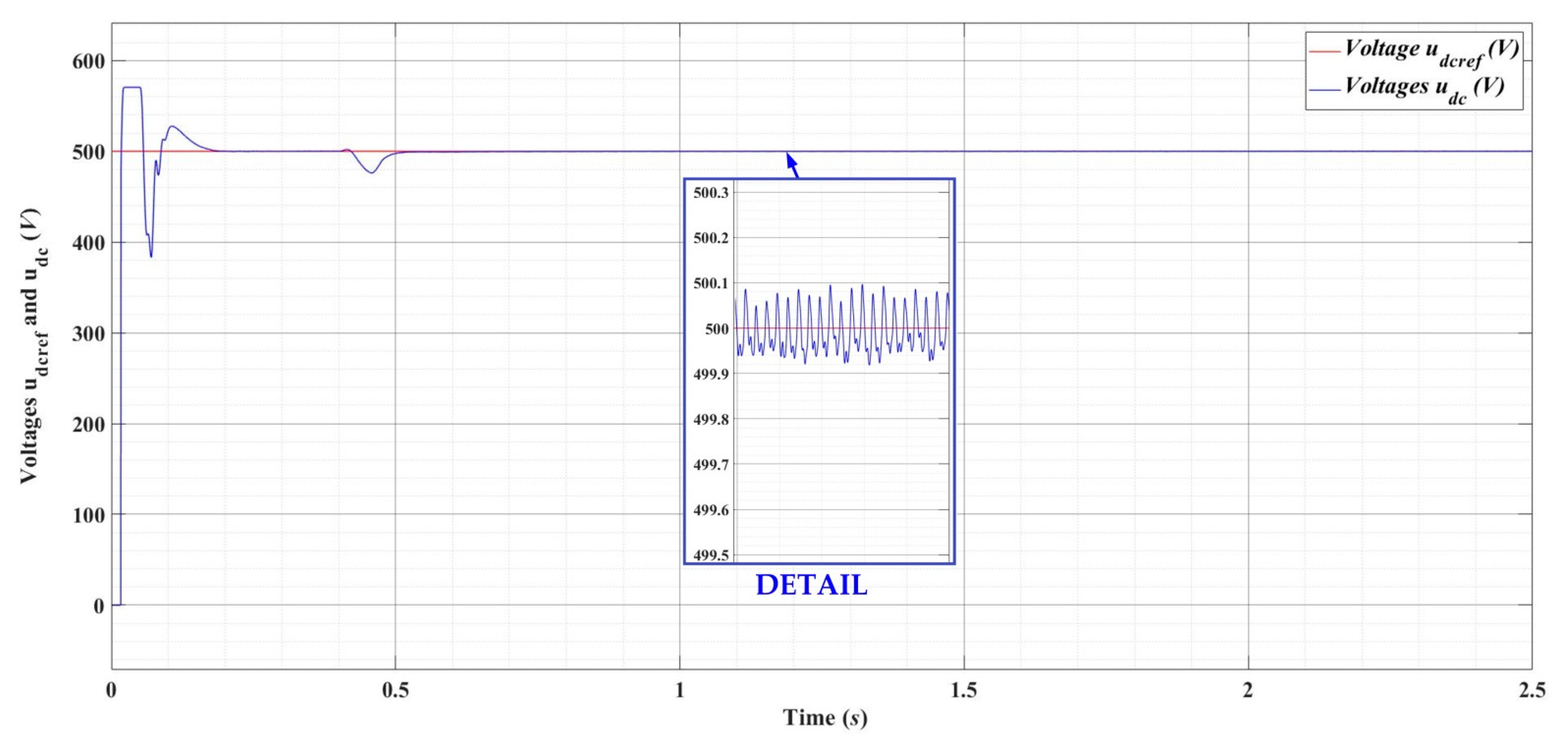
Figure 8a shows the response of the FO-SMC type control system for the control of the DC voltage u_dc combined with the FO-synergetic type control system for the control of currents i_d and i_q (FO-SMC/FO-SYN controllers), if the DC voltage reference u_dcref = 500 V, and Figure 8b shows the response of the control system where the controllers used for both the control of the DC voltage u_dc and for the control of currents i_d and i_q are of the PI type. After the validation of the control system start-up (after 50 ms), the MPPT algorithm start-up occurs (after 100 ms), and the end of the transitory regime (after 250 ms) is noted. In steady state, a steady-state error of 0.1 V, i.e., 0.02%, is noted for the FO-SMC/FO-SYN controllers, while the steady-state error for the PI controller is of 1 V, i.e., 0.2%. If the load is varied by a 30% increase or decrease, reaching 13 or 7 kvar, respectively, the superiority of the control of the grid-connected PV system based on FO-SMC/FO-SYN controllers is noted in Figure 9 and Figure 10.

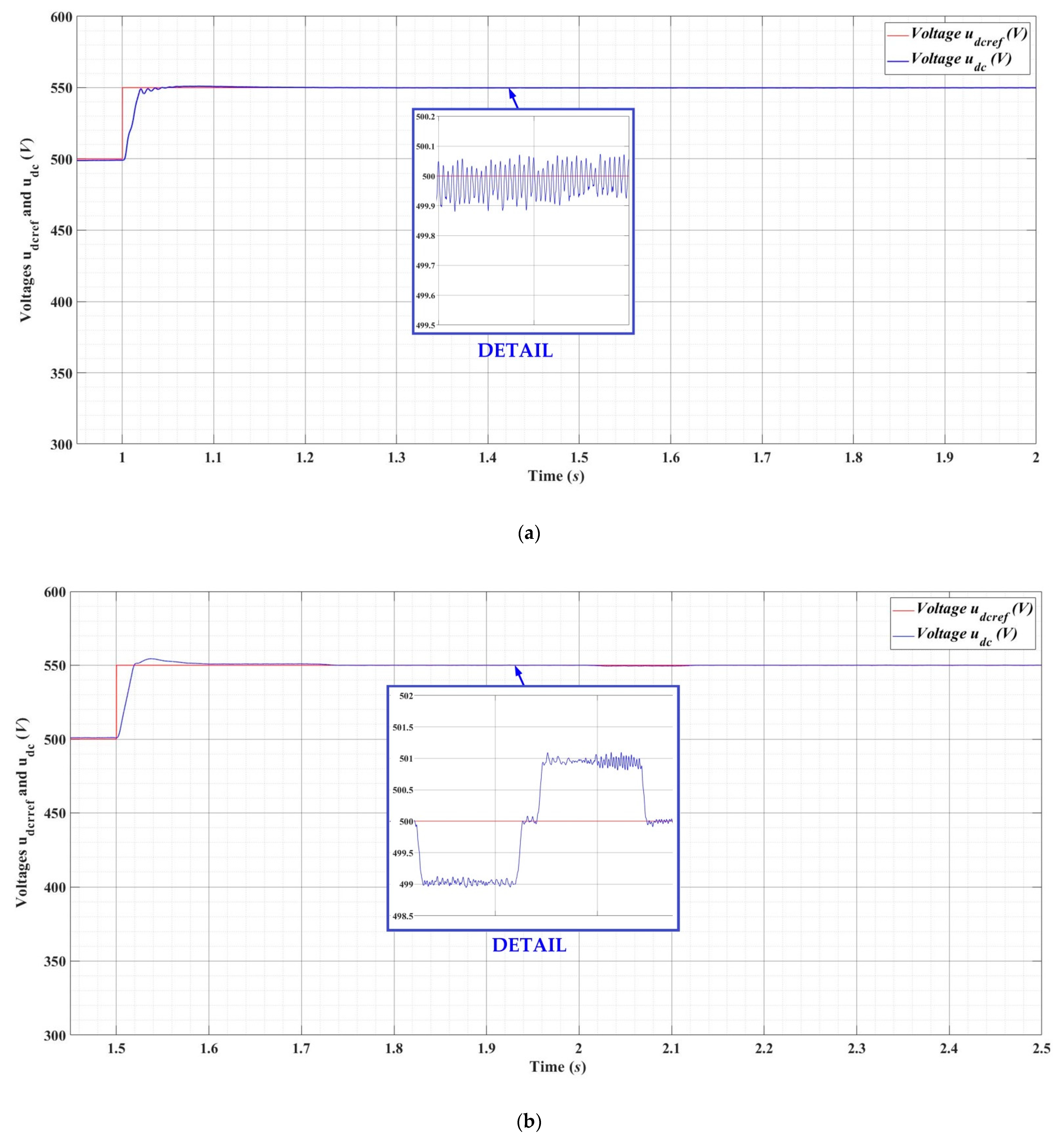
Regarding the dynamic regime, Figure 11 shows the response of the control of the grid-connected PV system based on FO-SMC/FO-SYN controllers as compared to PI controllers, where at time t = 1 s, the reference signal u_dcref undergoes a step variation at 550 V.

The parameters of the PI controller for u_dc control are K_p = 7 and K_i = 800 and the parameters of the PI controller for i_d and i_q currents are K_p = 0.3 and K_i = 20 [15].

The parameters of the FO-SMC/FO-SYN controllers (presented in Section 3) are; c₁ = 100; c₂ = 1; c₃ = 1; k = 180; ε = 110; C₂ = 6000e-06; T₁ = 0.01; T₂ = 0.01; K_p = 100; K_d = 0.2; L₃ = 2.5000e-04; R₃ = 0.0019; ω = 2·π·60.

It is noted that the performances in the dynamic regime, as well as those in the stationary regime, are superior in the case of using FO-SMC/FO-SYN controllers, and in Figure 11, an override of 0.2% (1 V) and a response time of 20 ms are noted, compared to an override of 1% (5 V) and a response time of 50 ms in the case of PI controllers.

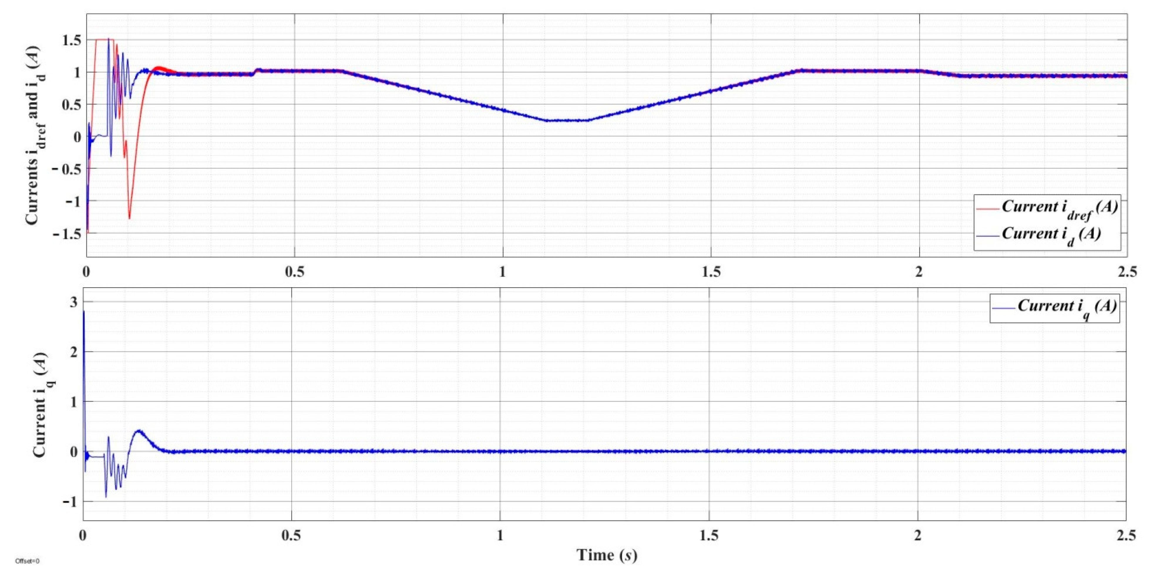
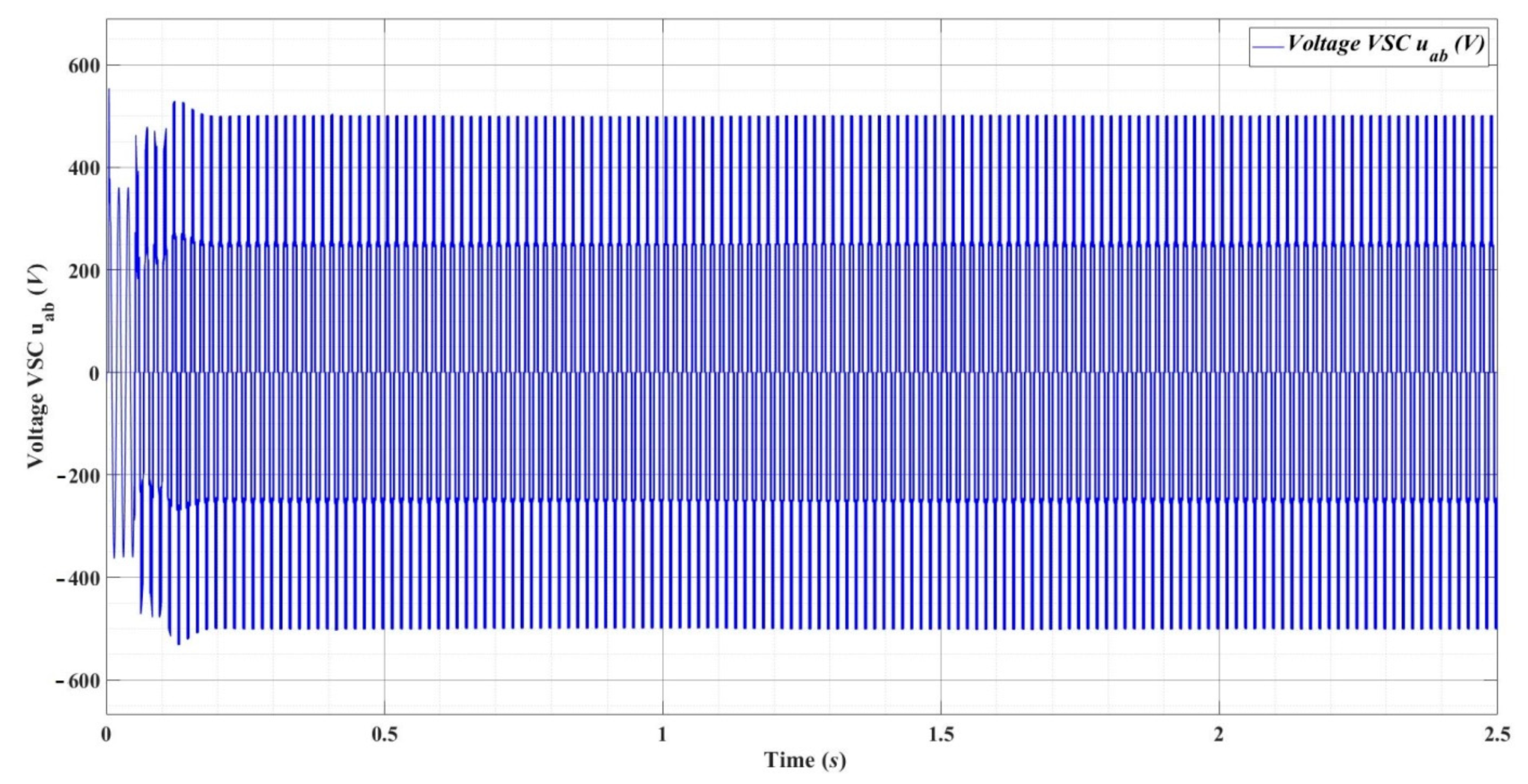
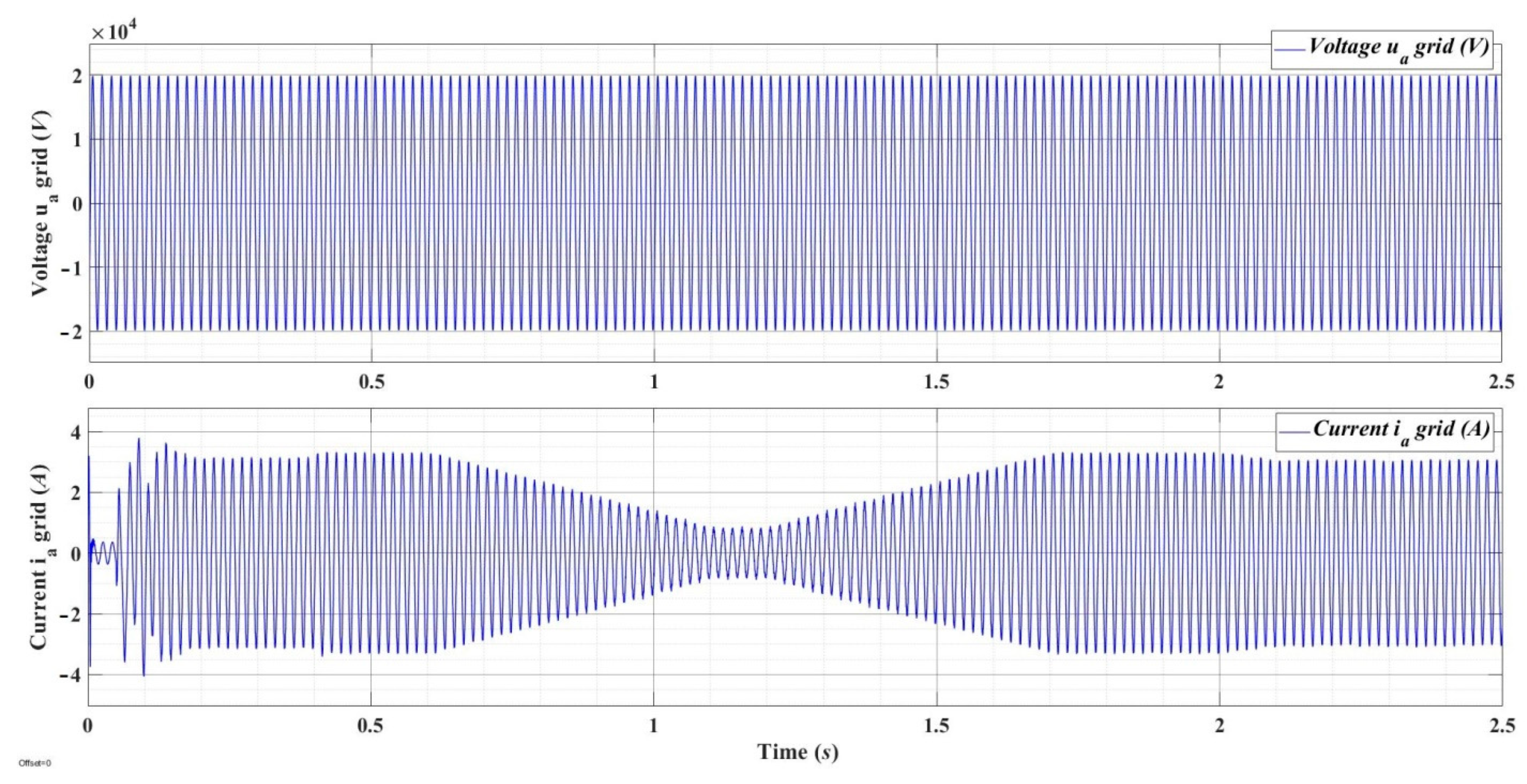
Figure 12, Figure 13, Figure 14, Figure 15 and Figure 16 show a series of waveform graphs regarding the time evolution of the main inputs of interest in the control of the grid-connected PV system. Thus, Figure 12 shows the time evolution of i_d and i_q currents, where it is noted that i_d follows the i_dref reference provided by the FO-SMC controller, while i_q follows the set reference i_qref = 0. Figure 13 shows the evolution of the average power and voltage of the PV array, P_mean and U_mean. Further, with regard to the DC-DC converter, Figure 13 presents the time evolution of the duty cycle signal provided by the MPPT algorithm, and with regard to the DC-AC converter, it presents the time evolution of the modulation index, a signal which is supplied by the control system of the VSC controller, which supplies control pulses. Figure 14 shows the evolution over time of the output voltage between two phases of the DC-AC converter. Figure 15 shows the time evolution of the voltage and current on a phase of the transformer for the connection to the main grid.

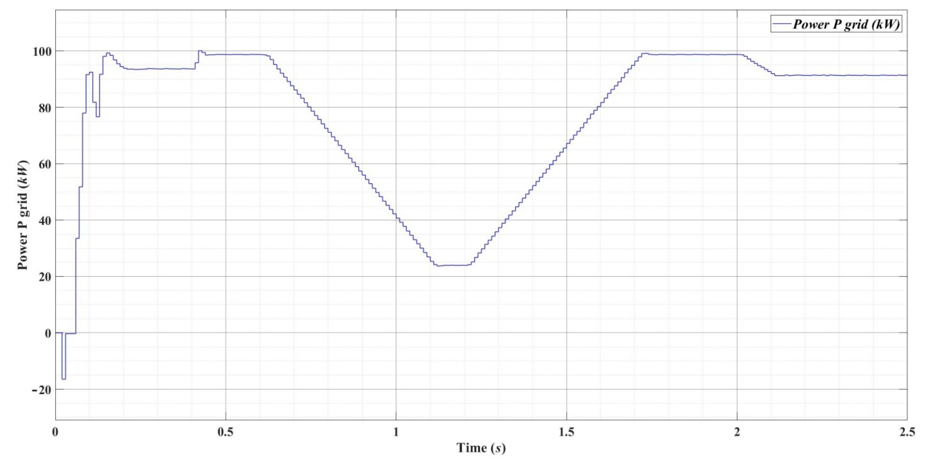
Moreover, Figure 16 shows the time evolution of the active power which flows between the analyzed system and the main grid.

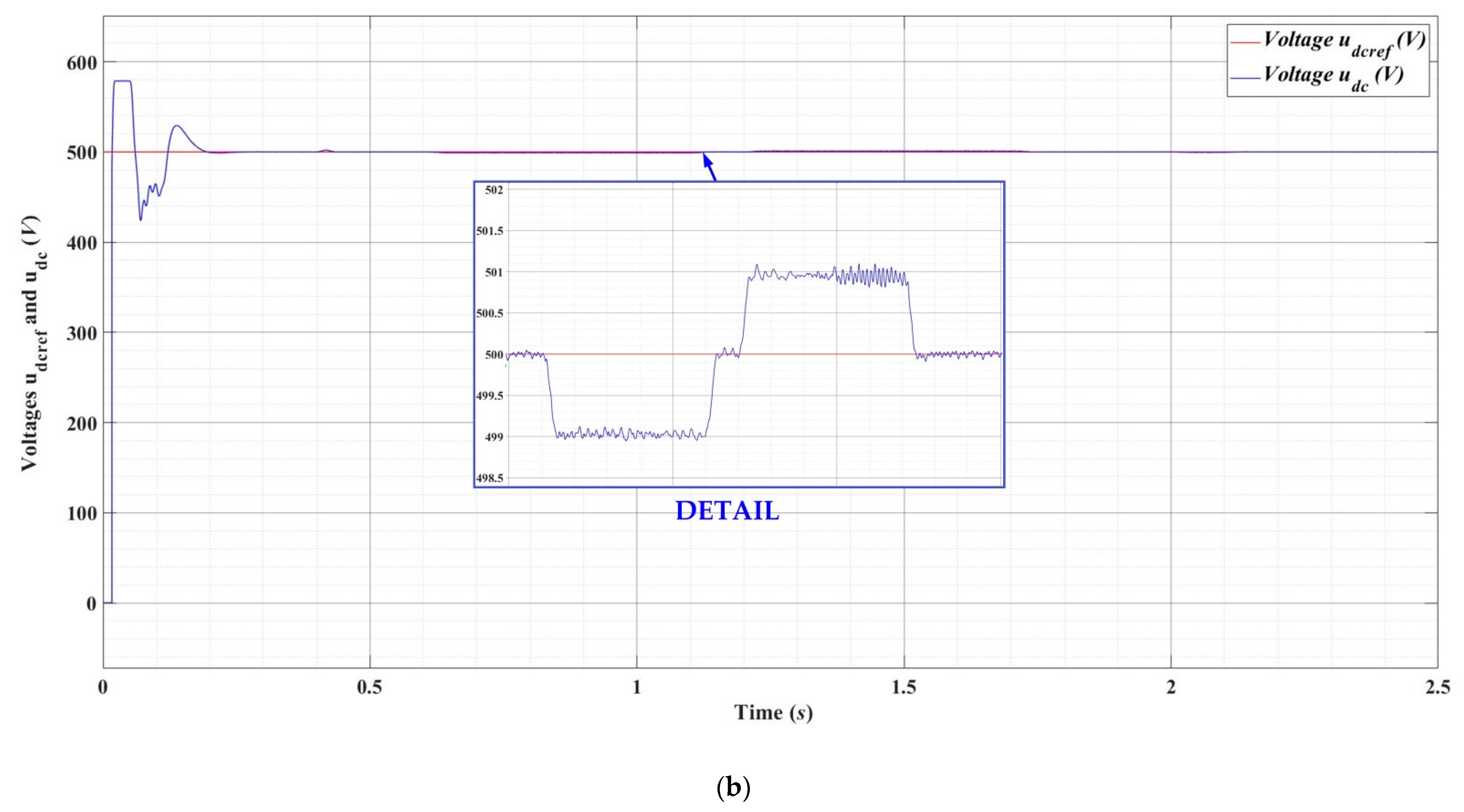
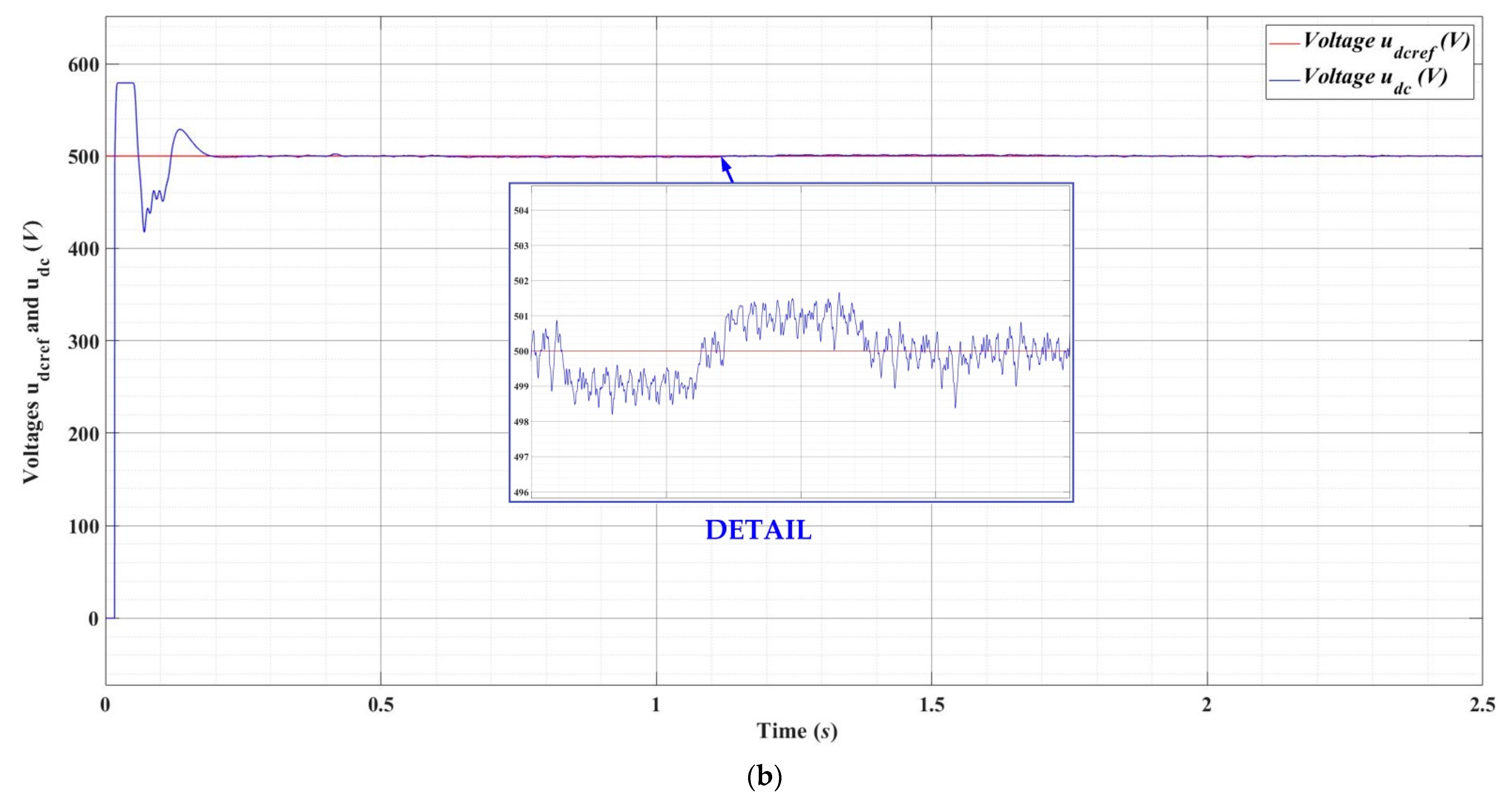
The control of the grid-connected PV system implemented in [15] is also discussed in [26], in which the control system of u_dc voltage is of the SMC type, the control systems of currents i_d and i_q are of the classic PI type, and the time evolution of the irradiance and temperature signals is presented in Figure 17. For the FO-SMC/FO-SYN controllers proposed in this article, Figure 18, Figure 19 and Figure 20 show the time evolution of the voltage u_dc in the DC intermediate circuit, if the reference voltage u_dcref is of 500 V. Superior performances are also noted in this case, both for the nominal load of 10 kvar and for its variations to 13 and 7 kvar. It is noted that the steady-state error is maintained at 0.1 V (0.02%).

Due to the fact that the basic model in Matlab/Simulink is complex and has all the aspects regarding the transformation chain from the PV array to the main grid connection and considering that it is used for comparison in other papers [15,26,27,31], this model can be considered as a benchmark for the control of the grid-connected PV system. Thus, the superior performance obtained by using the FO-SMC/FO-SYN controllers proposed in this article can be considered as a validation of the proposed control system.

5. Conclusions

This article presents the control of a grid-connected PV system using FO-SMC and FO-synergetic controllers. The mathematical model of a PV system connected to the main grid is presented together with the chain of intermediate elements: the DC-DC boost converter, the DC intermediate circuit, the DC-AC converter, the filtering block, and the transformer for the connection to the main grid, together with their control systems. The robustness and superior performance of an SMC-type controller for the control of u_dc voltage in the DC intermediate circuit are combined with the advantages provided by the flexibility of using synergetic control for the control of currents i_d and i_q. In addition, these control techniques are suitable for the control of nonlinear systems, and it is not necessary to linearize the controlled system around a static operating point; thus, the control system achieved is robust to parametric variations and provides the required static and dynamic performance. Further, by approaching the synthesis of these controllers using the fractional calculus for integration and differentiation operators, this article proposes a control system based on FO-SMC/FO-SYN controllers. The validation of the synthesis of the proposed control system is achieved by comparing it with a benchmark for the control of a grid-connected PV system implemented in Matlab/Simulink.

References

- Tricarico, T.; Gontijo, G.; Neves, M.; Soares, M.; Aredes, M.; Guerrero, J.M. Control Design, Stability Analysis and Experimental Validation of New Application of an Interleaved Converter Operating as a Power Interface in Hybrid Microgrids. Energies 2019, 12, 437. [Google Scholar] [CrossRef] [Green Version]
- Petersen, L.; Iov, F.; Tarnowski, G.C. A Model-Based Design Approach for Stability Assessment, Control Tuning and Verification in Off-Grid Hybrid Power Plants. Energies 2020, 13, 49. [Google Scholar] [CrossRef] [Green Version]
- Veerashekar, K.; Askan, H.; Luther, M. Qualitative and Quantitative Transient Stability Assessment of Stand-Alone Hybrid Microgrids in a Cluster Environment. Energies 2020, 13, 1286. [Google Scholar] [CrossRef] [Green Version]
- Zhao, F.; Yuan, J.; Wang, N.; Zhang, Z.; Wen, H. Secure Load Frequency Control of Smart Grids under Deception Attack: A Piecewise Delay Approach. Energies 2019, 12, 2266. [Google Scholar] [CrossRef] [Green Version]
- Montoya, O.D.; Gil-González, W.; Rivas-Trujillo, E. Optimal Location-Reallocation of Battery Energy Storage Systems in DC Microgrids. Energies 2020, 13, 2289. [Google Scholar] [CrossRef]
- Alshehri, J.; Khalid, M.; Alzahrani, A. An Intelligent Battery Energy Storage-Based Controller for Power Quality Improvement in Microgrids. Energies 2019, 12, 2112. [Google Scholar] [CrossRef] [Green Version]
- Estévez-Bén, A.A.; Alvarez-Diazcomas, A.; Rodríguez-Reséndiz, J. Transformerless Multilevel Voltage-Source Inverter Topology Comparative Study for PV Systems. Energies 2020, 13, 3261. [Google Scholar] [CrossRef]
- Yan, X.; Cui, Y.; Cui, S. Control Method of Parallel Inverters with Self-Synchronizing Characteristics in Distributed Microgrid. Energies 2019, 12, 3871. [Google Scholar] [CrossRef] [Green Version]
- Coppola, M.; Guerriero, P.; Dannier, A.; Daliento, S.; Lauria, D.; Del Pizzo, A. Control of a Fault-Tolerant Photovoltaic Energy Converter in Island Operation. Energies 2020, 13, 3201. [Google Scholar] [CrossRef]
- Khan, K.; Kamal, A.; Basit, A.; Ahmad, T.; Ali, H.; Ali, A. Economic Load Dispatch of a Grid-Tied DC Microgrid Using the Interior Search Algorithm. Energies 2019, 12, 634. [Google Scholar] [CrossRef] [Green Version]
- Cook, M.D.; Trinklein, E.H.; Parker, G.G.; Robinett, R.D., III; Weaver, W.W. Optimal and Decentralized Control Strategies for Inverter-Based AC Microgrids. Energies 2019, 12, 3529. [Google Scholar] [CrossRef] [Green Version]
- Oviedo Cepeda, J.C.; Osma-Pinto, G.; Roche, R.; Duarte, C.; Solano, J.; Hissel, D. Design of a Methodology to Evaluate the Impact of Demand-Side Management in the Planning of Isolated/Islanded Microgrids. Energies 2020, 13, 3459. [Google Scholar] [CrossRef]
- Stadler, M.; Pecenak, Z.; Mathiesen, P.; Fahy, K.; Kleissl, J. Performance Comparison between Two Established Microgrid Planning MILP Methodologies Tested On 13 Microgrid Projects. Energies 2020, 13, 4460. [Google Scholar] [CrossRef]
- Artale, G.; Caravello, G.; Cataliotti, A.; Cosentino, V.; Di Cara, D.; Guaiana, S.; Nguyen Quang, N.; Palmeri, M.; Panzavecchia, N.; Tinè, G. A Virtual Tool for Load Flow Analysis in a Micro-Grid. Energies 2020, 13, 3173. [Google Scholar] [CrossRef]
- MathWorks—Detailed Model of a 100-kW Grid-Connected PV Array. Available online: https://nl.mathworks.com/help/physmod/sps/ug/detailed-model-of-a-100-kw-grid-connected-pv-array.html;jsessionid=29903e2e045151ffb3e27a4920e1 (accessed on 4 November 2020).
- Hong, W.; Tao, G. An Adaptive Control Scheme for Three-phase Grid-Connected Inverters in Photovoltaic Power Generation Systems. In Proceedings of the Annual American Control Conference (ACC), Milwaukee, WI, USA, 27–29 June 2018; pp. 899–904. [Google Scholar]
- Naderi, M.; Khayat, Y.; Bevrani, H. Robust Multivariable Microgrid Control Synthesis and Analysis. Energy Procedia 2016, 100, 375–387. [Google Scholar] [CrossRef] [Green Version]
- Hua, H.; Qin, Y.; Xu, H.; Hao, C.; Cao, J. Robust Control Method for DC Microgrids and Energy Routers to Improve Voltage Stability in Energy Internet. Energies 2019, 12, 1622. [Google Scholar] [CrossRef] [Green Version]
- Villalón, A.; Rivera, M.; Salgueiro, Y.; Muñoz, J.; Dragičević, T.; Blaabjerg, F. Predictive Control for Microgrid Applications: A Review Study. Energies 2020, 13, 2454. [Google Scholar] [CrossRef]
- Zeb, K.; Islam, S.U.; Din, W.U.; Khan, I.; Ishfaq, M.; Busarello, T.D.C.; Ahmad, I.; Kim, H.J. Design of Fuzzy-PI and Fuzzy-Sliding Mode Controllers for Single-Phase Two-Stages Grid-Connected Transformerless Photovoltaic Inverter. Electronics 2019, 8, 520. [Google Scholar] [CrossRef] [Green Version]
- Kamal, T.; Karabacak, M.; Perić, V.S.; Hassan, S.Z.; Fernández-Ramírez, L.M. Novel Improved Adaptive Neuro-Fuzzy Control of Inverter and Supervisory Energy Management System of a Microgrid. Energies 2020, 13, 4721. [Google Scholar] [CrossRef]
- Song, L.; Huang, L.; Long, B.; Li, F. A Genetic-Algorithm-Based DC Current Minimization Scheme for Transformless Grid-Connected Photovoltaic Inverters. Energies 2020, 13, 746. [Google Scholar] [CrossRef] [Green Version]
- Yoshida, Y.; Farzaneh, H. Optimal Design of a Stand-Alone Residential Hybrid Microgrid System for Enhancing Renewable Energy Deployment in Japan. Energies 2020, 13, 1737. [Google Scholar] [CrossRef] [Green Version]
- Younesi, A.; Shayeghi, H.; Siano, P. Assessing the Use of Reinforcement Learning for Integrated Voltage/Frequency Control in AC Microgrids. Energies 2020, 13, 1250. [Google Scholar] [CrossRef] [Green Version]
- Serra, F.M.; Fernández, L.M.; Montoya, O.D.; Gil-González, W.; Hernández, J.C. Nonlinear Voltage Control for Three-Phase DC-AC Converters in Hybrid Systems: An Application of the PI-PBC Method. Electronics 2020, 9, 847. [Google Scholar] [CrossRef]
- Wu, B.; Zhou, X.; Ma, Y. Bus Voltage Control of DC Distribution Network Based on Sliding Mode Active Disturbance Rejection Control Strategy. Energies 2020, 13, 1358. [Google Scholar] [CrossRef] [Green Version]
- Qian, J.; Li, K.; Wu, H.; Yang, J.; Li, X. Synergetic Control of Grid-Connected Photovoltaic Systems. Int. J. Photoenergy 2017, 2107, 1–11. [Google Scholar] [CrossRef]
- Tepljakov, A. Fractional-Order Calculus Based Identification and Control of Linear Dynamic Systems. Master’s Thesis, Department of Computer Control, Tallinn University of Technology, Tallinn, Estonia, 2011. [Google Scholar]
- Tepljakov, A.; Petlenkov, E.; Belikov, J. FOMCON: Fractional-order modeling and control toolbox for MATLAB. In Proceedings of the 18th International Conference Mixed Design of Integrated Circuits and Systems—MIXDES, Gliwice, Poland, 16–18 June 2011; pp. 684–689. [Google Scholar]
- Mehiri, A.; Bettayeb, M.; Hamid, A. Fractional Nonlinear Synergetic Control for Three Phase Inverter Tied to PV System. In Proceedings of the 8th International Conference on Modeling Simulation and Applied Optimization (ICMSAO), Manama, Bahrain, 15–17 April 2019; pp. 1–5. [Google Scholar]
- de Brito, M.A.G.; Sampaio, L.P.; Luigi, G.; e Melo, G.A.; Canesin, C.A. Comparative analysis of MPPT techniques for PV applications. In Proceedings of the International Conference on Clean Electrical Power (ICCEP), Ischia, Italy, 14–16 June 2011; pp. 99–104. [Google Scholar]
- Nicola, M.; Nicola, C.-I. Sensorless Fractional Order Control of PMSM Based on Synergetic and Sliding Mode Controllers. Electronics 2020, 9, 1494. [Google Scholar] [CrossRef]
Figure 1.
Block diagram of the main circuit diagram of the grid-connected PV system.
Figure 2.
Block diagram of fractional-order sliding mode control (FO-SMC) and FO-synergetic control of the grid-connected PV system.
Figure 3.
General scheme for cascade control of the grid-connected PV system.
Figure 4.
Matlab/Simulink implementation block diagram for control of the grid-connected PV system using FO-SMC and FO-synergetic controllers.
Figure 5.
Matlab/Simulink implementation block diagram for the FO-SMC controller.
Figure 6.
Matlab/Simulink implementation block diagram for FO-synergetic controllers.
Figure 7.
Time evolution of the irradiance and temperature signals type 1.
Figure 8.
Time evolution of the udc for the irradiance and temperature signals type 1, at 10 kvar load: (a) FO-SMC/FO-SYN controllers; (b) classical PI controllers.
Figure 9.
Time evolution of the udc for the irradiance and temperature signals type 1, at 13 kvar load: (a) FO-SMC/FO-SYN controllers; (b) classical PI controllers.
Figure 10.
Time evolution of the udc for the irradiance and temperature signals type 1, at 7 kvar load: (a) FO-SMC/FO-SYN controllers; (b) classical PI controllers.
Figure 11.
Time evolution of the udc for the irradiance and temperature signals type 1, at 10 kvar load for a step variation of udcref from 500 to 550 V: (a) FO-SMC/FO-SYN controllers; (b) classical PI controllers.
Figure 12.
Time evolution of the id and iq currents.
Figure 13.
Time evolutions of the power Pmean and voltage Umean of the PV, duty cycle of the DC-DC converter, and modulation index of the DC-AC converter.
Figure 14.
Time evolution of the voltage uab of the voltage source converter (VSC) controller.
Figure 15.
Time evolution of the voltage ua and current ia of the main grid.
Figure 16.
Time evolution of the power flow P between PV system and main grid.
Figure 17.
Time evolution of the irradiance and temperature signals type 2.
Figure 18.
Time evolution of the udc for the irradiance and temperature signals type 2, at 10 kvar load with FO-SMC/FO-SYN controllers.
Figure 19.
Time evolution of the udc for the irradiance and temperature signals type 2, at 13 kvar load with FO-SMC/FO-SYN controllers.
Figure 20.
Time evolution of the udc for the irradiance and temperature signals type 2, at 7 kvar load with FO-SMC/FO-SYN controllers.
Publisher’s Note: MDPI stays neutral with regard to jurisdictional claims in published maps and institutional affiliations. |
© 2021 by the authors. Licensee MDPI, Basel, Switzerland. This article is an open access article distributed under the terms and conditions of the Creative Commons Attribution (CC BY) license (http://creativecommons.org/licenses/by/4.0/).
Share and Cite
MDPI and ACS Style
Nicola, M.; Nicola, C.-I. Fractional-Order Control of Grid-Connected Photovoltaic System Based on Synergetic and Sliding Mode Controllers. Energies 2021, 14, 510. https://0-doi-org.brum.beds.ac.uk/10.3390/en14020510
AMA Style
Nicola M, Nicola C-I. Fractional-Order Control of Grid-Connected Photovoltaic System Based on Synergetic and Sliding Mode Controllers. Energies. 2021; 14(2):510. https://0-doi-org.brum.beds.ac.uk/10.3390/en14020510
Chicago/Turabian StyleNicola, Marcel, and Claudiu-Ionel Nicola. 2021. "Fractional-Order Control of Grid-Connected Photovoltaic System Based on Synergetic and Sliding Mode Controllers" Energies 14, no. 2: 510. https://0-doi-org.brum.beds.ac.uk/10.3390/en14020510
Note that from the first issue of 2016, this journal uses article numbers instead of page numbers. See further details here.