Energy Flexibility as Additional Energy Source in Multi-Energy Systems with District Cooling


1
Dipartimento di Ingegneria Industriale e Scienze Matematiche, Università Politecnica delle Marche, Via Brecce Bianche 12, 60131 Ancona, Italy
2
Consiglio Nazionale delle Ricerche, Istituto per le Tecnologie della Costruzione, Viale Lombardia 49, San Giuliano Milanese, 20098 Milan, Italy
3
Department of Mechanical Engineering, KU Leuven, B-3000 Leuven, Belgium
*
Author to whom correspondence should be addressed.
Energies 2021, 14(2), 519; https://0-doi-org.brum.beds.ac.uk/10.3390/en14020519
Submission received: 17 December 2020
/
Revised: 8 January 2021
/
Accepted: 12 January 2021
/
Published: 19 January 2021
(This article belongs to the Special Issue Refrigeration, Air Conditioning and Heat Pumps: Energy and Environmental Issues II)
Abstract
:The integration of multi-energy systems to meet the energy demand of buildings represents one of the most promising solutions for improving the energy performance of the sector. The energy flexibility provided by the building is paramount to allowing optimal management of the different available resources. The objective of this work is to highlight the effectiveness of exploiting building energy flexibility provided by thermostatically controlled loads (TCLs) in order to manage multi-energy systems (MES) through model predictive control (MPC), such that energy flexibility can be regarded as an additional energy source in MESs. Considering the growing demand for space cooling, a case study in which the MPC is used to satisfy the cooling demand of a reference building is tested. The multi-energy sources include electricity from the power grid and photovoltaic modules (both of which are used to feed a variable-load heat pump), and a district cooling network. To evaluate the varying contributions of energy flexibility in resource management, different objective functions—namely, the minimization of the withdrawal of energy from the grid, of the total energy cost and of the total primary energy consumption—are tested in the MPC. The results highlight that using energy flexibility as an additional energy source makes it possible to achieve improvements in the energy performance of an MES building based on the objective function implemented, i.e., a reduction of 53% for the use of electricity taken from the grid, a 43% cost reduction, and a 17% primary energy reduction. This paper also reflects on the impact that the individual optimization of a building with a multi-energy system could have on other users sharing the same energy sources.
1. Introduction
In recent years, programs aimed at increasing the efficiency and sustainability of the building sector have entered into force all over the world. For instance, the Energy Performance of Buildings Directive (EPBD) [1] in the European Union (EU) requires Member States to reduce the energy demand of their entire building stock by 80% before 2050 by transitioning to nearly zero energy buildings (NZEBs). In addition to encouraging strategies for reducing the buildings’ energy requirements for heating and cooling, it also suggests the consideration of optimal combinations of available energy sources (e.g., renewable energy sources (RESs), district heating (DH) and district cooling (DC)) when planning, designing, building and renovating industrial or residential areas [1]. Conventionally, in fact, the different building energy requirements have been met by individual energy carriers that do not interact with each other. However, the exploitation of their optimal combination could increase both the efficiency and the flexibility of local energy systems [2].
When a number of different energy sources are integrated into a building, this is referred to as a hybrid or multi-energy system (MES). An MES is where electricity, heating, fuels, and other types of energy vectors interact optimally with each other at various levels [3]. Focusing on residential buildings, natural gas and electricity can be energy sources for various generators, including boilers, electric heat pumps (HPs), chillers and combined heat and power (CHP) systems, which can then be used to produce electricity, heating and cooling [3]. Furthermore, MESs can integrate RESs and use energy sources recovered from optimized system management (e.g., harvesting energy from natural gas distribution networks [4]). Furthermore, the interaction of buildings at the district level (e.g., heating or cooling energy in DH or DC) can be exploited, and building loads can be easily shifted thanks to the different energy storage systems that can be integrated in MESs [5]. In this way, energy flexibility can be considered as an energy source in its own right.
Several configurations of multi-energy systems applied to buildings have been analyzed in the literature with the aim of showing their effectiveness in terms of efficiency and sustainability. For instance, Aste et al. [6] introduced a fully renewable urban district in which a low-temperature and small-sized wood biomass district thermal plant was integrated with groundwater heat pumps and solar photovoltaic (PV) systems. Energy simulation demonstrated that controlled exploitation of multiple energy sources in a district heating system allowed for greater self-consumption of renewable sources, with a low request for grid electricity. Liu et al. [7] determined a 40% reduction in CO2 emissions when a hybrid HVAC (Heating, Ventilation and Air Conditioning) system, consisting of a CHP plant and a liquid-desiccant system, was used to match the power and thermal demand of a demonstration building in Beijing, China.
Other papers have focused on the identification of optimal operating strategies for specific MES systems in order to achieve specific energy objectives. For instance, Ren et al. [8] assessed a multi-objective optimization model in order to determine the optimal strategy for a distributed energy source system. The case study comprised an energy system installed in an eco-campus in Japan, and included several different sources (photovoltaic, fuel cell, and gas engine). The minimization of two objective functions, i.e., energy cost and CO2 emissions, was achieved by means of a compromise programming method. The results showed that the increase in the degree of satisfaction of economic objectives led to increased CO2 emissions. To take into account the complex relationship among energy systems in MESs, Ruusu et al. [9] described a new energy management system for a variety of energy flexibility conversion technologies and storage options in buildings by means of a nonlinear optimization-based model predictive control (MPC) method.
District heating and cooling systems are relevant resources in efficient multi-energy systems, and their integration with respect to building energy demand has received a great deal of attention. For instance, Aoun et al. [10] presented a MILP-based (mixed-integer linear programming) model predictive control in order to satisfy thermal demand in buildings connected to a district heating system. In particular, they investigated the exploitation of the thermal mass embedded in the building envelope to optimally schedule space heating loads on the basis of weather conditions and energy cost variations. Luc et al. [11] also exploited the thermal mass of the buildings for the purpose of heat storage and evaluated the flexible operation potential of a small district with buildings connected to a district heating network. Introducing different load shifting scenarios based on thermal demand data and heat production cost in the Greater Copenhagen district heating system, they obtained a potential load shifting of between 41% and 51% in all of the considered scenarios. Even Foteinaki et al. [12] investigated the potential for the flexible operation of low-energy residential buildings in district heating systems. They demonstrated that, using the thermal mass of the building as a storage medium, the pre-heating strategy was highly effective for load shifting and peak load reduction (energy use was reduced in all scenarios by between 40% and 87%). An analysis of the literature confirms the relevant role that the flexibility provided by thermostatically controlled loads can have in the optimal management of MESs. Furthermore, among the other resources of an MES, district cooling systems are very promising systems for increasing the energy efficiency of the cooling sector [13], but there are still few works considering their integration with building loads and their optimization, with much more emphasis having been given to district heating systems [14]. Cooling loads and thermal comfort in summer have their own specific characterizations that are distinct from the winter season; therefore, an ad hoc analysis is needed. For example, Zabala et al. [15] presented the case of a district cooling with absorption machines, whose production was controlled through a model predictive control. In the present paper, the integration of district cooling systems with building energy demand is also investigated, but in contrast with previous works, the district cooling system is considered to be supplied using waste energy. This scenario is derived from the exploitation of cooling power from a particular energy recovery process that has already been presented in a previous work [16], where the evaporation of liquefied natural gas in a fuel station was able to provide cold energy to a small residential district cooling network. Therefore, the cooling power provided to the DC follows a given load curve and cannot be optimized, as in the literature works described above. Moreover, the objective of this work is focused at the building level, where the available cold energy is deployed at best in combination with the other energy sources composing the multi-energy system. The analysis aims to highlight the importance of the activation of building energy flexibility provided by thermostatically controlled loads (TCL), e.g., air conditioners and space cooling/heating systems. Such flexible energy loads are assumed in this analysis to be additional virtual energy resources in the optimal management of a building multi-energy system that also integrates a district cooling network.
When an MES is integrated into a building, an advanced control method is necessary to optimize the operational energy performance in a timely fashion. Thus, an MPC is considered for the analyzed case. Indeed, MPCs represent one of the most explored paradigms in the academic literature for realizing intelligent energy management in buildings [17], due to its capability of combining the principles of feedback control and numerical optimization [18]. The potential of such control to provide demand-side flexibility in buildings with multi-carrier energy systems has been discussed by Zong et al. [19]. They highlight that an MPC-based BEMS (Building Energy Management System) controller is an efficient and feasible approach for managing the portfolio of energy usage in buildings. An MPC uses a dynamic model to predict the system response in order to select the best sequence of control actions, taking into account both predictions of future disturbances and system constraints [20]. For short-term predictions, three categories of building energy models are available: white box, grey box and black box [21]. There are several contributions in the literature regarding the performance evaluation of the different building modeling approaches to be used in an MPC. Among others, Mugnini et al. [22] summarized the advantages and disadvantages of a data-driven model based on an artificial neural network (ANN) and a physical-based model based on a thermal network of resistances and capacitances to predict the building thermal demand in an operative MPC designed to minimize the total cost by using TLC flexibility. In a simplified case study, they highlighted the improved performance of the physical-based model in the exploitation of the energy flexibility derived from thermostatically controlled loads.
This paper presents, through the analysis of a case study, the manner in which the energy flexibility of TCL can be exploited to optimally manage a multi-energy system including district cooling. The manuscript is structured as follows: in Section 2, the generalized methodology for implementing an MPC in order to integrate different energy sources (including a district cooling) in an MES in a building is presented. Section 3 describes the case study, and in Section 4 the optimal control is applied to the case study. The results for the different objective functions are discussed in Section 5, while Section 6 provides the main conclusions of the study.
2. Methodology
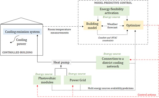
In this paper, a multi-energy system in a building is introduced as a case study. The concept of the application is represented in Figure 1: different energy sources (including flexibility from TCLs) are managed in real time, on the basis of their availability, by the controller in order to meet the building energy demand according to the minimization of a specific objective function (OF).
The mathematical problem is formulated in generalized terms and its effectiveness is tested in a case study. The evaluation of the optimal control of the MES is realized from two points of view. First, its operation in terms of seasonal energy performance is compared to the case with a traditional rule-based control. Second, the control robustness is evaluated by analyzing different interactions of the energy sources when different objective functions are pursued and control setting parameters (e.g., prediction horizon) are varied. Moreover, a focus on the impact of an optimized user on other buildings sharing the same energy sources (e.g., DC) is provided.
The case study consists of a single residential building whose cooling energy demand can be satisfied with different energy sources: the connection to a DC network and a variable-load air-to-water electrical heat pump (HP) that can be fed with either electricity produced by photovoltaic (PV) modules or supplied by the electricity from the grid. Additionally, a certain degree of energy flexibility is provided by a wider variation of the indoor air temperature setpoint of the thermostat. Variation of the cooling demand according to the setpoint can be exploited by the control as an additional virtual energy source.
Three different objective functions are tested in the optimal control; these are concerned with the minimization of: (i) the electricity taken from the grid, (ii) the overall energy costs, and (iii) the total primary energy consumption. The aim is to highlight how the specific objective function affects the exploitation of each energy source by the controller, demonstrating the importance of the activation of the energy flexibility in such advanced control of an MES.
In this section, a generalized MPC formulation is presented for exploiting an MES including district cooling in buildings. An MPC can be defined as a control that is able to update on-line the manipulated variables to satisfy multiple, changing performance criteria in the face of changing plant characteristics [23]. It is composed of two parts: the system response model and the optimizer. The system response model is used to predict the future states of the system over a certain period of time (prediction horizon, PH) in the presence of disturbances (uncontrolled inputs) and manipulated variables (controlled inputs). Starting from the system response prediction, the optimizer generates control actions to minimize a defined objective function within PH while respecting the system constraints [24]. The MPC follows a receding horizon logic [20]: at each time step (k), only the first control action is applied, and the next predictions and control actions are recalculated while shifting the prediction horizon forward.
When an MPC is used to control the HVAC of a building, the system model should be able to predict the building energy demand while respecting the comfort constraints. To do this, the MPC has to receive the predictions of the disturbances (such as the occupancy profile or weather conditions) as inputs throughout the PH. Then, if an MES is available, the control actions should lead to an optimal exploitation of each energy source according to the goal to be reached. Therefore, the optimizer should determine whether each source has to be used by the HVAC, while satisfying the energy requirements of the building. Thus, the predictions of energy source availability profiles must also be provided as inputs to the optimizer. In Figure 2, a scheme of the proposed MPC is presented, and the following subsections provide a detailed description of its formulation.
With this kind of control, a single building can satisfy its thermal requirements while optimizing its energy performance. However, when energy sources that involve the connection of different users (DC or DH) are used, there is no guarantee that, if all buildings are optimized independently from each other, the performance of the overall system will be optimized at the same time in the presence of constrained resources. In this sense, a preliminary analysis of the problem can be provided by evaluating, in terms of comfort violation, how users who are connected immediately after the controlled building will be affected by its operation. More details are provided in Section 4, where the generalized MPC formulation is applied to the case study. This section is divided into Section 2.1, where the building model is described in detail, and Section 2.2, which contains the formulation of the controller.
2.1. Building Model
To predict the thermal dynamics of the building, a lumped-parameter model based on the thermal electricity analogy is used. It relies on the heat balance method [25], which discretizes the building into thermal zones modeled using a network of nodes. The time evolution (system state) of each node is described by a temperature (T) and the capability of storing heat in the thermal mass is modeled with thermal capacitances (C) [26]. The heat fluxes between nodes are described by thermal resistances (R), and heat gains (Ġ) are directly applied to the thermal nodes. In this way, the building can be represented by an equivalent circuit of thermal resistances and capacitances (RC network).
Assuming a one-dimensional heat transfer, the system dynamics is described by a set of ordinary differential equations that can be represented as a classic linear state-space model (SSM):
where is the state-space vector, is the input vector, and represents the output vector. , , and are time-invariant real matrices depending on the parameters of the system (C and R).
Based on the number of thermal nodes with which the circuit is built, different order models can be obtained. However, to catch the short-term dynamics of the building, a second-order model, at least, is required [27]. To capture the dynamics of the internal air temperature, the air thermal capacity is distinguished from the total internal capacity, obtaining a third-order model (Figure 3).
The three thermal nodes ( and ) represent the temperatures of the envelope thermal mass, internal air, and internal thermal mass, respectively; consequently, and represent their thermal capacitances. Four thermal resistances are used: and . models the resistance to the heat transfer between the outdoor temperature () and due to windows and natural ventilation, while and are the thermal resistances between the building envelope thermal mass node () and and , respectively. is the thermal resistance between the internal thermal mass node () and . The heat fluxes applied to the thermal nodes and are: the contribution provided by the HVAC system () and the heating gains () divided by the internal () and the solar () components. Except for , which is applied entirely to , the other two fluxes are divided between the node by a factor f (fas and faq for the and contribution to , fis and fiq for the and contribution to ). Equations (3) and (4) represent the evolution of the system shown in SSM representation:
where represents the thermal conductance, calculated as the inverse of the thermal resistance ().
To identify the parameters of the model (, ,, , ), a white box approach is used. In this way, they are deduced from the knowledge of the building’s thermal and geometrical features. In particular, the stratigraphy of the envelope and the building materials should be known or hypothesized. With respect to the numerical value of the thermal capacitances, and represent the thermal masses which communicates with the external environment and internal environment, respectively. For each opaque structure (s) of the building, a thermal capacity () is calculated as follows:
where the index l represents a single material layer of the opaque structure s, refers to the inner layer (facing the internal zone), and is the thermal insulation layer position. and are the area and the heat capacity per area of the element l, respectively.
The thermal capacity relative to the indoor air () is defined as:
where , and are the volume, density and specific heat of the air, respectively.
Taking into account the thermal resistances, their numerical values are deduced on the basis of the thermal features of the building envelope. Equation (7) reports the expressions of :
where ACH represents the air change per hour, while is the product of the thermal transmittance and the area of the windows.
, and refer to the opaque structures (s) identified to evaluate and . Their numerical values can be calculated by adding the internal () and external thermal resistances for each surface s. In particular, as expressed in Equations (8) and (9) for a surface s, contains the contribution of all layers facing the internal zone that precede , while includes the remaining part of the external envelope (from to ).
where and are the internal and external surface thermal resistances, and are the thickness and the thermal conductivity of the layer l, while refers to the outer layer (facing the outdoor environment). The specific values of the resistances , and can be obtained by adding the contributions of the different surfaces (s) comprising the envelope and the internal thermal mass.
To validate the short-term predictive capability of the RC network, its operation is compared to the results of a building model with the same thermal and geometrical characteristics, developed in TRNSYS, which represents the “real” system in this analysis. The performance is assessed by evaluating the root mean square error, RMSE, which is defined as:
where N is the number of points considered, which corresponds to the model performance evaluation period according to the timestep k.
2.2. MPC Formulation for the MES
The application of a MPC to the HVAC of a building involves the real-time resolution of an optimization problem (OP), the classic control algorithm of which is based on a linear or quadratic objective function (OF), subject to equality or inequality constraints [28]. Then, the control acts to select the optimal sequence of manipulated variables over the PH by using predictions of building response (Section 2.1). Following the receding horizon logic, the optimal variables are transferred to the HVAC as control actions. To be effective, the MPC must be provided with the uncontrolled input profiles. Typically, they are represented by the system state disturbances, which, in the case of buildings, are the inputs required by the building model: the outdoor temperature (), and the heat gains ( and ), as shown in Equations (3) and (4). However, when the system operation involves the exploitation of an MES, the forecasts of energy source availability have to be included in the optimizer inputs (Figure 2). In this case, a distinction should be made between the energy sources that depend on the actual system state and those that do not. As described in Section 2.1, the system state is represented by the node temperatures (, and ), which are strongly linked to the thermal demand of the building (). Therefore, acts as a controlled input for the building model, and therefore as a continuous decision variable for the OP. In this context, the exploitation of an energy source can take place according to two different logics. When source availability is defined by a given profile (uncontrollable input), the system adapts its state to use a given source in the right measure. On the contrary, if the availability of the source is potentially limitless and its employment is strongly linked to the actual energy request of the building, this source has to be considered to be a manipulated variable in the OP. The latter category is represented by the energy sources taken from the grid (e.g., natural gas or electricity drawn from the grid). To formulate the control in general terms, this distinction among energy sources needs to be considered when defining the OP.
Let be the number of usable energy sources acting as uncontrolled inputs (index ) and the control timestep; is the availability profile for each at each timestep k, while is the energy source drawn from the grid (). Associating a penalty factor () to each energy source ( and ), the OP can be formulated in general terms (Equations (11) and (12)). By varying , the use of some sources rather than others can be penalized or encouraged according to the intended purpose of the OP (e.g., minimizing the total costs or the primary energy consumption).
In Equation (11), and are the conversion factors of and into thermal energy. Therefore, and represent the building thermal demand that can be covered by each e or drawn by the grid G. Since e refers to an uncontrollable input, its actual use is decided by a use factor ), acting as a continuous decision variable that can assume values between 0 and 1.
The OF defined in Equation (11) must be minimized while respecting some system constraints. Firstly, the internal comfort of the occupants has to be satisfied for each time k. This condition is represented by Equation (13), where and represent the permitted comfort band that can be exploited by the controller.
Equation (13) represents the link between the building model and the optimizer (Figure 2). If discretized, in fact, Equation (1) can be rewritten as:
In this way, the connection between and the decision variable can be expressed in a linear way. Furthermore, the optimization constraints related to the HVAC system must be defined. These concern the maximum capability () of the system involved (Equation (15)) and, if a withdrawal from the grid is envisaged, the constraint expressed by Equation (16) has to be added in order to avoid unacceptable solutions when the availability of the energy sources is too high (i.e., negative values of electricity drawn for the grid).
With this formulation, the OF, the decision variables, and the constraints are all linear functions. Therefore, the optimization problem can be treated as a typical linear programming (LP) problem, and the “dual-simplex” algorithm can be used in the controller. It is important to note that, to ensure the linearity of the OP, the presented formulation allows the involvement of a single energy source drawn from the grid. In fact, the latter is interpreted by the controller as a supplementary energy source to be used when the availability of other energy sources is not enough.
Once the optimization is solved, the MPC has to select the sequence of control actions for the following timestep on the basis of the results of the optimizer. The control actions are derived from the first value of the decision variable profiles in PH. The methodology described in this section will be applied to the case study defined in Section 3.
3. Case Study
In this section, the selected case study is presented. The controlled system consists of a single residential building modeled in TRNSYS. The analysis focuses on the cooling season; therefore, an MES designed to cover the cooling demands of the building is considered. This section is divided into: Section 3.1, where the thermal and geometrical features of the controlled building are described and the numerical values of the RC network parameters are provided; Section 3.2, in which the HVAC system is introduced; and Section 3.3, where the model of a hypothetical neighboring building is described.
3.1. Controlled Building Model
The controlled building model is implemented in TRNSYS using Type 56. It is composed of a single thermal zone, and its thermal and geometrical features are extrapolated by Tabula Project [29]. A detached house (single family house, SFH), recently built (construction age 2006 onward), is selected. All the external walls and the ceiling face outwards. As suggested by [29], Table 1 reports the values chosen for the thermal transmittances (U-values) of the building envelope.
The floor is placed directly on the ground, and an ACH equal to 0.2 hr−1 is selected for natural ventilation. With respect to the internal gains, these are supplied by artificial lighting and occupancy. An artificial light density of 5 W m−2 is assumed when the total horizontal radiation is less than 120 W m−2, while an occupancy of four people is hypothesized (heat gain of 120 W per person) [30].
The building is located in Rome, Italy (41°55′ N, 12°31′ E), and a typical meteorological year [31] is adopted to derive the outdoor temperature and the solar radiation contribution. In this way, the input vector (Equations (3) and (4)) for the building model in the MPC can be obtained. Moreover, all the RC network parameters can be defined from knowledge of the structure. A typical building envelope stratigraphy is considered, according to UNI-TR 11552:2014 [32]. Table 2 summarizes the parameters identified using the white box approach.
By simulating an ideal cooling system using Type 56, which applies negative convective heat gains to the internal air nodes, an RMSE of 0.45 °C (lower than the thermostat accuracy) is obtained for the whole cooling season by comparing the internal air temperature of the building with the value of the thermal zone temperature () in the RC network. To test the thermal dynamics of the system when a larger comfort band is allowed for the internal temperature, random daily setpoint profiles are used to calculate the RMSE.
3.2. HVAC System
The HVAC system is designed to meet the space cooling demand of the selected building. The cooling power is supplied to the building thermal zone by fan coil units (FCUs) modeled in TRNSYS using Type 996. The FCU works as an air-to-water heat exchanger, in which the internal air is cooled by cold water acting as a heat transfer fluid. The water circuit can be cooled using different energy sources: (i) cooling power coming from a district cooling network (DC) or from a variable-load air-to-water heat pump (HP), supplied by electricity that can be produced by either (ii) on-site photovoltaic (PV) modules or (iii) drawn from the grid. In Figure 4, a schematic of the cooling system is depicted.
Starting from the DC source, the connection of the user to the network is achieved using a heat exchanger, as shown in Figure 4. The heat exchanger is modeled in TRNSYS using Type 5 as a crossflow unit with both hot and cold sides unmixed. The cold side uses glycolate water [33] as the heat transfer fluid (), while the hot fluid flowing in the FCU is water ().
The cooling power availability profile is determined with reference to a possible cold energy recovery application, in which a DC network can be used to dispose of cold energy coming from a liquid-to-compressed natural gas (L-CNG) refueling plant vaporizer, as discussed in detail in a previous work [16]. Figure 5 reports the daily availability profile of the source.
The peak cooling power (6.3 kWth from 6:00 p.m. to 7:00 p.m.) is comparable to the designed peak cooling load of the building (6.5 kWth), obtained by applying the Carrier-Pizzetti technical dynamic method [34]. Therefore, the water flowrate () is calculated to guarantee a difference between supply and delivery temperature of 5 °C. Under these conditions, a designed water supply temperature of 7 °C is assumed. As far as the glycolate water side is concerned, a constant flow rate () is assumed, and the cooling power availability profile (Figure 5) determines the inlet temperature into the heat exchanger. In particular, the numerical value of is calculated by considering a temperature difference of 7 °C at the peak cooling power (6.3 kWth), with a minimum supply temperature of −5 °C. Table 3 summarizes all the values selected for the cooling system sizing.
The variable-load air-to-water heat pump (HP) is connected in series to the heat exchanger. The HP is modeled by interpolating the manufacturer’s data for a commercial unit (VITOCAL 200-S) [35], according to EN 14825 [36]. To vary the load of the HP, a compensation curve is adopted to set a water supply temperature that is dependent on the outside air temperature. The compensation curve is deducted from the load curve of the building (i.e., the curve representing the link between the energy demand for cooling and the outside air temperature). In the cooling season, it is difficult to identify this link with a steady-state approach due to the time lag between the actual heat load and the instantaneous heat input. Therefore, the load curve is obtained from the energy simulation of the ideal building thermal demand, designed to maintain an indoor comfort temperature of 25 °C. Assuming a maximum return temperature of 12 °C () for the water and knowing the value of , the supply temperature () is calculated as a function of the outdoor air temperature. The model 201.D04 [35] is selected for the HP (the performance in cooling mode, according to EN 14511 [37] and evaluated at a water supply temperature of 7 °C with an air temperature of 35 °C (A35/W7), is: rated cooling power of 3.9 kWth and rated coefficient of performance of 2.4).
The HP can be powered either by the electricity from the grid or produced by photovoltaic (PV) modules installed on site. The PV plant is modeled in TRNSYS using Type 194 and is composed of three arrays. Each array includes 10 polycrystalline-silicon panels connected in series with a nominal peak power of 250 We. The characteristics of the single panel are derived from a commercial datasheet [38]. The expected electricity availability from the panels is obtained by simulating the hourly electricity generation of the PV plant for the whole cooling season (from June to September).
To evaluate the performance of the MPC in the optimal exploitation of the energy sources, a classic rule-based control (RBC) is modeled as a reference operation. It acts as a simple thermostatic control (TC): cooling power is required when the indoor zone temperature exceeds a maximum setpoint temperature (25.5 °C), with a tolerance of 0.5 °C (26 °C). The cooling control is then turned off when the measured temperature falls below the setpoint reduced by the tolerance (25 °C). The cooling thermostat is modeled in TRNSYS using Type 1503. The TC acts on the FCU, and the energy sources exploitation occurs sequentially according to the order provided in Figure 4. The cold thermal energy provided by the DC is consumed first, and then, if this is insufficient to cover the demand, the HP is activated. Unable to follow an optimized control logic, the HP uses the electricity produced by the PV modules only if it is available at the considered time step, otherwise the HP withdraws energy from the power grid.
3.3. Neighboring Buildings
When an energy source is shared by different buildings (e.g., DC or DH), variations in its exploitation by one user can influence the other users. To assess the effect of the MPC operation on other buildings connected to the DC, an additional building is modeled, as depicted in Figure 6.
The neighboring building is modeled using Type 88 as a single thermal zone with a simple lumped capacitance structure with the same thermal and geometrical characteristics as the controlled building (Section 3.2). Therefore, an overall building loss coefficient of 0.38 W m−2 K−1 and a total thermal capacitance of 55 MJ K−1 are assumed [39]. To avoid the dependence on other sources, it is assumed that the cooling demand of the neighboring building can be covered only using DC, the availability of which is doubled. The connection between the two users is realized with a parallel layout and, since the two buildings are equivalent, the numerical values of the flowrates and coincide.
4. Implementation of the MPC to the Case Study
As described in Section 3, three energy sources can be used to cover the cooling demand of the building: (i) cold thermal energy from the DC network, (ii) electricity produced by on-site PV modules to power the HP, and (iii) withdrawal of electricity from the power grid. The first two sources act as uncontrollable inputs for the optimizer ( is equal to 2, according to Equation (11)). When referring to the individual energy sources, each element e is identified with the specific subscript DC and PV; therefore, is the cooling power availability of DC (kWth), while represents the available electricity from PV at each timestep k (kWe). Since represents a thermal power, its conversion factor ) is set to be equal to 1 for each k, while for and , the conversion factor is represented by the HP expected coefficient of performance ():
In order to maintain the linearity of the optimization problem, an approximation is made for the assessment of the COP in the MPC optimizer. In fact, since the HP is modeled as a variable-load air-to-water unit, its performance varies according to the outdoor air temperature, the water supply temperature, and the capacity ratio. However, the two latter quantities are closely related to the actual energy demand, , which is a decision variable of the optimization problem. The inclusion of these expressions in the constraints of the optimization problem would make it nonlinear. Therefore, as suggested by [40], the COP is considered, with an acceptable error, to be a function of the expected value of the water supply temperature (assumed equal to 9.5 °C). To avoid an overestimation of HP performance in the control, a capacity ratio of 1 is assumed. In this way, the expected coefficient of performance can be calculated a priori merely as a function of the outdoor air temperature, which is an input of the MPC.
Assigning different values to the penalty factors (PF), different ways of exploiting the available energy resources can be evaluated by the MPC. Three objective functions are used for this purpose. These concern the minimization within the PH of (i) the electricity taken from the grid, (ii) the energy cost, and (iii) the total primary energy consumption. The first objective function aims to decrease the use of nonrenewable energy sources, the second one targets an economic optimization for the final user, while the third one minimizes of the overall primary energy use.
As far as the first objective function (i) is concerned, Equation (11) can be written for the case study by assigning a value of 0 to and , and 1 to :
Instead, if the total energy cost is to be minimized, the penalty factors represent the costs per unit of energy consumption. In particular, is the cost per energy unit of the cold thermal energy absorbed by the DC network (, while and refer to the costs per energy unit of the electricity produced by PV and supplied from the grid , respectively. Their numerical values are 0.20 EUR kWhe−1 for [41], 0 EUR kWhe−1 for (on-site generation) and 0.035 EUR kWhth−1 for . With regard to , in the absence of real data, the following hypothesis is made: the cost of 1 kWhth from DC is 30% lower than the production of the same amount of energy using a traditional heat pump (a rated COP of 4 is assumed). On the basis of these assumptions, the objective function can be written as:
Finally, Equation (20) represents the third objective function: the minimization of the total primary energy consumption. In this case, PF refers to the primary energy factor (p) required to convert each energy source into primary energy. The corresponding numerical values are extrapolated from [42] and are: 2.42 () for the electricity taken from the grid, 1 () for the PV generation, and 0.5 () for the cold thermal energy from DC.
As described in Section 2.2, the constraints of the OP concern the internal comfort (with and equal to 24 °C and 27 °C in Equation (13)), the maximum capability of the cooling system ( assumed equal to 6.5 kWth in Equation (15)) and the condition on the withdrawal from the grid expressed by Equation (16). For the case under study, the latter can be expressed as:
The OP is solved with a MATLAB script, in which the whole MPC routine is written. At each time step t (having a resolution of 15 min) of the controlled building, the MATLAB engine is called using a dedicated Type 155. The measurement of the internal air temperature at the previous () is then passed to the controller as the starting condition for the MPC building model. Once the OP is solved, the controller determines the control actions for the cooling system within the PH. These include: the control signal for the DC pump (), the circuit flowrate () modulated in relation to the , the control signal for the HP (), and the HP water supply temperature (). and are Boolean variables (a value of 1 indicates a switch is on, while 0 indicates a switch is off) with relation to the decision variables and . The water supply temperature, on the other hand, is derived from the energy demand prediction . In Figure 7, the scheme of the MPC routine applied to the case study is provided, while Figure 8 shows the layout of the TRNSYS model. A detailed formulation of the algorithm for selecting the control actions is reported in Appendix A, where the selection process in the case of unfeasible OP is also shown.
5. Results
Taking into account the whole cooling season (from June to September), Table 4 reports the seasonal energy performance and cost when the rule-based control (RBC) is used to cover the building cooling demand managing the multi-energy system (MES). Since the control involves the sequential use of the MES (first DC, then PV, and finally G, Section 3.2), a good use of the available resources (DC and PV) can be noted by observing the values shown in Table 4. In fact, 46% of the total cooling demand is covered by the DC, while the remaining 54% is provided by the HP. In particular, 64% of the HP electricity demand is satisfied by PV generation, while the rest is supplied by the power grid (G).
However, in this case, the choice of a specific energy source to cover the thermal demand of the building depends exclusively on the instantaneous demand and on the cooling system configuration. Moreover, no exploitation of the energy flexibility of the building is allowed, since a simple thermostat is used as the control system.
When the MPC is implemented, the control logic acts to manage the MES to maximize the energy performance of the building based on an objective function, regardless of the position of each source in the cooling system, exploiting the energy flexibility provided by the TCLs as additional resource.
In the following subsections, a detailed comparison in operational terms between the two control logics is provided. In Section 5.1, Section 5.2 and Section 5.3, the operation of the MPC with the three different OFs (OFG, OFC and OFP) is presented in comparison to the RBC. Results are firstly presented in a representative summer week (the third week of July), and these are then extended to the whole season.
Then, in Section 5.4, the performances of the MPC with different OFs are compared for the whole cooling season. In Section 5.5, the influence of control setting parameters (e.g., PH) is discussed and, to conclude, Section 5.6 presents a qualitative discussion regarding the effects of single building optimization on neighboring buildings in the DC.
5.1. MPC with OFG
When the MPC minimizes the electricity withdrawal from the grid (OFG in Equation (18)), a penalty factor is applied only to the source G ( = 1), while the remaining sources are not penalized ( = = 0). In this way, the logic of the control has no preference in terms of privileging the DC source rather PV. Thus, the same result in terms of objective function (i.e., electricity supplied by the grid consumption) could be obtained by different combinations of exploitation of the two free sources at times when their availabilities far exceed the demand.
Focusing on a representative summer week, Figure 9 and Figure 10 show the uncontrolled exploitation of energy sources (DC and PV) in order to meet the energy demand of the building in the cases of both RBC (Figure 9) and MPC operation with a PH of 18 h (Figure 10). Apparently, there is no significant difference between the two ways of exploiting the DC and PV sources. In particular, it can be noted that a greater exploitation of DC is obtained when using the RBC (80% of the total weekly cold energy availability, compared to 71% in the case of the MPC, Figure 9a and Figure 10a), while the opposite behavior is observed for PV use (Figure 9b and Figure 10b): 52% of the total weekly electricity production is consumed by the HP in the case of MPC operation, while this value is 41% with the RBC.
However, looking at the electricity taken from the power grid (OF in the MPC), the effectiveness of the MPC can be observed. Figure 11 compares, in the same week, the use of the G source in RBC and MPC cases with OFG. The area highlighted represents the time when the other energy sources (DC and PV) are available. Thanks to the activation of the energy flexibility of TCLs, the MPC acts both to reduce the electricity consumption in periods in which no other sources are available by lowering the total cooling demand (and maintaining the maximum allowed setpoint, Figure 12) and to remove the electricity peaks that occur during periods of sources availability (circled area in Figure 11). In the representative week, in fact, the electricity consumption changes from 26.4 kWhe in the case of RBC to 10 kWhe in the case of MPC (a reduction of 62%). In particular, to confirm the effectiveness of the control, the electricity use in cases where DC and PV are available reduced by 76% in the case of MPC operation (from 7.7 kWhe with RBC to 1.9 kWhe with MPC).
Looking at Figure 12, the good performance of the control in predicting the real-time internal air temperature value can also be noted. Comparing the actual value of with its prediction in the same timestep, an RMSE of 0.43 °C is calculated for the representative week with a maximum overheating temperature of 27.4 °C.
Generalizing the considerations made to the entire cooling season, a reduction of 53% of the consumption of the electricity from the grid (G) is obtained compared to the RBC. In particular, the electricity withdrawal in presence of DC and PV availability is reduced by 77% (from 68.7 kWhe to 16 kWhe). An RMSE of 0.33 °C is obtained, with a maximum indoor air temperature of 27.4 °C.
5.2. MPC with OFC
When the MPC is formulated with OFC, the total energy costs are minimized. In this case, a penalty is also assigned to the DC ( = , = , = ) and the use of the HP with electricity from PV is encouraged, as shown in Figure 13. The DC use is equal to 22% of the total energy availability, while 78% of the electricity produced by the PV is consumed by the HP. To avoid the use of other energy sources (DC and G), the virtual energy sources represented by the building energy flexibility is involved. Indeed, the MPC acts to maintain the highest comfort band when there is a lack of PV availability, and lowers temperature only when there is adequate PV availability (Figure 14, where the highlighted areas represent the periods of PV generation). In this way, the total cooling demand is reduced by 20% compared to the RBC operation. The operative RMSE in the week depicted in Figure 14 is 0.38 °C, with a maximum temperature of 27.6 °C being reached.
With reference to the use of the sources to meet the weekly cooling demand, the PV exploitation increases by 107% with respect to the baseline, while the use of DC and G sources decreases by 66% and 46%, respectively. The total weekly energy cost is reduced by 61%. Figure 15 reports the cost composition in the representative week for the RBC operation (Figure 15a) and for the MPC (Figure 15b).
The behavior of the control is confirmed also in case of seasonal evaluation. In fact, a cost reduction of 64% is obtained in reference to the RBC operation with an increase of PV use of 102% (from 426 kWhe to 862 kWhe). The RMSE decreases to 0.33 °C, with a maximum overheating temperature of 27.6 °C.
5.3. MPC with OFP
If the MPC acts to minimize the total primary energy consumption, no free sources ( = 0) are available and a penalty factor is assigned to all the energy sources ( = , = , = ). Figure 16 and Figure 17 present the source exploitation (Figure 16a for DC and Figure 16b for PV) and the internal temperature in the case of MPC operation with OFP for a representative week. Looking at Figure 17, it can be noted that in this case the control tends to minimize the overall energy demand, keeping the indoor air temperature close to the upper temperature limit imposed in the optimization problem. The total demand is reduced by 28% compared to baseline, and an operative RMSE of 0.30 °C is calculated. In this case, the maximum temperature reached is 27.7 °C.
A weekly primary energy consumption reduction of about 34% is obtained compared to the baseline (Figure 18 shows the use of energy sources converted into terms of primary energy), and a reduction of the same order of magnitude also occurs in the case of seasonal evaluation (30%, from 1977 kWh in the case of RBC to 1386 kWh in the case of MPC with OFP and a PH of 18 h). The RMSE is 0.25 °C, and a maximum temperature of 27.8 °C is reached.
5.4. Comparison of the MPCs
On the basis of the energy simulation of the entire cooling season, it is possible to evaluate the different use of the available energy sources by the MPC according to the tested objective functions (OFG, OFC and OFP). In Figure 19, the proportions of sources required in order to meet the total seasonal demand are provided in comparison with the RBC operation (Figure 19a). The seasonal simulations confirm the trends observed during the reference week for the various controls.
As expected, in fact, due to the system configuration (Figure 4), the highest consumption of cooling from DC is realized by the RBC (46% of the cooling demand). A small reduction of 8% in the DC use is obtained with the MPC operating with OFG (42% of the cooling demand, Figure 19b), while in the case of OFC and OFP, the total demand share covered falls by 75% and 60% (Figure 19c,d). With regard to the use of HP with PV, there is an increase in the exploitation of the resource in all the tested controls. In particular, the highest use is obtained with OFC (the share of total demand covered by the PV increases from 35% to 78%—an increase of 122%; Figure 19a,c), while increases of smaller amplitudes are obtained with OFG (an increase of 41% respect to RBC; Figure 19b) and OFP (an increase of 81% with respect to RBC; Figure 19d). To confirm the effectiveness of the control, the lowest share of demand covered by the grid is realized with OFG: the demand share decreases by 54% with respect to RBC; meanwhile, in the cases of OFC and OFP, the reductions are 43% and 4%, respectively.
In all the tested MPCs (OFG, OFC and OFP), the results show a high degree of exploitation of the energy flexibility provided by the TCLs. In particular, for OFC and OFP, the minimization of the cooling demand (maintaining the temperature at a level as high as possible) is evaluated by the MPC to be the best strategy for achieving the objective. Instead, in the case of OFG, the dynamic variation of the indoor temperature is realized by the control lowering the setpoint in moments with high availability of free sources (DC and PV) and minimizing the demand at other times.
Figure 20 summarizes the results discussed so far, allowing a faster comparison between ways of exploiting available energy sources (Figure 20a) when different objective functions are pursued. Compared to the RBC operation, where there is no logic available for choosing the use of one source rather than another, the MPC formulated for managing the MES shows good operational performance in terms of optimized management of resources, according to the OFs. The results show that the highest percentage reduction in the desired optimized quantities is obtained with each specific OF implementation, confirming the successful management of the available energy sources (Figure 20b).
Seasonal performances are shown in Figure 21, where a comparison is provided between the implemented MPC (OFG, OFC and OFP) for a PH of 18 h and the RBC for the whole cooling season with respect to total energy demand (Figure 21a), use of DC source (Figure 21b), use of PV source (Figure 21c), use of electricity grid (Figure 21d), total energy cost (Figure 21e) and primary energy consumption (Figure 21f).
5.5. Influence of the Prediction Horizon
The results discussed so far have been obtained using the same prediction horizon value (PH of 18 h). However, to test the robustness of the controller, the same seasonal results are evaluated with different PH values. For the MPC with OFC and OFP, the results seem to be influenced by the choice of the PH to a limited extent, showing percentage variations of the specific optimized quantities of the same order of magnitude. In these cases, in fact, the control acts to encourage the use of the energy flexibility (the reduction of the total demand) in favor of the energy sources that possess a penalty factor in the optimization problem (PV in OFP and DC in OFC and OFP). As discussed in the previous sections, this behavior is especially evident in OFP, where the control maintains an indoor temperature close to the upper comfort limit for the majority of the time (98% of the simulation time). In this case, the control logic becomes less dependent on the availability predictions, as a result of the PH used in the OP. In fact, in the case of cost minimization (OFC), the total cost is 45.9 EUR (a reduction of 60% compared to RBC) for a PH of 6 h, 41.8 EUR for a PH of 12 h, and 41.7 EUR for a PH of 18 h (for the last two cases, there is a reduction of 64% compared to RBC). The use of PV and DC sources with respect to the availability reserve is about 63% (PV) and 16% (DC) with a PH of 6 h, while for a PH of 12 and 18 h the values are 66% for PV and 15% for DC. In all three PH cases, the RMSE remains in a range of 0.32–0.34 °C. With OFP, a percentage reduction of 30% is obtained compared to the RBC in terms of seasonal primary energy consumption for a PH of 6, 12 and 18 h, and an RMSE of 0.25 °C is obtained in all cases.
However, a greater influence of PH is observed for OFG. In this case, the MPC is free to use DC and PV sources in the same way to cover the thermal requirements. The minimum value of electricity consumption from G is obtained with the highest PH (18 h): a 53% reduction compared to RBC. This value becomes 38% in case of a PH of 6 h, and 49% in the case of 12 h. However, values of RMSE in the range of 0.33–0.35 °C are obtained for all the tested PHs.
5.6. Effects of Building Optimization on the Neighboring Building
Although the proposed MPC seems to be effective for the exploitation of available sources, it is limited to the optimization of the performance of individual buildings. When, as in the case study analyzed in this paper, one of the available energy sources is shared with other users (e.g., DC), the differing exploitation of sources by the controlled building may affect source availability for other connected users. Figure 22 highlights this behavior by comparing the duration curves for the indoor air temperature of the aggregated building when an adjacent user attached to the DC network (controlled building) is managed using the reference RBC operation, without withdrawal from the network (OFF), or using the MPC according to the OF (OFG, OFC and OFP) operations tested. Specifically, Figure 22a represents the indoor temperature, while Figure 22b shows the engaged cooling power from DC.
Different translations of the indoor temperature duration curves (Figure 22a) can be observed when the RBC operation of the controlled building is compared to the differing operation on behalf of the user. The behavior observed in Figure 22a highlights that the impact of different ways of exploiting shared energy sources by a single user on the energy availability for other neighbors is not negligible and is difficult to predict when all the users involved are individually optimized.
As shown in Figure 22b, the energy availability can change considerably depending on the control mode used by other users in the DC network. Thus, it is possible to state that the use of an MPC to optimize the individual performance of buildings when an MES is available is very effective; however, this does not necessarily correspond to an optimized performance at an aggregated level. In fact, since the proposed control requires the estimation of the availability profiles of energy resources (e.g., ) to plan the control strategy, additional difficulties could occur in estimating the shared uncontrollable inputs profiles for the MPC. The position of the user in the network and the prediction of the actions of other connected users should also be considered when defining the control.
6. Conclusions
The objective of this paper was to evaluate the exploitation of the flexibility derived from thermostatically controlled loads (TCLs) as an additional energy resource allowing the optimal control of a multi-energy system (MES) building with district cooling. A formulation of a model predictive controller (MPC) is proposed and applied to a simulated case study in which the building’s MES comprises cooling power from a district cooling (DC) network, electricity produced by on-site photovoltaic (PV) modules or supplied by the grid.
Different objective functions are operatively tested in the MPC (minimization of use of electricity from the grid (OFB), total cost (OFC) and total primary energy consumption (OFP)) in order to evaluate the role of energy flexibility activation when compared to a traditional rule-based thermostat control (RBC).
The results obtained for the case study can be summarized as follows.
- The predictive control manages the use of energy sources according to the OF formulation: the control acts to maximize the use of free sources (penalty factor equal to 0 in the OP, Equation (11)) and of energy flexibility to avoid the use of penalized sources.
- Results show good operational performance of the control in terms of seasonal optimized quantities, according to the defined OFs. In particular, when the MPC acts to minimize the use of electricity from the grid (OFG), a reduction in electricity supplied from the grid of 53% is obtained in comparison to the baseline (with a prediction horizon of 18 h). The electricity is instead reduced by 43% in the case of cost minimization (OFC), and by 17% in the case of primary energy (OFP) minimization. When cost is minimized, a maximum cost reduction (64%) with respect to the baseline is obtained with OFC, while reductions of 33% and 47% are obtained, respectively, with OFG and OFP. Finally, in the case of primary energy minimization, the percentage reductions compared to the baseline are: 19% for OFG, 29% in case of OFC and 30% for OFP.
- The exploitation of the energy flexibility of TCLs is fundamental to allowing the controller to apply the optimal control actions. Specifically, the operational strategies obtained consist of increasing the demand (by lowering the indoor temperature) when high availability of free sources is predicted (especially in OFG and to a degree in OFC), and in decreasing the demand when there are no sources to be leveraged (as in OFP).
- The influence of the prediction horizon on seasonal energy performance is very low in the absence of free energy sources. Instead, when multiple free energy resources are available (e.g., DC and PV when operating under the minimization of electricity from grid objective function, OFG), the results show a consistent increase in terms of optimized quantities with the highest prediction horizon tested (18 h).
The analyses carried out underline the importance of the activation of building energy flexibility as an additional energy source in an MES with district cooling. Indeed, its exploitation appears fundamental to making it possible for control to maximize energy performance. It should also be noted that, even if the MPC shows good performance for individual building optimization in the presence of an MES, this could lead to a deterioration in performance for other users when there is a constrained shared source (e.g., DC).
Author Contributions
Conceptualization, A.M. and G.C.; methodology, A.M. and G.C.; validation, A.M. and G.C.; writing—original draft preparation, A.M.; writing—review and editing, G.C.; supervision, A.A.; project administration, F.P. and A.A.; funding acquisition, F.P. and A.A. All authors have read and agreed to the published version of the manuscript.
Funding
This research was funded by the Italian Ministero dell’Istruzione, dell’Università e della Ricerca (MIUR) within the framework of PRIN2015 project “Clean Heating and Cooling Technologies for an Energy Efficient Smart Grid”, Prot. 2015M8S2PA.
Institutional Review Board Statement
Not applicable.
Informed Consent Statement
Not applicable.
Data Availability Statement
The data presented in this study are available on request from the corresponding author.
Conflicts of Interest
The authors declare no conflict of interest.
Nomenclature
| A | State space model coefficient matrices for state vector |
| A | Surface area (m2) |
| ACH | Air changes for hours (hr−1) |
| ANN | Artificial neural network |
| ARX | AutoRegressive model with eXogenous inputs |
| B | State space model coefficient matrices for input |
| BEMS | Building energy management system |
| C | State space model coefficient matrices for state vector |
| C | Thermal capacitance (J K−1) |
| c | Specific heat (J kg−1 K−1) |
| CF | Conversion factor |
| CHP | Combined heat and power |
| co | Cost per energy consumption (EUR kWh−1) |
| COP | Coefficient of performance |
| CTRL | Control action |
| D | State space model coefficient matrices for input |
| d | Thickness (m) |
| DC | District cooling |
| DH | District heating |
| DSM | Demand side management |
| Energy source | |
| EPDB | Energy performance of buildings Directive |
| ES | Energy source number |
| EU | European Union |
| f | Partition factor for the heat fluxes |
| FCU | Fan coil unit |
| Gains (W) | |
| G | Grid |
| HP | Heat pump |
| HVAC | Heating, ventilation and air conditioning |
| k | Discrete timestep in the control (hours) |
| K | Thermal conductance (W K−1) |
| k | Heat capacity per area (J K−1 m−2) |
| l | Layer in the building envelope |
| L-CNG | Liquid to compressed natural gas |
| LP | Linear programming |
| LSTM | Long short-term memory model |
| Flowrate (kg s−1) | |
| MES | Multi-energy system |
| MPC | Model predictive control |
| N | Samples number |
| NARX | Nonlinear AutoRegressive network with eXogenous inputs |
| NZEB | Nearly zero energy building |
| OF | Objective function |
| OP | Optimization problem |
| p | Primary energy conversion factor |
| PF | Penalty factor |
| PH | Prediction horizon |
| PV | Photovoltaic panel |
| Heating/Cooling system thermal power (W) | |
| R | Thermal resistance (K W−1) |
| RBC | Ruled-based control |
| RC | Resistance-capacitance |
| RES | Renewable energy source |
| RSME | Root mean square error |
| SSM | State space model |
| T | Temperature (°C) |
| t | Simulation time step (hours) |
| TC | Thermostatically control |
| TCL | Thermostatically controlled load |
| TES | Thermal energy storage |
| U | Input vector |
| U | Thermal transmittance (W m−2 K−1) |
| UF | Use factor |
| V | Volume (m3) |
| X | State vector |
| Y | Output vector |
| XGBoost | Extreme gradient boost model |
| y | Output variable |
| Δk | Timestep (hours) |
| λ | Thermal conductivity (W m−1 K−1) |
| Density (kg m−3) | |
| Subscripts | |
| air | Internal air |
| aq | Air node HVAC contribution |
| as | Air node solar contribution |
| C | Cost |
| cc | Compensation curve |
| d | Discrete |
| dc | Heat transfer fluid in district cooling pipes |
| DC | District cooling |
| design | Design |
| e | Energy source acting as uncontrolled inputs |
| e | Envelope thermal mass |
| ee | External envelope thermal mass |
| ei | Internal envelope thermal mass |
| el | Electrical |
| exp | Expected value |
| ext | External |
| G | Grid |
| HP | Heat pump |
| i | Internal mass |
| in | Internal layer |
| int | Internal |
| iq | Internal mass node HVAC contribution |
| is | Internal mass node solar contribution |
| j | Sample |
| k | Discrete time step |
| l | layer position |
| max | Maximum value |
| min | Minimum value |
| o | Outdoor |
| OPT | Optimization |
| P | Primary energy |
| PV | Photovoltaic |
| ret | Return |
| s | Solar |
| s | Opaque structure facing outwards |
| se | External thermal resistances for a surface |
| si | Internal thermal resistances for a surface |
| sse | External surface thermal resistances for a surface |
| ssi | Internal surface thermal resistances for a surface |
| sup | Supply |
| t | Simulation time step |
| th | Thermal |
| v | Ventilation |
| w | Windows |
| water | Water |
| z | Thermal zone |
Appendix A
In this appendix, the implemented MPC algorithm is provided. At each timestep t of the controlled building, the control evaluates the disturbance profiles (, and ) for the time that starts at t (k equal to 0) and ends at t plus PH (k equal to PH). Then the delayed value of the indoor temperature ( is obtained from the controlled building as a starting condition for the building model in the MPC. At each timestep t, the OP is solved (Equations (11) and (12)) according to the selected OF, and the profiles of and are obtained for each k in PH.
A first check is made on the convergence of the OP to a feasible solution with the definition of a Boolean variable . If this latter is equal to 1, a feasible solution has been found, and the control actions are selected in the following way:
:
:
:
Instead, if is equal to 0, an infeasible solution has been found, and the control actions are selected in this way:
:
:
:
The algorithm is recalculated at each timestep t, moving forward through the PH.
References
- European Parliament. Directive (eu) 2018/844 of the European Parliament and of the Council of 30 May 2018 Amending Directive 2010/31/EU on the Energy Performance of Buildings and Directive 2012/27/EU on Energy Efficiency. Off. J. Eur. Union 2018, 156, 75–91. [Google Scholar]
- Heendeniya, C.B.; Sumper, A.; Eicker, U. The Multi-Energy System Co-Planning of Nearly Zero-Energy Districts—Status-Quo and Future Research Potential. Appl. Energy 2020, 267, 114953. [Google Scholar] [CrossRef]
- Mancarella, P. MES (Multi-Energy Systems): An Overview of Concepts and Evaluation Models. Energy 2014, 65, 1–17. [Google Scholar] [CrossRef]
- Lo Cascio, E.; de Schutter, B.; Schenone, C. Flexible Energy Harvesting from Natural Gas Distribution Networks Through Line-Bagging. Appl. Energy 2018, 229, 253–263. [Google Scholar] [CrossRef]
- Gabrielli, P.; Gazzani, M.; Martelli, E.; Mazzotti, M. Optimal Design of Multi-Energy Systems with Seasonal Storage. Appl. Energy 2018, 219, 408–424. [Google Scholar] [CrossRef]
- Aste, N.; Caputo, P.; del Pero, C.; Ferla, G.; Huerto-Cardenas, H.E.; Leonforte, F.; Miglioli, A. A Renewable Energy Scenario for a New Low Carbon Settlement in Northern Italy: Biomass District Heating Coupled with Heat Pump and Solar Photovoltaic System. Energy 2020, 206, 118091. [Google Scholar] [CrossRef]
- Liu, X.; Geng, K.; Lin, B.; Jiang, Y. Combined Cogeneration and Liquid-Desiccant System Applied in a Demonstration Building. Energy Build. 2004, 36, 945–953. [Google Scholar] [CrossRef]
- Ren, H.; Zhou, W.; Nakagami, K.; Gao, W.; Wu, Q. Multi-Objective Optimization for the Operation of Distributed Energy Systems Considering Economic and Environmental Aspects. Appl. Energy 2010, 87, 3642–3651. [Google Scholar] [CrossRef]
- Ruusu, R.; Cao, S.; Delgado, B.M.; Hasan, A. Direct Quantification of Multiple-Source Energy Flexibility in a Residential Building Using a New Model Predictive High-Level Controller. Energy Convers. Manag. 2019, 180, 1109–1128. [Google Scholar] [CrossRef]
- Aoun, N.; Bavière, R.; Vallée, M.; Aurousseau, A.; Sandou, G. Modelling and Flexible Predictive Control of Buildings Space-Heating Demand in District Heating Systems. Energy 2019, 188, 116042. [Google Scholar] [CrossRef]
- Luc, K.M.; Li, R.; Xu, L.; Nielsen, T.R.; Hensen, J.L. Energy Flexibility Potential of a Small District Connected to a District Heating System. Energy Build. 2020, 225, 110074. [Google Scholar] [CrossRef]
- Foteinaki, K.; Li, R.; Pean, T.; Rode, C.; Salom, J. Evaluation of Energy Flexibility of Low-Energy Residential Buildings Connected to District Heating. Energy Build. 2020, 213, 109804. [Google Scholar] [CrossRef]
- Mugnini, A.; Polonara, F.; Arteconi, A. Evaluation of Energy Flexibility from Residential District Cooling. Build. Simul. Appl. 2020, 213, 109804. [Google Scholar]
- Vandermeulen, A.; van der Heijde, B.; Helsen, L. Controlling District Heating and Cooling Networks to Unlock Flexibility: A Review. Energy 2018, 151, 103–115. [Google Scholar] [CrossRef]
- Zabala, L.; Febres, J.; Sterling, R.; López, S.; Keane, M.M. Virtual Testbed for Model Predictive Control Development in District Cooling Systems. Renew. Sustain. Energy Rev. 2020, 129, 109920. [Google Scholar] [CrossRef]
- Mugnini, A.; Coccia, G.; Polonara, F.; Arteconi, A. Potential of District Cooling Systems: A Case Study on Recovering Cold Energy from Liquefied Natural Gas Vaporization. Energies 2019, 12, 3027. [Google Scholar] [CrossRef] [Green Version]
- Fontenot, H.; Dong, B. Modeling and Control of Building-Integrated Microgrids for Optimal Energy Management—A Review. Appl. Energy 2019, 254, 113689. [Google Scholar] [CrossRef]
- Serale, G.; Fiorentini, M.; Capozzoli, A.; Bernardini, D.; Bemporad, A. Model Predictive Control (MPC) for Enhancing Building and HVAC System Energy Efficiency: Problem Formulation, Applications and Opportunities. Energies 2018, 11, 631. [Google Scholar] [CrossRef] [Green Version]
- Zong, Y.; Su, W.; Wang, J.; Rodek, J.K.; Jiang, C.; Christensen, M.H.; You, S.; Zhou, Y.; Mu, S. Model Predictive Control for Smart Buildings to Provide the Demand Side Flexibility in the Multi-Carrier Energy Context: Current Status, Pros and Cons, Feasibility and Barriers. Energy Procedia 2019, 158, 3026–3031. [Google Scholar] [CrossRef]
- Rawlings, J.B.; Mayne, D.Q. Model Predictive Control: Theory, Computation, and Design; Nob Hill Publishing: San Francisco, CA, USA, 2009. [Google Scholar]
- Foucquier, A.; Robert, S.; Suard, F.; Stéphan, L.; Jay, A. State of the Art in Building Modelling and Energy Performances Prediction: A Review. Renew. Sustain. Energy Rev. 2013, 23, 272–288. [Google Scholar] [CrossRef] [Green Version]
- Mugnini, A.; Coccia, G.; Polonara, F.; Arteconi, A. Performance Assessment of Data-Driven and Physical-Based Models to Predict Building Energy Demand in Model Predictive Controls. Energies 2020, 13, 3125. [Google Scholar] [CrossRef]
- Morari, M.; Garcia, C.E.; Prett, D.M. Model Predictive Control: Theory and Practice. IFAC Proc. Vol. 1988, 21, 1–12. [Google Scholar] [CrossRef]
- Afram, A.; Janabi-Sharifi, F. Theory and Applications of HVAC Control Systems—A Review of Model Predictive Control (MPC). Build. Environ. 2014, 72, 343–355. [Google Scholar] [CrossRef]
- McQuiston, F.C. Cooling and Heating Load Calculation Principles; ASHRAE: Peachtree Corners, GA, USA, 1998. [Google Scholar]
- Hu, J.; Karava, P. A State-Space Modeling Approach and Multi-Level Optimization Algorithm for Predictive Control of Multi-Zone Buildings with Mixed-Mode Cooling. Build. Environ. 2014, 80, 259–273. [Google Scholar] [CrossRef]
- Madsen, H.; Holst, J. Estimation of Continuous-Time Models for the Heat Dynamics of a Building. Energy. Build. 1995, 22, 67–79. [Google Scholar] [CrossRef]
- Mayne, D.; Rawlings, J.; Rao, C.; Scokaert, P. Constrained Model Predictive Control: Stability and Optimality. Automatica 2000, 36, 789–814. [Google Scholar] [CrossRef]
- Corrado, V.; Ballarini, I.; Corgnati, S.P. Typology Approach for Building Stock: D6.2 National Scientific Report on the TABULA activities in Italy. 2012. Available online: https://core.ac.uk/download/pdf/11430201.pdf (accessed on 18 January 2021).
- ISO E. Ergonomics of the Thermal Environment—Analytical Determination and Interpretation of Thermal Comfort Using Calculation of the PMV and PPD Indices and Local Thermal Comfort Criteria; ISO 7730:2005; ISO: Geneva, Switzerland, 2005. [Google Scholar]
- Meteonorm Software; Meteotest: Bern, Switzerland, 2019.
- Opaque Envelope Components of Buildings Thermo-Physical Parameters; UNI/TR 11552; UNI Ente Italiano di Normazione: Milano, Italy, 2014; pp. 1–44.
- CELSIUS SAS. Manufacturer P Industry Equipment. Thermal Fluid Characteristics (Glycol Water). Available online: https://www.celsius-process.com (accessed on 18 January 2021).
- American Society of Heating, Refrigerating and Air-Conditioning Engineers (ASHRAE). ASHRAE Handbook. Fundamentals; ASHRAE: Atlanta, GA, USA, 2005. [Google Scholar]
- Commercial Datasheet Catalogue; VITOCAL 200-S AWB/AWB-AC 201.B04/.B07/.B10/.B13/.B16; Viessmann: Allendorf, Germany, 2017.
- CEN. Air Conditioners, Liquid Chilling Packages and Heat Pumps, with Electrically Driven Compressors, for Space Heating and Cooling—Testing and Rating at Part Load Conditions and Calculation of Seasonal Performance; EN 14825; European Committee for Standardization (CEN): Brussels, Belgium, 2019. [Google Scholar]
- CEN. Air Conditioners, Liquid Chilling Packages and Heat Pumps for Space Heating and Cooling and Process Chillers, with Electrically Driven Compressors; EN 14511; European Committee for Standardization (CEN): Brussels, Belgium, 2018. [Google Scholar]
- GmbH HQC. Photovoltaic Module in Polycrystalline Silicon. Commercial Datasheet Catalogue; Q.PRO-G3 250-265; HQC: Darmstadt, Germany, 2013. [Google Scholar]
- EN UNI ISO. Energy Performance of Buildings Calculation of Energy Use for Space Heating and Cooling; EN ISO 13790; ISO: Geneva, Switzerland, 2008; pp. 1–24. [Google Scholar]
- Verhelst, C.; Logist, F.; Van Impe, J.; Helsen, L. Study of the Optimal Control Problem Formulation for Modulating Air-to-Water Heat Pumps Connected to a Residential Floor Heating System. Energy Build. 2012, 45, 43–53. [Google Scholar] [CrossRef]
- Eurostat. Electricity Prices Statistics 2020. Available online: https://ec.europa.eu/eurostat/statistics-explained/index.php/Electricity_price_statistics (accessed on 18 January 2021).
- Development. IM of E. Decree 26 Giugno 2015. General Criteria and Requirements for the Energy Performance of Buildings. Annex 1; Official Gazzette of Republic of Italy; State Mint and Polygraphic Institute: Rome, Italy, 2015; pp. 1–25. [Google Scholar]
Figure 1.
Scheme of an MPC controller used to exploit MESs in buildings.

Figure 2.
Scheme of the proposed MPC for exploiting MESs in buildings.

Figure 3.
Third-order RC network building model.

Figure 4.
Schematic of the cooling system.

Figure 5.
Daily cooling power profile from DC (for the single building).

Figure 6.
Focus on a portion of users connected to DC: the user on the left is the building controlled using the MPC, while the user on the right represents a neighboring building.
Figure 6.
Focus on a portion of users connected to DC: the user on the left is the building controlled using the MPC, while the user on the right represents a neighboring building.

Figure 7.
Scheme of MPC controller applied to the case study.

Figure 8.
TRNSYS model layout.

Figure 9.
Energy sources used to cover the weekly cooling demand of the building compared to the availability profiles with RBC: (a) DC; (b) PV.
Figure 9.
Energy sources used to cover the weekly cooling demand of the building compared to the availability profiles with RBC: (a) DC; (b) PV.

Figure 10.
Energy sources used to cover the weekly cooling demand of the building compared to the availability profiles with MPC (OFG, PH of 18 h): (a) DC; (b) PV.
Figure 10.
Energy sources used to cover the weekly cooling demand of the building compared to the availability profiles with MPC (OFG, PH of 18 h): (a) DC; (b) PV.

Figure 11.
Electricity from the power grid (G) used to cover the weekly cooling demand of the building. Comparison between RBC and MPC (OFG, PH of 18 h).
Figure 11.
Electricity from the power grid (G) used to cover the weekly cooling demand of the building. Comparison between RBC and MPC (OFG, PH of 18 h).

Figure 12.
Comparison between actual indoor air temperature (Tair) and its prediction in the MPC with OFG and PH of 18 h.
Figure 12.
Comparison between actual indoor air temperature (Tair) and its prediction in the MPC with OFG and PH of 18 h.

Figure 13.
Energy sources used to cover the weekly cooling demand of the building compared to the availability profiles with MPC (OFC, PH of 18 h): (a) DC; (b) PV.
Figure 13.
Energy sources used to cover the weekly cooling demand of the building compared to the availability profiles with MPC (OFC, PH of 18 h): (a) DC; (b) PV.

Figure 14.
Comparison between actual indoor air temperature (Tair) and its prediction in the MPC with OFC and PH of 18 h.
Figure 14.
Comparison between actual indoor air temperature (Tair) and its prediction in the MPC with OFC and PH of 18 h.

Figure 15.
Cost composition, comparison between RBC (a) and MPC (OFC, PH of 18 h) (b).

Figure 16.
Energy sources used to cover the weekly cooling demand of the building compared to the availability profiles with MPC (OFP, PH of 18 h): (a) DC; (b) PV.
Figure 16.
Energy sources used to cover the weekly cooling demand of the building compared to the availability profiles with MPC (OFP, PH of 18 h): (a) DC; (b) PV.

Figure 17.
Comparison between actual indoor air temperature () and its prediction in the MPC with OFP and PH of 18 h.
Figure 17.
Comparison between actual indoor air temperature () and its prediction in the MPC with OFP and PH of 18 h.

Figure 18.
Primary energy use per source: (a) RBC; (b) MPC (OFP, PH of 18 h).

Figure 19.
Seasonal thermal demand satisfaction divided by energy sources: (a) RBC; (b) MPC with OFG; (c) MPC with OFC; (d) MPC with OFP. Results obtained with a PH of 18 h.
Figure 19.
Seasonal thermal demand satisfaction divided by energy sources: (a) RBC; (b) MPC with OFG; (c) MPC with OFC; (d) MPC with OFP. Results obtained with a PH of 18 h.

Figure 20.
Comparisons among OFG, OFC and OFP in the MPC for the whole cooling season (PH = 18 h) in terms of percentage variation, compared to RBC, of: (a) thermal demand composition; (b) seasonal values of the three optimized quantities percentage reduction.
Figure 20.
Comparisons among OFG, OFC and OFP in the MPC for the whole cooling season (PH = 18 h) in terms of percentage variation, compared to RBC, of: (a) thermal demand composition; (b) seasonal values of the three optimized quantities percentage reduction.

Figure 21.
Comparison between RBC, OFG, OFC and OFP in the MPC for the whole cooling season (PH = 18 h) in terms of: (a) total cooling demand; (b) use of DC; (c) use of PV; (d) use of G; (e) cost and (f) primary energy consumption.
Figure 21.
Comparison between RBC, OFG, OFC and OFP in the MPC for the whole cooling season (PH = 18 h) in terms of: (a) total cooling demand; (b) use of DC; (c) use of PV; (d) use of G; (e) cost and (f) primary energy consumption.


Figure 22.
Duration curve for (a) the indoor air temperature and (b) cooling power from DC used by the neighboring building. Comparison between RBC, MPC with OFG, OFC and OFP (PH = 18 h) and user disconnection from the DC network (OFF).
Figure 22.
Duration curve for (a) the indoor air temperature and (b) cooling power from DC used by the neighboring building. Comparison between RBC, MPC with OFG, OFC and OFP (PH = 18 h) and user disconnection from the DC network (OFF).


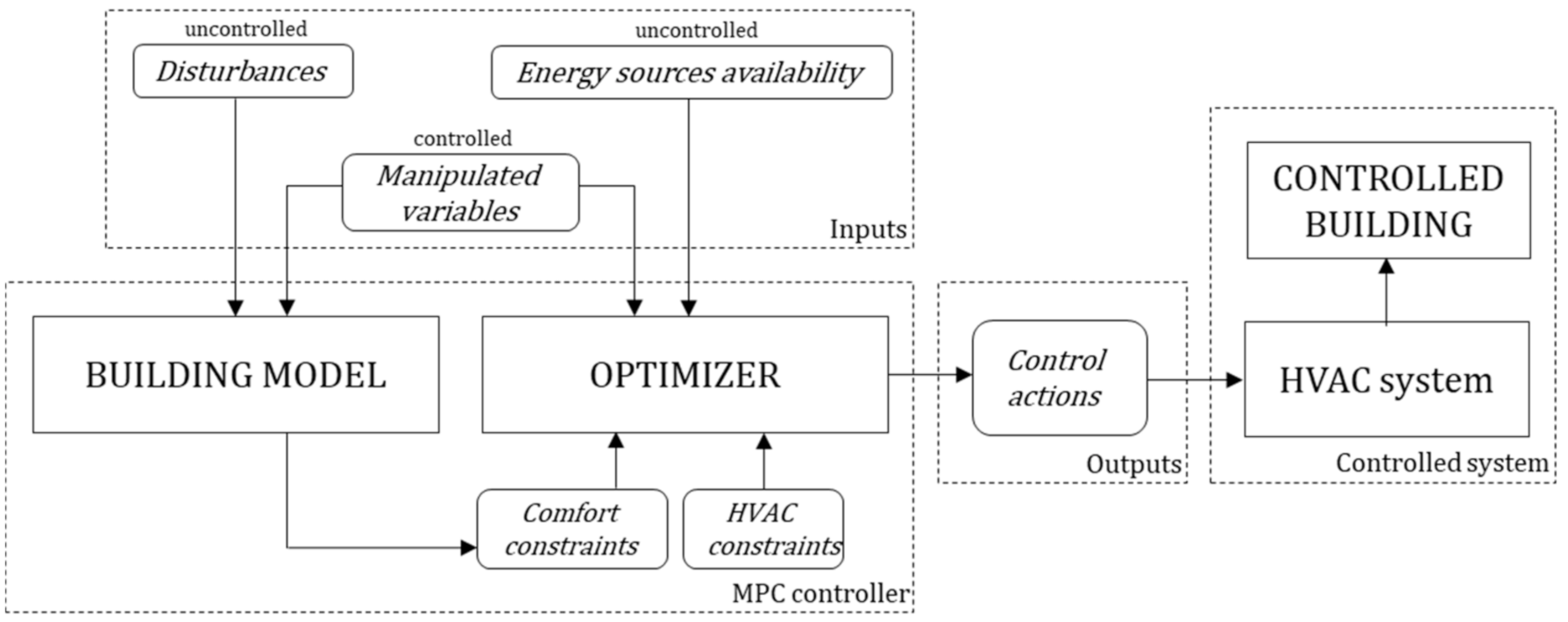
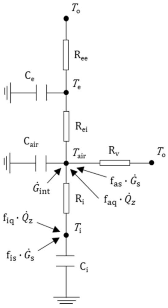
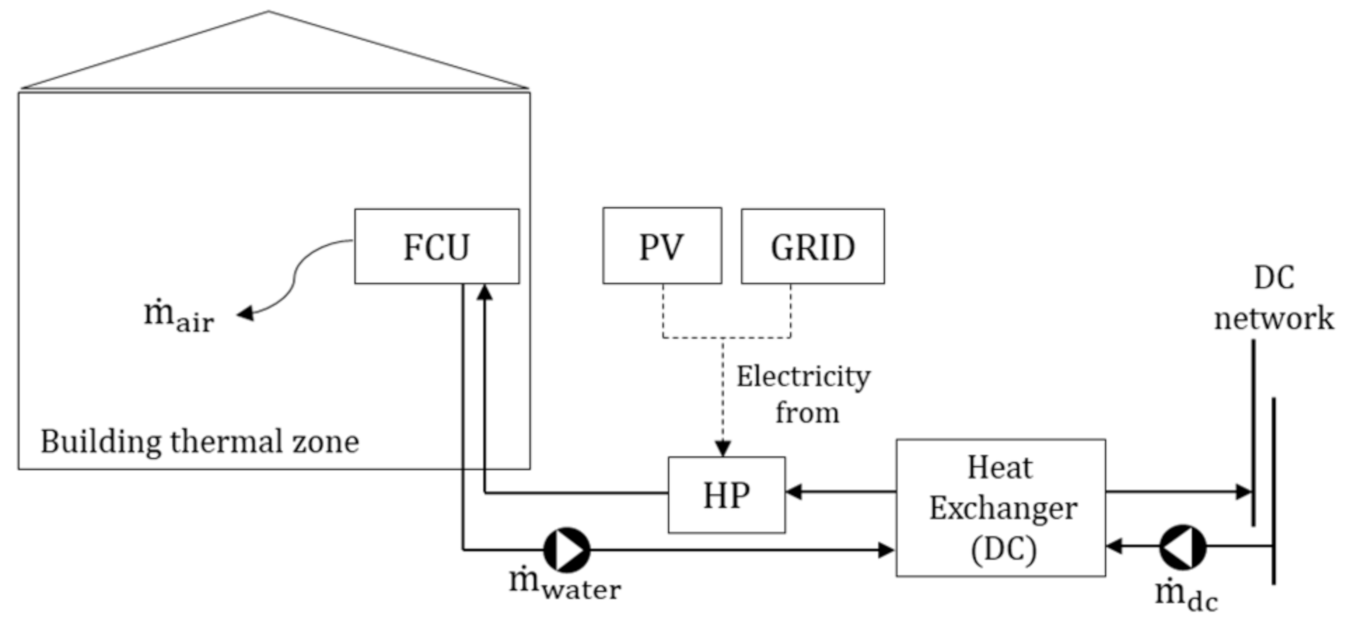
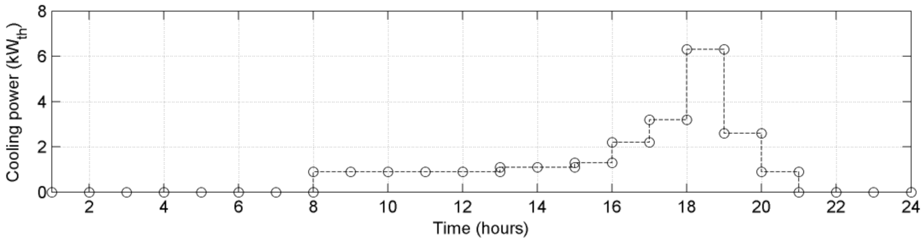
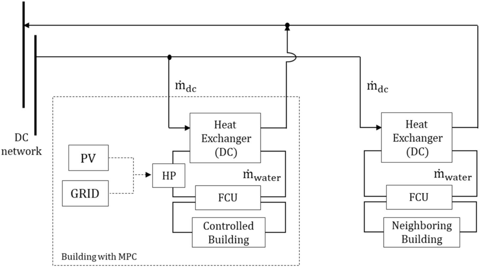
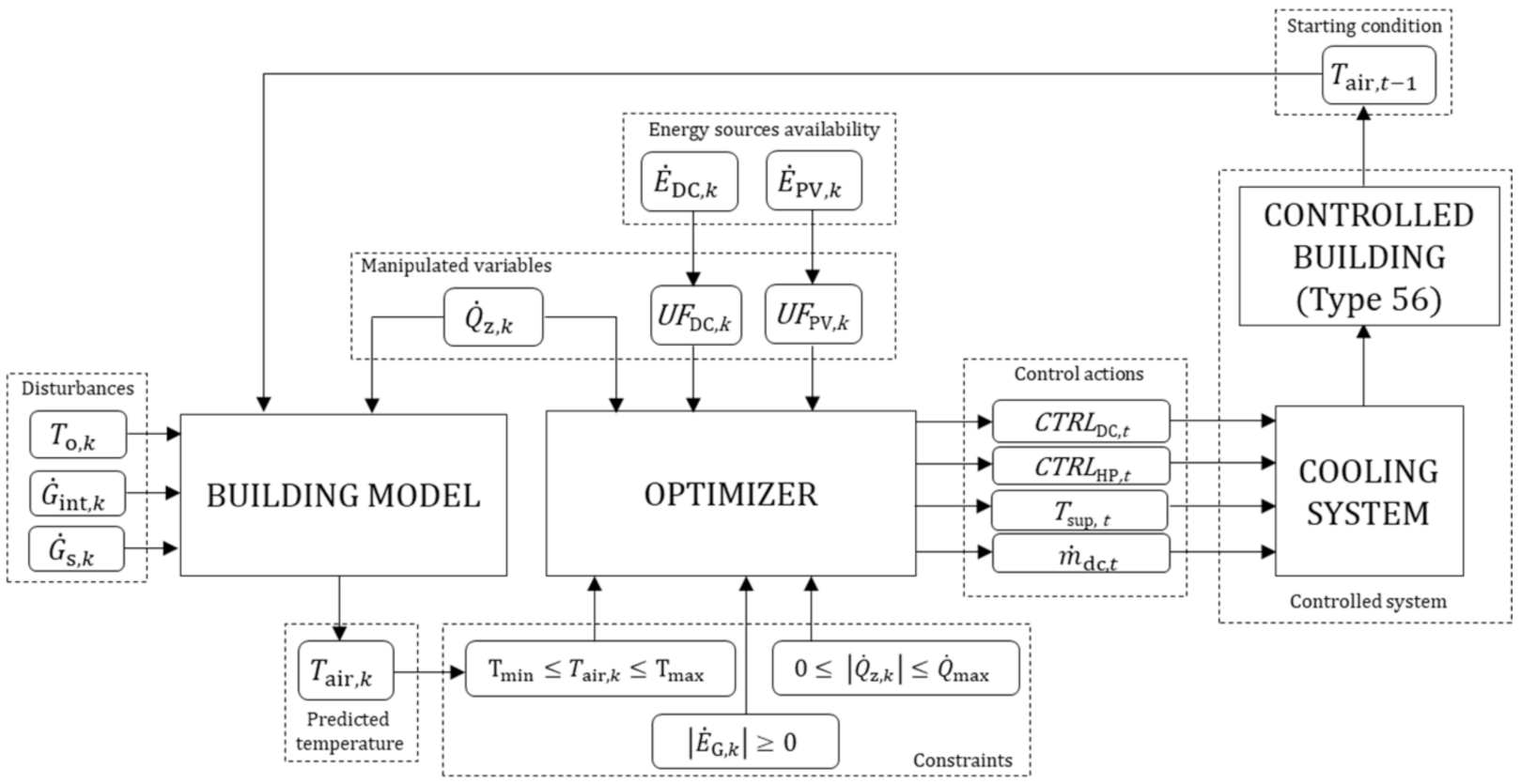
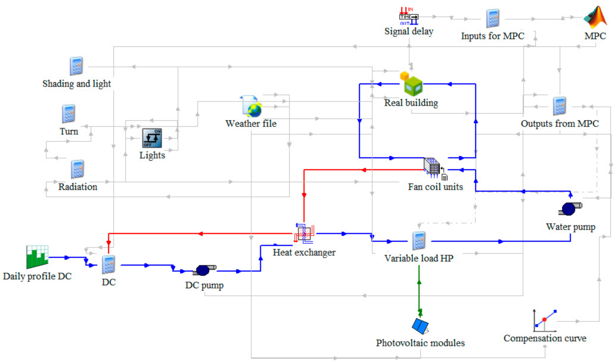
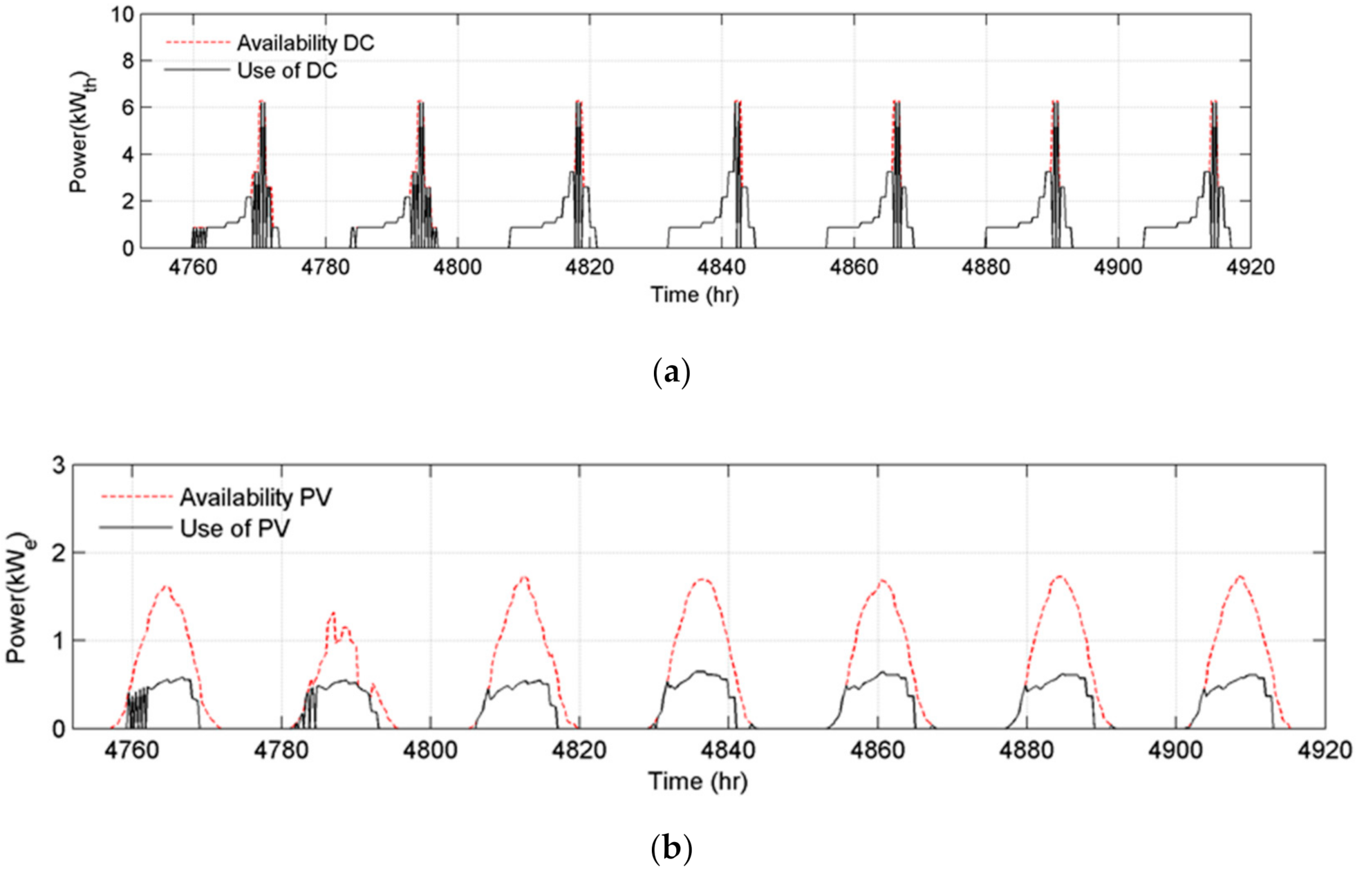
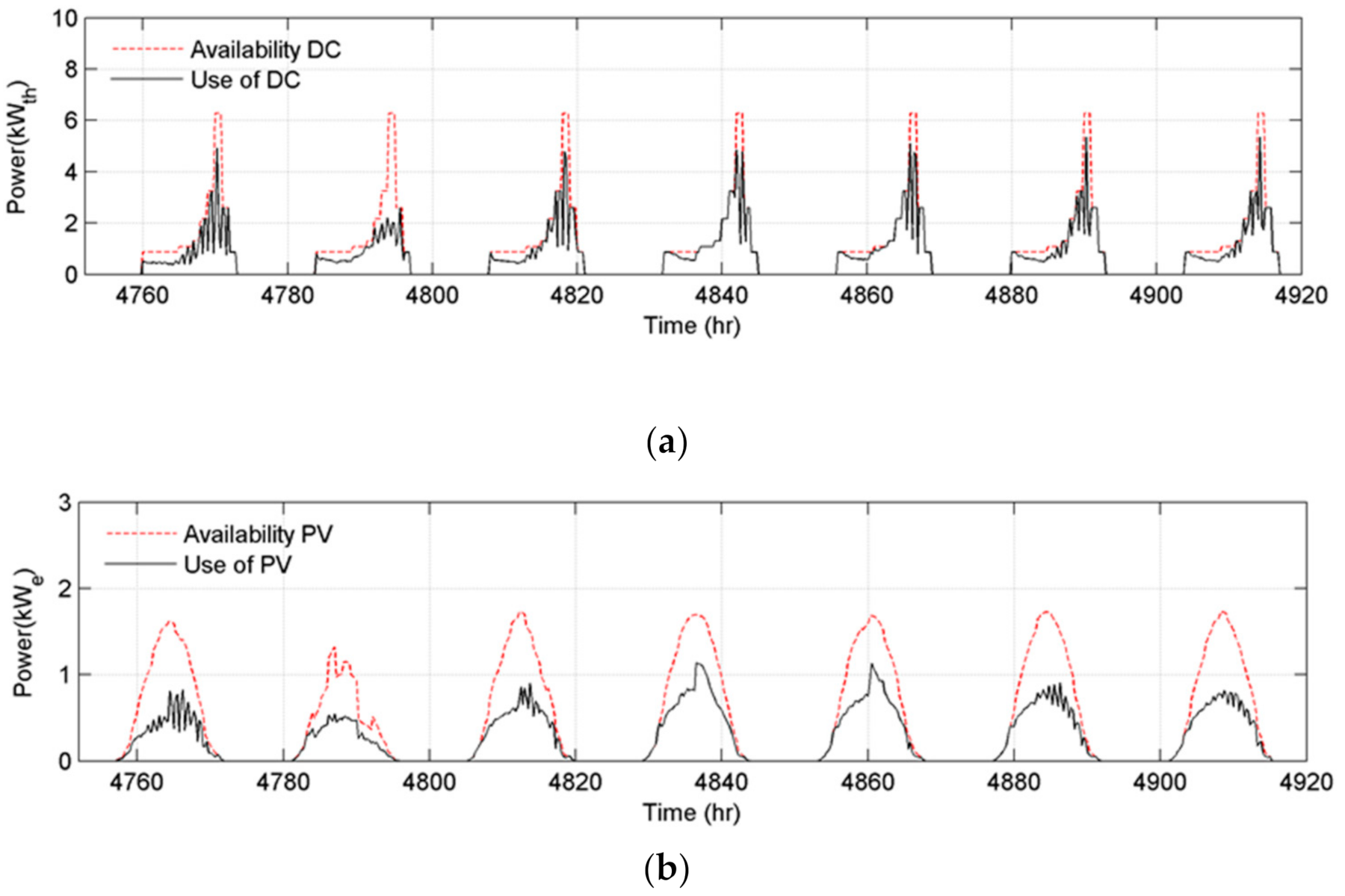
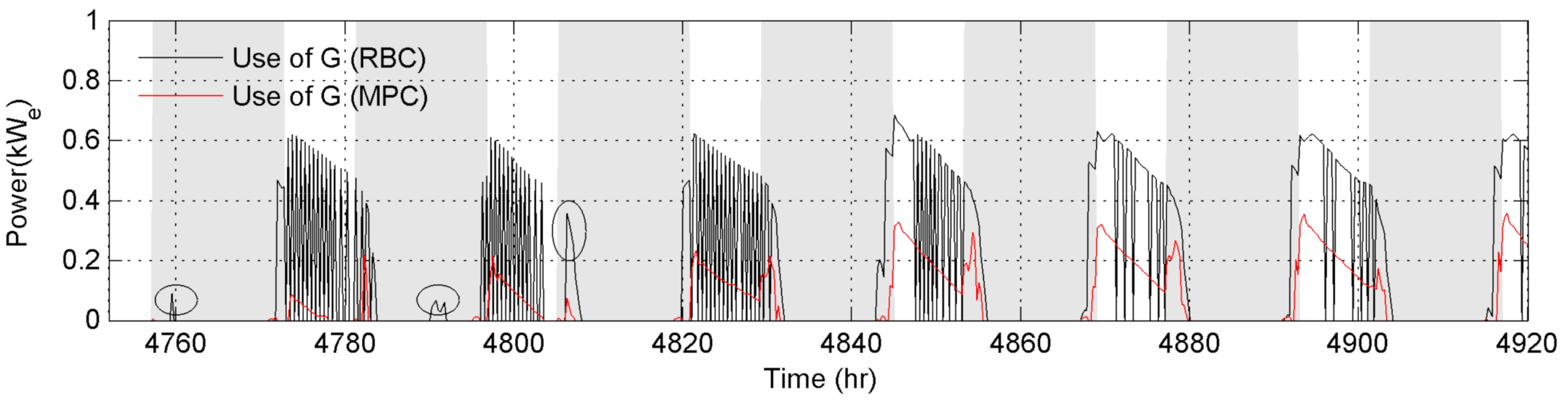
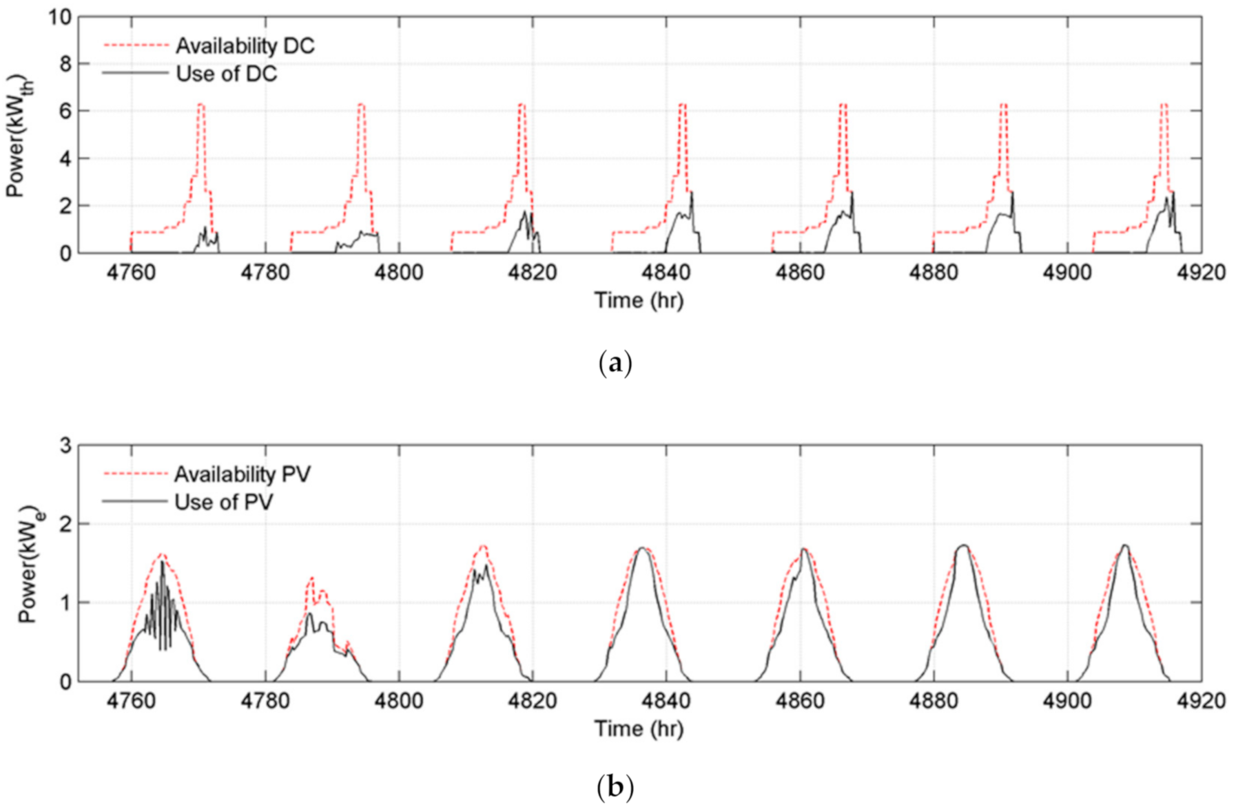
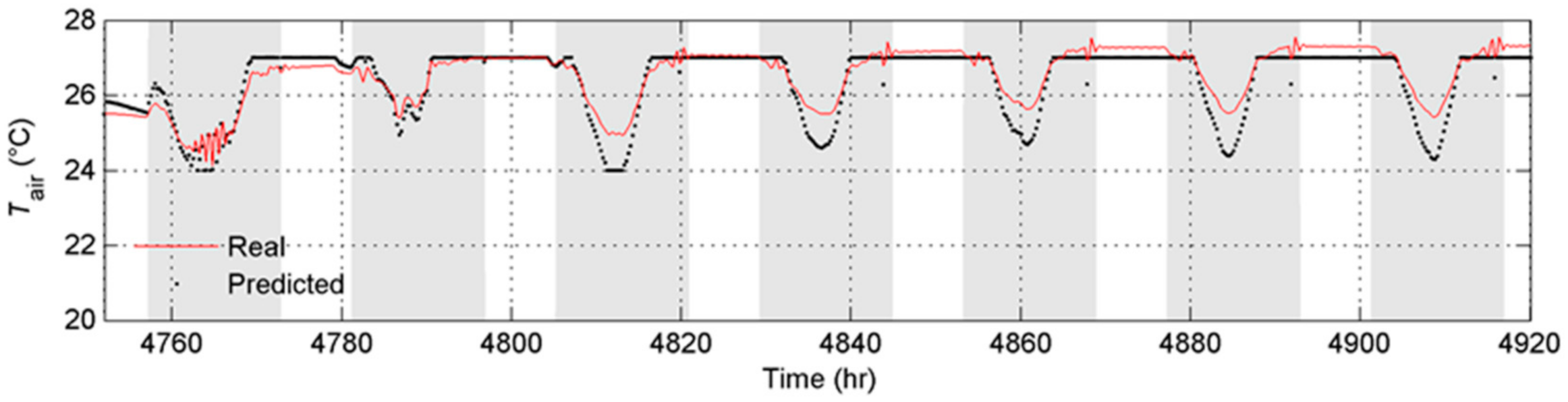
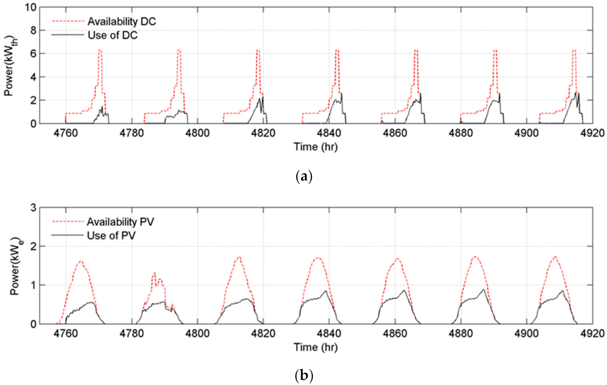
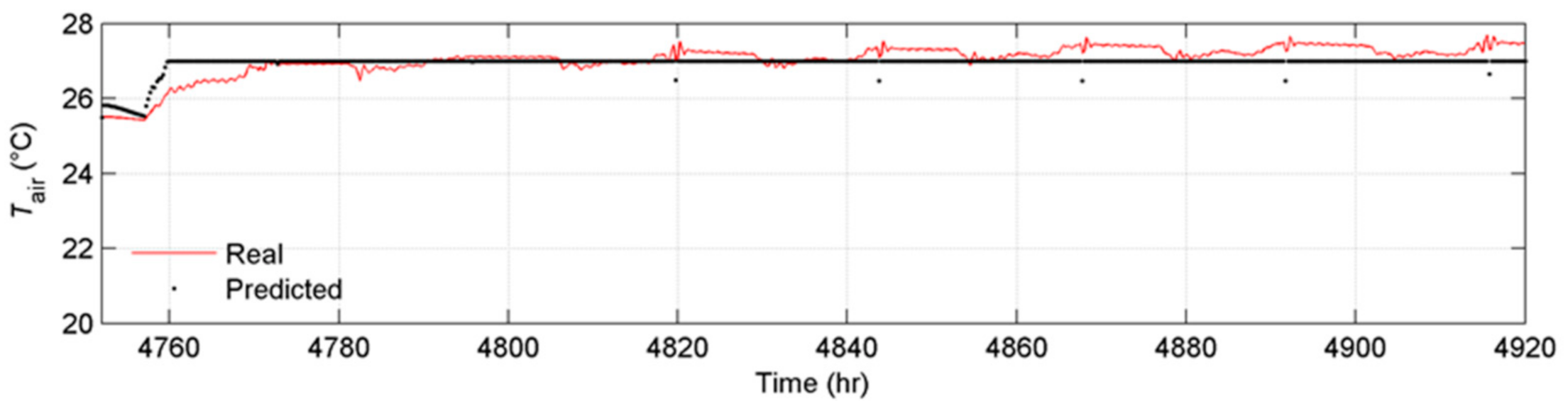
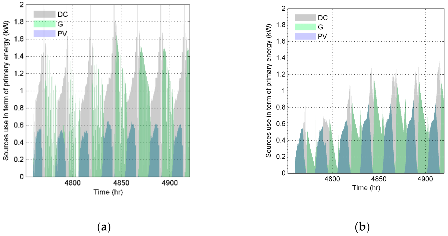
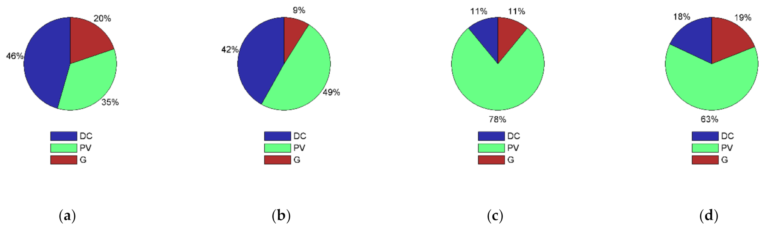
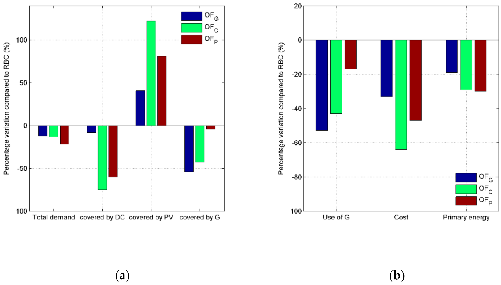
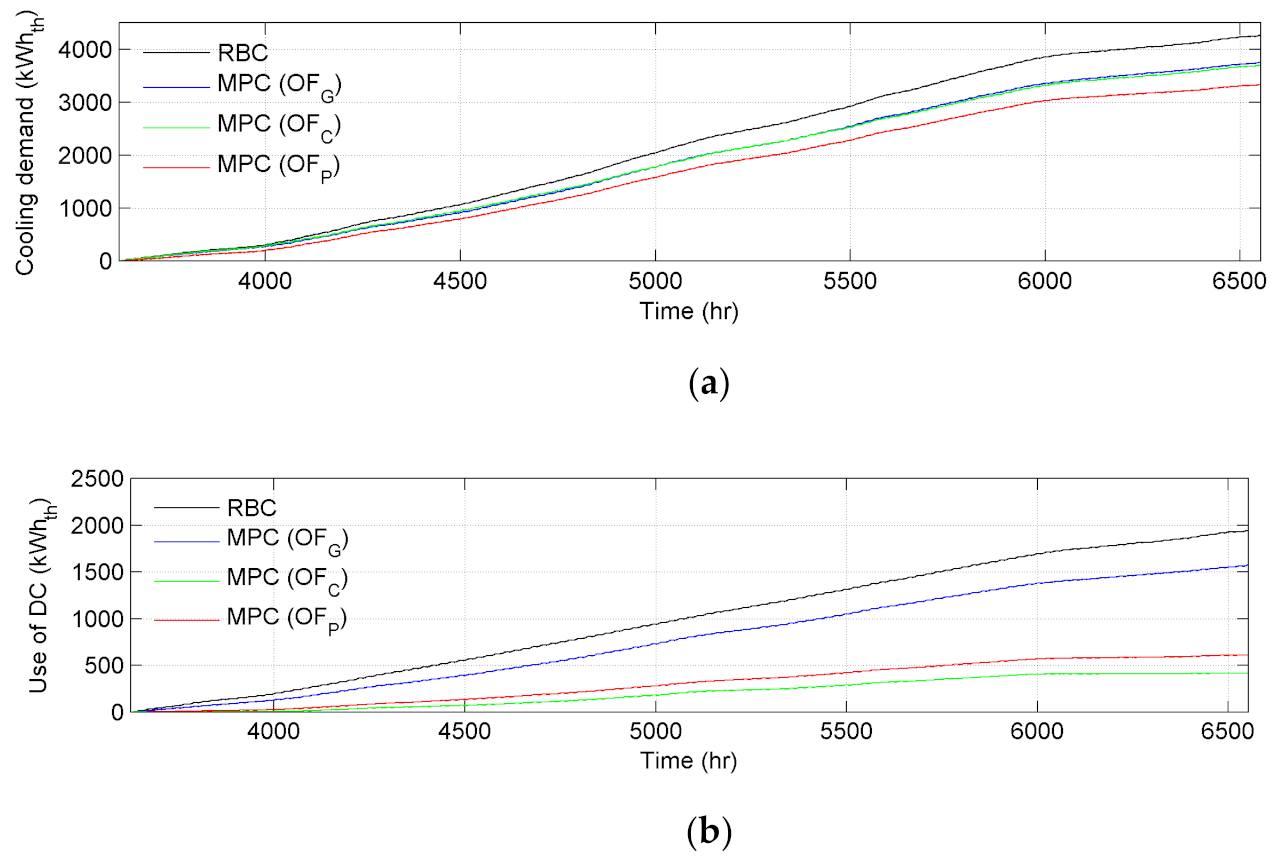
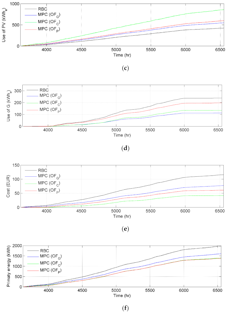
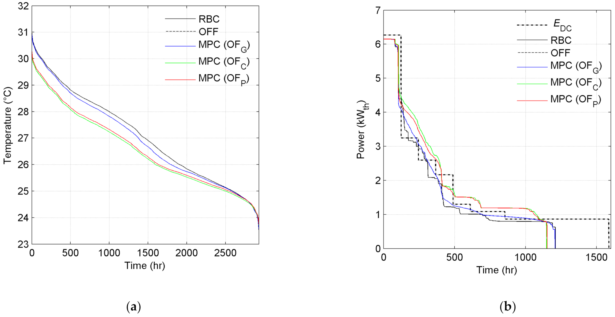
Table 1.
U-values (W m−2 K−1) and surface (m2) for each part of the building envelope. Developed from [22].
Table 1.
U-values (W m−2 K−1) and surface (m2) for each part of the building envelope. Developed from [22].
| Property | External Walls | Celing | Floor | Windows |
|---|---|---|---|---|
| U-values | 0.34 W m−2 K−1 | 0.28 W m−2 K−1 | 0.33 W m−2 K−1 | 2.20 W m−2 K−1 |
| Surface | 223.3 m2 | 96.4 m2 | 96.4 m2 | 23.3 m2 |
Table 2.
RC thermal network parameters.
(MJ K−1) | (MJ K−1) | (MJ K−1) | (KW−1) | (KW−1) | (KW−1) | (KW−1) | fas | faq | fis | fiq |
|---|---|---|---|---|---|---|---|---|---|---|
| 0.74 | 44.1 | 69.5 | 0.0107 | 0.0018 | 0.0068 | 0.0026 | 0.5 | 0.8 | 0.5 | 0.2 |
Table 3.
Design values for the cooling system sizing.
| Quantity | Water | Glycolate Water |
|---|---|---|
| Flow rate | 0.30 kg s−1 | 0.24 kg s−1 |
| Supply temperature | 7 °C | −5 °C |
| Temperature difference between supply and return | 5 °C | 7 °C |
Table 4.
Energy and cost performance with the RBC for the whole cooling season.
| Quantity | Value |
|---|---|
| Total cooling demand (kWhth) | 4263 |
| Cooling demand covered by DC (kWhth) | 1944 |
| Cooling demand covered by HP (kWhth) | 2319 |
| Total electricity demand (kWhe) | 665 |
| Electricity demand covered by PV (kWhe) | 426 |
| Electricity demand covered by G (kWhe) | 239 |
| Total energy cost (EUR) | 116 |
| Total primary energy consumption (kWh) | 1977 |
Publisher’s Note: MDPI stays neutral with regard to jurisdictional claims in published maps and institutional affiliations. |
© 2021 by the authors. Licensee MDPI, Basel, Switzerland. This article is an open access article distributed under the terms and conditions of the Creative Commons Attribution (CC BY) license (http://creativecommons.org/licenses/by/4.0/).
Share and Cite
MDPI and ACS Style
Mugnini, A.; Coccia, G.; Polonara, F.; Arteconi, A. Energy Flexibility as Additional Energy Source in Multi-Energy Systems with District Cooling. Energies 2021, 14, 519. https://0-doi-org.brum.beds.ac.uk/10.3390/en14020519
AMA Style
Mugnini A, Coccia G, Polonara F, Arteconi A. Energy Flexibility as Additional Energy Source in Multi-Energy Systems with District Cooling. Energies. 2021; 14(2):519. https://0-doi-org.brum.beds.ac.uk/10.3390/en14020519
Chicago/Turabian StyleMugnini, Alice, Gianluca Coccia, Fabio Polonara, and Alessia Arteconi. 2021. "Energy Flexibility as Additional Energy Source in Multi-Energy Systems with District Cooling" Energies 14, no. 2: 519. https://0-doi-org.brum.beds.ac.uk/10.3390/en14020519
Note that from the first issue of 2016, this journal uses article numbers instead of page numbers. See further details here.