Prediction of Refracturing Timing of Horizontal Wells in Tight Oil Reservoirs Based on an Integrated Learning Algorithm

Abstract

Refracturing technology can effectively improve the EUR of horizontal wells in tight reservoirs, and the determination of refracturing time is the key to ensuring the effects of refracturing measures. In view of different types of tight oil reservoirs in the Songliao Basin, a library of 1896 sets of learning samples, with 11 geological and engineering parameters and corresponding refracturing times as characteristic variables, was constructed by combining numerical simulation with field statistics. After a performance comparison and analysis of an artificial neural network, support vector machine and XGBoost algorithm, the support vector machine and XGBoost algorithm were chosen as the base model and fused by the stacking method of integrated learning. Then, a prediction method of refracturing timing of tight oil horizontal wells was established on the basis of an ensemble learning algorithm. Through the prediction and analysis of the refracturing timing corresponding to 257 groups of test data, the prediction results were in good agreement with the real value, and the correlation coefficient R² was 0.945. The established prediction method can quickly and accurately predict the refracturing time, and effectively guide refracturing practices in the tight oil test area of the Songliao basin.

1. Introduction

Tight oil exploration has broad prospects and is a key component of unconventional oil and gas exploration and development worldwide, with huge production potential [1,2]. Horizontal well volume fracturing is a key technology for scale benefit development of tight reservoirs [3,4,5]. Due to the influence of geological conditions, engineering conditions and working systems, there are some problems with horizontal well fracturing, such as a short effective period of stimulation and low recovery rate of single wells [6]. Refracturing technology is an effective way to restore single well production and extend the stable production cycle [7,8,9,10]. Refracturing timing refers to the interval between refracturing and primary fracturing of a production well [11]. The determination and accurate prediction of optimal refracturing timing are of great guiding significance for the macro-deployment, economic decision making and fracturing design of oilfields [12]. Many scholars have carried out a large number of studies on the determination of refracturing timing. Zhang [13] and Da [14] determined refracturing timing based on the formation time of stable stress inversion zones by analyzing changes in stress fields during fracture propagation. Yan [15], Udegbe [16], and R.D. Brier [17] analyzed well test curves or productivity decline curves and determined the time of hydraulic fracture failure as the time of refracturing. Oruganti [18] and Yu [19] compared the relationship between the time of refracturing and the effect of oil increases in multiple production wells and optimized the best time for reconstruction. Tavassoli [20], Guo [12] and Pang [11] set different refracturing timing conditions to carry out numerical simulations of production capacity prediction, and then optimized refracturing timing. Although previous research results have contributed a lot to the determination of refracturing timing for horizontal wells, these research results are only applicable to specific production wells and cannot be scientifically extended to other horizontal wells. Moreover, these methods require high economic costs and time cycles. Through technical investigation, it can be concluded that the stress field analysis method, dynamic analysis method and field statistics method cannot accurately quantify the timing of refracturing. The numerical simulation method takes the accumulated oil production within the same production time as the evaluation index. Although the timing of refracturing can be quantitatively optimized, it does not take the effect of the effective period of the measure into account, so it cannot accurately reflect the stimulation effect of the refracturing measure. In short, there is no suitable method to quickly and accurately predict the refracturing timing of horizontal wells on a large scale.

In the face of a large amount of fracturing well data, data analysis technology is getting a lot of attention [21,22,23,24]. When the time of refracturing is taken as the target parameter after quantitative characterization treatment, there should be a complex nonlinear relationship between it and the geological and engineering parameters of horizontal wells. However, machine learning methods have obvious advantages in dealing with nonlinear problems and predicting parameters [25].

In view of this, this study aims to present a prediction model of refracturing time from the perspective of technical economics; the time of refracturing is quantitatively represented, and the geological and engineering parameters of horizontal wells are taken as input data, while the time of refracturing is taken as output data, so as to construct a prediction model of refracturing timing based on machine learning methods.

2. Characterization of Refracturing Timing Parameters

With reference to the oilfield measure validity evaluation method, the horizontal well refracturing measure validity is defined as the time after the implementation of refracturing in which the daily oil production decreases to the level seen before the measure was applied. On this basis, the cumulative increase of oil during the effective period of the measure is the increase of output.

By using the numerical simulation method and referring to the physical characteristics of the target reservoir, a refracturing capacity prediction model was established to calculate increased production under different refracturing timings. As shown in Figure 1a, under different refracturing timing conditions, daily oil production can be effectively restored in the short term, and the stimulation effect of refracturing is obvious. Moreover, the earlier the refracturing, the earlier the economic benefit will be from the perspective of the whole life cycle. However, as can be seen from Figure 1b, with the increase in refracturing timing, the later the refracturing and the higher the oil increase—but the trend increase gradually becomes significantly slower. In a word, early refracturing is greatly affected by measures to increase productivity, and late refracturing results are relatively small. Therefore, the economic limit of oil well exploitation needs to be considered to further determine the most suitable time for horizontal well refracturing.

During the stage of steady decline, horizontal wells have the economic limit of daily production. In particular, this refers to the stable daily production of a single well that meets the minimum profit level under the conditions of current oil price and cost. When the daily oil production of horizontal wells during the stable production period is lower than the economic limit of daily production, the horizontal wells do not reach the economic development conditions, and so relevant stimulation measures should be carried out. Therefore, it is defined as the reasonable time for refracturing to be carried out when the daily oil production level drops to the economic limit following the initial fracturing of the horizontal wells. At this time, refracturing can not only ensure the fracturing effect and economic benefits, but also enable the wells’ production to take over the stimulation in time [26].

Considering the law of production decline of tight oil, scholars deduced the calculation formula of economic limit daily production [27] by integrating the investment in production capacity construction, operating costs of oil recovery, crude oil price, payback period of investment and other factors.

$$q_{\min }=\frac{\left(I_{\mathrm{D}}+I_{\mathrm{B}}\right)}{0.0365{\tau }_0\left({\displaystyle \sum _{t=1}^{{\mathrm{T}}_0}\frac{d_{\mathrm{o}}\left(P_{\mathrm{o}}-M-V_{\mathrm{o}}\right)}{{\left(1+i\right)}^t}}+{\displaystyle \sum _{t={\mathrm{T}}_0+1}^{\mathrm{T}}\frac{d_{\mathrm{o}}\exp \left[-D_i\left(t-{\mathrm{T}}_0\right)\right]\left\{P_{\mathrm{o}}-M\exp \left[-D_i\left(t-{\mathrm{T}}_0\right)\right]-V_{\mathrm{o}}\right\}}{{\left(1+i\right)}^t}}\right)}$$

(1)

where q_min is the economic limit of daily oil production (t/d); I_D is horizontal well drilling investment (including perforation, fracturing, etc.), 10,000 yuan/well; I_B is the surface investment for horizontal wells, 10,000 yuan/well; τ₀ is the oil recovery rate; d_o is the commodity rate of crude oil; T is the development evaluation period, year; T₀ is stable production period, year; P_o is the selling price of crude oil, yuan/t; M is the operating cost per ton of oil, yuan/t; V_o is the comprehensive tax, yuan/t; D_c is the annual comprehensive decline rate of oilfield; and i is the discount interest rate, %.

By substituting the relevant economic accounting data of target field into Formula (1), it can be calculated that the economic limit daily output of horizontal wells in target reservoir is 3.04 t/d. On this basis, the time experienced by each horizontal well in the demonstration area when the daily oil production level decreases to 3.04 t/d after fracturing is counted, and the quantitative characterization of the time of refracturing in the target reservoir is completed.

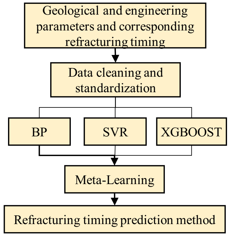
3. Principle and Method of Refracturing Timing Prediction

Different geological parameters, fracturing scale, and the operating system all affect the production of tight horizontal wells—thus affecting the timing of refracturing. There are complex nonlinear relationships between geological and engineering factors and refracturing effect in horizontal wells [28]. It is difficult to establish the quantitative relationship between geological and engineering parameters and refracturing timing; however, machine learning techniques have obvious advantages in the treatment of a large amount of nonlinear, high dimension data [29]—so it can be used to construct a refracturing timing prediction model influenced by multicomponent factors.

In view of this, a prediction model of refracturing timing based on machine learning methods was constructed, in which the geologic and engineering parameters were the input item, while refracturing timing was the output item. When the sample set was constructed, the measured production well data and a large amount of numerical simulation data were fully collected to support the subsequent learning and generalization process.

When the sample set was constructed, the measured production well data and a large amount of numerical simulation data were fully collected to support the subsequent learning and generalization process; the machine learning algorithm with good predictive effect was optimized, the model prediction accuracy was further improved through integrated learning methods, and the model was evaluated by uncertainty analysis.

Three machine learning algorithms widely used in the field of artificial intelligence were selected for modeling [21,30,31]. In this section, each employed machine learning algorithm is briefly described. In the process of model training and testing, the parameters of the algorithm were adjusted, and the prediction effect of each model was compared. The integrated learning idea was introduced, and the basic model was trained [25,32]. Finally, the comprehensive prediction model was generated to further strengthen the prediction accuracy of the model.

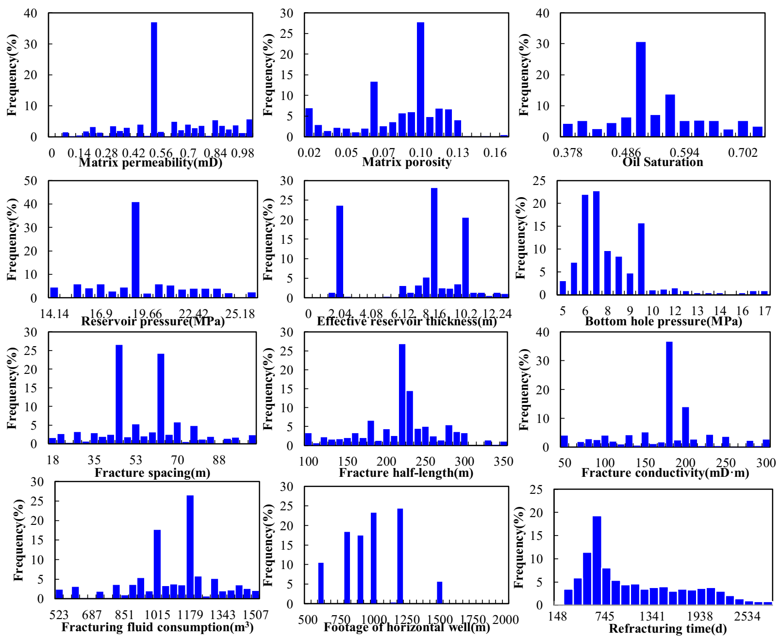
3.1. Sample Set Construction

In machine learning technology, the selection and construction of learning samples directly affect the prediction effect of the model. Based on geological data, fracturing design monitoring, dynamic production and other data of horizontal wells of tight oil in the Songliao Basin, geological and engineering parameters of horizontal wells in different blocks and their corresponding refracturing timing values were statistically collected to form an initial learning sample set. Specific input and output data are shown in

Table 1. Prediction input and output of the model.

Input		Output
Geological properties	Matrix permeability	Refracturing timing
	Matrix porosity
	Reservoir pressure
	Effective reservoir thickness
	Oil saturation
Engineering properties	Fracture half-length
	Fracture conductivity
	Fracture spacing
	Fracturing fluid consumption
	Footage of horizontal well
	Bottom hole pressure

.

Due to the limited number of on-site production wells and the fact that a considerable number of new horizontal wells drilled have not yet reduced their production capacity to the economic limit of daily production, the timing of refracturing cannot be counted. Therefore, if the actual data of the field is taken as learning samples alone, the quantity and quality are far from meeting the training sample requirements of machine learning.

To this end, a large number of horizontal well development geological models were built for different types of tight oil reservoirs in the target block, and 2000 geological schemes with average permeability of (0.05~1.2) × 10⁻³ µm² were generated by a sequential Gaussian generator for model permeability. Permeability images of some geological models are shown in Figure 2. The porosity value was assigned according to the pore permeability fitting relationship of the actual reservoir. Other geological and engineering parameters were generated by calling algorithms to generate 2000 groups of random combination schemes for productivity simulation [5,33]. Finally, the geological and engineering parameters of each scheme and the corresponding refracturing time were collected and counted. On this basis, the actual statistical data of well production was added to form a learning sample set.

A total of 2000 sets of mathematical model scheme samples and 48 sets of actual data samples were collected. The minimum, maximum and average refracturing time in the collected sample sets was 148 d, 2892 d and 717 d, respectively, and the refracturing time was mainly concentrated between 400–800 d. For the constructed learning samples, there will be some noise data due to the accuracy of statistical data and errors in the numerical simulation. Based on the actual engineering experience, the outlier data were eliminated and replaced before the model training by using the relationships between the known parameters. Finally, 1896 groups of sample data were collected for subsequent algorithm training and testing.

In the process of model training, in order to avoid the influence of data span, learning samples were standardized to convert them into a range of 0–1, which is convenient for the application of machine learning algorithms. Logarithmic conversion was used to deal with the timing value of refracturing, so that it conforms to the characteristics of normal distribution to a certain extent (Figure 3). The continuous characteristic distribution map of each input parameter was as follows (Figure 4).

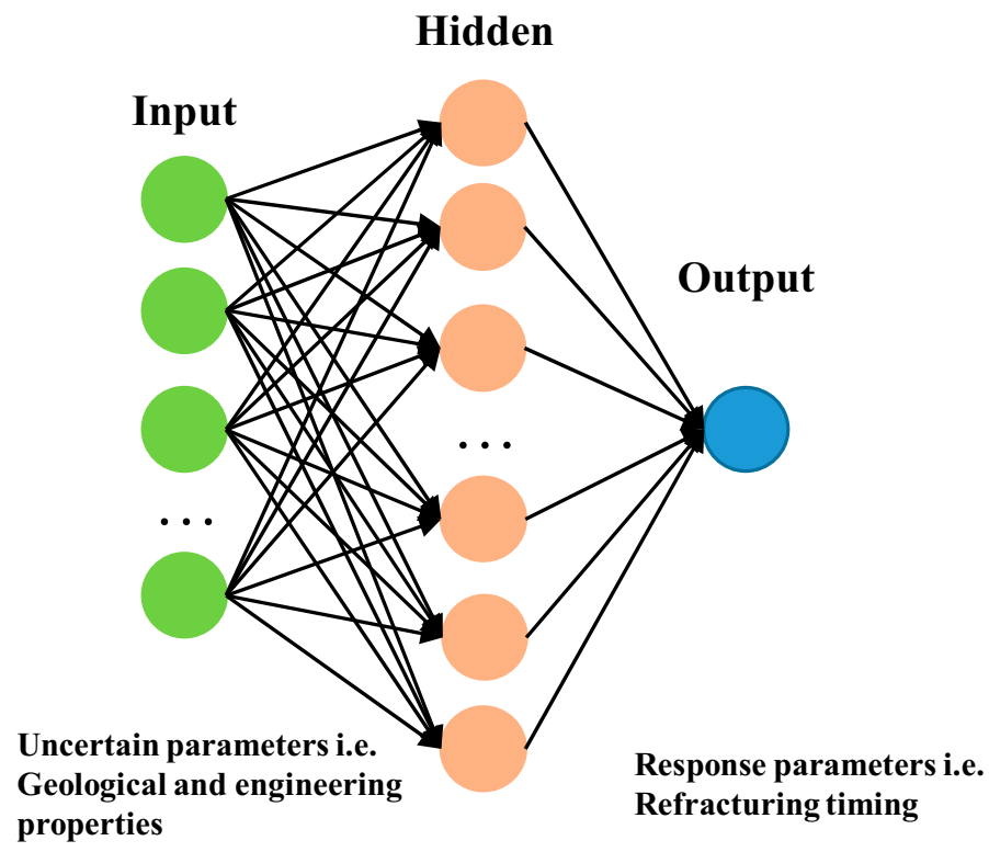
3.2. Artificial Neural Network Algorithm

Artificial neural networks, proposed by Rumelart and McClelland, have been widely used in the oil and gas industry as machine learning algorithms [31,34,35,36]. Neurons in the network included an input layer, output layer and several hidden layers (Figure 5). In this experiment, the Bayesian regularization algorithm was used to train the model. Through the training of sample data, the network weights and thresholds were continuously modified to make the error function decrease along the negative gradient direction and approximate the expected output. Finally, the number of nodes in the hidden layer of the neural network optimization was six.

However, the error function value is prone to gradient explosion and gradient collapse in the process of reverse propagation, so the training effect is not ideal. At the same time, due to the problem of sample dependence, artificial neural networks have over-fitting defects. Therefore, the generalization of the neural network algorithm needs to be verified in view of specific application problems.

3.3. Support Vector Machine Regression Algorithm

Support vector machines (SVMs) are kernel-based dichotomy algorithms, which map all data to the high-order vector space and find a hyperplane in the high-order N-dimensional data space, making the complex data linearly separable [21,37]. In order to solve the problem of over-fitting, Vapnik et al. introduced the SVM classification-insensitive loss function L(y,f(x)) [38], thus obtaining the support vector machine regression (SVR) algorithm. The core idea of the SVR algorithm is to find a separating hypersurface that can correctly divide the training dataset, where the geometric interval between the dataset and the hyperplane is the largest. The SVR algorithm can be expressed as:

$$\min = \left\{\frac{1}{2}{‖\omega ‖}^2+C{\displaystyle \sum _{i=1}^l{l}_{\epsilon }\left(f\left(\mathrm{x}\right) - y_i\right)}\right\}$$

(2)

Since nonlinear problems are often encountered in practical applications, relaxation variables are introduced to simplify the calculation:

$$\min = \left\{\frac{1}{2}{‖\omega ‖}^2+C{\displaystyle \sum _{i=1}^l{\xi }_i+{\xi }_i^{\ast }}\right\}$$

(3)

where C is the penalty coefficient, a greater C means a greater penalty, and ζ_i, ζ^*_i is the relaxation factor.

On this basis, the kernel function K(x_i,x_j) is introduced to simplify the calculation process; its expression is:

$$K\left(x_i,x_j\right)={\mathrm{e}}^{\frac{-{(x_i-x_j)}^2}{2{\sigma }^2}}{=\mathrm{e}}^{\left(-gamma\times {(x_i-x_j)}^2\right)}$$

(4)

where the gamma parameter implicitly determines the distribution of the data mapped to the new feature space. If the gamma setting is too large, the Gaussian distribution will only act near the support vector samples. At this time, the accuracy of the training set is very high, but the classification and prediction of unknown samples are poor.

When the kernel function meets the Mercer theorem, it can effectively solve high-dimensional nonlinear problems, and the final classification decision function expression is:

$$f(\mathrm{x})=\mathrm{sgn}({\displaystyle \sum _{i=1}^l{\alpha }_i^{\ast }{y}_{i}K\left(x_i,x\right)} + b^{\ast })$$

(5)

According to the algorithm structure characteristics of the support vector, the idea of parameter optimization of the support vector machine algorithm is to find the optimal penalty coefficient C and the gamma parameter combination in the kernel function when giving the parameter range of C and gamma.

3.4. XGBoost Regression Algorithm

XGBoost is a boosting tree model, which implements a boosting algorithm. The core idea of XGBoost is to integrate a number of weak classifiers into a strong classifier, which integrates many tree models together and effectively avoids the over-fitting problem of tree models. It has obvious advantages in regression accuracy [30,39], and its model expression can be expressed as:

$${\widehat{y}}_i={\displaystyle \sum _{k=1}^K{f}_k\left(x_i\right)}$$

(6)

where f_k is the k_TH tree model, y_i is the predicted result of sample x_i, and the learning process loss objective function is set as follows:

$$\mathrm{O}b{j}^{\left(t\right)}={\displaystyle {\sum }_{i=1}^{n}l\left(y_i,{\widehat{y}}_i^{\left(t-1\right)}+f_t\left(x_i\right)\right)}+ \Omega \left(f_t\right) +\mathrm{constant}$$

(7)

where l is the loss function, satisfying the second-order differentiable; and Ω(f_t) as the regularization item, its specific form can be expressed as:

$$\Omega \left(f\right) =\gamma T+\frac{1}{2}\lambda {‖\omega ‖}^2$$

(8)

where T is the number of branches in the decision tree algorithm; and ω is the branches parameters vector.

After Taylor’s second-order expansion of Formula (7), the updated objective function can be expressed as:

$$\left\{\begin{array}{l}\mathrm{O}b{j}^{\left(t\right)}\approx {\displaystyle {\sum }_{i=1}^{n}l\left(y_i,{\widehat{y}}_i^{\left(t-1\right)}+{\mathrm{g}}_i{f}_t\left(x_i\right)+\frac{1}{2}{h}_i{f}_t^2\left(x_i\right)\right)}+ \Omega \left(f_t\right) +\mathrm{constant}\\ {\mathrm{g}}_i={\delta }_{{\hat{y}}^{\left(t-1\right)}}l\left(y_i,{\widehat{y}}_i^{\left(t-1\right)}\right)\\ h_i={\delta }^2{}_{{\widehat{y}}^{\left(t-1\right)}}l\left(y_i,{\widehat{y}}_i^{\left(t-1\right)}\right)\end{array}\right.$$

(9)

where g_i and h_i are the first and second derivatives of loss function l at y^(t−1).

To avoid overfitting in the training process, the algorithm does not train all regression trees at the same time but adds decision trees in turn. Therefore, when adding t trees, the previous t − 1 tree has been trained, therefore $l\left(y_i,{\widehat{y}}_i^{\left(t-1\right)}\right)$ can be regarded as a constant oversight, while eventually, the objective function is simplified as:

$$\mathrm{O}b{j}^{\left(t\right)}\approx {\displaystyle {\sum }_{i=1}^n\left({\mathrm{g}}_i{f}_t\left(x_i\right)+\frac{1}{2}{h}_i{f}_t^2\left(x_i\right)\right)}+ \Omega \left(f_t\right) +\mathrm{constant}$$

(10)

The parameter optimization of the XGBoost regression algorithm involves multiple parameter combinations, and the conventional grid search optimization method needs to be optimized by traversing all parameters Therefore, the strategy of level-by-level parameter tuning is adopted to complete the algorithm optimization and to find the optimal parameter combination [28].

Therefore, the strategy of adjusting parameters step-by-step was used to optimize the algorithm, and the optimal combination of algorithm parameters was finally found. The specific optimization steps are as follows:

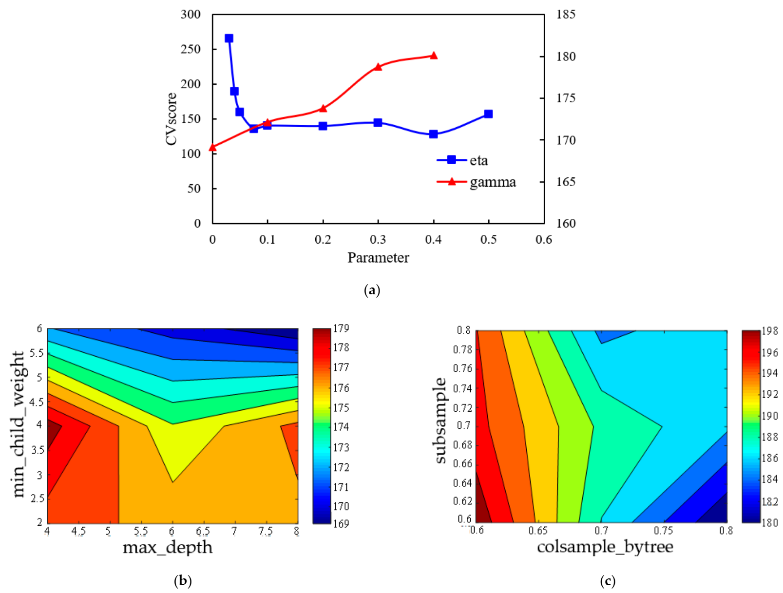
• According to conventional experience, a group of initial parameters was selected, and the number of decision trees was set as 50. On this basis, the depth of decision trees (max_depth) and node weights, namely, the regularization coefficient, (min_child_weight) were adjusted. The optimal parameter combination could be found by drawing a heat graph of the loss function with the tree depth and regularization coefficient.
• Adjust the gamma; this parameter determines when the loss function is split, and the smaller the parameter is, the smaller the risk of overfitting is. Therefore, under the premise of ensuring the rationality of the loss function, gamma was taken to be as small as possible.
• Adjust the sampling mode; these parameters mainly involve column sampling (colsample_bytree) and row sampling (subsample). In the same way, the best parameter combination could be found by drawing a heat map of the loss function with two parameters.
• Adjust the learning rate eta; the loss function was compared to complete the eta parameter optimization.

Finally, the maximum depth was 8, the minimum child weight was 6, the colsample bytree was 0.8, the subsample was 0.6, and the learning rate (eta) was 0.4. The change in damage function with parameters in the optimization process is shown in Figure 6.

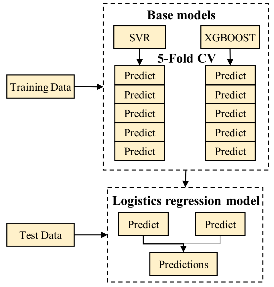
3.5. Integrated Learning Algorithm

Machine learning algorithms vary in training speed and prediction accuracy due to their different principles and algorithm structures. In addition, the optimal adaptability of each machine learning algorithm may be different under the premise of sample sets of different sizes [25,40]. On the other hand, it is difficult to further improve the prediction effect of a single algorithm model after parameter tuning optimization [41]. Integrated learning technology in the field of machine learning can aggregate regression prediction results from multiple single algorithms and produce comprehensive prediction results after fusion training, which further improves the model prediction effect [32,42,43]. Therefore, based on the prediction results of repeated fracturing timing of BP, SVR and XGBoost algorithms, the prediction effects of each algorithm model were compared and analyzed. The algorithm model with a good prediction effect was selected as the basic model of the fusion model. The prediction results of the basic model were taken as the meta-features, fed to the meta-learner, trained and evaluated by the fusion model, and finally, the comprehensive prediction model of repeated fracturing timing was obtained.

Figure 7 shows the workflow of the prediction method of refracturing timing. The integration process of ensemble learning algorithm will be described in detail in the next section of the article.

4. Algorithm Application and Analysis

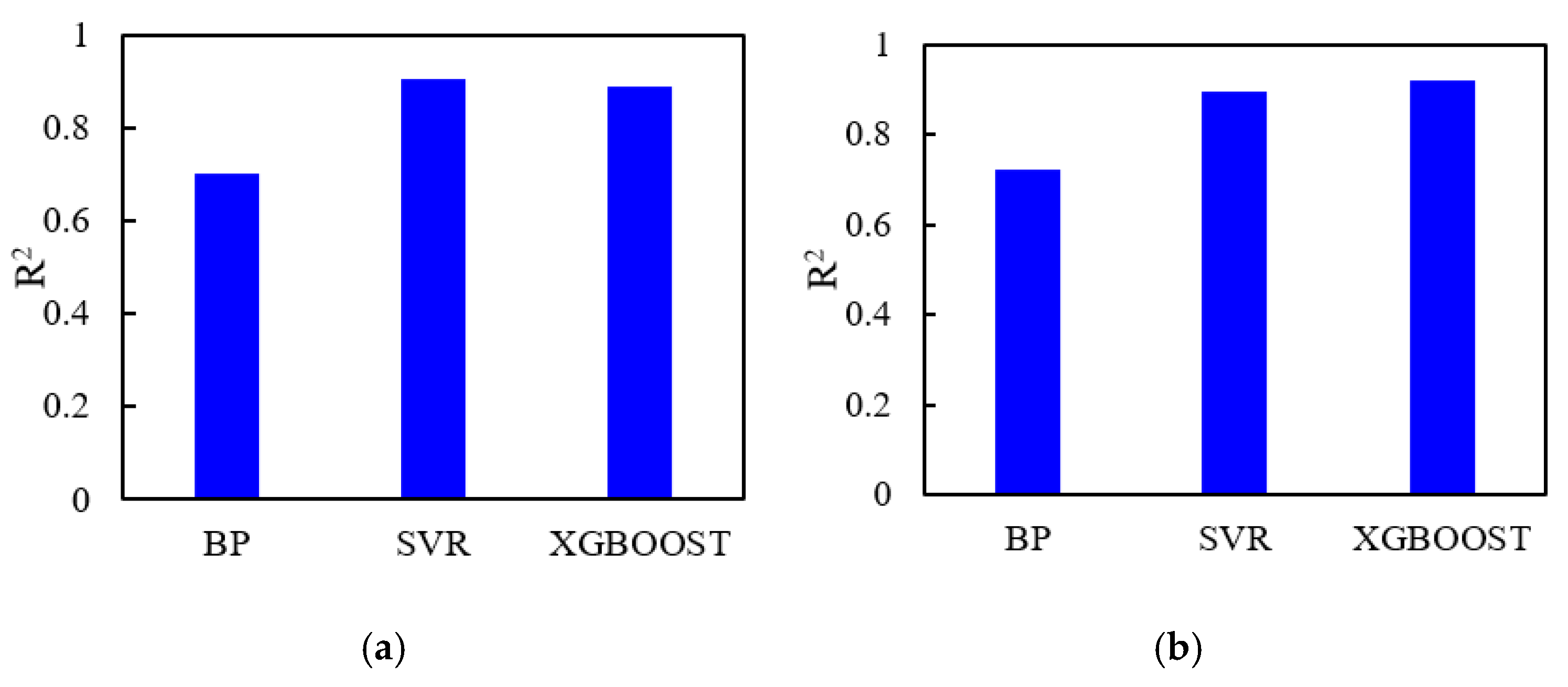
4.1. Application Evaluation Analysis of the Algorithm

During the training process, 90% of the sample set data was used to train, verify and test the model, and the remaining 10% of data was used to predict the model after training. Under the condition of different training sample numbers, three algorithms were used for model training and prediction respectively, and the prediction effect of the test set is shown in Figure 8. It can be concluded that when the number of learning samples was small (group 800), the prediction effect of SVR algorithm was the best, and the correlation coefficient R² between the predicted value and the real value of the model was 0.906. When the number of learning samples was large (1896 group), the XGBoost regression algorithm showed absolute advantages, and the correlation coefficient R² between the predicted value and the real value was 0.921. However, artificial neural networks are prone to over-fitting, so their generalization ability is poor. Under the conditions of different sample numbers, their prediction accuracy was lower than the other two algorithms, and the correlation coefficient was stable at about 0.7. Therefore, SVR and XGBoost regression are preferred as the basic models when building fusion prediction models using integrated learning algorithms.

During the integration learning process, the model stack method was used to blend the SVR and the XGBoost algorithm. The specific idea of this method is to divide the learning sample set according to a 9:1 ratio and train and predict the basic model, respectively, by using the strategy of 50-fold cross verification. In the process of cross-validation, each training sample will produce relative corresponding prediction results. Therefore, after the end of cross-validation cycle, the prediction results of the basic model B¹_train = (b₁,b₂,b₃,b₄,b₅)^T and B²_train = (b₁,b₂,b₃,b₄,b₅)^T can be obtained, and the prediction results of the basic model will be fed to the secondary model for regression. In the process of regression prediction, in order to prevent the occurrence of over-fitting, a relatively simple logistics regression model was selected to process the data, and finally the prediction results of the integrated learning model were obtained (Figure 9). By comparing the predicted results of the integrated learning model and the basic model, the correlation coefficient between the real value and the predicted value of the refracturing time in the test set was calculated, as shown in Figure 10.

From the analysis of Figure 8, it can be concluded that the correlation coefficient R² of the integrated learning algorithm based on a logistics regression model was the highest, up to 0.945. Compared with the prediction results of a single algorithm, the prediction accuracy of the model was further improved. The comparison curve between the real value of the refracturing time of some samples in the test set and the predicted value of the integrated learning algorithm is shown in Figure 11. It can be seen that the predicted value of the refracturing time fluctuated around the actual value with a small prediction error and a high degree of agreement with the field measurement and mathematical model data. Therefore, the established prediction method can replace the conventional numerical simulation workflow, quickly and accurately predict the refracturing time, and effectively guide field practice.

4.2. Field Implementation Effect

Taking well X34-X6 in the tight oil test area of the Songliao Basin as an example, a total of 9 clusters of fractures were designed and constructed during the initial fracturing process, with average fracture spacing of 100 m, fracturing fluid consumption of 14,400 m³, and fracturing sand addition of 460 m³. The initial average production after pressure was up to 30 t/d. Up to now, the average daily oil production was 3.07 t/d, close to the economic limit of daily production. By inputting geological and engineering parameters into the established prediction model, the predicted value of the time of repeated fracturing was 712 d, which is highly consistent with the actual value of 649 d.

On this basis, the method of refracturing with new fractures was adopted. A total of 15 clusters of fractures were designed and constructed. The designed fracture length was 300–400 m, the fracture height was 8–10 m, and the construction displacement was 5–6 m³/min. The dual-packer and single-clip staged fracturing technology was used to complete the construction, and the refracturing process was smooth. To the whole well was added 56 m³ ceramsite, 748 m³ quartz sand and 7673 m³ Guar gum fracturing fluid. After refracturing, the daily fluid level recovered to 31 t/d, and the daily oil level recovered to 10.2 t/d. The daily oil output reached 71.2% of that of the initial fracturing, and the cumulative oil increase was 3171.4 t, showing an obvious stimulation effect (Figure 12).

5. Conclusions

The results are shown below:

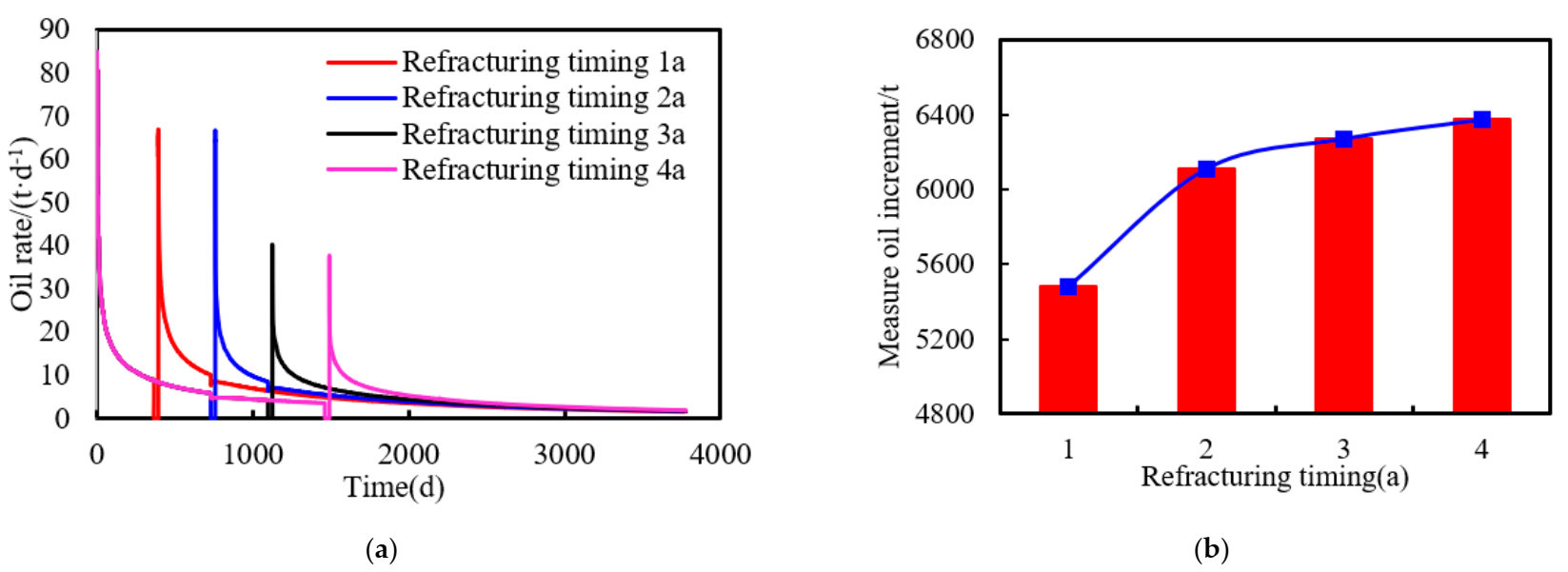
• Based on the increased production of horizontal wells with refracturing measures as the evaluation index, the law of the influence of refracturing timing on the stimulation effect was analyzed. Combined with the economic limit of tight oil horizontal wells, the economic limit daily production of horizontal wells was calculated, and the reasonable refracturing timing was quantitatively characterized.
• Using machine learning techniques to measure the geologic and engineering parameters of horizontal wells, with a total of 11 variables as input, the refracturing time as output, the comprehensive field measurements and a large number of numerical simulation data to construct the learning sample set, and noise reduction processing on the sample set, three kinds of modeling and prediction effect comparisons of machine learning algorithms were chosen; the results showed that the support vector machine and XGBoost regression algorithm of artificial neural network algorithm showed better generalization.
• Through integrated study of the depth of the stacking method, SVR and XGBoost were combined to build the dense oil refracturing horizontal well, based on the integrated study time prediction method. Using 257 groups to build a prediction model in a test set forecast result analysis, it was shown that, compared with a single algorithm model, the prediction accuracy was higher, and the actual and estimated values of the correlation coefficient R² were 0.945—alternative numerical simulation processes quickly predicted refracturing timing. The prediction model was used to predict the refracturing time of the X34-P6 well in the target reservoir, and the predicted results were in great agreement with the actual value.
• Having a high predictive accuracy, the integrated learning model can serve as a reliable tool for predicting refracturing time. It has high potential for being applied in macro decision making of horizontal well repeated fracturing.

References

1. Zheng, M.; Li, J.; Wu, X.; Wang, S.; Guo, Q.; Chen, X.; Yu, J. Potential of Oil and Natural Gas Resources of Main Hydrocarbon- Bearing Basins and Key Exploration Fields in China. Earth Sci. 2019, 44, 833–847. [Google Scholar]
2. Jia, C.; Zou, C.; Li, J.; Li, D.; Zheng, M. Assessment criteria, main types, basic features and resource prospects of the tight oil in China. Acta Pet. Sin. 2012, 33, 343–350. [Google Scholar]
3. Feng, Q.; Xu, S.; Xing, X.; Zhang, W.; Wang, S. Advances and challenges in shale oil development: A critical review. Adv. Geo-Energy Res. 2020, 4, 406–418. [Google Scholar] [CrossRef]
4. Wang, S.; Wang, X.; Bao, L.; Feng, Q.; Xu, S. Characterization of hydraulic fracture propagation in tight formations: A fractal perspective. J. Pet. Sci. Eng. 2020, 195, 107871. [Google Scholar] [CrossRef]
5. Rui, Z.; Cui, K.; Wang, X.; Lu, J.; Chen, G.; Ling, K.; Shirish, P. A quantitative framework for evaluating unconventional well development. J. Earth Sci. 2018, 166, 900–905. [Google Scholar] [CrossRef]
6. Yu, Y.; Chen, Z.; Xu, J. A simulation-based method to determine the coefficient of hyperbolic decline curve for tight oil production. Adv. Geo-Energy Res. 2019, 3, 375–380. [Google Scholar] [CrossRef] [Green Version]
7. Wang, F. Refracturing Techique and its Field Test for the Horizontal Well in the Tight Oil. Pet. Geol. Oilfield Dev. Daqing 2018, 37, 171–174. [Google Scholar]
8. Su, L.; Bai, X.; Lu, H.; Huang, T.; Wu, H.; Da, Y. Study on repeated stimulation technology and its application to in low-yield horizontal wells in ultra low permeability oil reservoirs, Changqing Oilfield. Oil Drill. Prod. Technol. 2017, 39, 521–527. [Google Scholar]
9. Diakhate, M.; Gazawi, A.; Barree, R.D.; Cossio, M.; Barzola, G. Refracturing on horizontal wells in the Eagle Ford Shale in South Texas-one operator’s perspective. Presented at the SPE Hydraulic Fracturing Technology Conference, The Woodlands, TX, USA, 3–5 February 2015. [Google Scholar]
10. Lu, M.; Su, Y.; Zhan, S.; Almrabat, A. Modeling for reorientation and potential of enhanced oil recovery in refracturing. Adv. Geo-Energy Res. 2020, 4, 20–28. [Google Scholar] [CrossRef] [Green Version]
11. Pang, P.; Liu, Z.; Wang, H.; Zhang, W.; He, J. Numerical Simulation of Refracturing Opportunity. Pet. Geol. Oilfield Dev. Daqing 2015, 34, 83–87. [Google Scholar]
12. Guo, J.; Tao, L.; Zeng, F. Optimization of refracturing timing for horizontal wells in tight oil reservoirs: A case study of Cretaceous Qingshankou Formation, Songliao Basin, NE China. Pet. Explor. Dev. 2019, 46, 146–154. [Google Scholar] [CrossRef]
13. Zhang, G.; Chen, M.; Yao, F.; Zhao, Z. Study on optimal re-fracturing timing in anisotropic formation and its influencing factors. Acta Pet. Sin. 2008, 29, 885–888, 893. [Google Scholar]
14. Da, Y.; Zhao, W.; Bo, X.; Zhang, K.; Li, Z.; Wu, S. Study on fracture pattern law for re-fracturing in low permeability reservoir. Fault-Block Oil Gas Field 2012, 19, 781–784. [Google Scholar]
15. Yan, H.; Hou, F.; Zhang, G. Adjusted Refracturing Technology for Horizontal Seam in Daqing Oifield. Pet. Geol. Oilfield Dev. Daqing 2005, 24, 71–73, 108. [Google Scholar]
16. Udegbe, E.; Morgan, E.; Srinivasan, S. From Face Detection to Fractured Reservoir Characterization: Big Data Analytics for Restimulation Candidate Selection. Presented at the SPE Annual Technical Conference and Exhibition, San Antonio, TX, USA, 9–11 October 2017. [Google Scholar]
17. Barree, R.D.; Miskimins, J.L.; Svatek, K.J. Reservoir and completion considerations for the refracturing of horizontal wells. Presented at the SPE Hydraulic Fracturing Technology Conference and Exhibition, The Woodlands, TX, USA, 24–26 January 2017. [Google Scholar]
18. Oruganti, Y.; Mittal, R.; McBurney, C.J.; Rodriguez, A. Re-Fracturing in Eagle Ford and Bakken to Increase Reserves and Generate Incremental NPV: Field Study. Presented at the SPE Hydraulic Fracturing Technology Conference, The Woodlands, TX, USA, 3–5 February 2015. [Google Scholar]
19. Yu, F.; Liu, M.; Hou, J. Discussion about Well and Layer Selection for Refracturing at Late Period of High Water Cut Stage. Pet. Geol. Oilfield Dev. Daqing 2005, 4, 47–48. [Google Scholar]
20. Tavassoli, S.; Yu, W.; Javadpour, F.; Sepehrnoori, K. Well screen and optimal time of refracturing: A Barnett shale well. J. Pet. Eng. 2013, 36, 12–22. [Google Scholar] [CrossRef] [Green Version]
21. Wu, C.; Wang, S.; Yuan, J.; Li, C.; Zhang, Q. A prediction model of specific productivity index using least square support vector machine method. Adv. Geo-Energy Res. 2020, 4, 460–467. [Google Scholar] [CrossRef]
22. Wang, S.; Qin, C.; Feng, Q.; Farzam, J.; Rui, Z. A framework for predicting the production performance of unconventional resources using deep learning. Appl. Energy 2021, 295, 117016. [Google Scholar] [CrossRef]
23. Asala, H.I.; Chebeir, J.; Zhu, W.; Taleghani, A.D.; Romagnoli, J. A Machine Learning Approach to Optimize Shale Gas Supply Chain Networks. Presented at the SPE Annual Technical Conference and Exhibition, San Antonio, TX, USA, 9–11 October 2017. [Google Scholar]
24. Morozov, A.; Popkov, D.; Duplyakov, V.; Mutalova, R.; Paderin, G. Data-driven model for hydraulic fracturing design optimization: Focus on building digital database and production forecast. J. Pet. Sci. Eng. 2020, 194, 107504. [Google Scholar] [CrossRef]
25. Taherdangkoo, R.; Liu, Q.; Xing, Y.; Butscher, C. Predicting methane solubility in water and seawater by machine learning algorithms: Application to methane transport modeling. J. Contam. Hydrol. 2021, 242, 103844. [Google Scholar] [CrossRef]
26. Du, J.; Liu, H.; Ma, D.; Fu, J.; Wang, Y.; Zhou, T. Discussion on effective development techniques for continental tight oil in China. Pet. Explor. Dev. 2014, 41, 217–224. [Google Scholar] [CrossRef]
27. Li, Y.; Han, L.; Dong, P.; Han, D. Study on economic limits for horizontal well in low-permeability reservoir. Acta Pet. Sin. 2009, 30, 242–246. [Google Scholar]
28. Feng, Q.; Ren, J.; Zhang, X.; Wang, X.; Wang, S.; Li, Y. Study on Well Selection Method for Refracturing Horizontal Wells in Tight Reservoirs. Energies 2020, 13, 4202. [Google Scholar] [CrossRef]
29. Chen, Z.; Yu, W.; Liang, J.T.; Wang, S.; Liang, H. Application of statistical machine learning clustering algorithms to improve EUR predictions using decline curve analysis in shale-gas reservoirs. J. Pet. Sci. Eng. 2021, 109216, in press. [Google Scholar] [CrossRef]
30. Nguyen, H.; Bui, X.N.; Bui, H.B.; DT, C. Developing an XGBoost model to predict blast-induced peak particle velocity in an open-pit mine: A case study. Acta Geophys. 2019, 67, 477–490. [Google Scholar] [CrossRef]
31. Azizi, S.E.; Ahmadloo, M.; Awad, M. Prediction of void fraction for gas–liquid flow in horizontal, upward and downward inclined pipes using artificial neural network. Int. J. Multiph. Flow 2016, 87, 35–44. [Google Scholar] [CrossRef]
32. Krawczyk, B.; Minku, L.L.; Gama, J.; Stefanowski, J.; Woniak, M. Ensemble learning for data stream analysis: A survey. Inf. Fusion 2017, 37, 132–156. [Google Scholar] [CrossRef] [Green Version]
33. Li, S.; Ma, Y.Z.; Gomez, E. Importance of Modeling Heterogeneities and Correlation in Reservoir Properties in Unconventional Formations: Examples of Tight Gas Reservoirs. J. Earth Sci. 2021, 32, 809–817. [Google Scholar] [CrossRef]
34. Negash, B.; Yaw, M. Artificial neural network based production forecasting for a hydrocarbon reservoir under water injection. Pet. Explor. Dev. 2020, 47, 357–365. [Google Scholar] [CrossRef]
35. Huo, Y.; Jiang, H. A preferred method for gas well re-fracturing well based on BP neural network. Nat. Gas Geosci. 2020, 31, 552–558. [Google Scholar]
36. Zheng, J.; Leung, J.Y.; Sawatzky, R.P.; Alvarez, J.M. An AI-based workflow for estimating shale barrier configurations from SAGD production histories. Neural Comput. Appl. 2019, 31, 5273–5297. [Google Scholar] [CrossRef]
37. Al-Anazi, A.; Gates, I.D. A support vector machine algorithm to classify lithofacies and model permeability in heterogeneous reservoirs. Eng. Geol. 2010, 114, 267–277. [Google Scholar] [CrossRef]
38. Yang, Z.; Liu, G. Principle and Application of Uncertainty Support Vector Machine; Science Press: Beijing, China, 2007; pp. 55–85. [Google Scholar]
39. Chen, T.; Guestrin, C. XGBoost: A Scalable Tree Boosting System. Presented at the 22nd ACM SIGKDD International Conference on Knowledge Discovery and Data Mining, San Francisco, CA, USA, 13–17 August 2016. [Google Scholar]
40. Sun, Z.; Jiang, B.; Xiao, K.; Li, J. Prediction of fracture aperture in bedrock buried hill oil reservoir based on novel ensemble learning algorithm. Petrpleum Geol. Recovery Effic. 2020, 27, 32–38. [Google Scholar]
41. Hope, I.A.; Jorge, A.C.; Vidhyadhar, M.; Ipsita, G.; Jose, A.R. An Integrated Machine-Learning Approach to Shale-Gas Supply-Chain Optimization and Refrac Candidate Identification. Presented at the SPE Reservoir Evaluation & Engineering, San Antonio, TX, USA, 9–11 October 2017. [Google Scholar]
42. Bolón-Canedo, V.; Alonso-Betanzos, A. Ensembles for feature selection: A review and future trends. Inf. Fusion 2019, 52, 1–12. [Google Scholar] [CrossRef]
43. Ruan, Q.; Wu, Q.; Wang, Y.; Liu, X.; Miao, F. Effective learning model of user classification based on ensemble learning algorithms. Computing 2019, 101, 531–545. [Google Scholar] [CrossRef]
Figure 1. Comparison of production capacity at different refracturing timings: (a) Daily production curve at different refracturing times; (b) Oil increments at different refracturing times.
Energies 14 06524 g001
Figure 2. Permeability image and distribution of a reservoir geological model.
Energies 14 06524 g002
Figure 3. Comparison of Distribution before and after logarithmic transformation of refracturing timing.
Energies 14 06524 g003
Figure 4. Distribution of input and output variables.
Energies 14 06524 g004
Figure 5. Artificial neural network structure diagram.
Energies 14 06524 g005
Figure 6. XGBoost regression algorithm to optimize the parameter adjustment process: (a) eta and gamma parameter optimization; (b) max_depth and min_child_weight parameter optimization; (c) colsample_bytree and subsample parameter optimization.
Energies 14 06524 g006
Figure 7. Predictive simulation workflow for repeated fracturing timing.
Energies 14 06524 g007
Figure 8. Comparison of algorithm prediction accuracy under different learning sample numbers: (a) n = 800; (b) n = 1896.
Energies 14 06524 g008
Figure 9. Stacking-based integrated learning prediction model.
Energies 14 06524 g009
Figure 10. Intersection diagram of simulation data and verification data: (a) SVR; (b) XGBoost; (c) integrated learning algorithm.
Energies 14 06524 g010
Figure 11. Comparison curve of true value and predicted value of some test samples.
Energies 14 06524 g011
Figure 12. Production curve after refracturing.
Energies 14 06524 g012