Comparative Study of Lattice Boltzmann Models for Complex Fractal Geometry

Abstract

A standard model, one of the lattice Boltzmann models for incompressible flow, is broadly applied in mesoscopic fluid with obvious compressible error. To eliminate the compressible effect and the limits in 2D problems, three different models (He-Luo model, Guo’s model, and Zhang’s model) have been proposed and tested by some benchmark questions. However, the numerical accuracy of models adopted in complex geometry and the effect of structural complexity are rarely studied. In this paper, a 2D dimensionless steady flow model is proposed and constructed by fractal geometry with different structural complexity. Poiseuille flow is first simulated to verify the code and shows good agreements with the theoretical solution, supporting further the comparative study on four models to investigate the effect of structural complexity and grid resolution, with reference results obtained by the finite element method (FEM). The work confirms the latter proposed models and effectively reduces compressible error in contrast to the standard model; however, the compressible effect still cannot be ignored in Zhang’s model. The results show that structural error has an approximately negative exponential relationship with grid resolution but an approximately linear relationship with structural complexity. The comparison also demonstrates that the He-Luo model and Guo’s model have a good performance in accuracy and stability, but the convergence rate is lower, while Zhang’s model has an advantage in the convergence rate but the computational stability is poor. The study is significant as it provides guidance and suggestions for adopting LBM to simulate incompressible flow in a complex structure.

1. Introduction

The lattice Boltzmann Method (LBM) is one of the currently popular computational fluid dynamics (CFD) methods, successfully applied to fluid flows through porous media [1,2,3,4], multi-phase fluid flows [5,6,7,8], fluid structure interaction [9,10], particle-laden turbulent [11,12], non-Newtonian particle flow [13,14] and even medical engineering [15]. Compared with traditional CFD methods such as the finite element method (FEM) and finite volume method (FVM), by solving N–S equations via direct discretization, LBM computes the statistics of vast kinetic particles, which are regarded as fluid micelles with a different velocity and mass, and is different from the continuous fluid assumption. However, to comprehensively consider the cost of computing, the movement of particles is restricted and limited by following the lattice Boltzmann Equation (LBE) to simulate practical flow at a mesoscopic scale. Certainly, the N–S equation is theoretically derived via the Chapman–Enskog expansion and demonstrates second-order accuracy in both time and space mathematically for the method [16,17,18,19]. The most attractive advantage over other approaches is the straightforward construction of geometry; the structure is mapped to points set with different attributes to avoid the complicated and difficult meshing process in traditional CFD [20,21]. Zhao et al. [22] and Muljadi et al. [23] utilized FVM and FEM to study the features of non-Darcy flow regimes in a digital core, both encountering difficulties in 3D pore space construction and meshing processing. Conversely, Blunt MJ [24] and Golparvar [25] stressed that the LBM is well-suited for evaluating the flow properties of porous rocks without the tedious work of geometry construction. Song [26,27] and Li et al. [28] compared different numerical methods to simulate image-based rock permeability and confirmed that the LBM has incomparable and remarkable advantages in microscopic flow, especially with complex geometry structures.

The LBM approaches the real fluid flow from physical mechanisms at a discontinuous scale and corresponds to the compressible flow in nature. Based on the kinetic theory, the macro variables such as speed, pressure and temperature are statistical average values of micro-particles, namely fluid pressure is related to particle distribution or fluid density [29,30]. However, the tiny density variation is in fact ignored in the fluid flow process, and the concept of incompressible fluid is established. In other words, the incompressible N–S equation cannot be recovered from LBE accurately via CE analysis. A unified LBM framework for incompressible flow was first realized by amending the standard DnQm model [31,32,33]. However, further research showed that only an approximate incompressible N–S equation can obtain second-order truncation of Ma [17,34,35] through the standard model, even if in the limit of a low Mach number (ratio of flow velocity to sound velocity). Moreover, studies have demonstrated that the key to recovering an incompressible N–S equation is the expression of the equilibrium distribution function (EDF), which is the particle distribution function at an equilibrium state and the need to satisfy conservation of mass, moment and momentum flux [21,36]. Therefore, many efforts to improve the incompressible LBM model have been proposed by reconstructing the EDF. Thereafter, He and Luo [30] proposed an improved model for decomposing fluid density into average fluid density and density fluctuation, and that pressure is only calculated by density fluctuation to eliminate compressible error. However, for unsteady flow the continuum equation is not the same and the disturbing nuisance exists owing to the density fluctuation. Alternatively, Guo [37] directly adopted fluid pressure as an independent variable of EDF and assumed that the fluid density is a constant in order to correct the model, leading to a good simulation of unsteady flow. However, Zhang et al. [38] pointed out that the deviation of deviatoric stress tensor occurred in Guo’s model through moment analysis of the EDF proposed by Grand [39,40]. Therefore, Zhang’s model first revised the moment analysis of the EDF to obtain a more accurate impossible model. This model is compared with other models aforementioned on a 2D lid-driven cavity problem, and an improvement of accuracy was found in the article [38].

Currently, the LBM is widely utilized for microscopic flow, including the non-linear behavior of single-phase incompressible fluid due to heterogeneous pore structure. However, some flaws have been revealed in the studies. First, the standard model is usually adopted for the simulation of flow in a complex geometrical structure, although more modified models have been proposed. Newman [41] adopted the standard model with a multi-relaxed-time (MRT) collision operator to investigate non-Darcy flow in a 2D structure without considering compressible error due to small Ma. Cousins [42] and Zhang et al. [43] adopted the standard model and a single-relaxed-time (SRT) collision operator to investigate how surface roughness influences the flow in mass fractal porous media and single rough fractures. Pan [18] and A. Grucelski [44] simulated water flow through cubic balls and cylinder arrays to investigate the influence of a boundary condition (BC), with the standard model. An [34] and Fu et al. [45] utilized the standard model with an SRT collision operator and bounce-back scheme to estimate the intrinsic permeabilities of porous media and a digital core. Therefore, a detailed comparison of different models performed on complex geometry is needed to determine which model has an advantage in numerical accuracy and provides the most accurate simulation. Second, previous comparative researches focused on benchmark questions to verify the improvement of different models: 2D Poiseuille flow [19], lid-driven capacity flow [46], flow past a circular cylinder [44], duct flow and decay shear flow [47,48]. Hazi [19] and Regulski [21] constructed an oblique square obstacle and adopted the standard model to investigate the effect of geometry shape and layout on simulation. Pietro [49] simulated fluid flow through a triangle and defective rectangle obstacles but focused on the efficiency of the standard LBM and FV-LBM. Previous research has rarely involved or paid little attention to the complexity of geometric structures, so it is necessary to investigate how complex structures influence the accuracy of simulation.

This study is motivated by the fact that comparative work between different LBM models in complex geometrical structures has not been well investigated. The accuracy of different models in complex geometry and the influence of structural complexity on accuracy are not systematically studied. In this study, different models are adopted to simulate flow in a complex structure with the same presupposed conditions, and a quantitative and systematical comparison is conducted. The overall goal of the present work is to examine the accuracy and efficiency of different LBM models for simulating flow in a complex structure and to determine the optimal model for future work. The specific objectives of this work are: (1) to compare the numerical accuracy of models with different grid resolutions; (2) to investigate the effect of structural complexity on numerical accuracy; (3) to comprehensively determine the optimal model for porous media with complex geometry.

The remaining parts of this paper are organized as follows. We first provide a succinct discussion on the development of LBM models for incompressible flow and the flaws of previous work. Section 2 describes briefly the LBM models used in the paper. Section 3 designs the dimensionless flow model and a reasonable method to systematically compare, and verifies the code implementing the models by simulating a benchmark question—Poiseuille flow. Section 4 presents numerical results, deeply analyzes and discusses the effect of grid resolution and structural complexity on accuracy, computing efficiency and stability. Finally, Section 5 concludes the paper.

2. Lattice Boltzmann Models for Incompressible Flow

The lattice Boltzmann equation (LBE) includes streaming and collision processes, expressed as Equation (1) and (2), respectively.

$$f_{\alpha }(\overrightarrow{x}+{\overrightarrow{v}}_{\alpha }\delta t,t+\delta t)=f_{{}_{\alpha }}^{+}(\overrightarrow{x},t)$$

(1)

$$f_{{}_{\alpha }}^{+}(\overrightarrow{x},t)=f_{\alpha }(\overrightarrow{x},t)+\mathsf{\Omega }(f)$$

(2)

where $\mathsf{\Omega }(f)$ is the collision operator, which directly determines how to reach an equilibrium state of particles, $f_{\alpha }(\overrightarrow{x},t)$ and $f_{{}_{\alpha }}^{+}(\overrightarrow{x},t)$ are the particle distribution functions (PDF) corresponding to streaming and collision, respectively, and δt is the lattice time step.

The effect of the collision operator has been discussed in Luo’s research [50]. Compared to SRT, MRT collision is adopted in the paper to improve the computing stability, which is written as

$$\mathsf{\Omega }(f)=-M^{-1}SM\left(f(\overrightarrow{x},t)-f^{eq}(\overrightarrow{x},t)\right)$$

(3)

where M is a linear operator to calculate the kinetic moments of $f(\overrightarrow{x},t)$ and S is a non-negative diagonal relaxation matrix related to bulk viscosity and shear viscosity, and more details are provided in the papers [50,51].

In the paper, the 2D incompressible flow in a complex structure is studied and the D2Q9 (9 velocity directions in a 2D space to solve the two-dimensional questions) advection model [50] was employed; the discrete velocity vectors are

$${\overrightarrow{v}}_{\alpha }=\{\begin{array}{ccc}(0,0)& & \alpha =0\\ c(\cos (\frac{(\alpha -1)\pi }{2}),\sin (\frac{(\alpha -1)\pi }{2}))& ,& \alpha =1,2,3,4\\ \sqrt{2}c(\cos (\frac{(2\alpha -1)\pi }{4}),\sin (\frac{(2\alpha -1)\pi }{4}))& & \alpha =5,6,7,8\end{array}$$

(4)

where c = δx/δt, represents the lattice speed, and δx is the lattice spatial step. The corresponding transform matrix M and relaxed matrix S are given as (more details are also given in [50])

$$M=\left[\begin{array}{ccccccccc}1& 1& 1& 1& 1& 1& 1& 1& 1\\ -4& -1& -1& -1& -1& 2& 2& 2& 2\\ 4& -2& -2& -2& -2& 1& 1& 1& 1\\ 0& 1& 0& -1& 0& 1& -1& -1& 1\\ 0& -2& 0& 2& 0& 1& -1& -1& 1\\ 0& 0& 1& 0& -1& 1& 1& -1& -1\\ 0& 0& -2& 0& 2& 1& 1& -1& -1\\ 0& 1& -1& 1& -1& 0& 0& 0& 0\\ 0& 0& 0& 0& 0& 1& -1& 1& -1\end{array}\right]$$

(5)

$$S=diag({\tau }_{\rho },{\tau }_e,{\tau }_{\epsilon },{\tau }_d,{\tau }_q,{\tau }_d,{\tau }_q,{\tau }_s,{\tau }_s)$$

(6)

$f^{eq}(\overrightarrow{x},t)$ in Equation (3) is the equilibrium distribution function (EDF), which directly describes the equilibrium state of particles, and is the key for different models listed in the paper. In the standard model [33,38], the discrete EDF is determined as

$$f_{\alpha }^{eq}=\rho w_{\alpha }\left[1+\frac{{\overrightarrow{v}}_{\alpha }\cdot \overrightarrow{u}}{RT}+\frac{{\left({\overrightarrow{v}}_{\alpha }\cdot \overrightarrow{u}\right)}^2}{2{\left(RT\right)}^2}-\frac{{\overrightarrow{u}}^2}{2RT}\right]$$

(7)

where $\overrightarrow{u}$ is macroscopic fluid speed, R and T are the parameters of state equation related to the speed of sound in a quiescent media and $w_{\alpha }$ is the weigh coefficients defined as follows [52]

$$w_{\alpha }=\{\begin{array}{ccc}\frac{4}{9}& & \alpha =0\\ \frac{1}{9}& ,& \alpha =1,2,3,4\\ \frac{1}{36}& & \alpha =5,6,7,8\end{array}$$

(8)

The macroscopic variables including density, velocity and pressure are

$$\{\begin{array}{c}{\displaystyle \sum _{\alpha }{f}_{\alpha }=\rho }\\ {\displaystyle \sum _{\alpha }{f}_{\alpha }{\overrightarrow{v}}_{\alpha }=\rho \overrightarrow{u}}\\ p=\rho RT\end{array}$$

(9)

Therefore, an error departing from the standard N–S equation occurs due to the non-constant density. In the He-Luo model, the $f_{\alpha }^{eq}$ is revised as [30]

$$f_{\alpha }^{eq}=\rho w_{\alpha }+{\rho }_0{w}_{\alpha }\left[\frac{{\overrightarrow{v}}_{\alpha }\cdot \overrightarrow{u}}{RT}+\frac{{\left({\overrightarrow{v}}_{\alpha }\cdot \overrightarrow{u}\right)}^2}{2{\left(RT\right)}^2}-\frac{{\overrightarrow{u}}^2}{2RT}\right]$$

(10a)

$$\rho =\delta \rho +{\rho }_0$$

(10b)

where $\rho$, $\delta \rho$ and ${\rho }_0$ are the total density, density fluctuation and mean density, respectively. The macroscopic variables are

$$\{\begin{array}{c}{\displaystyle \sum _{\alpha }{f}_{\alpha }=\delta \rho }\\ {\displaystyle \sum _{\alpha }{f}_{\alpha }{\overrightarrow{v}}_{\alpha }={\rho }_0\overrightarrow{u}}\\ p=\delta \rho RT\end{array}$$

(11)

The model eliminates the compressible error for steady flow, but density fluctuation leads to a disturbing nuisance for unsteady flow. In Guo’s model, to correct the defect, the EDF is no longer related to density and is written as [37]

$$f_{\alpha }^{eq}=\{\begin{array}{c}-(1-w_0)\frac{3p}{c^2}+s_0(\overrightarrow{u})\\ w_{\alpha }\frac{3p}{c^2}+s_{\alpha }(\overrightarrow{u})\end{array}$$

(12)

where $s_{\alpha }(\overrightarrow{u})$ is a function of $\overrightarrow{u}$

$$s_{\alpha }(\overrightarrow{u})=w_{\alpha }\left[\frac{{\overrightarrow{v}}_{\alpha }\cdot \overrightarrow{u}}{RT}+\frac{{\left({\overrightarrow{v}}_{\alpha }\cdot \overrightarrow{u}\right)}^2}{2{\left(RT\right)}^2}-\frac{{\overrightarrow{u}}^2}{2RT}\right]$$

(13)

and the macroscopic variables are

$$\{\begin{array}{c}{\displaystyle \sum _{\alpha }{f}_{\alpha }{\overrightarrow{v}}_{\alpha }=\overrightarrow{u}}\\ \frac{c^2}{3(1-w_0)}\left[{\displaystyle \sum _{\alpha =1}^8{f}_{\alpha }+s_0(\overrightarrow{u})}\right]=p\end{array}$$

(14)

Guo’s model is successfully applied to the incompressible flow, both in steady and unsteady, but the error of deviatoric stress is pointed out and corrected by Zhang. In Zhang’s model, the EDF is defined as [38]

$$f_{\alpha }^{eq}=\{\begin{array}{cc}\frac{8}{9}-\frac{4p}{3c^2}+s_0(\overrightarrow{u})& \alpha =0\\ \frac{1}{18}+\frac{p}{6c^2}+s_{\alpha }(\overrightarrow{u})& \alpha =1,2,3,4\\ -\frac{1}{36}+\frac{p}{6c^2}+s_{\alpha }(\overrightarrow{u})& \alpha =5,6,7,8\end{array}$$

(15)

and the macroscopic variables are

$$\{\begin{array}{c}{\displaystyle \sum _{\alpha }{f}_{\alpha }{\overrightarrow{v}}_{\alpha }=\overrightarrow{u}}\\ \frac{1}{2}\left[{\displaystyle \sum _{\alpha }{f}_{\alpha }{\overrightarrow{v}}_{\alpha i}{\overrightarrow{v}}_{\alpha i}-{\overrightarrow{u}}_i{\overrightarrow{u}}_i}\right]=p\end{array}$$

(16)

In the paper, the inlet and outlet are pressure boundary conditions, and are implemented by the non-equilibrium extrapolation method with second-order accuracy [53]. Discretizing fluid–structure interfaces with complex boundaries is often a challenge when directly solving N–S equations, but the LBM only requires the distribution of particles bouncing back from a solid boundary, namely the bounce-back (BB) scheme. The BB scheme is widely used for flow in complex structures due to its clear concept and ease of implementation [54,55]. Thus, the half-way bounce-back scheme with second-order accuracy is implemented to inscribe solid boundaries in the paper, which can be written as [18]

$$f_{\overline{\alpha }}({\overrightarrow{x}}_s,t+\delta t)=f_{\alpha }^{+}({\overrightarrow{x}}_s,t)-2w_{\alpha }\rho \frac{c_{\alpha }\cdot u_{\alpha }}{c_s^2}{u}_{\alpha }$$

(17)

where ${\overrightarrow{x}}_s$ is the position of boundary neighbor solid nodes, $\overline{\alpha }$ and $\alpha$ are the opposite directions, $u_{\alpha }$ is the velocity of the wall and $u_{\alpha }=0$ is for the no-slip boundary.

3. Methodology

3.1. Flow Model

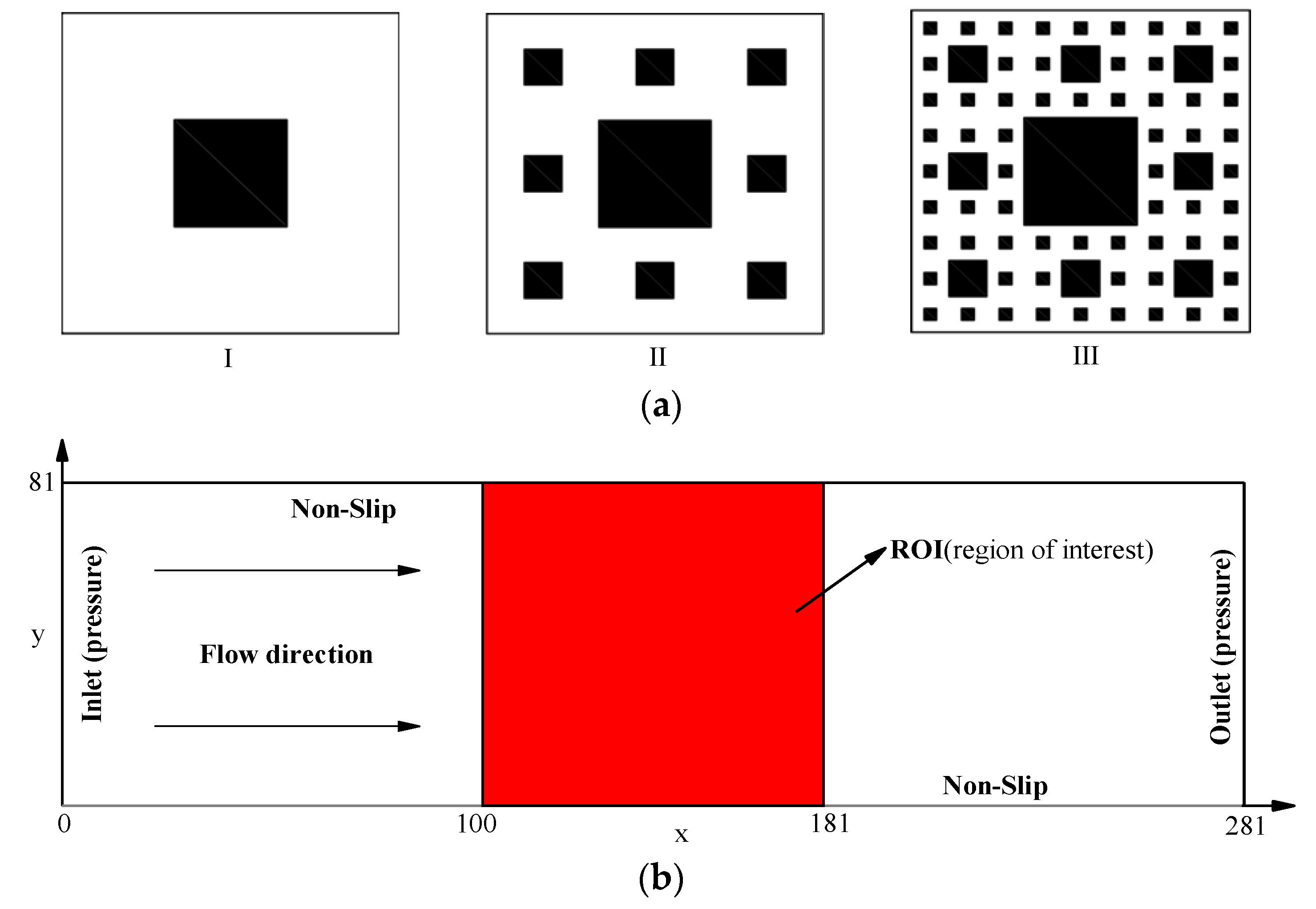
To achieve the goal of the study, a 2D dimensionless steady flow model is proposed as shown in Figure 1. The inlet and outlet are constant pressure boundaries, and pressure drop drives flow through region of interest (ROI). Sierpinski fractals with various structural complexities are utilized to construct geometry of porous media, as shown in Figure 1b. More obstacles (black) occupy the region, leading to evidently different pore (white) distribution and connectivity. Especially when ROI is none, the flow model becomes 2D Poiseuille flow, which can be used to verify the code for available theoretical solutions. When fractal patterns are in ROI, theoretical solution is not available, thus, numerical solution obtained by FEM is regarded as reference results to conduct the comparative study. Finally, the convergence criterion of all models is defined as [56]

$${\displaystyle \sum _i{\displaystyle \sum _j\frac{\sqrt{{\left({\mathsf{\nu }}_x\left(i,j,t+\delta t\right)-{\mathsf{\nu }}_x\left(i,j,t\right)\right)}^2+{\left({\mathsf{\nu }}_y\left(i,j,t+\delta t\right)-{\mathsf{\nu }}_y\left(i,j,t\right)\right)}^2}}{\sqrt{{\mathsf{\nu }}_x^2\left(i,j,t\right)+{\mathsf{\nu }}_y^2\left(i,j,t\right)+{10}^{-18}}}}}\le total\cdot err$$

(18)

where ${\mathsf{\nu }}_x\left(i,j,t\right)$, ${\mathsf{\nu }}_y\left(i,j,t\right)$, t and $t+\delta t$ are the x, y component velocity, present time and next time at lattice position (i, j), respectively. $total\cdot err$ in the paper is 10⁻⁷ and the criterion is stricter than previous work [56].

The physical properties and boundary conditions of flow model are listed in

Table 1. The physical properties and boundary condition of flow model.

Length of x	Length of y	Length of ROI	Width of ROI	Viscosity	Density	Inlet Pressure	Outlet Pressure
281	81	81	81	0.2	1.0	0.3667	0.3333

. The conversion between LBM units and actual physical units is avoided due to the dimensionless model. Reynolds number of LBM simulations is guaranteed to be the same with flow model, and modeling parameters and grid size are listed in

Table 2. The modeling parameters and grid size/grid resolution of LBM simulations.

Grid Size	281 × 81	562 × 162	843 × 243
Grid Resolution	1	2	3
Viscosity	0.2	0.4	0.6
τs	0.9091	0.5882	0.4348
τq	1.2308	1.5238	1.652
τρ= τd	1.0	1.0	1.0
τe = τε	0.8	0.8	0.8

. Generally, one specific fractal is simulated three times for each model with different grid size, or grid resolution, which is defined as the ration of grid size to physical size of flow model, and results lead to a more intuitive perspective of how grid resolution affects numerical accuracy.

3.2. Poiseuille Flow and Validation

2D Poiseuille flow, a laminar flow in parallel channels, is a common benchmark test for LBM simulation [20,56]. The comparison of theoretical solution and numerical results of all models is conducted to verify the reasonability of in-house code, and the results prove the validation of the code and can be used in further simulations.

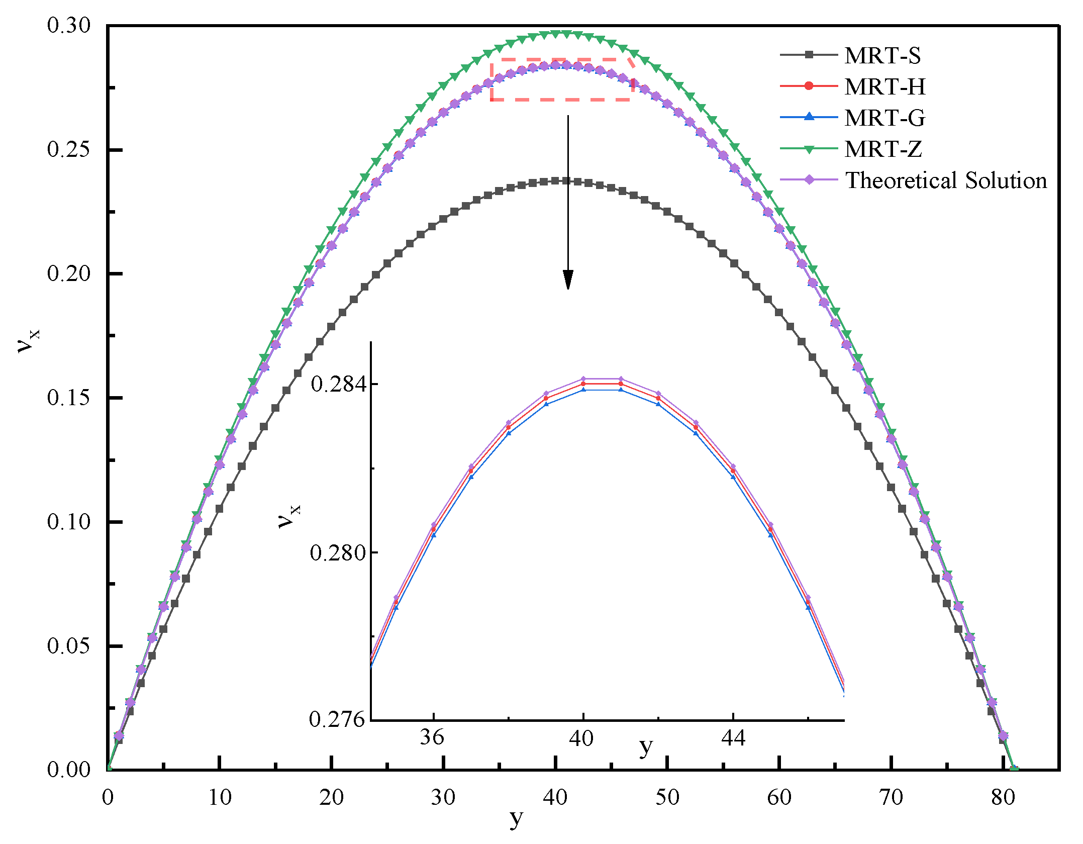
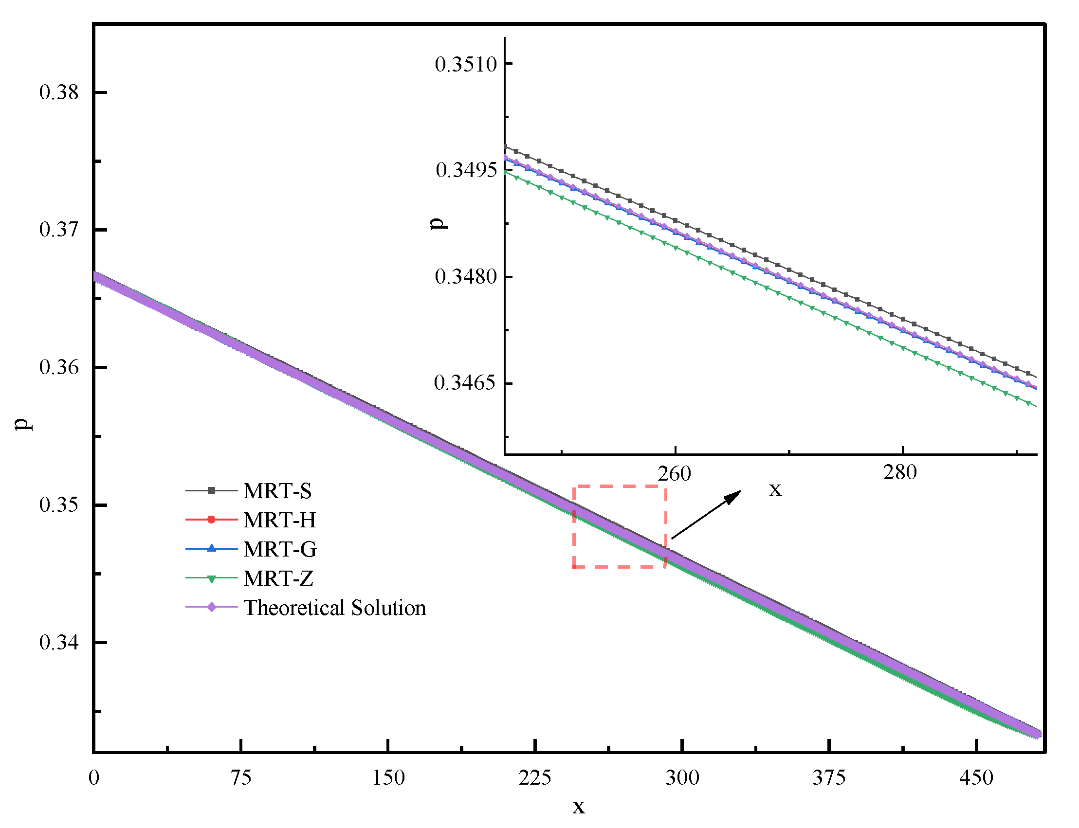
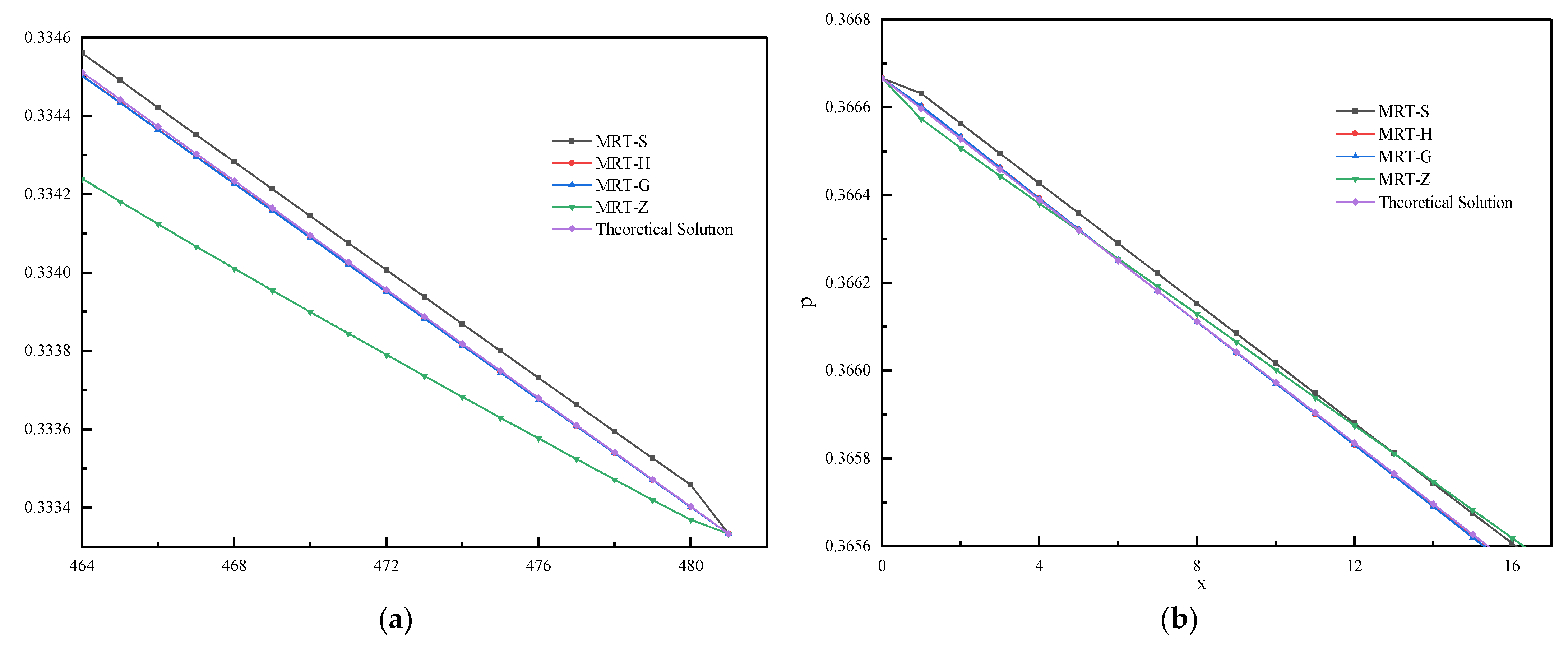
With Re = 115 (Reynolds number), the profiles of the x component of velocity $v_x$ along vertical centerlines of ROI (x = 140.5) are plotted in Figure 2. The results show He-Luo model and Guo’s model completely coincide with the theoretical solution, inversely the standard model is smaller and Zhang model is larger than the theoretical solution with both visible deviations. The pressure curve along channel centerline (y = 40.5) is shown in Figure 3, it seems like all models have a good agreement with theoretical solutions, however, if we zoom in on the local curve (green zone), it is obvious that He-Luo model and Guo’s model are more consistent with the theoretical solution, and clear deviations appear between the standard model and Zhang’s model. The deviations of Zhang’s model are quite strange, i.e., that the fluid pressure gradient is not a constant but varies in the line, which is different from the theoretical analysis. Therefore, the local curve near to the inlet and outlet is zoomed (Figure 4), visible deviations occur at the neighboring nodes of the in–out boundaries, and pressure is smaller in Zhang’s model while larger in the standard model, compared to our reference result. It is worth mentioning that the pressure curves of all models are parallel with the same slope in the middle, except Zhang’s model, whose curve intersects others and the slope changes, implying the worst performance on pressure. What makes the difference is that fluid pressure is the diagonal part of the second-order moments in Zhang’s model, but the zero order moment component in the other models.

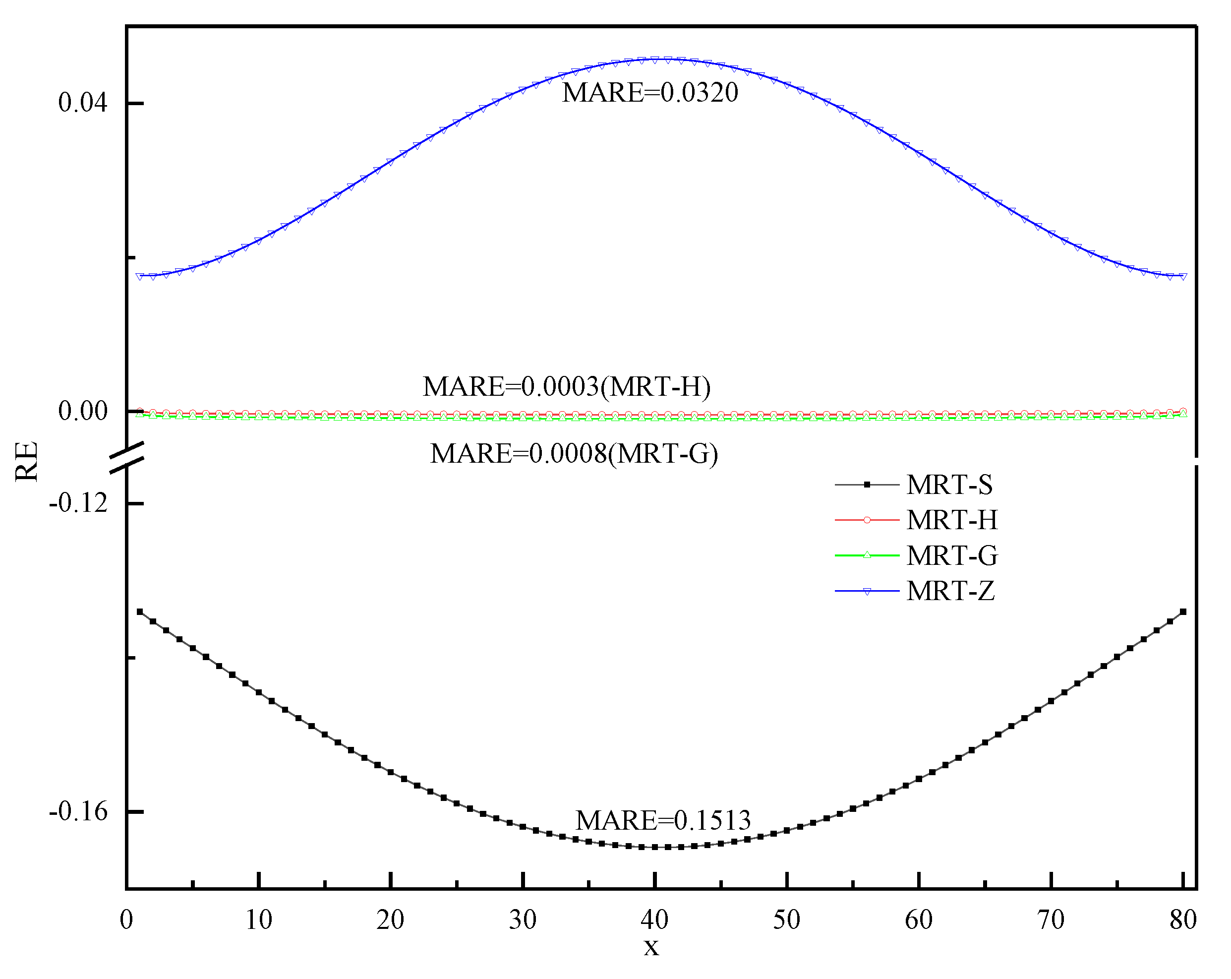
To further study numerical accuracy of models, the relative error (RE) and mean absolute relative error (MARE) of velocity are defined as

$$MARE=\frac{1}{N}{\displaystyle \sum _{i=1}^{N}R{E}_i}=\frac{1}{N}{\displaystyle \sum _N\frac{\left|res-ref\right|}{ref}}$$

(19)

where N is the number of compared points, res represents results of each model and ref is the FEM results or theoretical solutions (Poiseuille flow). MARE of x component velocity is focused for the velocity distribution attracting more attention in the non-linear flow regime, and ${\mathsf{\nu }}_y$ is too small and close to 0.

A conspicuous comparison about RE and MARE of ${\mathsf{\nu }}_x$ at x = 140.5 cross is shown in Figure 5. The REs of He-Luo model and Guo’s model are extremely small, leading to the MARE of 0.0003 and 0.0008, respectively. Inversely, the RE of standard model is the largest, with the largest MARE = 0.1513, and the RE of Zhang’s model is an order of magnitude smaller than standard model, with MARE = 0.0320. Moreover, different from He-Luo model and Guo’s model, the RE curves of standard model and Zhang’s model are parabolic profiles, which is the same as the velocity curves and implies the existence of compressible errors in both models because a larger velocity leads to a larger Ma. In general, the good improvements to the standard model are clearly reflected, RE of each model is tolerable and the results are quite accurate in all models. Therefore, the code is convincible to use in further investigation.

4. Results and Discussion

The LBM is indeed a similar simulation of the real problem with the same Reynolds number, thus, the geometric similarity scale, namely the grid size in the LBM, plays an important role. The dimensionless problem is designed and simulations with different grid resolutions (GRs) are performed in the paper. It is an established fact that high GR leads to high precision, but two questions are: Do different geometrical structures show the same rule about the effect of GR on numerical accuracy? How does structural complexity influence numerical accuracy? Both questions are discussed in greater depth later, according to the numerical results.

4.1. Grid Resolution

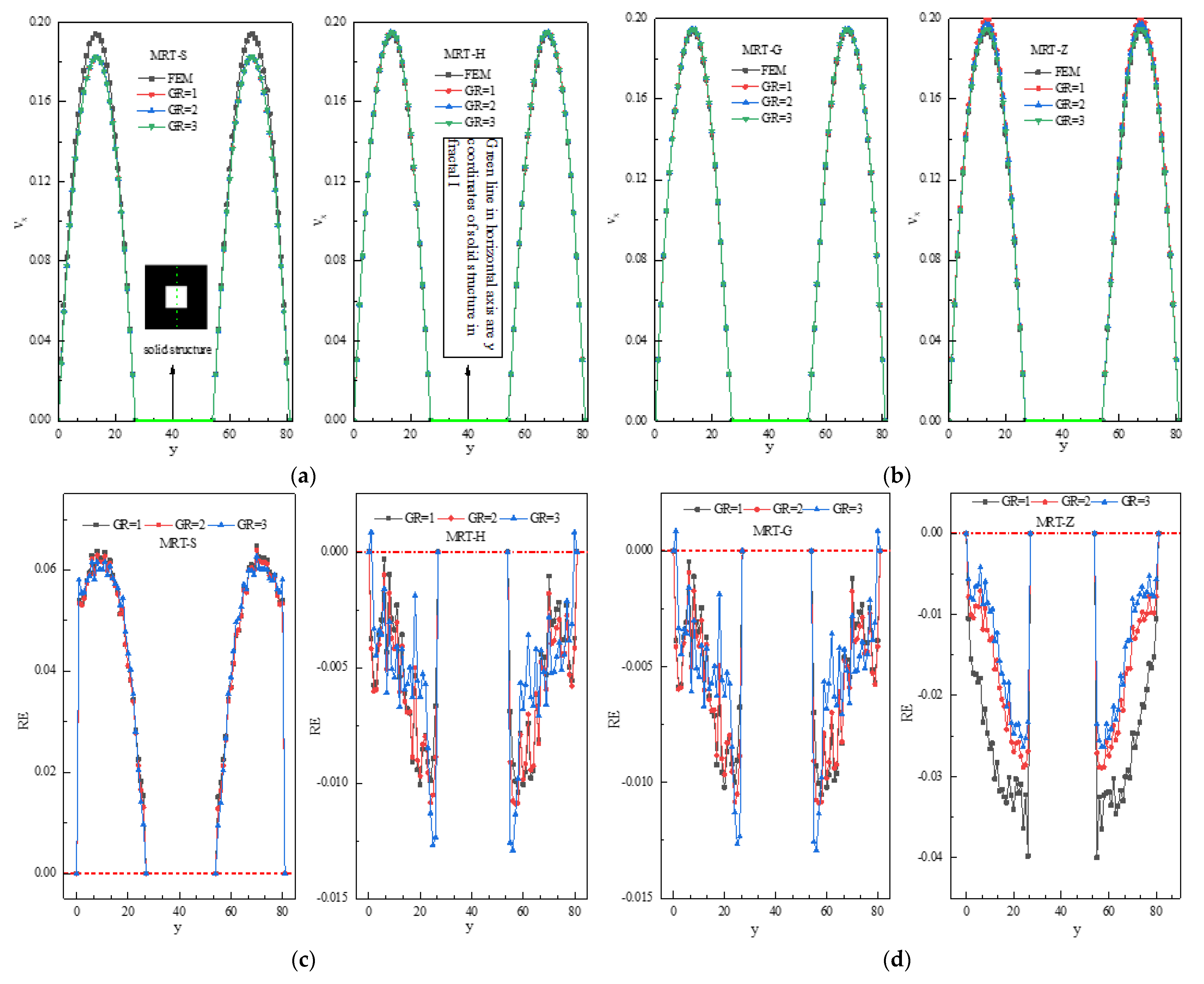
First, the relationship between accuracy and GR is investigated. Figure 6, Figure 7 and Figure 8 demonstrate the profiles and the RE of ${\mathsf{\nu }}_x$ along the vertical centerlines (x = 140.5) of the ROI with different geometries I, II and III, respectively. In structure I (Figure 6), the Reynolds number is 25, all velocity profiles of the LBM models are in good agreement with the reference results, except for the MRT-S model whose visible deviation from the reference is observed. The results really corroborate an established fact that the He-Luo, Guo’s and Zhang’s models perfect the compressible error of the LBE through the modification of the EDF. Figure 6c,d compare the RE curves of ${\mathsf{\nu }}_x$ with different GRs. The results show that the RE of Guo’s model and the He-Luo model are small and closed, the absolute value is less than 1.5% but with great fluctuation, while the relative error of the standard model and Zhang’s model are large with an absolute value of more than 6% and 4%, respectively, but with small fluctuations. Moreover, the RE of all models decreases as the GR increases, and Zhang’s model is particularly obvious.

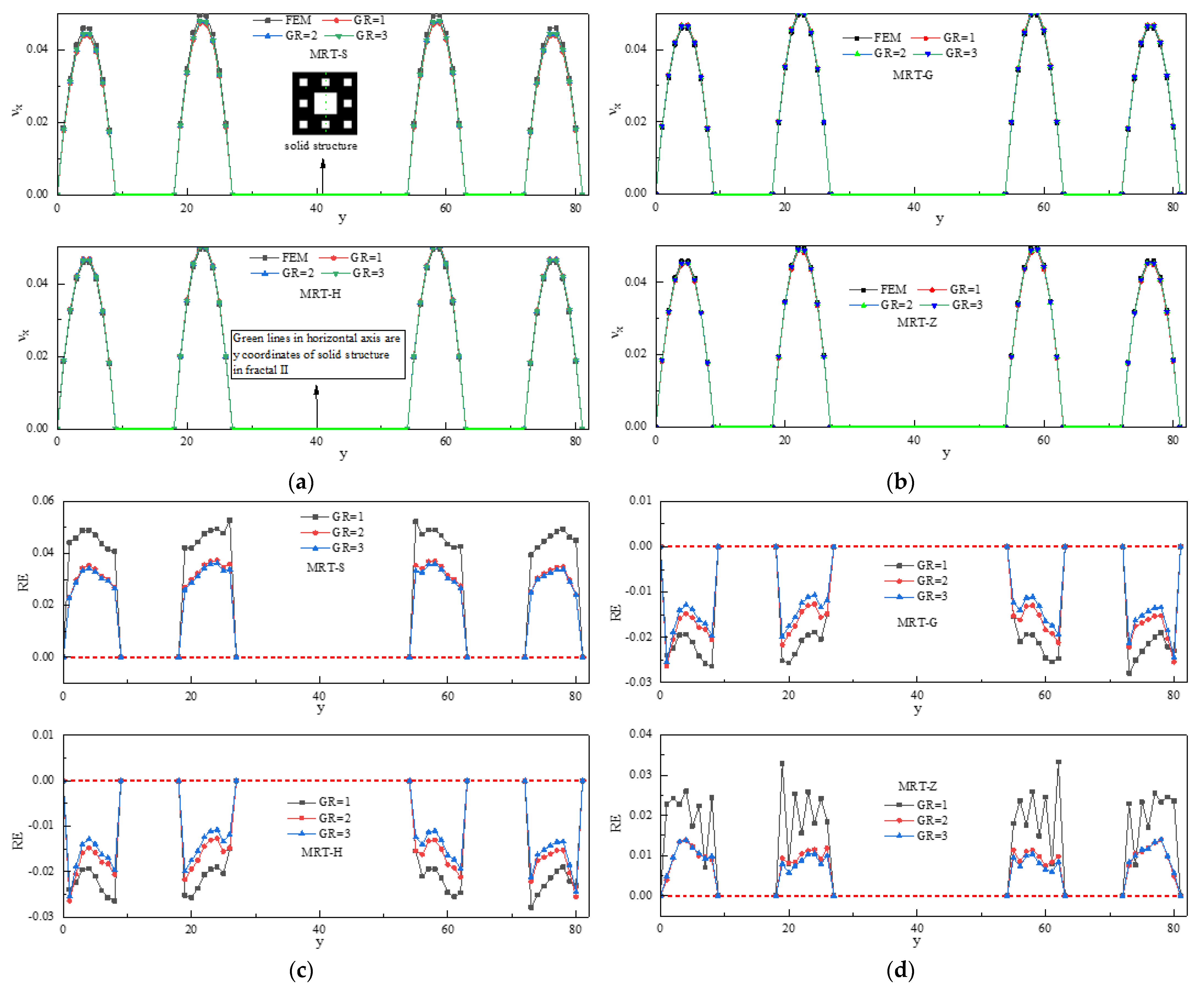
In structure II (Figure 7), the Reynolds number is 2, the disturbing deviations of the standard model are alleviated to some extent but are still visible, while the ${\mathsf{\nu }}_x$ curves of other models are consistent with the reference results. The RE curves of each model with different GRs are similar and approximately parallel to each other, i.e., the RE decreases as GR increases: a clearer relationship is plotted in Figure 7c,d. It is worth noting that when GR = 1, the ${\mathsf{\nu }}_x$ curve of Zhang’s model is approximately close to the reference result (Figure 7b), but the RE curve shows extremely strong volatility, namely the amplitude of variations obviously increases and the variations are violent and irregular (Figure 7d) when compared to the curves with GR = 2 and 3. Meanwhile, in the other models the RE curves have uniform curves no matter what the GR is. The observation implies that under the same conditions and convergence criterion, compared with other models, Zhang’s model has a poor computing stability, and the appearance of this occurred in previous work as well [38].

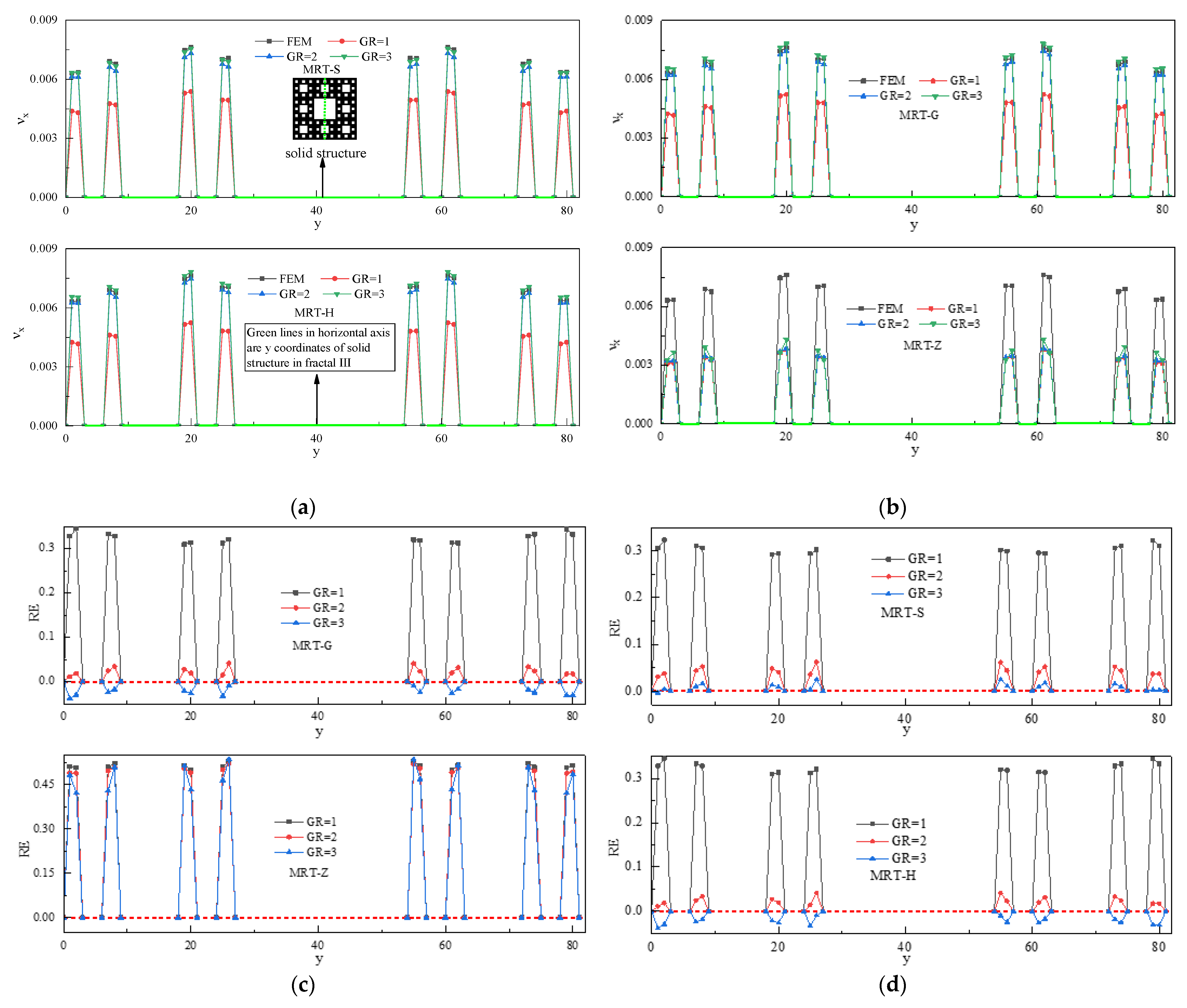
When the ROI is geometry III (Figure 8), the Reynolds number is 0.1, which also indicates that GR has a considerable effect on the accuracy of results: a higher GR leads to a smaller RE for all models. However, a worse problem about the validation of simulations is shown up. It is obvious to find; when the GR = 1, all models have an exaggeratedly large deviation from reference result, the RE exceeds 30%, and is even 50% for Zhang’s model, namely, the simulations under that scenario are quite inaccurate and invalid for all LBM models. However, when the GR becomes 2 and 3, the REs of the standard, He-Luo and Guo’ models are greatly reduced to within 5%, which is consistent with the reference result, but there is only a little decrease for Zhang’s model when the GR becomes bigger. It can be inferred Zhang’s model needs stricter requirements to acquire a better simulation compared to other models, especially with a complex domain. It is hard to regard the simulations as accurate and valid due to such exaggerated errors, although the results are indeed convergent. Computing stability improved by an MRT operator can efficiently improve computing stability, especially in a complex structure; even a divergent result with an SRT operator can become convergent by adopting an MRT operator, but the results may be very error prone if the GR is not high enough. Further inspections (such as flow balance) are necessary and are conducted in Section 4.3.

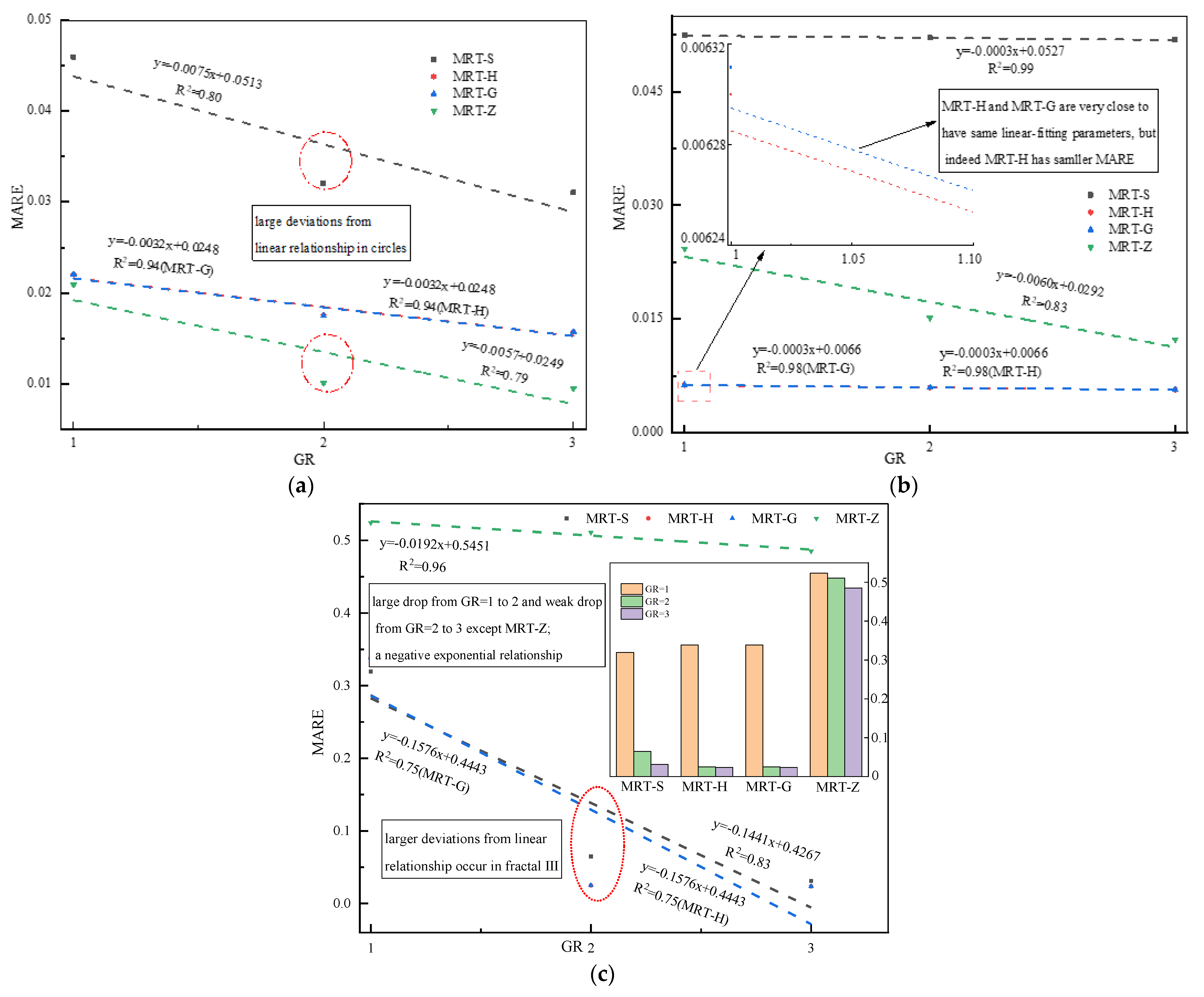
The curves of the MARE vary with GR and the linear-fitting curves are plotted to give a clear view (Figure 9). For the same geometry, all models show that the MARE decreases with the increase in GR, corresponding slope values are less than 0. The similar phenomenon appeared in Regulski’s work about the standard model [21]. Generally, a finer grid makes obstacles become better inscribed and uses more micro-particles to simulate macro variables, so the error is more localized and the flow simulation is more accurate globally.

4.2. Geometric Structure

The effect of the structural complexity on the accuracy of LBM simulations is seldom studied, and we first proposed the structural error to define the effect. Obviously, fractals I, II and III have different structural complexities to some extent. However, no matter how complex the structure is, the structural boundaries are marked as solid nodes and implemented by a half-way bounce-back scheme in the LBM. In other words, the intuitive performances of structural complexity are the number of BCs and minimum grid distance of different obstacles. In geometry I, II and III, the minimum grid distance of obstacles is 27, 9 and 3, respectively, and the number of BCs is 4, 8 and 16, including top and bottom walls, respectively. The proportion of BC points (${\mathsf{\nu }}_x=0$) grows larger when the structure becomes more complex, even up to 50% in geometry III. Therefore, to correctly reflect structural error, only fluid nodes are contained to calculate the MARE (all solid nodes are non-slip with zero velocity).

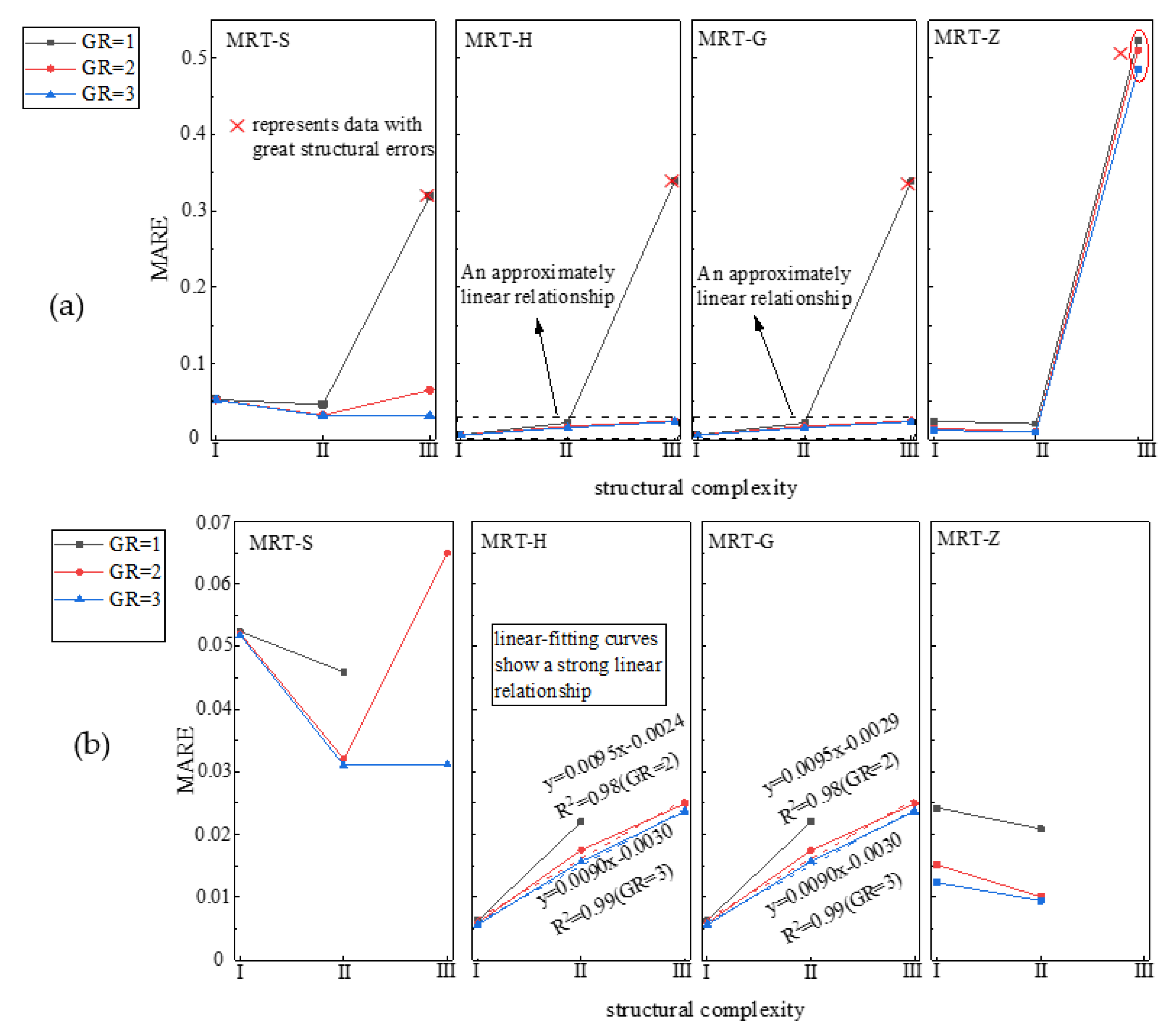
Figure 10a shows that the MARE curves of each model vary with different geometric structures. No obvious or intuitive regulation can be found, except for the data in the red box for He-Luo and Guo’s model, showing a visible linear relationship. Apparently, the data points with an overlarge MARE seriously affect the presentation of the results and rule, such as the MARE of geometry III for all models exceeds 30% with GR = 1, and they all exceed 45% in Zhang’s model regardless of the GRs, implying that the simulations are not convincible; the details are explained in Section 4.3. After removing the unreasonable data points, the clearer curves are plotted in Figure 10b. Obviously, there is an approximately linear relationship between the MARE and structural complexity in the He-Luo and Guo’s model, but the rule is not the same for the standard and Zhang’s model, due to the compressible effect. In fact, all models have a compressible error, but it is regarded as a high-order small error and ignored in the CE analysis for the He-Luo model, Guo’s model and Zhang’s model, although the compressible error cannot be completely ignored in Zhang’s model as discussed above. Therefore, the MARE represents the total error, including two parts: the compressible error and structural error. The characteristic velocity (maximum speed) quickly reduces from 0.1942 in fractal I to 0.0076 in fractal III (Figure 6, Figure 7 and Figure 8), leading to Ma and the compressible error dramatically descends, but the structure becomes more complex as well causing structural error increase. In the He-Luo model and Guo’s model, structural error is dominant in the MARE due to the ignored compressible error, thus, the MARE increases with structural complexity; however, the compressible error and structural error in the standard model and Zhang’s model are both considerable, and the combined effects show a descending–increasing process.

Structural error significantly decreases with increasing GRs for a better inscription of the geometrical structure. The RE and MARE discussed above are for total error without distinguishing the structural error, and it can be inferred that the same fractal has the same compressible error due to the same characteristic velocity and Ma, namely, structural error is the decisive factor in RE curves. If we consider Figure 9 again, the He-Luo model and Guo’s model are very closed and even have the same fitted parameters, but the former has a smaller MRAE. When the ROI moves from fractal I to III, the absolute slope of the fitted curves is 0.0003, 0.0032 and 0.1576, respectively, indicating that the GR is more obvious for improving numerical accuracy in complex structures. Large deviations from linear curves are visible in geometry III, and the histogram further shows a negative exponential relationship in geometry II and III (Figure 9). The standard model shows a linear relationship in geometry I, but a negative exponential relationship in other fractals. Figure 11 shows that negative exponential fitting curves perform better than linear curves in Figure 9, and the R (fitting index) almost always increases. Apparently, structural error descends with GR and shows an approximately negative exponential relationship, especially when the structure is complex and the GR is not high enough. In fractal I, GR = 1 is enough to simulate and show a flat part of the exponential curve, just approximately kept linear.

4.3. Flow Balance and Efficiency

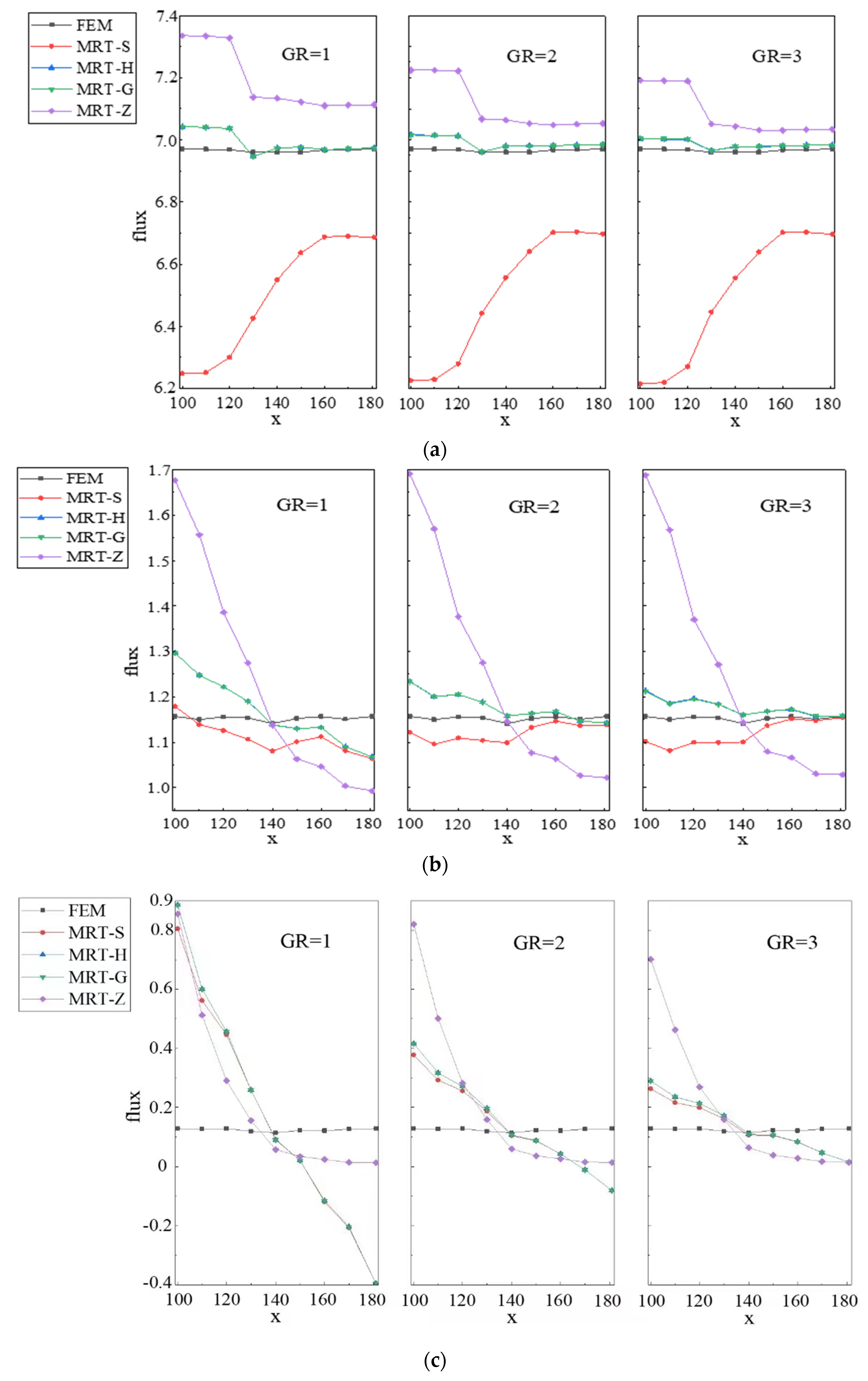
The above results and discussion all focus on the velocity profile and relative error at the x = 140.5 vertical centerline of the ROI, and a complete understanding of the global simulation is lacking. Therefore, the flow balance inspection and computing efficiency are investigated in this section. The conservation of mass in the ROI is reflected by flux curves, which are in fact a continuum equation. Figure 12 shows flux curves along the x direction under various predetermined conditions.

In geometry I, flux curves of the standard model are always lower than the reference result, while other models are larger, and all models gradually approach the reference result. In geometry II, flux curves of the standard model, He-Luo model and Guo’s model gradually flatten with increasing GRs and get closer to the reference curve, and the flux difference between the inlet and outlet also decreases, all of which imply a better simulation and accuracy. However, the flow curves of Zhang’s model are quite strange: the inlet and outlet flux are 1.4 times and 0.9 times of the reference value, respectively, leading to a huge differential flux. In addition, flow curves are just like a negative exponential profile, seriously violating the mass conservation equation. In geometry III, flow curves of all models produce a huge differential flux for serious structural error when GR = 1, even the outlet flux is less than 0, which is impossible. However, the standard model, He-Luo model and Guo’s model sharply flatten with a significantly decreased differential flux when the GR becomes 2 and 3, indicating that better global flow simulations are obtained by increasing the GR. Inversely, flux curves are seldom closer to the reference results with a slightly reduced differential flux, the global flow is still terrible in Zhang’s model. There is no doubt that results of all models in fractal III with GR = 1 and Zhang’s model in fractal II and III are unreasonable and invalid because the GR is so small that there are not enough micro-particles to simulate the macro flow in the complex structure, and this leads to an incredible relative error. If we just imagine Poiseuille flow with a channel width = 3, it is impossible to obtain accurate results by using the D2Q9 model with GR = 1 because the micro-particles are too sparse to simulate the macro flow; this violates kinetic theory, namely using quantities of micro-particles to simulate the macro flow. However, it must be emphasized that the unreasonable results do not indicate that Zhang’s model is problematic, but they imply that Zhang’s model needs a larger GR to obtain the same simulations compared with other models.

Computational efficiency is another key index to determine the superiority of models. The number of iterations of all simulations are listed in

Table 3. Number of iterations necessary for convergence criterion.

	281 × 81				562 × 162				843 × 243
	MRT-S	MRT-H	MRT-G	MRT-Z	MRT-S	MRT-H	MRT-G	MRT-Z	MRT-S	MRT-H	MRT-G	MRT-Z
I	16,168	21,395	20,792	14,584	34,613	40,178	38,268	21,292	44,250	54,450	50,544	32,749
II	11,249	12,740	12,596	7395	31,938	29,092	24,638	14,696	34,240	40,168	38,125	18,764
II	12,068	12,144	11,242	9275	16,765	22,794	20,959	13,252	36,541	37,805	35,254	21,600

. Only the EDF and macroscopic variables calculation are different, thus, each step can be regarded as equally time-consuming for similar processes in each model. Therefore, the number of iterations necessary for convergence criterion can persuasively indicate the efficiency of each model. In order to make efficiency measurements more credible, it is worth mentioning that all models were coded in the same language, by the same person and run on the same computer.

In general, in a specific fractal with the same GR, the number of iterations approximately satisfies: MRT-H > MRT-G (MRT-S) > MRT-Z, indicating that Zhang’s model has the highest computational efficiency and the fastest convergence rate; however, the other three models are more stable. With the same convergence criterion, Zhang’s model performs worse in accuracy and stability of the simulation, which is also confirmed in previous research [38]. In this paper, some results of Zhang’s model are unreasonable, and it is likely that the convergence criterion are too loose and the GR is not high enough. To obtain the same accuracy with other models, stricter settings for GR and $total\cdot err$ are needed. Another interesting finding is that the number of iterations decreases as the geometrical structure becomes more complex. From fractal I to Ⅲ, the number of iterations to reach convergence reduces in each model. A more complex structure means more BCs and a smaller grid distance between obstacles, leading to the influent and spread area of pressure boundary and peak velocity becoming smaller, so it is easier and needs fewer iterations to reach an equilibrium state in a local simulation.

5. Conclusions

The different LBM models for incompressible flow with an MRT collision operator are investigated in terms of their numerical performance. Generally, in contrast to the standard model, the He-Luo model, Guo’s model and Zhang’s model do indeed weaken compressible error and improve numerical accuracy. However, the effect of compressibility can be ignored in the He-Luo model and Guo’s model, while compressible error cannot be completely ignored in Zhang’s model as expected.

As well as the compressible error of LBM models, geometrical structure also influences the numerical accuracy, and the effect of structure is first investigated and defined as structural error in this paper. In the He-Luo model and Guo’s model, the compressible error is negligible and structural error is primary, but both should be considered in Zhang’s model and the standard model. In a specific structure, the compressible error is constant in theory because of the same Ma and velocity profiles no matter what the GR is, but structural error obviously decreases with increasing GR and shows an approximately negative exponential relationship. Commonly, a more complex structure requires a higher grid resolution to inscribe, and more micro-particles to simulate, otherwise a lower grid resolution can lead to exaggerated structural errors and even wrong results. Structural error is determined by structural complexity with an approximately linear relationship in the paper. With the same GR, a more complex structure is implemented by more bounce-back scheme boundaries and produces more local errors, leading to a larger global structural error. However, different models have different sensitivity (or requirement) to grid resolution, which strongly reflects the robust and computing stability of models. Compared with other models, Zhang’s model needs a stricter grid resolution and convergence criterion to obtain a better simulation, implying flaws in the computing stability.

The computing efficiency of models is investigated according to the number of iterations. Zhang’s model has the fastest convergence rate, while convergence rates of the He-Luo mode and Guo’ model are slow, but the results are more accurate. Moreover, a complex structure leads to a smaller domain affected by boundary condition, thus, it is easier to reach a local equilibrium state and requires less iterations to reach convergence for all models, which is counterintuitive and contrary to traditional CFD but further proves the superiority of LBM application in a micro-flow simulation.

Generally, the standard model is seriously affected by compressible error, leading to the largest error in all simulations. The He-Luo model and Guo’s model do indeed eliminate the compressible error and have a good performance in accuracy, although both convergence rates are slower. Zhang’s model has an advantage in its convergence rate but with terrible computational stability and considerable compressible error, and needs a stricter convergence criterion and grid resolution. Therefore, after comprehensively considering its numerical accuracy and the fact it is time-consuming, Guo’s model is strongly recommended to simulate a micro steady flow in a complex geometrical structure.

References

- Inamuro, T.; Yoshino, M.; Ogino, F. Accuracy of the lattice Boltzmann method for small Knudsen number with finite Reynolds number. Phys. Fluids 1997, 9, 3535–3542. [Google Scholar] [CrossRef]
- Farahani, M.V.; Foroughi, S.; Norouzi, S.; Jamshidi, S. Mechanistic Study of Fines Migration in Porous Media Using Lattice Boltzmann Method Coupled with Rigid Body Physics Engine. J. Energy Resour. Technol. 2019, 141, 123001. [Google Scholar] [CrossRef]
- Keshtkar, M.M. Numerical simulation of fluid flow in random granular porous media using lattice Boltzmann method. Int. J. Adv. Des. Manuf. Technol. 2016, 9, 31–40. [Google Scholar]
- Zarei, A.; Karimipour, A.; Isfahani, A.H.M.; Tian, Z. Improve the performance of lattice Boltzmann method for a porous nanoscale transient flow by provide a new modified relaxation time equation. Phys. A Stat. Mech. Appl. 2019, 535. [Google Scholar] [CrossRef]
- Deen, N.G.; Annaland, M.V.S.; Kuipers, J.A.M. Detailed computational and experimental fluid dynamics of fluidized beds. Appl. Math. Model. 2006, 30, 1459–1471. [Google Scholar] [CrossRef] [Green Version]
- Ryu, S.; Ko, S. A comparative study of lattice boltzmann and volume of fluid method for two-dimensional multiphase flows. Nucl. Eng. Technol. 2012, 44, 623–638. [Google Scholar] [CrossRef] [Green Version]
- Xie, C.; Zhang, J.; Wang, M. Lattice Boltzmann Modeling of Non-Newtonian Multiphase Fluid Displacement. Chin. J. Comput. Phys. 2016, 33, 147–155. [Google Scholar]
- Zhou, P.; Guo, D.; Kang, R.; Jin, Z. Analysis of Laminar Flow Over a Non-Conventional Random Rough Surface Based on Lattice Boltzmann Method. J. Tribol. 2012, 134, 012201. [Google Scholar] [CrossRef]
- Paradis, H.; Andersson, M.; Sunden, B. Modeling of mass and charge transport in a solid oxide fuel cell anode structure by a 3D lattice Boltzmann approach. Heat Mass Transf. 2016, 52, 1529–1540. [Google Scholar] [CrossRef]
- Yan, W.; Wu, J.; Yang, S.; Wang, Y. Numerical investigation on characteristic flow regions for three staggered stationary circular cylinders. Eur. J. Mech. B-Fluids 2016, 60, 48–61. [Google Scholar] [CrossRef]
- Chalons, C.; Fox, R.O.; Laurent, F.; Massot, M.; Vie, A. Multivariate Gaussian Extended Quadrature Method of Moments for Turbulent Disperse Multiphase Flow. Multiscale Model. Simul. 2017, 15, 1553–1583. [Google Scholar] [CrossRef] [Green Version]
- Peng, C.; Ayala, O.M.; de Motta, J.C.B.; Wang, L.-P. A comparative study of immersed boundary method and interpolated bounce-back scheme for no-slip boundary treatment in the lattice Boltzmann method: Part II, turbulent flows. Comput. Fluids 2019, 192. [Google Scholar] [CrossRef] [Green Version]
- Basagaoglu, H.; Harwell, J.R.; Hoa, N.; Succi, S. Enhanced computational performance of the lattice Boltzmann model for simulating micron- and submicron-size particle flows and non-Newtonian fluid flows. Comput. Phys. Commun. 2017, 213, 64–71. [Google Scholar] [CrossRef]
- Delouei, A.A.; Nazari, M.; Kayhani, M.H.; Kang, S.K.; Succi, S. Non-Newtonian particulate flow simulation: A direct-forcing immersed boundary-lattice Boltzmann approach. Phys. A Stat. Mech. Appl. 2016, 447, 1–20. [Google Scholar] [CrossRef]
- Tarksalooyeh, V.W.A.; Zavodszky, G.; van Rooij, B.J.M.; Hoekstra, A.G. Inflow and outflow boundary conditions for 2D suspension simulations with the immersed boundary lattice Boltzmann method. Comput. Fluids 2018, 172, 312–317. [Google Scholar] [CrossRef]
- Banda, M.K.; Junk, M.; Klar, A. Kinetic derivation of a finite difference scheme for the incompressible Navier-Stokes equation. J. Comput. Appl. Math. 2003, 154, 341–354. [Google Scholar] [CrossRef] [Green Version]
- Junk, M.; Yong, W.A. Rigorous Navier-Stokes limit of the lattice Boltzmann equation. Asymptot. Anal. 2003, 35, 165–185. [Google Scholar]
- Pan, C.; Luo, L.-S.; Miller, C.T. An evaluation of lattice Boltzmann schemes for porous medium flow simulation. Comput. Fluids 2006, 35, 898–909. [Google Scholar] [CrossRef]
- Hazi, G. Accuracy of the lattice Boltzmann method based on analytical solutions. Phys. Rev. E 2003, 67, 056705. [Google Scholar] [CrossRef] [Green Version]
- Guo, Z.; Liu, H.; Luo, L.-S.; Xu, K. A comparative study of the LBE and GKS methods for 2D near incompressible laminar flows. J. Comput. Phys. 2008, 227, 4955–4976. [Google Scholar] [CrossRef]
- Regulski, W.; Szumbarski, J. Numerical simulation of confined flows past obstacles—The comparative study of Lattice Boltzmann and Spectral Element Methods. Arch. Mech. 2012, 64, 423–456. [Google Scholar]
- Zhao, Y.; Zhu, G.; Zhang, C.; Liu, S.; Elsworth, D.; Zhang, T. Pore-Scale Reconstruction and Simulation of Non-Darcy Flow in Synthetic Porous Rocks. J. Geophys. Res. Solid Earth 2018, 123, 2770–2786. [Google Scholar] [CrossRef]
- Muljadi, B.P.; Blunt, M.J.; Raeini, A.Q.; Bijeljic, B. The impact of porous media heterogeneity on non-Darcy flow behaviour from pore-scale simulation. Adv. Water Resour. 2016, 95, 329–340. [Google Scholar] [CrossRef]
- Blunt, M.J.; Bijeljic, B.; Dong, H.; Gharbi, O.; Iglauer, S.; Mostaghimi, P.; Paluszny, A.; Pentland, C. Pore-scale imaging and modelling. Adv. Water Resour. 2013, 51, 197–216. [Google Scholar] [CrossRef] [Green Version]
- Golparvar, A.; Zhou, Y.; Wu, K.; Ma, J.; Yu, Z. A comprehensive review of pore scale modeling methodologies for multiphase flow in porous media. Adv. Geo-Energy Res. 2018, 2, 418–440. [Google Scholar] [CrossRef] [Green Version]
- Song, Y.; Davy, C.A.; Thang Nguyen, K.; Troadec, D.; Hauss, G.; Jeannin, L.; Adler, P.M. Two-scale analysis of a tight gas sandstone. Phys. Rev. E 2016, 94, 043316. [Google Scholar] [CrossRef] [PubMed]
- Song, R.; Wang, Y.; Liu, J.; Cui, M.; Lei, Y. Comparative analysis on pore-scale permeability prediction on micro-CT images of rock using numerical and empirical approaches. Energy Sci. Eng. 2019, 7, 2842–2854. [Google Scholar] [CrossRef]
- Li, J.; Ho, M.T.; Wu, L.; Zhang, Y. On the unintentional rarefaction effect in LBM modeling of intrinsic permeability. Adv. Geo-Energy Res. 2018, 2, 404–409. [Google Scholar] [CrossRef]
- Zou, Q.S.; Hou, S.L.; Chen, S.Y.; Doolen, G.D. An improved incompressible lattice boltzmann model for time-independent flows. J. Stat. Phys. 1995, 81, 35–48. [Google Scholar] [CrossRef]
- He, X.Y.; Luo, L.S. Lattice Boltzmann model for the incompressible Navier-Stokes equation. J. Stat. Phys. 1997, 88, 927–944. [Google Scholar] [CrossRef]
- Bhatnagar, P.L.; Gross, E.P.; Krook, M. A model for collision processes in gases.1. small amplitude processes in charged and neutral one-component systems. Phys. Rev. 1954, 94, 511–525. [Google Scholar] [CrossRef]
- Lin, Z.F.; Fang, H.P.; Tao, R.B. Improved lattice Boltzmann model for incompressible two-dimensional steady flows. Phys. Rev. E 1996, 54, 6323–6330. [Google Scholar] [CrossRef]
- Qian, Y.H.; Dhumieres, D.; Lallemand, P. Lattice BGK models for navier-stokes equation. Europhys. Lett. 1992, 17, 479–484. [Google Scholar] [CrossRef]
- An, S.; Yu, H.; Wang, Z.; Kapadia, B.; Yao, J. Unified mesoscopic modeling and GPU-accelerated computational method for image-based pore-scale porous media flows. Int. J. Heat Mass Transf. 2017, 115, 1192–1202. [Google Scholar] [CrossRef]
- Reider, M.B.; Sterling, J.D. Accuracy of discrete-velocity bgk models for the simulation of the incompressible navier-stokes equations. Comput. Fluids 1995, 24, 459–467. [Google Scholar] [CrossRef] [Green Version]
- He, X.Y.; Zou, Q.S.; Luo, L.S.; Dembo, M. Analytic solutions of simple flows and analysis of nonslip boundary conditions for the lattice Boltzmann BGK model. J. Stat. Phys. 1997, 87, 115–136. [Google Scholar] [CrossRef]
- Guo, Z.L.; Shi, B.C.; Wang, N.C. Lattice BGK model for incompressible Navier-Stokes equation. J. Comput. Phys. 2000, 165, 288–306. [Google Scholar] [CrossRef]
- Zhang, L.; Zeng, Z.; Xie, H.; Zhang, Y.; Lu, Y.; Yoshikawa, A.; Mizuseki, H.; Kawazoe, Y. A comparative study of lattice Boltzmann models for incompressible flow. Comput. Math. Appl. 2014, 68, 1446–1466. [Google Scholar] [CrossRef]
- Grad, H. Note on n-dimensional hermite polynomials. Commun. Pure Appl. Math. 1949, 2, 325–330. [Google Scholar] [CrossRef]
- Dellar, P.J. Nonhydrodynamic modes and a priori construction of shallow water lattice Boltzmann equations. Phys. Rev. E 2002, 65. [Google Scholar] [CrossRef] [Green Version]
- Newman, M.S.; Yin, X. Lattice Boltzmann Simulation of Non-Darcy Flow In Stochastically Generated 2D Porous Media Geometries. SPE J. 2013, 18, 12–26. [Google Scholar] [CrossRef]
- Cousins, T.A.; Ghanbarian, B.; Daigle, H. Three-Dimensional Lattice Boltzmann Simulations of Single-Phase Permeability in Random Fractal Porous Media with Rough Pore-Solid Interface. Transp. Porous Med. 2018, 122, 527–546. [Google Scholar] [CrossRef]
- Zhang, G.; Zhang, Y.; Xu, A.; Li, Y. Microflow effects on the hydraulic aperture of single rough fractures. Adv. Geo-Energy Res. 2019, 3, 104–114. [Google Scholar] [CrossRef]
- Grucelski, A.; Pozorski, J. Lattice Boltzmann simulations of flow past a circular cylinder and in simple porous media. Comput. Fluids 2013, 71, 406–416. [Google Scholar] [CrossRef]
- Fu, J.; Dong, J.; Wang, Y.; Ju, Y.; Owen, D.R.J.; Li, C. Resolution Effect: An Error Correction Model for Intrinsic Permeability of Porous Media Estimated from Lattice Boltzmann Method. Transp. Porous Med. 2020, 132, 627–656. [Google Scholar] [CrossRef]
- Zou, Q.S.; He, X.Y. On pressure and velocity boundary conditions for the lattice Boltzmann BGK model. Phys. Fluids 1997, 9, 1591–1598. [Google Scholar] [CrossRef] [Green Version]
- Maier, R.S.; Bernard, R.S.; Grunau, D.W. Boundary conditions for the lattice Boltzmann method. Phys. Fluids 1996, 8, 1788–1801. [Google Scholar] [CrossRef]
- Lee, Y.-H.; Huang, L.-M.; Zou, Y.-S.; Huang, S.-C.; Lin, C.-A. Simulations of turbulent duct flow with lattice Boltzmann method on GPU cluster. Comput. Fluids 2018, 168, 14–20. [Google Scholar] [CrossRef]
- Prestininzi, P.; La Rocca, M.; Hinkelmann, R. Comparative Study of a Boltzmann-based Finite Volume and a Lattice Boltzmann Model for Shallow Water Flows in Complex Domains. Int. J. Offshore Polar Eng. 2014, 24, 161–167. [Google Scholar]
- Luo, L.-S.; Liao, W.; Chen, X.; Peng, Y.; Zhang, W. Numerics of the lattice Boltzmann method: Effects of collision models on the lattice Boltzmann simulations. Phys. Rev. E 2011, 83, 056710. [Google Scholar] [CrossRef] [Green Version]
- Tao, S.; Hu, J.; Guo, Z. An investigation on momentum exchange methods and refilling algorithms for lattice Boltzmann simulation of particulate flows. Comput. Fluids 2016, 133, 1–14. [Google Scholar] [CrossRef]
- Wang, H.; Yuan, X.; Liang, H.; Chai, Z.; Shi, B. A brief review of the phase-field-based lattice Boltzmann method for multiphase flows. Capillarity 2019, 2, 33–52. [Google Scholar] [CrossRef] [Green Version]
- Guo, Z.; Zheng, C.; Shi, B. An extrapolation method for boundary conditions in lattice Boltzmann method. Phys. Fluids 2002, 14, 2007–2010. [Google Scholar] [CrossRef]
- Chen, L.; Yu, Y.; Lu, J.; Hou, G. A comparative study of lattice Boltzmann methods using bounce-back schemes and immersed boundary ones for flow acoustic problems. Int. J. Numer. Methods Fluids 2014, 74, 439–467. [Google Scholar] [CrossRef]
- Peng, C.; Ayala, O.M.; Wang, L.-P. A comparative study of immersed boundary method and interpolated bounce-back scheme for no-slip boundary treatment in the lattice Boltzmann method: Part I., laminar flows. Comput. Fluids 2019, 192, 104233. [Google Scholar] [CrossRef] [Green Version]
- Hu, K.; Meng, J.; Zhang, H.; Gu, X.-J.; Emerson, D.R.; Zhang, Y. A comparative study of boundary conditions for lattice Boltzmann simulations of high Reynolds number flows. Comput. Fluids 2017, 156, 1–8. [Google Scholar] [CrossRef]
Figure 1.
(a) The structure of ROI (white pore and black obstacles). (b) The diagram of flow model.
Figure 2.
The profiles of along vertical centerline of ROI (x = 140.5).
Figure 3.
The profiles of pressure along channel centerline (y = 40.5).
Figure 4.
(a)The profiles of pressure at inlet boundary; (b) The profiles of pressure at outlet boundary.
Figure 5.
RE and MARE of along vertical centerline of ROI (x = 140.5).
Figure 6.
(a,b) The profiles of along vertical centerline of ROI (x = 140.5) in fractal I. (c,d) RE curves of along vertical centerline of ROI (x = 140.5) in fractal I.
Figure 7.
(a,b) The profiles of along vertical centerline of ROI (x = 140.5) in fractal II. (c,d) RE curves of along vertical centerline of ROI (x = 140.5) in fractal II.
Figure 8.
(a,b) The profiles of along vertical centerline of ROI (x = 140.5) in fractal III; (c,d) RE curves of along vertical centerline of ROI (x = 140.5) in fractal III.
Figure 9.
(a) MARE vary with different GRs in fractal I. (b) MARE vary with different GRs in fractal II; (c) MARE vary with different GRs in fractal III.
Figure 10.
(a) MARE curves vary with different fractal structures; (b) MARE curves vary with different fractal structures after removing unreasonable points with great structural errors.
Figure 11.
MARE curves of different fractal structures vary with GRs in negative exponential form.
Figure 12.
(a) Flux curves of fractal I. (b) Flux curves of fractal II. (c) Flux curves of fractal III.