Time-Domain Circuit Modelling for Hybrid Supercapacitors

Abstract

Classic circuit modeling for supercapacitors is limited in representing the strongly non-linear behavior of the hybrid supercapacitor technology. In this work, two novel modeling techniques suitable to represent the time-domain electrical behavior of a hybrid supercapacitor are presented. The first technique enhances a well-affirmed circuit model by introducing specific non-linearities. The second technique models the device through a black-box approach with a neural network. Both the modeling techniques are validated experimentally using a workbench to acquire data from a real hybrid supercapacitor. The proposed models, suitable for different supercapacitor technologies, achieve higher accuracy and generalization capabilities compared to those already presented in the literature. Both modeling techniques allow for an accurate representation of both short-time domain and steady-state simulations, providing a valuable asset in electrical designs featuring supercapacitors.

1. Introduction

Supercapacitors (SC) are widely adopted as Energy Storage Systems (ESS) in several applications, because of properties such as suitability for fast and efficient charging, high-power density, and low internal resistance. One more advantage of the SCs is that they have a reduced recharge time if compared to Li-ion batteries; commercially available SCs do not typically rely on redox reactions at the electrodes, so that a limited resistance is opposed towards energy storing and release [1]. Additionally, in practical applications, the time required to store a specified energy amount at nominal levels of charge is at least 50% shorter than that required by batteries. Moreover, SCs result in a long life and wide operative temperature range, thus, SCs are a promising alternative to traditional batteries and lead to the so-called Hybrid Energy Storage Systems (HESS) [2].

To properly size an SC pack, an equivalent model reproducing the dynamic behavior of each cell is crucial. An appropriate dynamic behavior model must reproduce both the transient and the steady-state response of an SC. That is, the model must accurately reproduce the voltage/current dynamic characteristic and must correctly predict the power loss occurring during the charge and discharge process [3].

Although very complex models could be implemented, simplicity is often a desirable characteristic. This is for three main reasons: (a) computational, since the model is often a part of a time-domain or frequency-domain simulation of a switched-type circuit (e.g., a DC–DC converter) [4,5,6]; (b) overfitting must be avoided because the availability of data for SCs is often scarce and fewer parameters can make the model less prone to memorize the data and achieve better generalization capabilities; and c) in complex models, the identification algorithm required to determine the model parameters might run in local optima [4]. Moreover, many circuit analysis and control methodologies can only be used if the circuit can be represented as a fully linear (or at least, linearized) system. On the other hand, the intrinsic dynamic non-linear nature of the phenomenon requires a minimum parametric complexity to achieve an acceptable model accuracy. As a result, the derivation of an optimal model requires a compromise between accuracy and complexity.

This paper aims to determine an optimal modelling strategy for the time-domain simulation of the electrical behaviors of a hybrid SC. Modelling Hybrid SC involves the implementation of an equivalent circuit featuring multiple time constants (as for any SC) and a non-linearity related to the state-of-charge [7,8]. This makes the derivation of an optimal model for SCs a still open problem. In this work, an optimal modelling strategy is achieved by investigating two novel approaches suitable to represent the device behavior. The first is based on the introduction of non-linearities in a linear model already published in the literature. The second one utilizes a black-box model based on a Neural Network (NN). Indeed, NNs, along with other machine learning techniques, achieve very good results when utilized to represent non-linear dynamic problems with very complex white-box models [9]. The two proposed models are compared against the three SC models most commonly utilized in the existing literature, to assess their superior accuracy and generalization capability. Model identification is performed on data acquired by using a real Hybrid SC device through an experimental workbench. Identification of the model is performed with a hybrid two-step optimization algorithm suitable for non-linear problems, which exhibit strong protection against local minima entrapment, as shown in [9,10]. The generalization capability of the models is obtained by measuring the error against an independent dataset which has not been used during the identification process.

The paper is structured as follows. First, the supercapacitors technologies are briefly introduced by a literature review, here the advantages and disadvantages of the individual construction techniques, and the most commonly used models to represent their electrical behavior are highlighted. Then, the equivalent circuit model equations are discussed for the state-of-the-art models, and for the proposed non-linear model. Following this, the black-box model based on the NN is discussed, along with the sizing criteria for its hyperparameters. Then, the optimization strategy is presented, highlighting the methodology used to partition the solution space in the two-step’s algorithm. Following this, the experimental layout used to acquire data on the new Hybrid SC in transient regime is discussed. Finally, results related to the identified parameters, the accuracy, and the generalization capabilities and the robustness are presented for both the state-of-the-art models and those proposed in this work. Conclusions and final remarks summarizing the most fundamental paper highlights close this paper.

2. Literature Review: Supercap Technologies and Equivalent Circuit Models

The existing SC technologies can be divided into five different categories. Electrostatic Double Layer Capacitors (EDLCs) which, typically, use active carbon as the electrode. Additionally, allotropes of carbon like graphene or graphene have been recently explored to boost the available active surface. These devices are characterized by a high-power density (up to 100 W/g) and a long-life cycle (more than 100,000 charging/discharging cycles). Conversely, energy densities are limited. In the beginning, this technology used active carbon as an electrode, but recently, carbon allotrope materials, such as graphene, carbon nanotubes, and aerogels have been addressed. Pseudocapacitors, conversely, store the charge by pseudocapacitive effect, leveraging on underpotential deposition redox pseudocapacitance and intercalation pseudocapacitance [11]. Compared to other SC technologies, they are characterized by a higher energy density, but also higher susceptibility to aging because of poisoning (electrodeposition on the electrodes) or the destruction of active adsorption sites [12].

Asymmetric supercapacitors are capacitors based on an EDLC-type electrode and an electrode-pseudo-capacitor-like type. As a result, the advantages of both technologies can be used, leading to a higher power and energy density. Hybrid supercapacitors are obtained from a combination of a supercapacitor and a battery. Here, an electrode is made like in the supercapacitor and the other like in a battery. The charge is stored through both electrochemical and electrostatic effects [13].

Quantum supercapacitors represent a promising technology in which quantum resources are employed to boost the charging power density of a battery or the stored energy density of a supercapacitor [14]. Introducing defects and doping onto graphene improves the effective surface area accessible by the electrolytic ions and the quantum capacitance of graphene. The quantum capacitance is an intrinsic capacitance offered by the materials having a limited density of states at the Fermi level. The total capacitance that determines a supercapacitor energy density is a quantity depending on the double-layer and quantum capacitances. Thus, in these devices, it is mandatory to use electrode materials with sufficiently large quantum capacitance to achieve high energy densities [15]. This technology is still at a research level of development, and it is not yet available in the market. As an overview,

Table 1. Characteristics comparison of Lithium-Ion Batteries and different types of supercapacitors.

Parameter	Li-Ion Batteries	Double-Layer SC [18]	Pseudocaps [19]	Hybrid SC [20]	New-Gen EDLCs [21]
Temperature range (°C)	−20 to +60	−40 to +70	−20 to +70	−20 to +70	−40 to +70
Max.Voltage (V)	2.5 to 4.35	1.2 to 3.3	2.2 to 3.3	2.2 to 3.8	2.1 to 2.7
Cycles (103)	0.5 to 10	100 to 1000	100 to 1000	20 to 100	500
Cost (€/Wh)	0.3 to 0.6	0.3 to 2.0	0.3 to 2.0	0.3 to 2.0	0.3 to 2.0
Specific Energy (Wh/kg)	100 to 240	1.5 to 3.9	4 to 9	10 to 15	30 to 70
Specific power (kW/kg)	0.3 to 2.4	2 to 100	3 to 100	3 to 14	2.7
Efficiency	95%	95%	95%	95%	95%
Internal Resistance (mΩ)	>15	<0.1	<0.1	<0.1	0.5 to 30
Std. Recharge Current/Energy (A/Wh)	0.14–0.2	45–53	32–40	20–22.7	0.35–0.48

summarizes the characteristics of several types of supercapacitors for which most recent data are available from the literature and the manufacturer specifications; features of typical lithium-ion technologies are also highlighted as a reference [16]. References are also provided in Table 1 for the most established versions of each type of SC, to ease retrieval; a more comprehensive list of SC manufacturers can be found in [17]. The ratio of standard recharge current and accumulated energy for the different energy storage elements is an index of their charging time and is calculated by using associated datasheets. New types of SC are represented by new Hybrid Supercapacitors (HS) featuring higher specific energy densities as high as 200 Wh/kg, making them competitive with Li-ion batteries, also considering that the life cycle is almost the same as other types of SCs (from 20,000 to 100,000 cycles). Nevertheless, the specific power, up to 1835 W/kg, is lower than that of other SC technologies (but in line with Li-ion batteries), and this limits their applications in low power solutions. From this perspective, this type of SC fits micromobility purposes, e.g., implementation on pedal-assisted electric bikes or e-kick scooters. The low charging time, which is similar to that of other SCs makes the use of these energy storage devices beneficial in battery sharing schemes, i.e., in applications where the storage system is shared among the users, rather than the vehicle. Here, a decrease in the charging time allows a larger number of users to benefit from the sharing service per day, the energy stored in the pack being the same.

Several SC models have already been investigated in the literature [22,23,24,25,26,27,28,29,30,31,32,33]. In

Table 2. Available supercapacitor devices available in the literature.

Ref.	Models	Commercial Supercap	SC Technology
[22]	(a), (b), (c)	-	EDLC
[23]	(a), (b), (c), (d)	-	EDLC
[24]	(e)	BCAP3000, by Maxwell	EDLC
[25]	(d)	10 F, 2.7 V, by Maxwell	EDLC
[26]	(b)	-	EDLC
[27]	(d)	BCAP0650 P270, by Maxwell	EDLC
[28]	(c), (d)	-	EDLC
[29]	(d)	BCAP0350 E270 T11 350 F, by Maxwell	EDLC
[30]	(b)	-	EDLC
[31]	(c)	-	EDLC
[32]	(d)	-	EDLC
[33]	(f)	ETON, XL60 LSUC, EA ST01 MAXWELL, BCAP SPSCAP, 2R7STA	EDLC

and Figure 1, most of the models available in the literature are summarized. Most of the proposed models have been designed for double layer and pseudocapacitor technologies. The validity of the models proposed for these previous technologies has not been yet verified for hybrid supercapacitors and is one of the core aspects of this work.

3. Materials and Methods

In this section, the methodologies proposed in this work are discussed, along with the experimental workbench used to acquire the data for the model identification and validation.

3.1. Linear Dynamic Models for SC

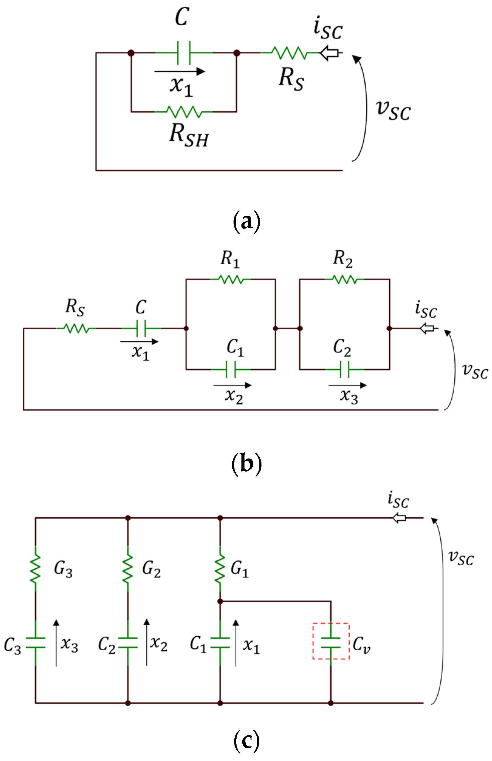
An SC equivalent circuit aims to reproduce the complex behavior exhibited by the components in transient and steady-state operation of the device. It is a common occurrence that the equivalent circuit is composed of two independent sub-circuits, with different time constants, that accommodate the electrical response of the network, according to both regimes. The only exception is the classic lossy capacitor model, shown in Figure 2a. This model results in a capacitor small-signal equivalent circuit unless high frequencies are involved; in such a case, a series inductance must be added to the equivalent circuit. Modelling the SC in this fashion has the advantage of linearity, making the analysis in the Laplace domain simple if control systems must be implemented. The limit of the resulting first-order circuit, however, is that it represents the behavior of the device through a single time constant. This is acceptable for classic electronics capacitors but fails to describe the complex dynamic response of SCs. A natural evolution of this model is given in [22], where two additional RC cells are added, as shown in Figure 2b. This model, often addressed as “dynamic” in the literature, is a third-order equivalent circuit. The individual capacitor C often assumes a large value and represents the circuit part inside the device devoted to the energy storage. This is clearly understandable by the fact that, when operated under open circuit conditions, the voltage across the SC is equal to the voltage across C, once a steady state is reached. The two RC cells account for the non-instantaneous transient response of the capacitor under pulsed current operations.

A third proposed equivalent circuit, generally addressed as “multi-cell”, is shown in Figure 2c: it is similar to the one shown in Figure 2b, but here the series of RC parallels are replaced by the parallel of the RC series. This equivalent circuit denotes the absence of a dominating capacitor accounting for a state-of-charge device; moreover, the physical interpretation of short-time transient responses, in terms of redistribution of charge inside the porous dielectric, is accounted. In [26], the authors propose this model with a small non-linearity added to one of the RC series branches. The three topologies constitute circuits that can be included easily in a time-domain simulation of a larger network the SC belongs to. The state-space representations of the classic, dynamic, and multi-cell circuits are, respectively, given in (1), (2), and (3).

$${\dot{x}}_1=\frac{1}{C}\left(i_{SC}-\frac{x_1}{R_{SH}}\right)$$

(1)

$$\{\begin{array}{c}{\dot{x}}_1=\frac{1}{C}\left(i_{SC}\right)\\ {\dot{x}}_2=\frac{1}{C_1}\left(i_{SC}-\frac{x_2}{R_1}\right)\\ {\dot{x}}_3=\frac{1}{C_2}\left(i_{SC}-\frac{x_3}{R_2}\right)\end{array}$$

(2)

$$\{\begin{array}{c}{\dot{x}}_1=\frac{1}{C_1+\left(C_v·\frac{x_1}{v_{nom}}\right)}{G}_1\left(\frac{i_{sc}+G_2\left(x_2-x_1\right)+G_3\left(x_3-x_1\right)}{\left(G_1+G_2+G_3\right)}\right)\\ {\dot{x}}_2=\frac{1}{C_2}{G}_2\left(\frac{i_{sc}+G_1\left(x_1-x_2\right)+G_3\left(x_3-x_2\right)}{\left(G_1+G_2+G_3\right)}\right)\\ {\dot{x}}_3=\frac{1}{C_3}{G}_3\left(\frac{i_{sc}+G_2\left(x_2-x_3\right)+G_1\left(x_1-x_3\right)}{\left(G_1+G_2+G_3\right)}\right)\end{array}$$

(3)

Equations (1)–(3) can be analytically integrated or, if included in a larger non-linear system (as usually is the case), can be numerically solved. Initial conditions at a steady state can be easily defined, assuming the SC is disconnected from any load (i.e., $i_{sc}\left(0\right)=0$). In (1), assuming that $R_{SH}$ is very large, results in that $v_{sc}\left(0\right)\approx x_1\left(0\right)$. In (2), the two RC branches allow discharging of the capacitors; however, the main capacitor has no path to discharge. Thus, $x_1\left(0\right)=v_{sc}\left(0\right), x_2\left(0\right)=0, \mathrm{and} x_3\left(0\right)=0$. In (3), at a steady state, no current flows through the three conductances $G_1$, $G_2$, and $G_3$. All capacitors share the same voltage, which is equal to the SC voltage, thus $x_1\left(0\right)=x_2\left(0\right)=x_3\left(0\right)=v_{sc}\left(0\right)$.

3.2. Non-Linear Dynamic Model (NLDL)

Although the simplicity of the models shown in Figure 2 is important to have an insight into the time constants of the circuit and to limit the computational costs associated with the simulation, these models fail in representing two aspects of a hybrid SC’s real behavior. The first one is related to the state of charge (SOC) of the SC. A trend that can be observed experimentally is the slower time constant of the hybrid SC, i.e., the one relative to the capacitor C, which changes drastically according to the SOC, falling rapidly once the SC reaches a threshold that usually denotes an empty SC.

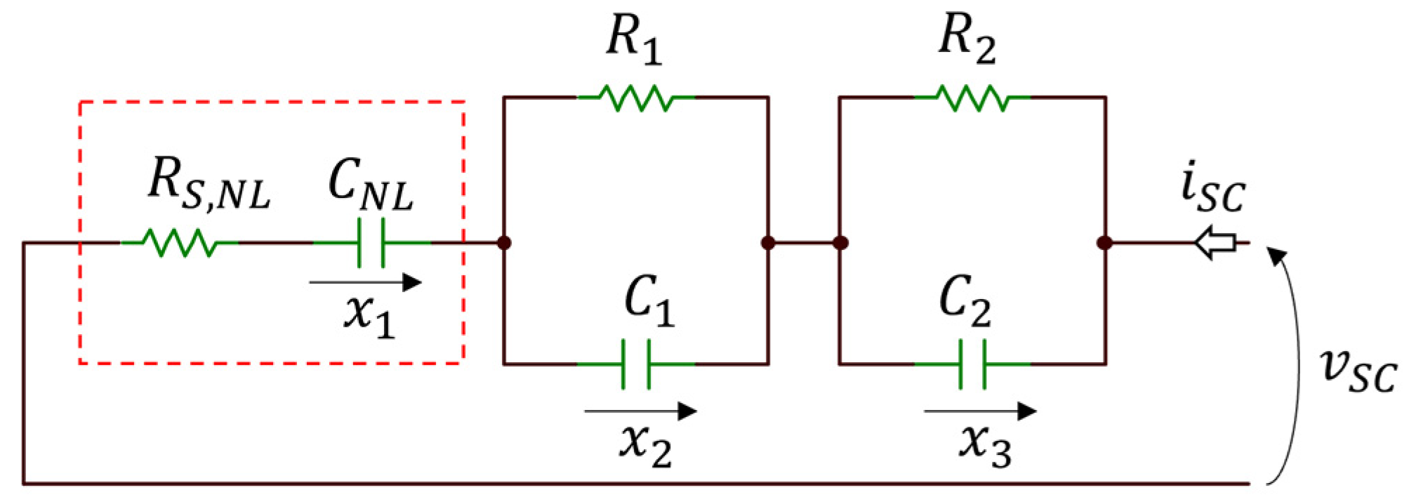
Since the energy stored inside the hybrid SC is not strictly related to the energy stored in a normal SC, the value of the main capacitor C should change according to the SOC. A proportional dependence between the capacitance and the SOC is used in this paper, by introducing a non-linearity inside the system, modeled by C_NL. The same effect is expected for the series resistance, where large voltage drops appear when the hybrid SC approaches the discharged condition. To consider this effect, the series resistance is replaced with a voltage-controlled resistance R_S,NL. The obtained model, shown in Figure 3, is non-linear and is defined by the following state-space equations, with the added non-linear relationships for the capacitor and resistor.

$$\begin{gathered} \{\begin{array}{c}{\dot{x}}_1=\frac{1}{C_{NL}\left(x_1\right)}\left(i_{SC}\right)\\ {\dot{x}}_2=\frac{1}{C_1}\left(i_{SC}-\frac{x_2}{R_1}\right)\\ {\dot{x}}_3=\frac{1}{C_2}\left(i_{SC}-\frac{x_3}{R_2}\right)\end{array} \\ {R}_{S,NL}=R_S\frac{1}{1+{\left(x_1-v_{min}\right)}^k} \\ {C}_{NL}\left(x_1\right)=C_{min}+\frac{x_1-v_{min}}{v_{nom}-v_{min}}\left(C_{max}-C_{min}\right) \end{gathered}$$

(4)

The non-linear term $R_{S,NL}$ is a hyperbole-shaped function of the current through the resistor itself, with a flection point at $v_{min}$, and a steepness gave by the $k$ term. The term $C_{NL}$ has a linear descending slope between a maximum value of capacitance $C_{max}$, when the SC is completely full, and a minimum value of capacitance $C_{min}$, when the SC is completely discharged. In general, the nominal voltage $v_{nom}$ is obtained from the SC datasheet, whereas the threshold $v_{min}$ is considered as a parameter to be optimized. Indeed, even if the relationship for $C_{NL}$ is linear, the capacitor equivalent circuit itself exhibits non-linear behavior. Moreover, the circuit is not time-invariant anymore. The resulting equivalent circuit can be classified as a grey-box model, because of the heuristic inclusion of the two non-linear components’ constitutive relationships. The general advantage of the NLDL model is its capability to represent the behavior of the physical object (the SC) under different time scales. The behavior of short transient is very different from the general charge–discharge procedure of the SC. Moreover, differently from any type of capacitor, a Hybrid SC exhibits very different behavior when the voltage across it reaches the minimum nominal value, quickly rising the series resistance. The advantage of the NLDL model is to represent all these behaviors at the same time with an equivalent circuit model that can be included in circuit simulation software easily. Lastly, it should be noted that the NLDL model considering $k=0$ and $C_{max}=C_{min}$ is equivalent to the dynamic model. This extends its compatibility to the EDLC technology as well, as shown from the references in Table 2.

3.3. Neural Estimator (NE)

Purely black-box approaches are implemented to represent the dynamic behavior of the component as well. The advantage of these models is the algorithmic approach that can be used for their construction. Neural models can be used to define the relationship between the instantaneous current and the instantaneous voltages across the SC.

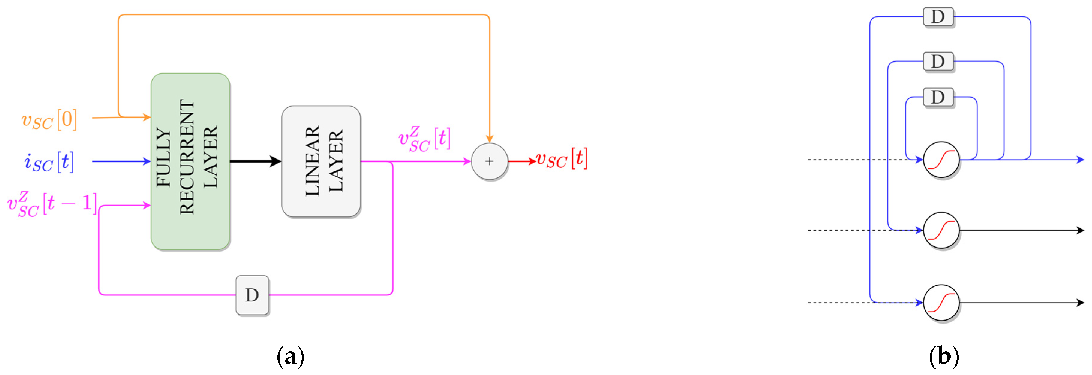
Obviously, the neural model should be chosen among the architectures featuring dynamic response (i.e., neural networks with memory). Several very complex neural network architectures are available in the literature. However, considering the necessity of including this model inside the simulation of a larger network (e.g., a time-domain simulation of a circuit or a Monte Carlo analysis), the reduction in computational complexity must be considered. The core of the architecture proposed for this NE, as shown in Figure 4a, is a fully recurrent layer, shown in Figure 4b. This layer is composed of non-linear neurons whose output is fed back as input (after a delay) to all the neurons of the layer. This implements a dynamical system of non-linear state equations. The output of the Fully Recurrent Layer is fed to a linear output layer, with a feedback loop. The reason for this loop is to give the NE the additional information about the actual SOC of the supercapacitor. As can be seen in Figure 4a, even if the output of the NE is the voltage across the SC, the output of the neural part is the quantity $v_{SC}^Z\left[t\right]$, which is defined as $v_{SC}^Z\left[t\right]=v_{SC}\left[t\right]-v_{SC}\left[0\right]$. This quantity is, in fact, the deviation of the supercapacitor voltage from its initial condition $v_{SC}\left[0\right]$. Training the two neural layers to predict this quantity (instead of the true voltage) is required because, differently from the equivalent-circuit based models, here, it is impossible to translate an electrical initial condition in the inner parameters of a black-box model. Thus, the initial condition is removed before the data are processed and returned at the output through a sum block. Since the non-linear behavior of the SC is strongly related to the initial conditions, this quantity is used as input for the NE as well. Lastly, to better reflect the fact that the neural layers represent only the deviation from the initial condition (and thus should have a steady-state null output), all biases are forced to zero in the neurons of the two layers. Designed with these observations in mind, the NE can be sized easily to accommodate the fitting of the proposed problem. However, being in a black-box system, it suffers from the inability of obtaining any insight on the system, apart from its direct output. Equivalent circuit models, on the other hand, can be used to assess commutation losses, state of charge, and individual time constants. This cannot be performed by a black-box model unless specifically trained to do so with additional data. The Neural Estimator is implemented as a customized “layerecnet” in Matlab R2021b environment, provided with the feedback loops shown in Figure 4 and decurted of the biases to avoid convergence towards non-physical solutions. Training is performed using backpropagation through time for gradient calculation (due to the dynamic nature of the NN) and a classic Levenberg-Marquardt algorithm for LSQ minimization.

3.4. Model Identification Algorithm

The model identification is performed by minimizing the difference, in terms of response, between the reference data and the model, for a given excitation, which is the SC current $i_{sc}\left(t\right)$; the circuit response is the voltage across the SC $v_{sc}\left(t\right)$. Thus, the goal of the model identification approach is to minimize the error vector:

$$e\left[t\right]=v_{sc}^S\left[t\right]-v_{sc}^R\left[t\right]$$

(5)

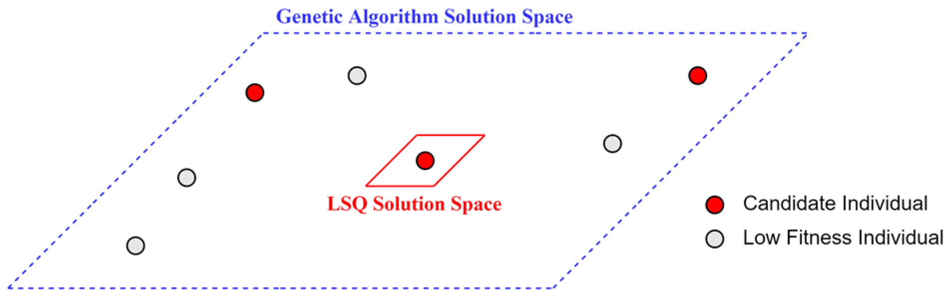
where the superscripts S and R denote the simulated and reference values of the SC voltages. This problem could be simply approached by the least squares (LSQ) solver, but this could yield sub-optimal solutions. Non-linear least-squares problems can exhibit local minima where the identification algorithm might stop, halting before reaching an optimal solution. Moreover, the separation of the time constants of the circuit might not occur if a greedy optimization algorithm is used from all the optimization process. For these two reasons, a hybrid strategy, composed of the cascade of two optimization systems, was implemented, as shown in Figure 5. The first stage investigates a wide solution space utilizing a highly explorative genetic algorithm, for which the main parameters are reported in

Table 3. Cost functions in (6) for the specific problem.

	Classic	Dynamic	Multicell	NLDL
$c{f}_{\tau 1}$	0	$\frac{R_1{C}_1}{R_{S}C}$	$\frac{G_1{C}_2}{G_2{C}_1}$	$\frac{R_1{C}_1}{R_{S,NL}^{*}{C}_{NL}^{*}}$
$c{f}_{\tau 2}$	0	$\frac{R_2{C}_2}{R_{S}C}$	$\frac{G_1{C}_3}{G_3{C}_1}$	$\frac{R_2{C}_2}{R_{S,NL}^{*}{C}_{NL}^{*}}$

. The cost function associated with each individual of the genetic pool is the combination of three contributions.

$$cf=c{f}_{err}+c{f}_{\tau 1}+c{f}_{\tau 2 }$$

(6)

where $c{f}_{err}$ is the absolute sum of all elements constituting the error vector in (5). The cost functions $c{f}_{\tau 1}$ and $c{f}_{\tau 2}$ account for the separation of the time constants of the circuits and are differently calculated, according to the used model. For the four models proposed, the expressions are given in Table 3. Since the time constants in the non-linear dynamic model change according to the instantaneous electrical quantities in the circuit, average values $R_{S,NL}^{*}{C}_{NL}^{*}$, over the whole simulation, are used. The genetic algorithm generates several candidate solutions that need to be refined further by a local search algorithm. For each of these candidate solutions, the sub-space of the solution space centered on the individual is defined. In this sub-space, an LSQ refinement of the solution is obtained through a Levenberg–Marquardt algorithm. Solutions refined by the LSQ are then ranked for mean absolute error, and the best performing one is considered as the identified model.

3.5. Data Acquisition: Experimental Workbench Layout

An experimental workbench to acquire data representing the electrical behavior of the hybrid supercapacitor SC4R2V402F24 supercapacitors by Gonghe Electronics was implemented. The characteristics of the supercapacitor are those reported in

Table 4. Characteristics of the SC4R2V402F24 hybrid supercapacitor employed for model retrieval.

Parameter	Value
Rated Voltage	4.2 V
Rated Capacity	4000 F
Continuous Maximal Discharging Current	6 A
Pulse Discharging Current	30 A

. This supercapacitor has good stability and chemical reversibility which makes it suitable for military and aerospace applications. After 20,000 charging/discharging cycles, the capacitor maintains 95% of the initial capacity.

To apply charging and discharging cycles to the supercapacitor, the experimental layout shown in Figure 6 was employed. The supercapacitor is part of a circuit that is connected to a DSC DP15-60H charger and a RIGOL DL3021 discharger. Both instruments are automatically controlled by a NI LabVIEW 2017 interface specially developed for this application. The SC Voltages and currents are continuously monitored: during discharging, the RIGOL directly interfaces with LabVIEW for the acquisition of both measurements; during charging, the current is deducted by measuring the voltage drop at the ends of a 188 mΩ resistance, amplified by a TI INAP128, and converted to a digital value through an Arduino UNO device.

3.6. Identification and Validation Procedures Datasets

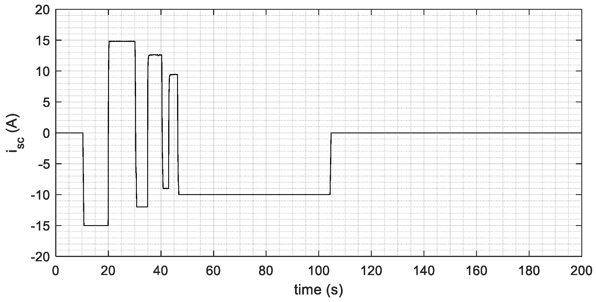
The datasets used for the identification and validation are acquired using the setup described in the previous section. Both datasets are composed of the sampling of an excitation vector (current) and a response vector (voltage). The waveform used, depicted in Figure 7, aims to show both the fast transient response of the SC (through very rapid steps) and the slow discharging dynamic (through a long constant section of absorbed current). The data are acquired in batches of 2000 samples with a timestep of 100 ms using a current waveform 200 s long as the excitation. The current waveform is used repeatedly to generate different datasets, which are different due to the different states of charge of the SC. Most importantly, the discharge is performed up to a point where the non-linear behavior of the SC exhibits a strong increase in the series resistance. The identification and the validation datasets consist, respectively, of 8000 samples (four curves) and 2000 samples (one curve) of couples $\left\{i_{SC}^R,v_{SC}^R\right\}$. The identification dataset is used for the identification procedure of the circuit models, as described in Section 3.1 and Section 3.2, and for the training of the NE described in Section 3.3. The validation dataset is used as an independent set of data and is never utilized to train the model/NE. This has been done to check if the identification procedure managed to generate a model, NE was able to generalize the behavior of the system, or if it simply managed to memorize the data patterns.

4. Results and Discussion

In this section, the results for the identification and validation procedure are discussed for the four circuit models and the neural estimator.

4.1. Circuit Models Comparison

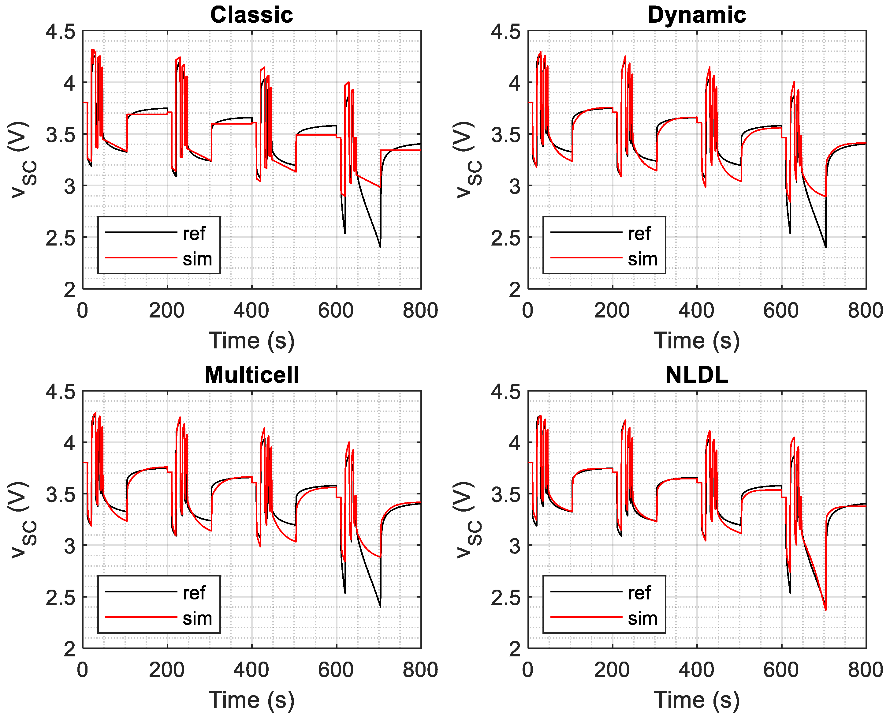
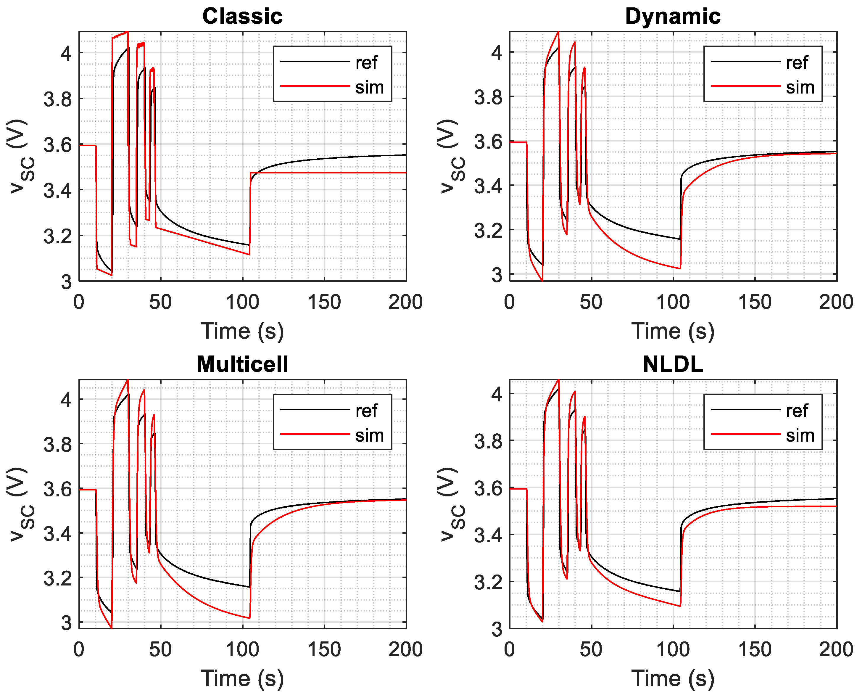
The response of the identified models on the identification dataset is shown in Figure 8, and the response concerning the validation dataset is shown in Figure 9.

As expected, the classic model is not able to reproduce the slow and the fast response of the SC circuit at the same time, resulting in an average behavior that neither fits the transient nor the steady-state response. Dynamic and multicell circuits both exhibit good responses on the transient behavior and achieve very accurate results in terms of steady-state response (with an almost null error on the validation set). However, both the Dynamic and multicell fail in reproducing the SC strong non-linear behavior which arises when the voltage across the tested device drops to low values (i.e., below 3 V). The NLDL model is the only one correctly reproducing this non-linear behavior. However, this is achieved with higher complexity and slightly lower performance in terms of steady-state response, as shown in Figure 9 The parameters for the identified circuit models are shown in

Table 5. Identified parameters for the different models, errors on the identification and validation datasets, R-squared regression error.

Model	Parameters	Id. MSE	Val. MSE	${\mathit{R}}^2$
Classic	$$\begin{gathered} C=4.8120\times {10}^3 F \\ {R}_S=3.5971\times {10}^{-2}\mathsf{\Omega } \\ {R}_{SH}=9.6224\times {10}^4\mathsf{\Omega } \end{gathered}$$	$1.9910\times {10}^{-2}$	$1.0075\times {10}^{-2}$	0.7505
Dynamic	$$\begin{gathered} C=1.1419\times {10}^4 F \\ {C}_1=9.3870\times {10}^2 F \\ {C}_2=1.8413\times {10}^1 F \\ {R}_1=2.0080\times {10}^{-2}\mathsf{\Omega } \\ {R}_2=3.0436\times {10}^{-2}\mathsf{\Omega } \\ {R}_S=2.5328\times {10}^{-3}\mathsf{\Omega } \end{gathered}$$	$1.0415\times {10}^{-2}$	$5.4955\times {10}^{-3}$	0.8909
Multicell	$$\begin{gathered} C_v=1.7809\times {10}^2 F \\ {C}_1=3.5554\times {10}^4 F \\ {C}_2=1.2628\times {10}^1 F \\ {C}_3=1.5601\times {10}^{-7} F \\ {G}_1=1.1281\times {10}^1 S \\ {G}_2=1.7906\times {10}^1 S \\ {G}_3=3.6587\times {10}^2 S \end{gathered}$$	$1.0227\times {10}^{-2}$	$5.6761\times {10}^{-3}$	0.9027
NLDL	$$\begin{gathered} C_{max}=1.3330\times {10}^4 F \\ {C}_1=1.4521\times {10}^3 F \\ {C}_2=1.8001\times {10}^1 F \\ {R}_1=1.2120\times {10}^{-2}\mathsf{\Omega } \\ {R}_2=3.1241\times {10}^{-2}\mathsf{\Omega } \\ {R}_S=5.1129\times {10}^{-2}\mathsf{\Omega } \\ {v}_{min}=2.4605\times {10}^{0 }V \\ k=8.5126\times {10}^1 \\ {C}_{min}=2.1091\times {10}^{-3} F \end{gathered}$$	$4.2111\times {10}^{-3}$	$2.3709\times {10}^{-3}$	0.9590

, along with the MSE on the identification and validation datasets.

4.2. Neural Estimator

Identification of the Neural Estimator is performed similarly to the identification of the circuit model. The inner parameters are defined by using a training algorithm (backpropagation for the gradient definition, and Levenberg–Marquardt for the minimization of the resulting LSQ problem) that minimizes the error between the simulated data and the reference data, on the identification dataset. Once the NE is identified, its performance is evaluated on the validation dataset. The optimal sizing of the NE was determined empirically, using a technique described in [9,34] to prevent the data overfitting and resulted in four neurons in the fully recurrent layer.

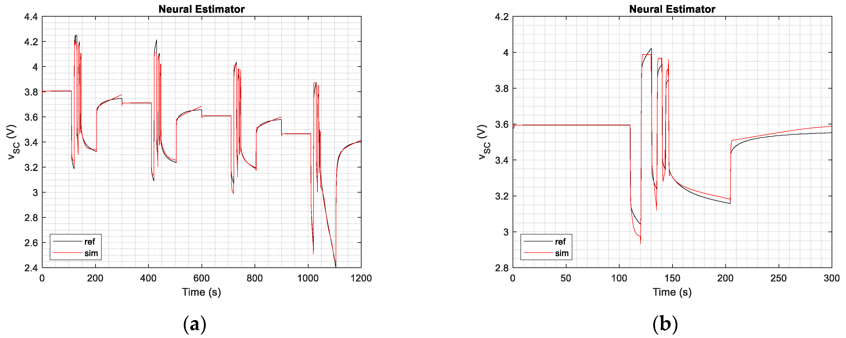
This approach is notably different from the circuit model technique; the data are artificially padded with zeros in the initial region to enlarge the steady-state part. This gives a larger weight, in terms of training, to these regions. Results on the identification and validation dataset are shown in Figure 10a,b, respectively. The neural estimator correctly predicts the strong non-linearity and the discharge behavior, but is less accurate in predicting the steady-state operation, especially once the discharge transient is over. The MSE is equal to $7.0338\times {10}^{-4}$ in the identification dataset, and $8.1566\times {10}^{-4}$ in the validation dataset. The regression error $R^2$ is 0.9895.

4.3. Statistical Robustness of NLDL Identification

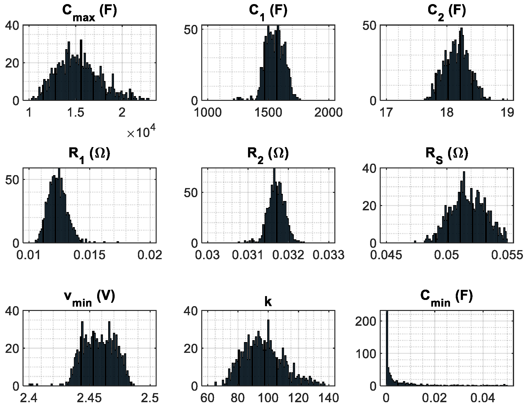
Identification of a non-linear model must be validated statistically by verifying the robustness of the found solution with respect to noisy input data. This validation is performed by applying a random noise to the reference data, acquired experimentally, and repeating the identification procedure several times, recording the average parameters and their standard deviation. For this purpose, the identification procedure of the NLDL was repeated 1000 times with a random noise of 100 mV amplitude added to the dataset. The average parameters obtained, and their standard deviation can be found in

Table 6. Statistical analysis results over 1000 identification runs, average and standard deviation values for the NLDL model.

	Average Parameter	Standard Deviation
$C_{max}$	$1.527715\times {10}^4$	$2.285536\times {10}^3$
$C_1$	$1.530628\times {10}^3$	$1.981729\times {10}^2$
$C_2$	$1.815956\times {10}^1$	$2.007367\times {10}^{-1}$
$R_1$	$1.233306\times {10}^{-2}$	$8.516536\times {10}^{-4}$
$R_2$	$3.140747\times {10}^{-2}$	$2.315775\times {10}^{-3}$
$R_S$	$5.167659\times {10}^{-2}$	$2.130498\times {10}^{-3}$
$v_{min}$	$2.456013\times {10}^0$	$2.207561\times {10}^{-2}$
$k$	$9.562971\times {10}^1$	$1.535824\times {10}^1$
$C_{min}$	$5.484666\times {10}^{-3}$	$9.681274\times {10}^{-3}$

. The histogram for the individual parameters can be seen in Figure 11. As can be seen, all parameters exhibit Gaussian-like distribution with the exception of $C_{min}$, which tends to flatten near the quasi-zero values. Standard deviation of the parameters is not negligible, especially for the ones relative to the non-linear elements. This variance confirms that the solution space of the non-linear identification problem features several local minima, for which an advanced identification algorithm such as the one used in this work is necessary to avoid sub-optimal solutions.

5. Conclusions

Two accurate techniques in modelling the dynamic and non-linear behavior of a hybrid supercapacitor were presented in this work. The first technique enlarges and increases the accuracy of the equivalent circuit approach by introducing two specific non-linearities dependent on the state-of-charge of the device. These non-linearities better represent (with respect to already known techniques) the large behavioral change exhibited by a hybrid SC when its voltage is close to the point of maximum discharge. The second technique uses a recursive neural network to create a neural estimator able to represent the divergence between the initial conditions and the final conditions of the SC states.

Both the investigated and proposed techniques are new and can be used in time-domain simulation of an electrical network including SCs. The techniques based on the NLDL equivalent circuit give an interesting insight into the SC inner structure and can be used to assess the power losses. The voltage on the main capacitor can be related directly to the state-of-charge. However, this model requires numerical integration to be performed and the complexity of the calculations depends on the implementation environment. The NE based technique embeds the integration in the inner operations of the recursive layer neurons, making this model simple to use, but its parameters (weights and biases) do not allow any insight into the inner structure of the device.

Both techniques achieve high accuracy and generalization capabilities, resulting in a set of valuable tools for the simulation of electrical circuits, power converters, or stand-alone devices including SCs of the hybrid family.

As future development of this research, the performance of the proposed non-linear dynamic models will be evaluated for different SC technologies. The obtained high-accuracy models for hybrid SCs will be employed to pilot the design phase of an SC pack solution to be applied in micro-mobility contexts, for implementation as an energy storage system on lightweight, sustainable electric vehicles, such as e-kick scooters or pedelecs.

References

- Simon, P.; Gogotsi, Y. Materials for electrochemical capacitors. Nat. Mater. 2008, 7, 845–854. [Google Scholar] [CrossRef] [Green Version]
- Ouramdane, O.; Elbouchikhi, E.; Amirat, Y.; Gooya, E.S. Optimal Sizing and Energy Management of Microgrids with Vehicle-to-Grid Technology: A Critical Review and Future Trends. Energies 2021, 14, 4166. [Google Scholar] [CrossRef]
- Parvini, Y.; Vahidi, A.; Fayazi, S.A. Heuristic Versus Optimal Charging of Supercapacitors, Lithium-Ion, and Lead-Acid Batteries: An Efficiency Point of View. IEEE Trans. Control. Syst. Technol. 2017, 26, 167–180. [Google Scholar] [CrossRef]
- Prasad, R.; Kothari, K.; Mehta, U. Flexible Fractional Supercapacitor Model Analyzed in Time Domain. IEEE Access 2019, 7, 122626–122633. [Google Scholar] [CrossRef]
- Miniguano, H.; Barrado, A.; Fernández, C.; Zumel, P.; Lázaro, A. A General Parameter Identification Procedure Used for the Comparative Study of Supercapacitors Models. Energies 2019, 12, 1776. [Google Scholar] [CrossRef] [Green Version]
- Navarro, G.; Nájera, J.; Torres, J.; Blanco, M.; Santos, M.; Lafoz, M. Development and ex-perimental validation of a supercapacitor frequency domain model for industrial energy applications considering dynamic behaviour at high frequencies. Energies 2020, 13, 1156. [Google Scholar] [CrossRef] [Green Version]
- Saha, P.; Dey, S.; Khanra, M. Modeling and State-of-Charge Estimation of Supercapacitor Considering Leakage Effect. IEEE Trans. Ind. Electron. 2019, 67, 350–357. [Google Scholar] [CrossRef]
- Ceraolo, M.; Lutzemberger, G.; Poli, D. State-Of-Charge Evaluation of Supercapacitors. J. Energy Storage 2017, 11, 211–218. [Google Scholar] [CrossRef]
- Lozito, G.M.; Salvini, A. Swarm intelligence based approach for efficient training of regressive neural networks. Neural Comput. Appl. 2019, 32, 10693–10704. [Google Scholar] [CrossRef]
- Coco, S.; Laudani, A.; Pulcini, G.; Fulginei, F.R.; Salvini, A. Optimization of multistage depressed collectors using fem and parallel algorithm MeTEO. COMPEL—Int. J. Comput. Math. Electr. Electron. Eng. 2013, 32, 1955–1963. [Google Scholar] [CrossRef]
- Conway, B.E. Electrochemical Supercapacitors: Scientific Fundamentals and Technological Applications; Springer: New York, NY, USA, 1999. [Google Scholar]
- Conway, B. Transition from ’supercapacitor’ to ’battery’ behavior in electrochemical energy storage. J. Electrochem. Soc. 2002, 138, 1539. [Google Scholar] [CrossRef]
- Naoi, K.; Naoi, W.; Aoyagi, S.; Miyamoto, J.-I.; Kamino, T. New Generation Nanohybrid Supercapacitor. Acc. Chem. Res. 2013, 46, 1075–1083. [Google Scholar] [CrossRef] [PubMed]
- Ferraro, D.; Andolina, G.M.; Campisi, M.; Pellegrini, V.; Polini, M. Quantum supercapacitors. Phys. Rev. B 2019, 100, 075433. [Google Scholar] [CrossRef] [Green Version]
- Santhibhushan, B.; Khan, M.S.; Bohat, V.K.; Srivastava, A.; Khan, S. Quantum Capacitance Estimations of Pyrrolic-Rich Graphene for Supercapacitor Electrodes. IEEE Trans. Nanotechnol. 2017, 17, 205–211. [Google Scholar] [CrossRef]
- Chemali, E.; Preindl, M.; Malysz, P.; Emadi, A. Electrochemical and Electrostatic Energy Storage and Management Systems for Electric Drive Vehicles: State-of-the-Art Review and Future Trends. IEEE J. Emerg. Sel. Top. Power Electron. 2016, 4, 1117–1134. [Google Scholar] [CrossRef]
- Lasrado, D.; Ahankari, S.; Kar, K.K. Global Trends in Supercapacitors. In Graphite Intercalation Compounds I; Springer Series in Materials Science: Cham, Switzerland, 2021; Volume 313, pp. 329–365. [Google Scholar]
- Technical Bulletin for Maxwell Double Layer Supercapacitor. Available online: https://maxwell.com/products/ultracapacitors/cells/ (accessed on 13 October 2021).
- Technical Bulletin for Nesscap Pseudocapacitor. Available online: https://www.mouser.com/datasheet/2/257/CE_2017_Datasheet_2_3V50F_Pseudo_3001969_EN_1-1274211.pdf (accessed on 13 October 2021).
- Technical Bulletin for Taiyo Yuden Hybrid Supercapacitor. Available online: https://www.mouser.it/new/taiyo-yuden/taiyoyudensupercaps/ (accessed on 13 October 2021).
- Technical Bulletin for Ghenergy New Generation Supercapacitor. Available online: http://en.gongheenergy.com/20180404b/products/20353218.html (accessed on 13 October 2021).
- Zhang, L.; Wang, Z.; Hu, X.; Sun, F.; Dorrell, D. A comparative study of equivalent circuit models of ultracapacitors for electric vehicles. J. Power Sources 2015, 274, 899–906. [Google Scholar] [CrossRef]
- Zhang, L.; Hu, X.; Wang, Z.; Sun, F.; Dorrell, D. A review of supercapacitor modeling, estimation, and applications: A control/management perspective. Renew. Sustain. Energy Rev. 2018, 81, 1868–1878. [Google Scholar] [CrossRef]
- Parvini, Y.; Siegel, J.; Stefanopoulou, A.G.; Vahidi, A. Supercapacitor Electrical and Thermal Modeling, Identification, and Validation for a Wide Range of Temperature and Power Applications. IEEE Trans. Ind. Electron. 2015, 63, 1574–1585. [Google Scholar] [CrossRef]
- Chai, R.; Zhang, Y. A Practical Supercapacitor Model for Power Management in Wireless Sensor Nodes. IEEE Trans. Power Electron. 2014, 30, 6720–6730. [Google Scholar] [CrossRef]
- Buller, S.; Thele, M.; De Doncker, R.; Karden, E. Impedance-based simulation models of supercapacitors and Li-ion batteries for power electronic applications. In Proceedings of the 38th IAS Annual Meeting on Conference Record of the Industry Applications Conference; IEEE: New York, NY, USA, 2003; Volume 41, pp. 742–747. [Google Scholar] [CrossRef]
- Liu, K.; Zhu, C.; Lu, R.; Chan, C.C. Improved Study of Temperature Dependence Equivalent Circuit Model for Supercapacitors. IEEE Trans. Plasma Sci. 2013, 41, 1267–1271. [Google Scholar] [CrossRef]
- Şahin, M. Recep Tayyip Erdoğan University Modelling of Supercapacitors Based on Simplified Equivalent Circuit. CPSS Trans. Power Electron. Appl. 2021, 6, 31–39. [Google Scholar] [CrossRef]
- Zhao, Y.; Xie, W.; Fang, Z.; Liu, S. A parameters identification method of the equivalent circuit model of the supercapacitor cell module based on segmentation optimization. IEEE Access 2020, 8, 92895–92906. [Google Scholar] [CrossRef]
- Buller, S.; Karden, E.; Kok, D.; De Doncker, R.W. Modeling the dynamic behavior of supercapacitors using impedance spectroscopy. IEEE Trans. Ind. Appl. 2002, 38, 1622–1626. [Google Scholar] [CrossRef]
- Rizoug, N.; Bartholomeus, P.; Le Moigne, P. Modeling and Characterizing Supercapacitors Using an Online Method. IEEE Trans. Ind. Electron. 2010, 57, 3980–3990. [Google Scholar] [CrossRef]
- Weddell, A.; Merrett, G.; Kazmierski, T.J.; Al-Hashimi, B.M. Accurate Supercapacitor Modeling for Energy Harvesting Wireless Sensor Nodes. IEEE Trans. Circuits Syst. II Express Briefs 2011, 58, 911–915. [Google Scholar] [CrossRef] [Green Version]
- Morandi, A.; Lampasi, A.; Cocchi, A.; Gherdovich, F.; Melaccio, U.; Ribani, P.L.; Rossi, C.; Soavi, F. Characterization and Model Parameters of Large Commercial Supercapacitor Cells. IEEE Access 2021, 9, 20376–20390. [Google Scholar] [CrossRef]
- Fulginei, F.R.; Laudani, A.; Salvini, A.; Parodi, M. Automatic and Parallel Optimized Learning for Neural Networks performing MIMO Applications. Adv. Electr. Comput. Eng. 2013, 13, 3–12. [Google Scholar] [CrossRef]
Figure 1.
Different types of models employed in the literature to reproduce the stationary and transient behavior of SC technologies. SC terminals are denoted by the squared A and B nodes. (a) Simplified model. (b) RC branches series model. (c) RC transmission model. (d) RC branches parallel model. (e) Classical RC battery model. (f) General high-order model.
Figure 2.
Equivalent circuit models and main electrical variables for SC devices: classic model (a), dynamic model (b), and multi-cell model (c).
Figure 3.
Proposed SC non-linear dynamic model, featuring non-linear components for the main capacitor and main series resistance.
Figure 4.
Neural Estimator. (a) Neural Estimator architecture, highlighting inputs and outputs. (b) Detail on the connection paradigm used in a fully recurrent layer, where only the feedback connections of the first neuron are shown for clarity.
Figure 5.
Hybrid model identification strategy featuring the maximal Genetic Algorithm solution space and one of the sub-spaces, where the LSQ algorithm refines each one of the candidate solutions.
Figure 6.
Lab setup utilized to the hybrid SC, considering both phases of charging and discharging.
Figure 7.
Base current waveform used for the SC discharge procedure.
Figure 8.
Real voltage trend for the SC and the corresponding best-fitting curve obtained by the four circuit models, applied to the training dataset.
Figure 9.
Real voltage trend for the SC and the corresponding best-fitting curve obtained by the four circuit models, applied to the validation dataset.
Figure 10.
Real voltage trend for the SC and corresponding best-fitting curve obtained by the neural estimator, applied to the training (a) and testing (b) datasets.
Figure 11.
Histogram representation of the parameters found in the 1000 individual runs of the identification procedure.