
Accuracy of Simplified Modelling Assumptions on External and Internal Driving Forces in the Building Energy Performance Simulation


Abstract
:1. Introduction
1.1. Validation Techniques of the Building Energy Models
1.2. Validation Studies of the EN ISO 52016-1 Hourly Model
1.3. Aims of the Research Work
- detect the modelling assumptions of the simplified hourly method on different levels, such as the modelling of the thermo-physical phenomena, the neglecting of some physical phenomena, the determination or the temporal discretisation of specific calculation parameters, or the definition of calculation boundary conditions,
- minimise the uncertainty in the validation of a calculation method due to inconsistencies in the input data,
2. Materials and Methods
2.1. Simplified Modelling of External Driving Forces
2.1.1. Convective Heat Transfer
2.1.2. Longwave Radiation Heat Transfer
2.1.3. Solar (Shortwave) Radiation
2.2. Simplified Modelling of Internal Driving Forces
2.2.1. Convective Heat Transfer
2.2.2. Longwave Radiation Heat Transfer
2.2.3. Solar (Shortwave) Radiation
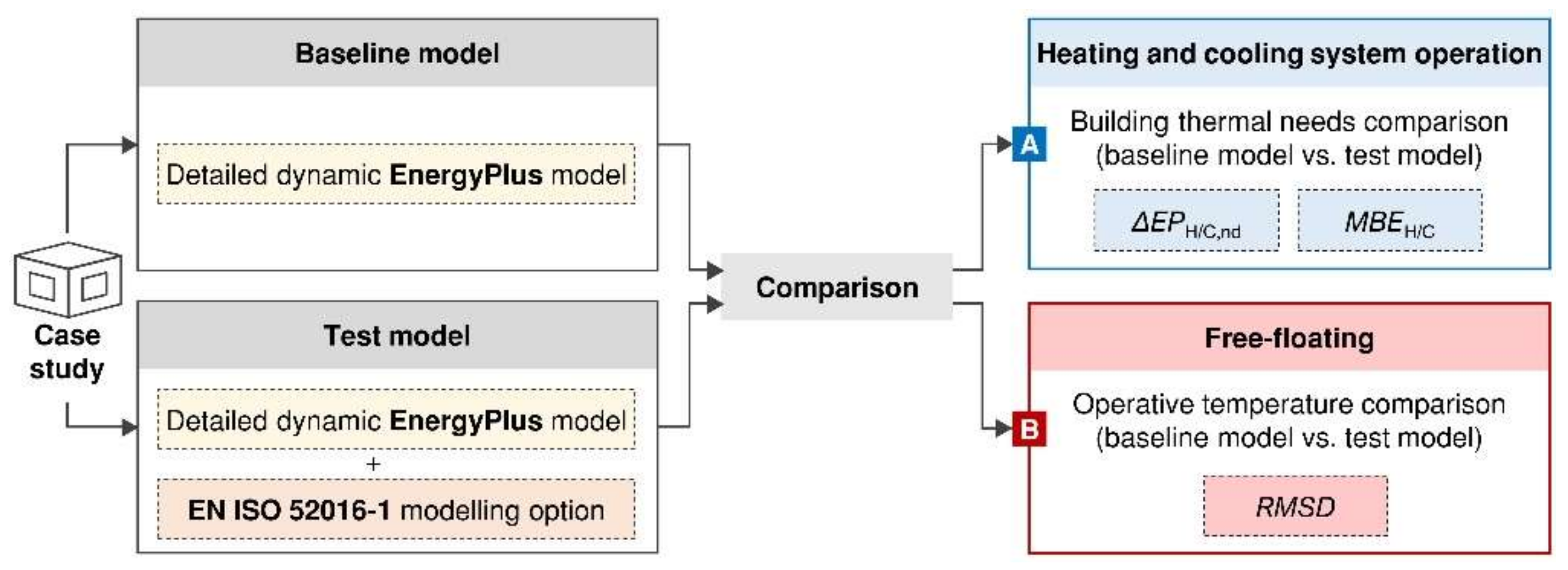
2.3. Methodology
3. Application
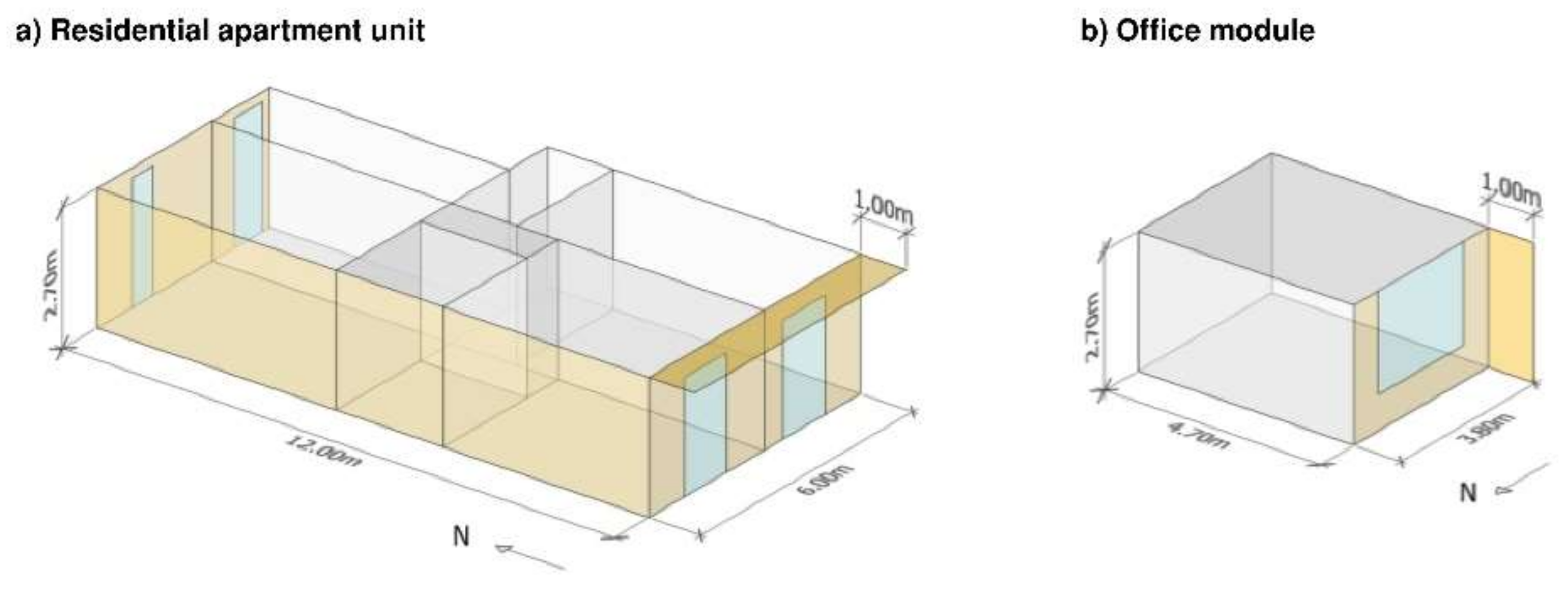
3.1. Case Studies
3.2. Modelling Options
- HC-Vw-av. The effect of a lack of detailed input data regarding the wind speed was assessed. In particular, the convective heat transfer coefficient was considered time-dependent and was calculated by means of the TARP algorithm [24]. Differently from the baseline model, the forced component is calculated by implementing annual average wind speed values; specifically, wind speeds of 0.9 and 3.8 m·s−1 were used for Milan and Palermo, respectively.
- HC-V. The effect of the formulation specified in Equation (2) for the hc,ext determination was evaluated. The convective heat transfer coefficient was considered variable on a timestep basis, and the site hourly wind speed was used.
- HC-Cw-av. The annual average wind speed was implemented in Equation (2) to calculate an average heat transfer coefficient, assumed constant over the simulation period.
- HC-Cst. The effect of the hc,ext standard values was evaluated, assuming a constant convective heat transfer coefficient equal to 20 W·m−2·K−1 over the simulation period, calculated by means of the reference wind speed value of 4 m·s−1 (Equation (2)).
- SKY. The influence of the direct sky temperature model for the apparent sky temperature calculation was assessed; specifically, the sky temperature was assumed 11 °C below the outdoor air temperature.
- HR. In EnergyPlus, the external net longwave radiation heat flux is calculated by applying the Stefan-Boltzmann law. Thus, the definition of the radiative heat transfer coefficients as input values was not possible. To assess the influence of the linearisation of the longwave heat transfer (Equation (4)), a simple modelling strategy was applied. Firstly, the outdoor surface emittances were set equal to 0 to annul the external longwave heat transfer automatically calculated by EnergyPlus. Then, an additional heat balance term, calculated as specified in Equation (4), was added to the external surface of the envelope components. The standard radiative heat transfer coefficient (hr,ext) equal to 4.14 W·m−2·K−1 was used, and was calculated by assuming a surface emissivity equal to 0.9 and a reference mean temperature of 0 °C [23]. The EnergyPlus’s calculated view factor between the surface and the sky (Fsky) was assumed, as well as the Clark and Allen [27] calculated sky temperature.
- HR-EU. The parameters described for the HR test model were used in this step, while the apparent sky temperature was calculated as direct difference from outdoor air (11 °C).
- GV-EU. The effect of considering the solar radiation entering the thermal zone as all shortwave radiation was assessed. To this purpose, the direct solar transmission coefficient of windows was set equal to the g-value (at normal incidence), while 0 was assumed for the absorption factor. The glazing solar properties were considered time- and solar angle-independent, by assuming a constant exposure factor (FW in Equation (6)) equal to 0.9 over the simulation period [2].
- GV-ITA. The parameters described for the GV-EU test model were used in this step, while the glazing solar properties were considered solar angle- and time-dependent, by assuming a variable exposure factor (FW in Equation (6)) calculated by means of the Italian National Annex approach [28].
- HC-Cst. A constant value of the convective heat transfer coefficient was considered over the simulation period, whose determination depends on the direction of the heat flow. As specified by the EN ISO 6946 technical standard [23], the hc,int values were assumed equal to 5.0, 2.5 and 0.7 W·m−2·K−1, for horizontal, upward and downward heat fluxes, respectively.
- IG. Firstly, only the convective fraction of internal gains (occupancy, appliances, and lighting) was set as input data in the EnergyPlus model (test model). Then, their radiative fraction was directly applied to the internal surfaces as additional heat balance term, calculated for each timestep as in Equation (9).
- BR. The assumption of EN ISO 52016-1 to not consider a fraction of solar radiation that is reflected back outside the zone from windows was evaluated. To this purpose, the “lost” solar radiation (Equation (13)) was added as an additional heat balance term to each surface, proportionally to the respective surface areas and solar absorption factors (Equation (12)).
- UD. The effect of the uniform distribution of solar radiation on the internal surfaces, specified by the EN ISO 52016-1 hourly method, was evaluated. A simple modelling procedure was applied; the internal surface solar absorption was set equal to 0 to annul the absorbed solar radiation automatically calculated by EnergyPlus. Then, the global (beam plus diffuse) solar radiation entering the zone at each timestep was distributed uniformly on the internal surfaces (Equation (11)). Solar heat gains were considered all radiant heat gains.
- UD-CSG. The influence of the fraction of solar radiation directly transferred to the internal air as convective heat gain was evaluated. The modelling approach of UD was applied. Differently from the UD test model, the solar radiation distributed over the internal surfaces was decreased by a 10%, considered as a convective heat gain.
4. Results
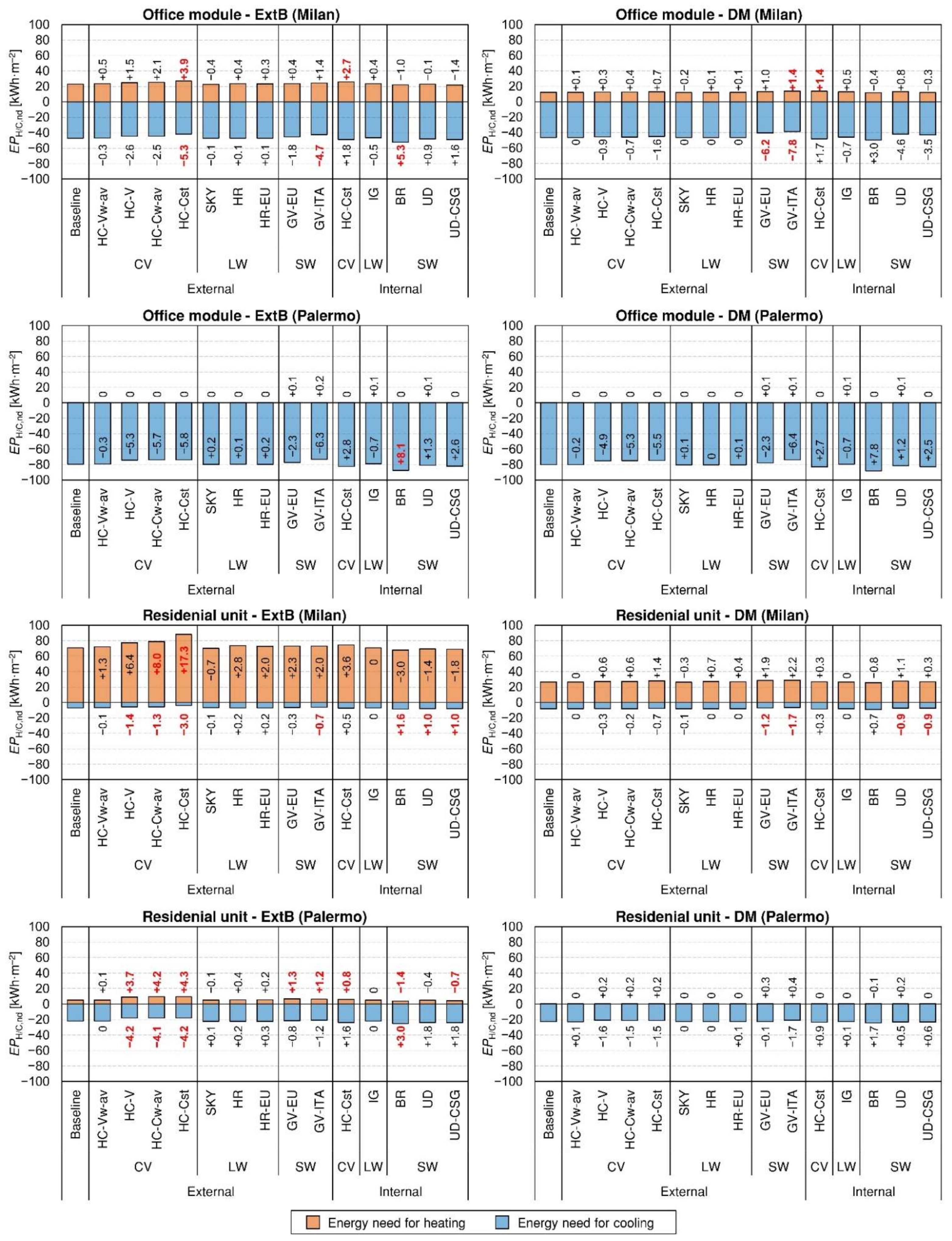
4.1. Energy Needs Evaluation
4.1.1. Simplified Modelling of the External Driving Forces
4.1.2. Simplified Modelling of the Internal Driving Forces
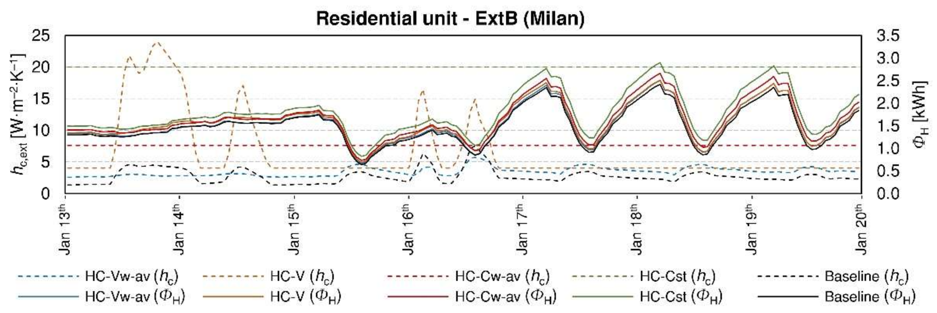
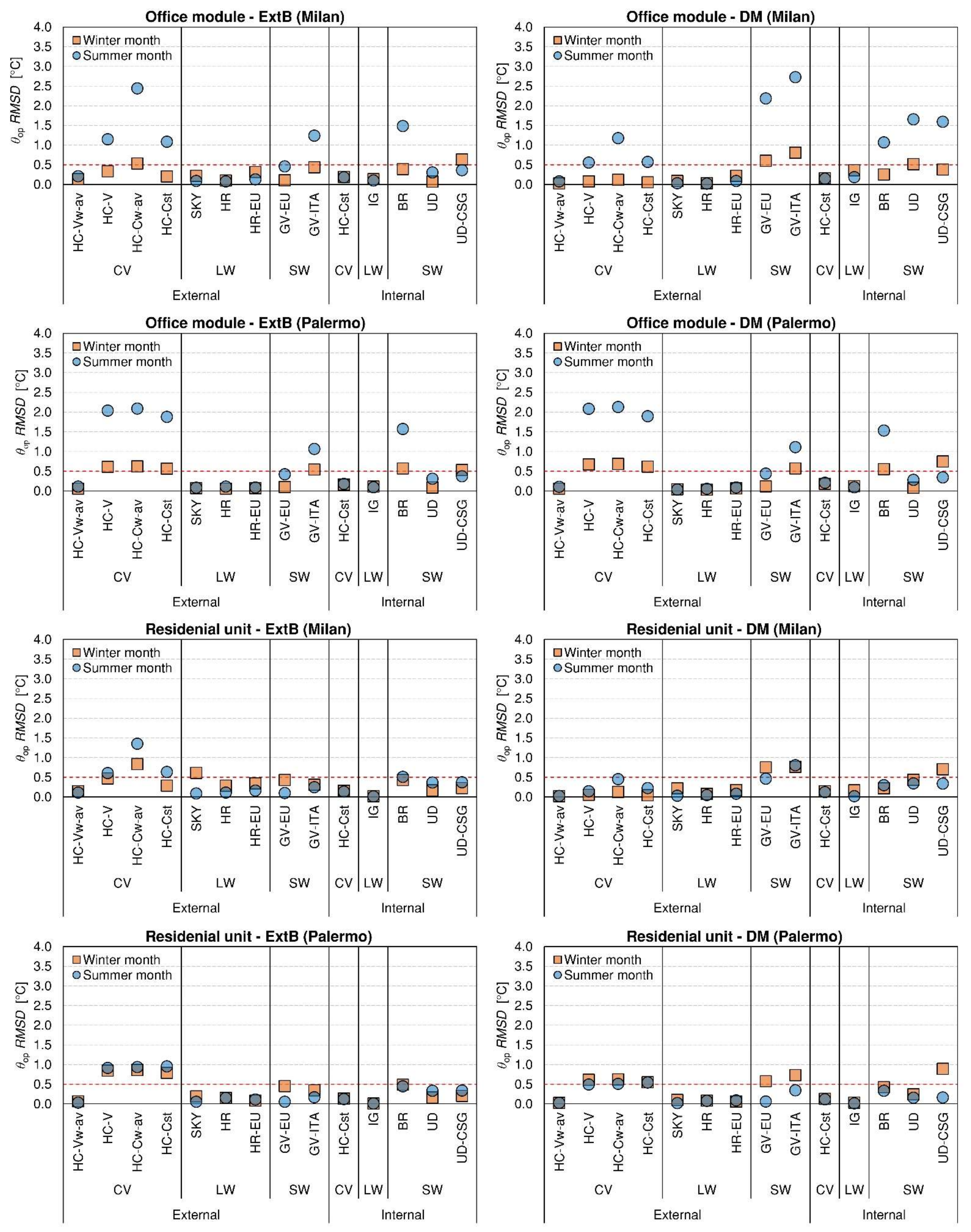
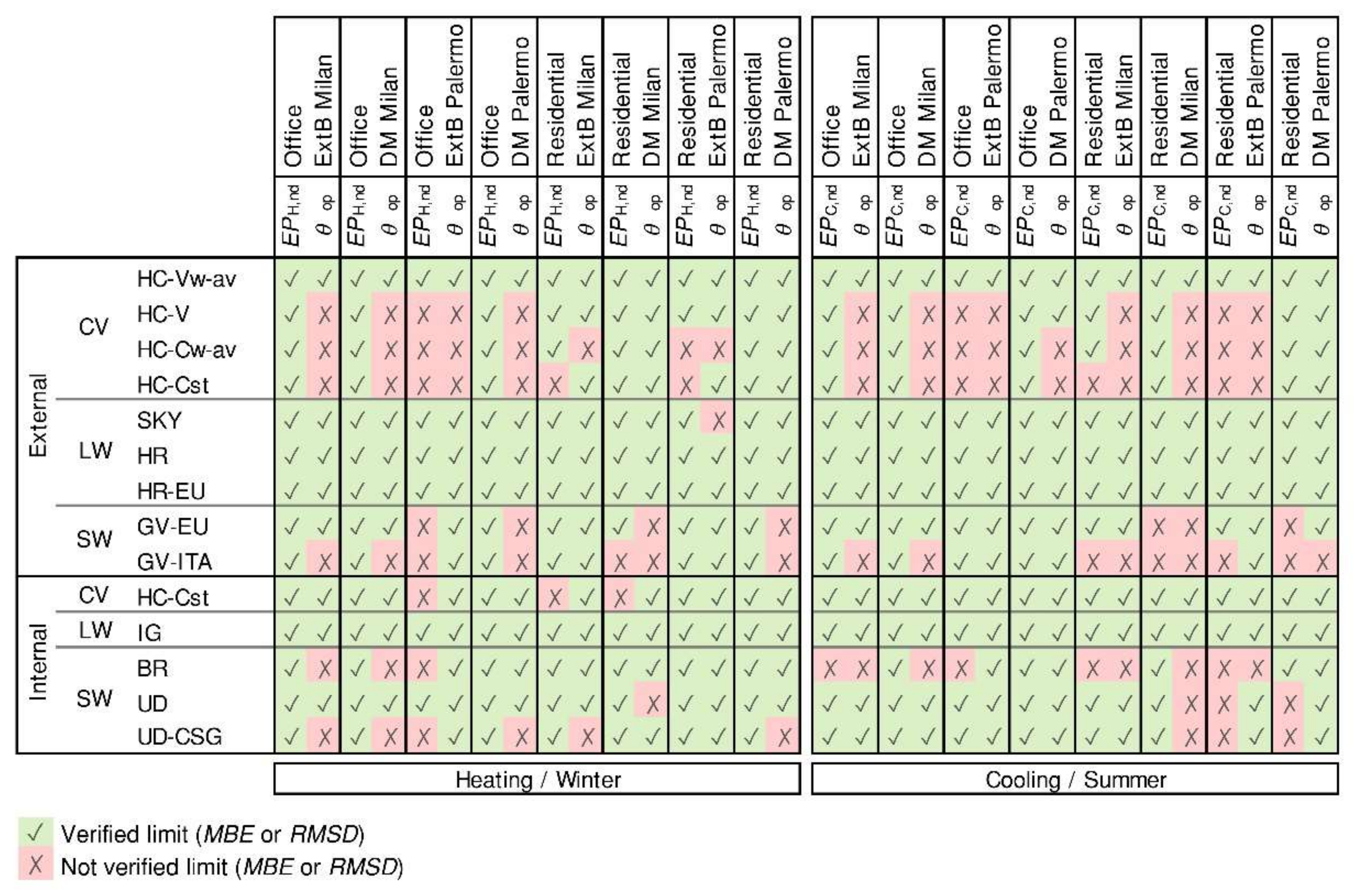
4.2. Operative Temperatures Evaluation
5. Discussion
- The simplified determination of the external convective heat transfer coefficient generally leads to inaccuracies for uninsulated buildings. In well-insulated buildings, instead, good agreements can be obtained for annual energy performance evaluations, while significant errors are committed in the prediction of the indoor operative temperatures, especially in the warm season. Thus, the EN ISO 52016-1 simplifications on the external convection heat transfer may be applied in the design phases, or for compliance checks, for new buildings. However, for energy audits of existing buildings, or for thermal comfort evaluations, it may be preferable to use more accurate calculation models.
- The use of a constant indoor convective heat transfer coefficient may lead to inaccuracies in the estimation of the energy need for heating for uninsulated buildings, while its application in the prediction of the indoor operative temperatures can be considered.
- Inaccuracies in the temperature prediction occur when the simplification on the solar radiation entering into the zone is considered (i.e., back reflection and convective solar gains). However, generally they guarantee an acceptable accuracy in terms of energy needs estimation.
6. Conclusions
Author Contributions
Funding
Institutional Review Board Statement
Informed Consent Statement
Data Availability Statement
Conflicts of Interest
References
- European Committee for Standardization (CEN). EN ISO 13790, Energy Performance of Buildings—Calculation of Energy Use for Space Heating and Cooling; CEN: Brussels, Belgium, 2007. [Google Scholar]
- European Committee for Standardization (CEN). EN ISO 52016-1, Energy Performance of Buildings—Energy Needs for Heating and Cooling, Internal Temperatures and Sensible and Latent Heat Loads—Part 1: Calculation Procedures; CEN: Brussels, Belgium, 2016. [Google Scholar]
- van Dijk, D. EN ISO 52016 1: The new International Standard to calculate building energy needs for heating and cooling, internal temperature and heating and cooling loads. In Proceedings of the Building Simulation 2019: 16th Conference of IBPSA, Rome, Italy, 2–4 September 2019; pp. 4061–4068. [Google Scholar]
- Judkoff, R.; Wortman, D.; O’Doherty, B.; Burch, J. A Methodology for Validating Building Energy Analysis Simulations; Technical Report NREL/TP-550-42059; National Renewable Energy Laboratory: Golden, CO, USA, 2008.
- Bloomfield, D.P. An overview of validation methods for energy and environmental software. In ASHRAE Transactions: Symposia; American Society of Heating, Refrigerating and Air-Conditioning Engineers: Seattle, WA, USA, 1999; Volume 105, pp. 685–693. [Google Scholar]
- Beausoleil-Morrison, I.; Griffith, B.; Vesanen, T.; Weber, A. A demonstration of the effectiveness of inter-program comparative testing for diagnosing and repairing solution and coding errors in building simulation programs. J. Build. Perform. Simul. 2009, 2, 63–73. [Google Scholar] [CrossRef]
- Buonomano, A. Code-to-Code Validation and Application of a Dynamic Simulation Tool for the Building Energy Performance Analysis. Energies 2016, 9, 301. [Google Scholar] [CrossRef] [Green Version]
- Beausoleil-Morrison, I. Inter-model comparison of embedded-tube radiant floor models in BPS tools. J. Build. Perform. Simul. 2016, 9, 190–209. [Google Scholar]
- Raslan, R.; Davies, M. Results variability in accredited building energy performance compliance demonstration software in the UK: An inter-model comparative study. J. Build. Perform. Simul. 2010, 3, 63–85. [Google Scholar] [CrossRef]
- Bloomfield, D. Appraisal techniques for methods of calculating the thermal performance of buildings. Build. Serv. Eng. Technol. 1985, 6, 13–20. [Google Scholar] [CrossRef]
- Ballarini, I.; Costantino, A.; Fabrizio, E.; Corrado, V. A Methodology to Investigate the Deviations between Simple and Detailed Dynamic Methods for the Building Energy Performance Assessment. Energies 2020, 13, 6217. [Google Scholar] [CrossRef]
- Zakula, T.; Bagaric, M.; Ferdelji, N.; Milovanovic, B.; Mudrinic, S.; Ritosa, K. Comparison of dynamic simulations and the ISO 52016 standard for the assessment of building energy performance. App. Energy 2019, 254, 113553. [Google Scholar] [CrossRef]
- Neymark, J.; Kummert, M.; Judkoff, R. Developing Equivalent Surface Heat Transfer Input Parameters for Updated Standard 140/BESTEST Thermal Fabric Test Cases. In Proceedings of the Building Simulation 2019: 16th Conference of IBPSA, Rome, Italy, 2–4 September 2019; pp. 4570–4577. [Google Scholar]
- Judkoff, R. Validation of Building Energy Analysis simulation programs at the solar energy research institute. Energy Build. 1998, 10, 221–239. [Google Scholar] [CrossRef]
- Jensen, S.O. Validation of building energy simulation programs: A methodology. Energy Build. 1995, 22, 133–144. [Google Scholar] [CrossRef]
- American Society for Heating Refrigerating Air-conditioning Engineers (ASHRAE). Guideline 14—Measurement of Energy, Demand, and Water Savings; ASHRAE: Atlanta, GA, USA, 2014. [Google Scholar]
- Zakula, T.; Badun, N.; Ferdelji, N.; Ugrina, I. Framework for the ISO 52016 standard accuracy prediction based on the in-depth sensitivity analysis. Appl. Energy 2021, 298, 117089. [Google Scholar] [CrossRef]
- Kamaraj, S.V. Dynamic Building Modelling Using an Extensive RC Network according to ISO 52016: Numerical Implementation and Testing. Ph.D. Thesis, Politecnico di Milano, Milan, Italy, 2008. [Google Scholar]
- Judkoff, R.; Wortman, D.; O’Doherty, B.; Burch, J. Building Energy Simulation Test (BESTEST) and Diagnostic Method; National Renewable Energy Laboratory: Golden, CO, USA, 1998.
- Ballarini, I.; Costantino, A.; Fabrizio, E.; Corrado, V. The dynamic model of EN ISO 52016-1 for the energy assessment of buildings compared to simplified and detailed simulation methods. In Proceedings of the Building Simulation 2019: 16th Conference of IBPSA, Rome, Italy, 2–4 September 2019; pp. 3847–3854. [Google Scholar]
- Mazzarella, L.; Scoccia, R.; Colombo, P.; Motta, M. Improvement of EN ISO 52016-1:2017 hourly heat transfer thought a wall assessment: The Italian National Annex. Energy Build. 2020, 210, 109758. [Google Scholar] [CrossRef]
- De Luca, G.; Bianco Mauthe Degerfeld, F.; Ballarini, I.; Corrado, V. The Effect of the External Driving Forces Modelling on the Calculated Building Energy Need Through the Use of Dynamic Simulation. In Proceedings of the Building Simulation 2021: 17th Conference of IBPSA, Bruges, Belgium, 1–3 September 2021. in press. [Google Scholar]
- European Committee for Standardization (CEN). EN ISO 6946, Building Components and Building Elements—Thermal Resistance and Thermal Transmittance—Calculation Methods; CEN: Brussels, Belgium, 2017. [Google Scholar]
- Walton, G.N.; National Bureau of Standards. Thermal Analysis Research Program Reference Manual. NBSSIR 83-2655; U.S. Department of Commerce: Washington, DC, USA, 1983. [Google Scholar]
- Sparrow, E.M.; Ramsey, J.W.; Mass, E.A. Effect of Finite Width on Heat Transfer and Fluid Flow about an Inclined Rectangular Plate. J. Heat Transf. 1979, 101, 204. [Google Scholar] [CrossRef]
- Evangelisti, L.; Guattari, C.; Asdrubali, F. On the sky temperature models and their influence on buildings energy performance: A critical review. Energy Build. 2019, 183, 607–625. [Google Scholar] [CrossRef]
- Clark, G.; Allen, C. The Estimation of Atmospheric Radiation for Clear and Cloudy Skies. In Proceedings of the 2nd National Passive Solar Conference, Philadelphia, PA, USA, 16–18 March 1978. [Google Scholar]
- Karlsson, J.; Roos, A. Modelling the angular behaviour of the total solar energy transmittance of windows. Sol. Energy 2000, 69, 312–329. [Google Scholar] [CrossRef]
- European Committee for Standardization (CEN). EN ISO 13789, Thermal Performance of Buildings—Transmission and Ventilation Heat Transfer Coefficients—Calculation Method; CEN: Brussels, Belgium, 2017. [Google Scholar]
- U.S. Department of Energy. EnergyPlus™ Version 9.4.0 Documentation: Engineering Reference; National Renewable Energy Laboratory: Golden, CO, USA, 2020.
- European Committee for Standardization (CEN). EN ISO 52017, Energy Performance of Buildings—Sensible and Latent Heat Loads and Internal Temperatures—Part 1: Generic Calculation Procedures; CEN: Brussels, Belgium, 2017. [Google Scholar]
- European Committee for Standardization (CEN). EN ISO 13791, Thermal Performance of Buildings—Calculation of Internal Temperatures of a Room in Summer without Mechanical Cooling—General Criteria and Validation Procedures; CEN: Brussels, Belgium, 2012. [Google Scholar]
- pyEp 0.9.4.4. Available online: https://pypi.org/project/pyEp/ (accessed on 10 July 2021).
- Italian Republic. Inter-Ministerial Decree of 26 June 2015, Applicazione delle Metodologie di Calcolo delle Prestazioni Energetiche e Definizione delle Prescrizioni e dei Requisiti Minimi Degli Edifici. Off. J. Ital. Repub. 2015, 162, 39. [Google Scholar]
- Loga, T.; Diefenbach, N.; Stein, B. Typology Approach for Building Stock Energy Assessment. Main Results of the TABULA Project; Institut Wohnen und Umwelt GmbH: Darmstadt, Germany, 2012. [Google Scholar]
- Italian Ministry of the Economic Development and Ministry of the Environment. Updating of the Italian Application of the Cost-Optimal Calculation Methodology for the Minimum Energy Performance Requirements (Directive 2010/31/EU Art. 5); Italian Ministry of the Economic Development and Ministry of the Environment: Rome, Italy, 2018.
- Italian Organisation for Standardisation (UNI). UNI/TR 11552, Opaque Envelope Components of Buildings—Thermo-Physical Parameters; UNI: Rome, Italy, 2014. [Google Scholar]
- Italian Organisation for Standardisation (UNI). UNI 10349-3, Heating and Cooling of Buildings—Climatic Data—Part 3: Accumulated Temperature Differences (Degree-Days) and Other Indices; UNI: Rome, Italy, 2016. [Google Scholar]
- European Committee for Standardization (CEN). EN 16798-1, Energy Performance of Buildings—Ventilation for Buildings—Part 1: Indoor Environmental Input Parameters for Design and Assessment of Energy Performance of Buildings Addressing Indoor Air Quality, Thermal Environment, Lighting and Acoustics—Module M1-6; CEN: Brussels, Belgium, 2019. [Google Scholar]
- EnergyPlus Weather Data Sources. Available online: https://energyplus.net/weather/sources (accessed on 10 July 2021).
- EnergyPlus. Available online: https://energyplus.net/ (accessed on 10 July 2021).


| Parameters | Residential Apartment-Unit | Office Module |
|---|---|---|
| Conditioned net floor area, An | 66.3 m2 | 17.8 m2 |
| Conditioned net volume, Vn | 179.0 m3 | 48.1 m3 |
| Transparent area (vs. external), Aenv,w | 9.1 m2 | 4.8 m2 |
| Opaque area (vs. external), Aenv,op | 52.7 m2 | 5.5 m2 |
| Compactness ratio, S/V | 0.35 m−1 | 0.21 m−1 |
| Windows-to-wall ratio, WWR | 0.34 (South wall) | 0.47 (West wall) |
| 0.00 (West wall) | ||
| 0.27 (North wall) |
| Envelope Component | Milan (Climatic Zone E) 1 | Palermo (Climatic Zone B) 2 |
|---|---|---|
| External wall (Uwall,DM) | 0.26 W·m−2·K−1 | 0.43 W·m−2·K−1 |
| Windows (Uwin,DM) | 1.4 W·m−2·K−1 (g = 0.50) | 3.0 W·m−2·K−1 (g = 0.75) |
Publisher’s Note: MDPI stays neutral with regard to jurisdictional claims in published maps and institutional affiliations. |
© 2021 by the authors. Licensee MDPI, Basel, Switzerland. This article is an open access article distributed under the terms and conditions of the Creative Commons Attribution (CC BY) license (https://creativecommons.org/licenses/by/4.0/).
Share and Cite
De Luca, G.; Bianco Mauthe Degerfeld, F.; Ballarini, I.; Corrado, V. Accuracy of Simplified Modelling Assumptions on External and Internal Driving Forces in the Building Energy Performance Simulation. Energies 2021, 14, 6841. https://0-doi-org.brum.beds.ac.uk/10.3390/en14206841
De Luca G, Bianco Mauthe Degerfeld F, Ballarini I, Corrado V. Accuracy of Simplified Modelling Assumptions on External and Internal Driving Forces in the Building Energy Performance Simulation. Energies. 2021; 14(20):6841. https://0-doi-org.brum.beds.ac.uk/10.3390/en14206841
Chicago/Turabian StyleDe Luca, Giovanna, Franz Bianco Mauthe Degerfeld, Ilaria Ballarini, and Vincenzo Corrado. 2021. "Accuracy of Simplified Modelling Assumptions on External and Internal Driving Forces in the Building Energy Performance Simulation" Energies 14, no. 20: 6841. https://0-doi-org.brum.beds.ac.uk/10.3390/en14206841