Pumping Schedule Optimization in Acid Fracturing Treatment by Unified Fracture Design

Abstract

Acid fracturing simulation has been widely used to improve well performance in carbonate reservoirs. In this study, a computational method is presented to optimize acid fracturing treatments. First, fracture geometry parameters are calculated using unified fracture design methods. Then, the controllable design parameters are iterated till the fracture geometry parameters reach their optimal values. The results show higher flow rates are required to achieve optimal fracture geometry parameters with larger acid volumes. Detailed sensitivity analyses are performed on controllable and reservoir parameters. It shows that higher flow rates should be applied for fluids with lower viscosity. Straight acid reaches optimal conditions at higher flow rates and lower volumes. These conditions for retarded acids appear to be only at lower flow rates and higher volumes. The study of the acid concentration for gelled acids shows that both flow rate and volume increase as the concentration increases. For the formation with lower permeability, a higher flow rate is required to achieve the desired larger fracture half-length and smaller fracture width. Further investigations also show that the formation with higher Young’s modulus requires decreasing the acid volume and increasing the optimal flow rate, while the formation with higher closure stress requires increasing the acid volume and decreasing the flow rate.

1. Introduction

Acid fracturing treatment has been widely used to improve well performance in carbonate reservoirs. The first stage of the acid fracturing treatment creates an initial fracture by applying pressure higher than the formation breakdown pressure. At this stage, a non-reactive fluid called a pad is injected. In order to facilitate rock dissolution on the fracture walls created by the pad, acid is injected into the well. At the end of the treatment, the pressure is released, and the fracture is allowed to close by the in situ stress. Due to the removal of the rock at the fracture walls, the fracture, however, does not close entirely, which improves the hydraulic connection of the well to the reservoir.

In the past few decades, extensive studies were conducted on the acid fracturing process, emphasizing acid-induced dissolution and acid-etched width. An acid transport equation for the one-dimensional steady-state is presented in [1,2]. Additionally, a method was established to describe the matrix acidizing, considering all the variables [3]. Schechter assumed that all flow entering between the plates leaks out of the channel uniformly and calculated velocity profiles with Berman’s method [4,5]. A leak-off model that includes the wormhole’s effect on the acid fracturing was presented in [6]. In this model, overall fluid leak-off is controlled by three mechanisms. These mechanisms include reservoir fluid compressibility, the thickness of the invaded zone, and filter cake formed on the fracture wall. A fracture acidizing simulator method that considered the effect of the parameters such as fracture geometry, temperature, and acid spending process was developed in [7]. Navarrete investigated the effect of acid retardation on the resulting acid-etched width [8].

In order to achieve realistic results and minimize the limitations of analytical methods, numerical methods have also been developed. Lo and Dean calculated the two-dimensional diffusion–convection equation by considering an average for acid concentration along the fracture width [9]. Settari et al. developed a two-dimensional model of acid transport in the unsteady state by considering the flow influence in two directions of length and width and minor changes in the direction of fracture height [10]. Romero et al. developed a model to eliminate the effect of mass transfer coefficient on the calculation of acid transported to the fracture walls [11]. They considered the influence of the acid transfer in the direction of the fracture walls. A fully three-dimensional model using the SIMPLEM algorithm proposed by Mou et al. [12]. They calculated the 3D velocity fields for an intermediate-scale acid fracture model and simulated the acid transport process within a random region of the acid fracturing. The Mou method [12] was modified for acid fracturing treatments at the field scale [13]. The effects of the three types of acid systems on fracture conductivity and acid penetration distance was investigated in [14]. Alhubail et al. developed an acid transport model using the finite element method to improve treatment efficiency [15]. Ugursal et al. presented a new model for predicting acid fracturing performance in naturally fractured carbonate reservoirs and investigated the effect of natural fractures on acid fracturing stimulation efficiency [16]. Acid filtration in a fractured reservoir to investigate acid filtration in natural fractures, wormholes, and matrix on acid injection distance was modeled [17].

An important issue that can reduce the cost and risk of acid fracturing treatment is acid fracturing optimization. A model coupling fracture geometry to the diffusion mechanism was presented in [18]. Guo et al. researched three-dimensional modeling of acid fracturing and optimization design, and proposed a technique for achieving the maximum net present value [19]. A method was used to estimate the optimal length and conductivity using the UFD approach [20]. Ai et al. coupled the fracture geometry optimization with treatment parameter optimization to maximize the dimensionless productivity index [21]. A comprehensive acid fracturing model to optimize design parameters was used [22,23]. Aljawad et al. proposed a method to investigate the impact of diversion on acid fracturing of laminated carbonate formations [24]. Al-Ameri et al. employed FRACPRO software to optimize acid fracturing design for a tight carbonate reservoir to investigate the impact of acid injection stages and acid fluids types on the fracture geometry parameters and the fracture conductivity [25]. A simple and computationally efficient model are used for evaluating acid fracturing efficiency in naturally fractured reservoirs using artificial intelligence-based techniques [26].

Pumping schedule optimization with all these methods requires desirable conditions to be selected manually between several options. The primary purpose of this paper is to minimize the risk of the acid fracturing treatment. Therefore, some iterative simulations were performed for optimization of the fracture geometry parameters using the UFD approach. Therefore, design parameters were changed to each specified optimization goal. In the following, first, the methodology for optimization fracture geometry parameters is described. Then, the parametric study is implemented to investigate the influence of the formation’s inherent properties and controllable parameters on the optimal rate and volume. Finally, the main results of this study are presented.

2. Methods

2.1. Workflow

Figure 1 illustrates the workflow of the proposed method. First, the initial data listed in

Table 1. Data required by the proposed method.

Parameter	Value	Unit
Formation properties
Young’s Modulus (E)	6	MMPsi
Poisson Ratio ($\upsilon$)	0.25	-
Porosity ($\varnothing$)	0.071	-
Permeability (k)	0.4	md
Wormhole breakthrough pore volume ($Q_{ibt}$)	1.5	-
Layer Thickness (H)	50	m
Closure Stress (${\sigma }_c$)	4200	Psi
Total compressibility ($C_t$)	1.983 × 10−5	${\mathrm{Psi}}^{-1}$
Reservoir Oil Viscosity (${\mu }_{Oil}$)	1.66	cp
Formation Rock Density (${\rho }_{Rock}$)	2600	$\mathrm{kg}/{\mathrm{m}}^3$
Reservoir Temperature (T)	246	°F
Reservoir Pressure ($p_r$)	3000	Psi
Fracturing Pressure ($p_f$)	4300	Psi
Acid Properties
Density (${\rho }_{Acid}$)	1000	$\mathrm{kg}/{\mathrm{m}}^3$
Acid initial concentration ($c_i$)	4.4 (16%)	$\mathrm{moles}/{\mathrm{dm}}^3$
Spurt loss ($S_p$)	0	m
Fraction of acid to react before leaking off ($f_r$)	0.3	-
Reaction order ($n^{\prime }$)	0.63	-
Reaction rate coefficient ($E_f$)	0.3263	$\frac{\mathrm{kg} \mathrm{moles} \mathrm{HCl}}{{\mathrm{m}}^2\mathrm{s}{\left(\frac{\mathrm{kg} \mathrm{moles} \mathrm{HCl}}{{\mathrm{m}}^3 \mathrm{acid} \mathrm{solution}}\right)}^{\mathrm{n}\prime }}$
Parameters of UFD method
Volumetric dissolving power ($\mathcal{X}$)	0.082	-
Drainage radius ($r_e$)	1900	Ft
Dimensionless horizontal correlation length (${\lambda }_{D,x}$)	1	-
Dimensionless vertical correlation length (${\lambda }_{D,Z}$)	0.05	-
Dimensionless standard deviation of permeability (${\sigma }_D$)	0.4	-

are entered into the model. Data include formation and rock properties, acid properties, and parameters of the UFD method. Then, optimal fracture geometry parameters for a specific volume are calculated using the UFD method. In the next step, an initial guess for the injected flow rate is made. After that, the flow rate is iterated to achieve the optimal fracture geometry parameters. As reported in previous studies, the fracture propagation and acid transport models are simulated for a specific flow rate [13,27]. The details of the fracture propagation and acid transport models are given in Section 2.3 and Section 2.4, respectively. The condition of convergence is to minimize the Equation (1). It should be noted that an optimal flow rate is estimated for any specific acid volume. This process continues until the final acid volume is reached.

$$Error=\sqrt{{\left(\frac{x_f}{x_{Opt}}-1\right)}^2+{\left(\frac{{\overline{w}}_{Acid}}{w_{Opt}}-1\right)}^2}$$

(1)

where $x_f$ is estimated fracture half-length for a specific flow rate, $x_{Opt}$ is optimal fracture half-length, ${\overline{w}}_{Acid}$ is estimated average acid-etched width for a specific flow rate and $w_{Opt}$ is the optimal fracture width.

2.2. Optimization of the Fracture Geometry Parameters

The UFD method expresses the analytical solution for the optimal dimensionless fracture conductivity to maximize the dimensionless productivity index, given a volume of acid. As a result, optimal acid fracture parameters are obtained during the following steps:

• For a specific acid volume and an initial guess for final $x_{Opt}$ ($x_{Old}$), the average ideal fracture width is as [4]:

  $$\overline{w_i}=\frac{\mathcal{X}{V}_{acid}}{2\left(1-\varnothing \right)x_{Old}{h}_f}$$

  (2)

  where $\varnothing$ is porosity, $x_{Old}$ is initial guess optimal fracture half-length, $h_f$ is the fracture height and is equal to the net pay of the formation. $V_{acid}$ is injected acid volume, and $\mathcal{X}$ is volumetric dissolving power.
• One of the important parameters to estimate the fracture conductivity is the average ideal fracture width. A geostatistical method was employed to calculate the fracture conductivity [28] (Equation (3)). In this method, the effect of the spatial behavior of the formation’s permeability and elastic properties are considered in the calculations. Since the fracture conductivity is approximately proportional to ${\overline{w_i}}^{2.5}$, it is important, therefore, that the acid-etched width be accurately determined [29].

  $$\begin{array}{c}{k}_f=C_1\exp \left(-C_2{\sigma }_c\right)\\ C_1=4.48\times {10}^9\left[0.1756{\left(erf\left(0.8{\sigma }_D\right)\right)}^3{\overline{w_i}}^{2.49}\right]\times [1+(1.82erf(3.25({\lambda }_{D,x}-\\ 0.12\left)\right)-1.31erf\left(6.71\left({\lambda }_{D,z}-0.03\right)\right)\left)\sqrt{exp\left({\sigma }_D\right)-1}\right]\times [0.22{\left({\lambda }_{D,x}{\sigma }_D\right)}^{2.8}+\\ {0.01{\left(\left(1-{\lambda }_{D,z}\right){\sigma }_D\right)}^{0.4}]}^{0.52}\\ C_2=[14.9-3.78ln\left({\sigma }_D\right)-6.81ln\left(E\right)]\times {10}^{-4}\end{array}$$

  (3)

  where ${\lambda }_{D,x}$ is the dimensionless horizontal correlation length, ${\lambda }_{D,z}$ is the dimensionless vertical correlation length, and ${\sigma }_D$ is the dimensionless standard deviation of permeability. ${\sigma }_c$ is closure stress, $E$ is Young’s modulus, and $\overline{w_i}$ is the calculated average ideal fracture width in the previous step. $C_1$ and $C_2$ are constant coefficients and erf refers to the error function that is given in the model.
• After that, the proppant number for acid fracturing is determined, as reported in [30]. An equivalent proppant number was used for calculating the optimum dimensionless fracture conductivity.

  $$N_A=\frac{2k_f{V}_f}{k{V}_r}$$

  (4)

  $$C_{FD\text{\_}Opt}=\{\begin{array}{cc}1.6& N_A<0.1\\ 1.6+exp\left[\frac{-0.583+1.48Ln\left(N_A\right)}{1+0.142Ln\left(N_A\right)}\right]& 0.1\le N_A\le 10\\ 1.6& N_A>10\end{array}$$

  (5)
• In this step, the optimal fracture half-length and optimal fracture width are calculated as in [30]:

  $$x_{Opt}={\left(\frac{k_f{V}_f}{2C_{FD\text{\_}Opt}k{h}_f}\right)}^{0.5}$$

  (6)

  $$w_{Opt}={\left(\frac{C_{FD\text{\_}Opt}k{V}_f}{2k_f{h}_f}\right)}^{0.5}$$

  (7)
• Finally, the calculated fracture half-length and fracture width from Equations (6) and (7) are compared with initial $x_{Old}$ and $\overline{w_i}$. This process continues until the estimated values reach a stable condition.

2.3. Fracture Propagation Model

During acid fracturing, the fracture’s initial geometry is formed by a mechanical process similar to proppant fracturing. The geometry of the fracturing propagation model is based on the PKN method, and fracture half-length is determined as follows [27]:

$$x_f=\frac{q\left(\overline{w}+2S_p\right)}{4\pi h_f{C}_L{}^2}\left[\exp \left({\overline{\beta }}^2\right)erfc\left(\overline{\beta }\right)+\frac{2\overline{\beta }}{\pi }-1\right],\overline{\beta }=\frac{2C_L\sqrt{\pi t}}{\overline{w}+2S_p}$$

(8)

where $q$ is the injected flow rate, $S_p$ is spurt loss coefficient, $\overline{\beta }$ is a constant parameter, $h_f$ is fracture height, $C_L$ is the leak-off coefficient, $t$ is the injection time, and $\overline{w}$ is the averaged fracture width in the pad stage that can be calculated as:

Newtonian:

$$\overline{w}=2.05{\left(\frac{\left(1-{\upsilon }^2\right)\mu q{x}_f}{E}\right)}^{0.25}$$

(9)

Non-Newtonian:

$$\overline{w}=\frac{\pi }{5}{9.15}^{\left(\frac{1}{2n+2}\right)}{3.98}^{\left(\frac{n}{2n+2}\right)}{\left[\frac{1+2.14n}{n}\right]}^{\left(\frac{n}{2n+2}\right)}{K}^{\left(\frac{1}{2n+2}\right)}{\left[\frac{\left(1-{\upsilon }^2\right)x_f{q}^n{h}_f{}^{\left(1-n\right)}}{E}\right]}^{\left(\frac{1}{2n+2}\right)}$$

(10)

where $\mu$ is fracture-fluid viscosity, $\upsilon$ is the Poisson ratio, $E$ is the Young’s modulus, $n$ is power in the power-law model, and $K$ is the consistency index. Additionally, fracture half-length, averaged fracture width, maximum width, and net pressure are calculated by numerical root-finding methods [27].

2.4. Acid Model

During acid injection, the fracture width (Figure 2) changes continuously as the rock dissolves. In the acid model, the length and height of the fracture are fixed. At each time step, the fracture propagation model provides the domain for the acid solution. The boundary and initial conditions are applied. At the next step, the finite difference method is employed to solve the velocity and pressure components within the fracture. Then, the flow rate is estimated in the fracture entrance. If the estimated flow rate is equal to initial flow rate, then acid concentration is calculated, otherwise fluid pressure must be set. The acid etched width can now be obtained. At the end of treatment time, fracture conductivity within the fracture domain is estimated.

2.4.1. Fluid Velocity Components and Pressure

In order to estimate acid concentration within the fracture, the fluid velocity components should be calculated. Navier–Stokes equations are used for this purpose. The closed-form of the momentum equation is as following:

$$\rho \left\{\frac{\partial v_i}{\partial t}+v_j\frac{\partial v_i}{\partial x_j}\right\}+\frac{\partial p}{\partial x_i}=\mu \frac{{\partial }^2{v}_i}{\partial x_j\partial x_j}$$

(11)

The continuity equation of fluid flows is obtained according to:

$$\frac{\partial v_i}{\partial x_i}=0$$

(12)

where $\rho$ is the fluid density, $p$ is the fluid net pressure, $\mu$ is the fracture-fluid viscosity, and $v_i$ is the velocity vector. The geometry created by the acid fracturing has an irregular shape, but the Equations (11) and (12) can be used for regular shapes. Therefore, the Crank method can be used [31]. As reported in previous studies, the FDM method [32] and SIMPLEM algorithm [33] are employed to solve the velocity and fluid net pressure components within the fracture. Net pressure means the difference in pressure between fracture propagation pressure and closure stress.

2.4.2. Calculate the Acid Concentration

The acid concentration profile gives the amount of acid that reaches the surfaces. Acid due to convection and diffusion are transformed to the fracture surfaces, so we consider diffusion and convection in the $x$-direction. Diffusion in the $x$ and $z$ directions is neglected because convection dominates the acid flow in these directions [12]. The mass continuity equation is used to calculate the acid concentration profile within the fracture.

$$\frac{\partial C_D}{\partial t}+u\frac{\partial C_D}{\partial x}+v\frac{\partial C_D}{\partial y}+w\frac{\partial C_D}{\partial z}=\frac{\partial }{\partial y}\left(D_{eff}\frac{\partial C_D}{\partial y}\right)$$

(13)

where $D_{eff}$ is effective acid diffusion coefficient and $C_D$ is the dimensionless acid concentration that changes over time along fracture length, height, and width.

2.4.3. Rocks Displacement on the Fracture Surfaces

The amount of rock dissolution can be obtained by calculating the acid concentration profile. Acid leak-off and a gravity force gradient transport acid to the walls. The acid-etched width can be calculated as follows [32]:

$$\frac{\partial y}{\partial t}=\frac{\beta M{W}_{acid}{C}_i}{{\rho }_{rock}\left(1-\varnothing \right)}\left(f_r{v}_L{C}_D-D_{eff}\frac{\partial C_D}{\partial y}\right)$$

(14)

where ${\rho }_{rock}$ is formation rock density, $\varnothing$ is porosity, $v_L$ is leak-off velocity, $C_i$ is injected acid concentration. The type of acid may change with changing gravitational dissolving power ($\beta$) and the acid’s molecular weight ($M{W}_{acid}$). Part of the acid reacts with the walls before leak-off into the formation; this parameter is expressed by $f_r$.

2.4.4. Boundary Condition

The velocity boundary conditions at the top and bottom of the fracture are such that no slippage occurs.

$${u|}_{z=0,H}={v|}_{z=0,H}={w|}_{z=0,H}=0$$

(15)

The fluid velocity at the entrance and end of the fracture in both $y$ and $z$ directions is such that no slippage occurs.

$${v|}_{x=0,L}={w|}_{x=0,L}=0$$

(16)

At the entrance of the fracture, the fluid flows only in the direction of the $x$-axis. The boundary conditions are a function of the injection flow rate and the flow entrance cross-section.

$$q=\underset{0}{\overset{h_f}{{\displaystyle \int }}}\mathrm{dz}\underset{\raisebox{1ex}{$-b$}\!\left/ \!\raisebox{-1ex}{$2$}\right.}{\overset{\raisebox{1ex}{$b$}\!\left/ \!\raisebox{-1ex}{$2$}\right.}{{\displaystyle \int }}}{u|}_{x=0}dy$$

(17)

Fluid velocity boundary conditions in the fracture surfaces are presented as follows:

$$\begin{array}{c}{u|}_{y=\raisebox{1ex}{$-b$}\!\left/ \!\raisebox{-1ex}{$2$}\right.,\raisebox{1ex}{$b$}\!\left/ \!\raisebox{-1ex}{$2$}\right.}={w|}_{y=\raisebox{1ex}{$-b$}\!\left/ \!\raisebox{-1ex}{$2$}\right.,\raisebox{1ex}{$b$}\!\left/ \!\raisebox{-1ex}{$2$}\right.}=0\\ {v|}_{y=\raisebox{1ex}{$-b$}\!\left/ \!\raisebox{-1ex}{$2$}\right.,\raisebox{1ex}{$b$}\!\left/ \!\raisebox{-1ex}{$2$}\right.}=v_L\left(t\right)\end{array}$$

(18)

The fluid velocity component in both $x$ and $z$ directions on the fracture surfaces (⁻$\raisebox{1ex}{$b$}\!\left/ \!\raisebox{-1ex}{$2$}\right.$ and $\raisebox{1ex}{$b$}\!\left/ \!\raisebox{-1ex}{$2$}\right.$) is zero. The fluid velocity component along the $y$ axis located in the fracture surfaces is based on fluid leak-off velocity changes [34]. The leak-off rate depends on a leak-off coefficient and is proportional to the treatment time’s root inverse [6].

$$v_L\left(t\right)=\frac{C_L}{\sqrt{t-t_0}}$$

(19)

where $C_L$ is the leak-off coefficient and estimated by the method as present in the next step [6].The exposure time $t-t_0$ at a particular location on the fracture is the time elapsed between the current time $t$ and $t_0$ at which the fracture tip arrived at that location. The initial concentration of acid is zero everywhere in the fracture.

$${C|}_{t=0}=0$$

(20)

The acid concentration at the fracture inlet is equal to the initial amount of acid.

$${C|}_{x=0}=C_i$$

(21)

The acid reaction at fracture surfaces is a function of acid concentration [1,35]. The boundary conditions of the acid concentration are applied on the fracture surfaces as:

$$D_{eff}{C}_i\frac{\partial C_D}{\partial y}=E_f{\left(C_i{C}_D-C_{eqm}\right)}^{n^{\prime }}\left(1-\varnothing \right)$$

(22)

where $E_f$ is reaction rate coefficient, $n^{\prime }$ is reaction order, and $C_{eqm}$ is acid equilibrium concentration. The acid reaction at the top and bottom of the fracture is zero.

$$\frac{\partial C_D}{\partial z}=0$$

(23)

2.5. Leak-Off Model

The leak-off coefficient is a critical parameter [18]. The shape of the fracture and the penetration distance are both affected by this value. The leak-off coefficient is one of the input parameters in the developed algorithm. The leak-off coefficient is calculated as reported in previous studies [6]. The overall fluid leak-off is controlled by the filtration fluid viscosity effect ($C_v$), wall building effect ($C_w$), and reservoir fluid viscosity and compressibility effect ($C_c$). Under the assumption that $C_w$ is large when compared with $C_v$ or $C_c$, the total leak-off coefficient is calculated as [6].

$$C_L=\frac{\frac{-1}{C_c}+\sqrt{\frac{1}{C_c{}^2}+\frac{4}{C_{v,wh}{}^2}}}{\left(\frac{2}{C_{v,wh}{}^2}\right)}$$

(24)

where $C_v$ and $C_c$ could be determined from Equations (25) and (26), respectively.

$$C_v=\sqrt{\frac{\mathsf{\Delta }p\varnothing k}{2{\mu }_a}}$$

(25)

$$C_c=\mathsf{\Delta }p\sqrt{\frac{\varnothing k{c}_t}{\pi {\mu }_{Oil}}}$$

(26)

where $\mathsf{\Delta }p$ is pressure difference between fracture and formation, $\varnothing$ is rock porosity, $k$ is formation permeability, ${\mu }_{Oil}$ is the oil viscosity, $c_t$ is total compressibility, and ${\mu }_a$ is acid viscosity. The viscous fluid-loss coefficient with wormholing ($C_{v,wh}$) is related to the usual viscous fluid-loss coefficient without wormholes ($C_v$) by Equation (27).

$$C_{v,wh}=C_v\sqrt{\frac{Q_{ibt}}{Q_{ibt}-1}}$$

(27)

where, $Q_{ibt}$ is number of PV’s injected at wormhole breakthrough.

3. Results and Discussion

3.1. Acid Model Validation

The acid model was compared with the Schechter analytical method [4]. Additionally, the Terrill (1965) method was used for a specific condition to estimate dimensionless acid concentration along the fracture half-length. The convection/diffusion equation for a steady-state condition and zero acid concentration at the fracture walls can be calculated as follows [36].

$$\frac{\overline{c}}{C_i}={\displaystyle \sum }_{m=0}^{\infty }{G}_m{\left(1-\frac{x}{x_f}\right)}^{\raisebox{1ex}{$2{\lambda }_m^2$}\!\left/ \!\raisebox{-1ex}{$3N_{Pe}$}\right.}$$

(28)

where, $\overline{c}$ is mean acid concentration, $C_i$ initial acid concentration, ${\lambda }_m$ are eigenvalues, and $G_m$ are constants. The first five terms in the Equation (28) for realistic values of Reynolds number ($0.001<N_{R{e}^{\ast }}<1$) and Peclet number ($N_{Pe}<8$) are presented in a previous study, ${\lambda }_m$ and $G_m$ are calculated as follows [4].

$${\lambda }_m={\displaystyle \sum }_{i=0}^3{g}_{i,m}{(N_{Pe})}^i+{\displaystyle \sum }_{i=1}^2{h}_{i,m}{(N_{R{e}^{\ast }})}^i$$

(29)

$$G_m={\displaystyle \sum }_{i=0}^3{\overline{g}}_{i,m}{(N_{Pe})}^i+{\displaystyle \sum }_{i=1}^2{\overline{h}}_{i,m}{\left(N_{R{e}^{\ast }}\right)}^i$$

(30)

where, values $g_{i,m}$, $h_{i,m}$, ${\overline{g}}_{i,m}$, and ${\overline{h}}_{i,m}$ are given in

Table 2. Constant coefficients for Equations (29) and (30) to calculate ${\lambda }_m$ and $G_m$.

$\mathit{m}$	${\mathit{g}}_{\mathbf{0}\mathbf{,}\mathit{m}}\mathbf{\times }{\mathbf{10}}^{\mathbf{0}}$	${\mathit{g}}_{\mathbf{1}\mathbf{,}\mathit{m}}\mathbf{\times }{\mathbf{10}}^{\mathbf{-}\mathbf{1}}$	${\mathit{g}}_{\mathbf{2}\mathbf{,}\mathit{m}}\mathbf{\times }{\mathbf{10}}^{\mathbf{-}\mathbf{3}}$	${\mathit{g}}_{\mathbf{3}\mathbf{,}\mathit{m}}\mathbf{\times }{\mathbf{10}}^{\mathbf{-}\mathbf{4}}$	${\mathit{h}}_{\mathbf{1}\mathbf{,}\mathit{m}}\mathbf{\times }{\mathbf{10}}^{\mathbf{-}\mathbf{3}}$	${\mathit{h}}_{\mathbf{2}\mathbf{,}\mathit{m}}\mathbf{\times }{\mathbf{10}}^{\mathbf{-}\mathbf{3}}$
0	1.68231	−2.26693	6.7544	−1.8408	6.7593	−4.6274
1	5.67053	−0.696	17.2931	−2.9304	1.0032	−3.4376
2	9.66842	−0.39587	10.7745	−0.5564	−5.7028	−0.4705
3	13.66772	−0.27662	7.9375	−0.1358	−9.15	−0.5668
4	17.6674	−0.21305	6.34331	−0.0373	−12.4496	−0.71196
$\mathit{m}$	${\overline{\mathit{g}}}_{\mathbf{0}\mathbf{,}\mathit{m}}\mathbf{\times }{\mathbf{10}}^{\mathbf{-}\mathbf{1}}$	${\overline{\mathit{g}}}_{\mathbf{1}\mathbf{,}\mathit{m}}\mathbf{\times }{\mathbf{10}}^{\mathbf{-}\mathbf{4}}$	${\overline{\mathit{g}}}_{\mathbf{2}\mathbf{,}\mathit{m}}\mathbf{\times }{\mathbf{10}}^{\mathbf{-}\mathbf{4}}$	${\overline{\mathit{g}}}_{\mathbf{3}\mathbf{,}\mathit{m}}\mathbf{\times }{\mathbf{10}}^{\mathbf{-}\mathbf{5}}$	${\overline{\mathit{h}}}_{\mathbf{1}\mathbf{,}\mathit{m}}\mathbf{\times }{\mathbf{10}}^{\mathbf{-}\mathbf{4}}$	${\overline{\mathit{h}}}_{\mathbf{2}\mathbf{,}\mathit{m}}\mathbf{\times }{\mathbf{10}}^{\mathbf{-}\mathbf{4}}$
0	9.10378	−2.38279	14.9298	−8.97017	−7.08188	−1.18392
1	0.53126	1.88909	−12.5375	8.13482	4.01538	0.35148
2	0.15272	0.39035	−1.6607	0.68079	1.0394	0.5154
3	0.06807	0.0733	−0.4172	0.11131	0.58639	0.14123
4	0.03737	0.01901	−0.1503	0.02756	0.35277	0.05623

[4]. The dimensionless acid concentration versus dimensionless fracture half-length was estimated at different Peclet numbers by the numerical and analytical solutions (Figure 3).

3.2. Model Establishment

Optimization of the acid fracturing treatment requires many simulations. Since it is impossible to provide all the simulations, this section shows the model results for a particular case. A volume of 400 bbl of hydrochloric acid with a 10 bbl/min flow rate was selected, as its characteristics are given in Table 1. This information used is based on data from an oil well in Iran. This well is one of the wells in the Mansouri field located in the southwest of Iran. The case study reservoir is Bangestan, the lithology of which is mostly limestone (about 98%).

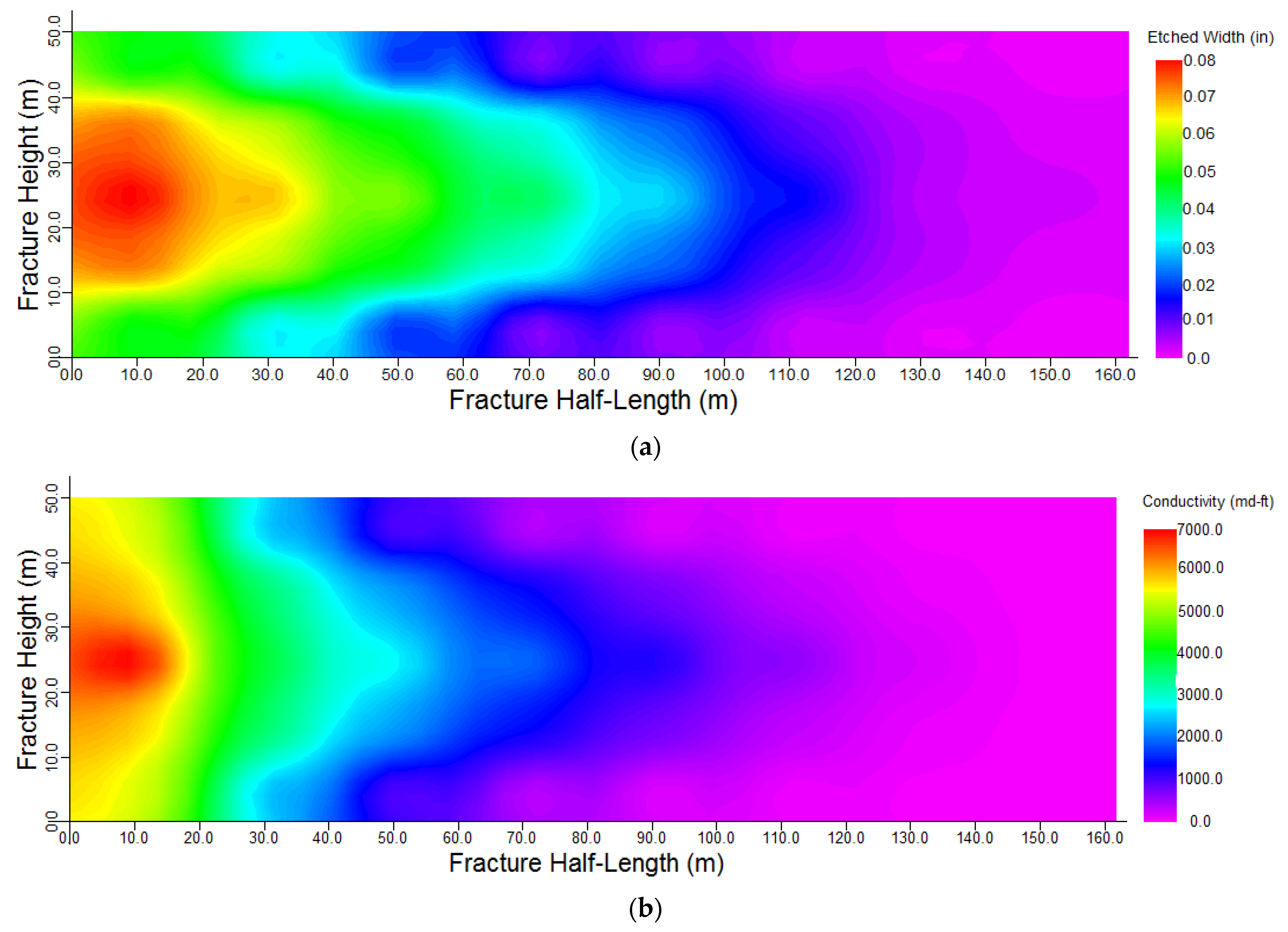
Acid concentration profiles are presented in Figure 4. Due to the decrease in fluid velocity along the fracture length, the acid concentration decreased in this direction. Additionally, acid leak-off into the fracture walls reduces the acid concentration along the fracture width. As shown in Figure 5, fracture width and conductivity profiles have maximum values in the center and decrease along the fracture length.

3.3. Optimization of Injection Parameters

In this section, injection parameters are optimized based on the proposed method and the input data listed in Table 1. The acid is assumed to be gelled hydrochloric (HCl) acid. In this study, the initial guess of flow rate ($q_{in}$ in the Figure 1) was 1 bbl/min. An initial acid concentration of 4.4 moles/dm³ (16% acid HCl) was selected. It should be mentioned that in all graphs of this section, the red point on each shape indicates the convergence condition.

3.3.1. Effect of Flow Rate on Optimization Results

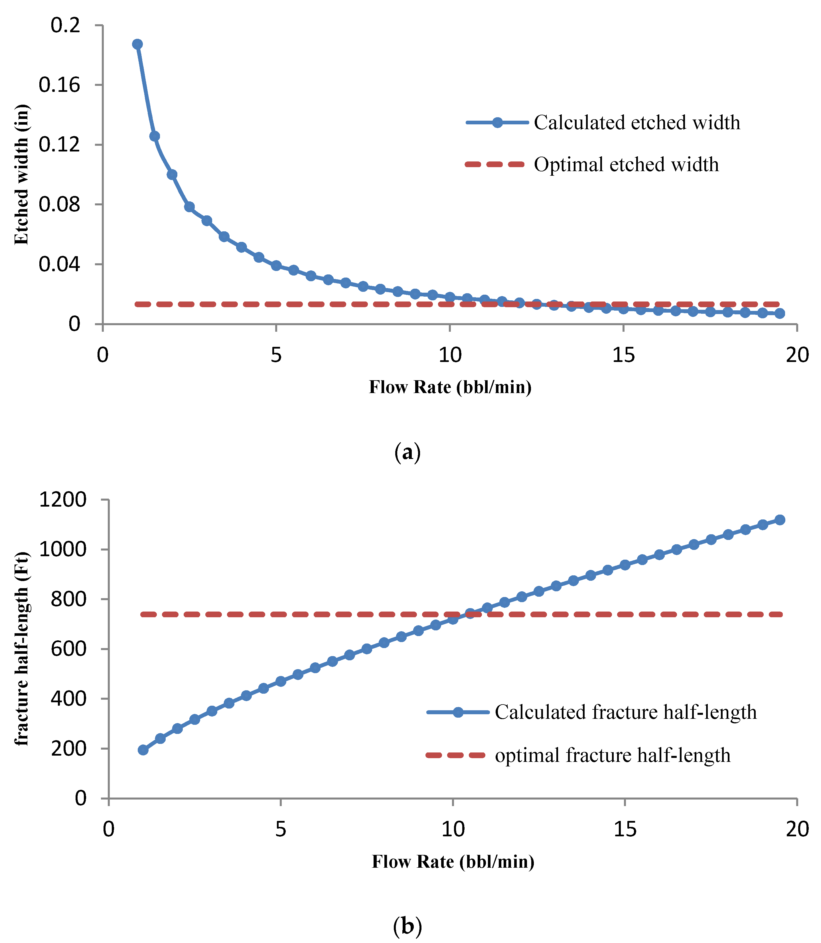
Figure 6 shows the flow rate changes versus the average acid-etched width and fracture half-length, respectively. When fluid velocity is low, the acid is more likely to diffuse the fracture surfaces, so the width created by the acid will be more significant. Furthermore, acid cannot penetrate through the fracture length resulting in a short maximum effective penetration distance. As the flow rate increases, acid more tends to penetrate along the fracture length. In other words, the convection phenomenon overcomes the acid diffusion into the fracture surfaces. Therefore, the maximum effective acid penetration distance increases and the average fracture width will be small. Therefore, with increasing flow rate, the fracture half-length increases, while average fracture width decreases. This process continues until each parameter reaches the value optimized by the UFD method. The calculated optimal fracture half-length and average fracture width are 738.16 Ft and 0.0133 in, respectively. Figure 7 shows the variation of the computational error with the flow rate. As the flow rate increases, the computational error decreases and reaches its minimum value in the flow rate of 12 bbl/min (the red point in Figure 7). After that, the computational error value increases because the optimal fracture half-length and average fracture width have deviated from their optimal values.

3.3.2. Effect of Acid Volume on Optimization Results

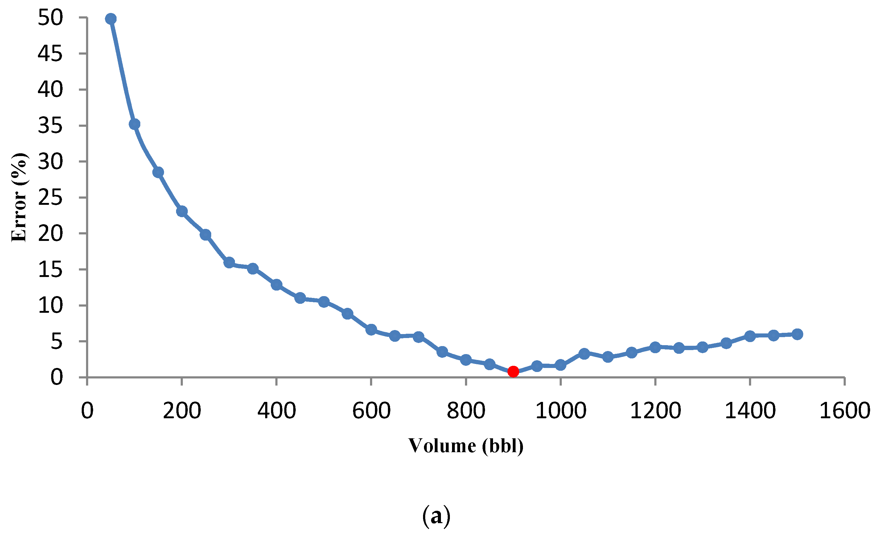
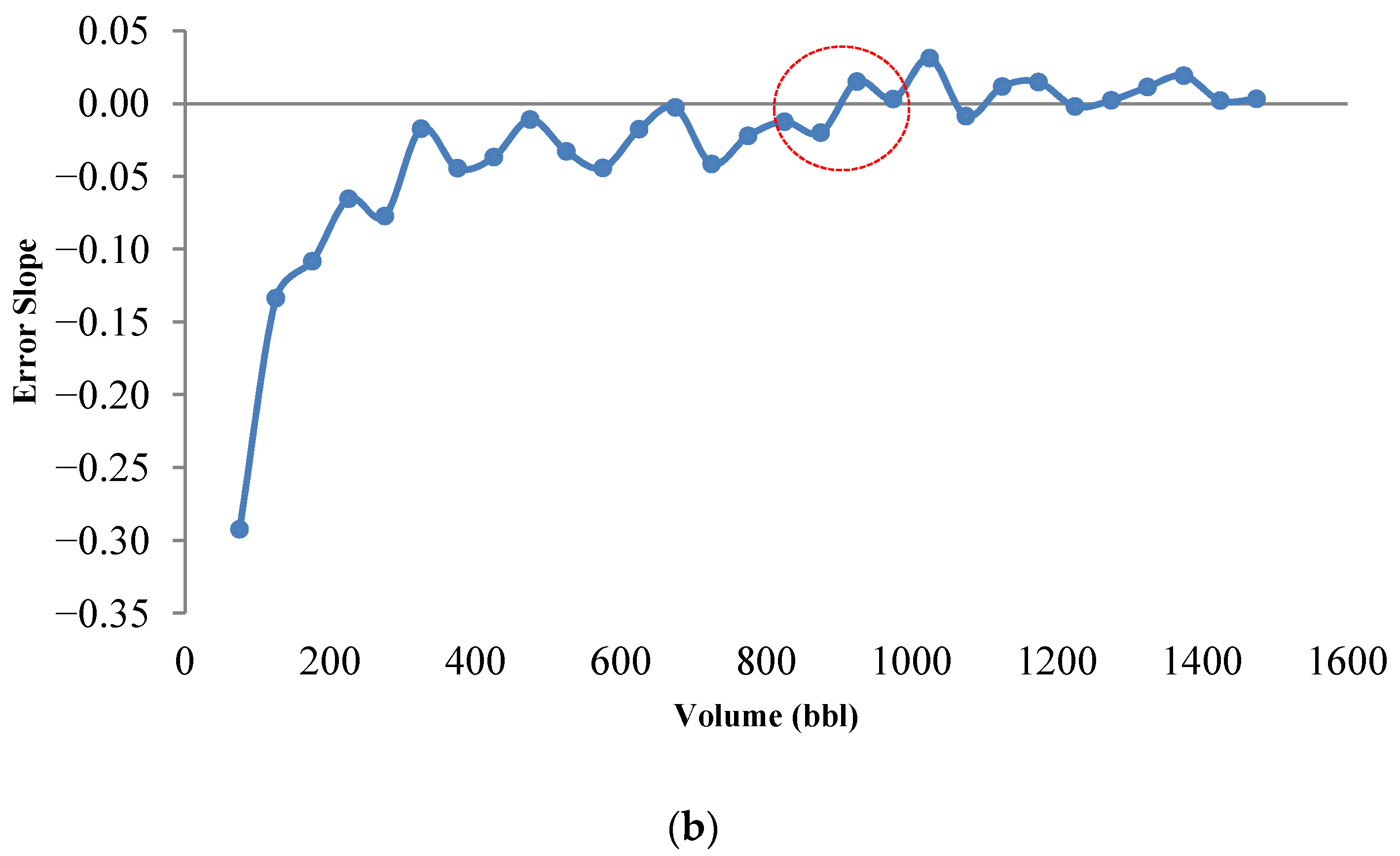
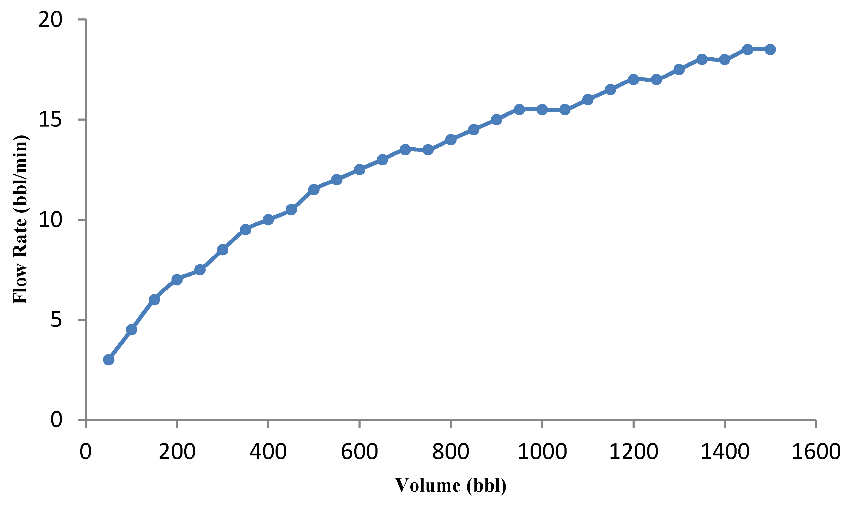
Acid volume significantly influences the acid fracturing treatment results. Since the acid volume change causes the optimal fracture geometry parameters and the optimal flow rate to change; in this study, the volume was changed for a specific range, and the minimum and maximum acid volumes, and the volume difference were selected as 50, 1500, and 50 bbl, respectively. The calculations continue until the last volume, and the minimum error is recorded in a specific volume for the following calculations. The minimum error changes versus acid volume graph are presented in Figure 8a. The calculated error value decreases as the volume increases and after reaching the minimum error value, the graph slope increases. The error-derived curve versus volume was also used to analyze the accuracy of results. According to Figure 8b, the error derivative starts with a steep slope and then slowly increases. The error derivative within the red circle in Figure 8b strikes the zero line for the first time. This collision is equivalent to the minimum error (red dot in Figure 8a). The volume calculated at this point is 900 bbl. Selecting a larger volume not only increases the treatment risk, operating costs will also rise significantly. The optimal flow rate for each acid volume was calculated, and the results are shown in Figure 9. If a high acid volume is selected, optimal fracture half-length and average fracture width estimated by the UFD method increase. These conditions can only be achieved at a high flow rate. In general, it has been proven that the optimal flow rate increases with the increase in acid volume [22]. For instance, the flow rate for 900 selected bbl is 15 bbl/min.

3.4. Parametric Study

In this section, the effect of the formation’s inherent properties (permeability and elastic properties) and controllable parameters (flow rheology, type, and acid percentage) on the optimal rate and volume are investigated. The input data are entered into the model according to Table 1, unless a specific parameter of this table is the purpose of evaluation. In all graphs of this section, the red dot represents optimum conditions.

3.4.1. Effect of Formation Permeability

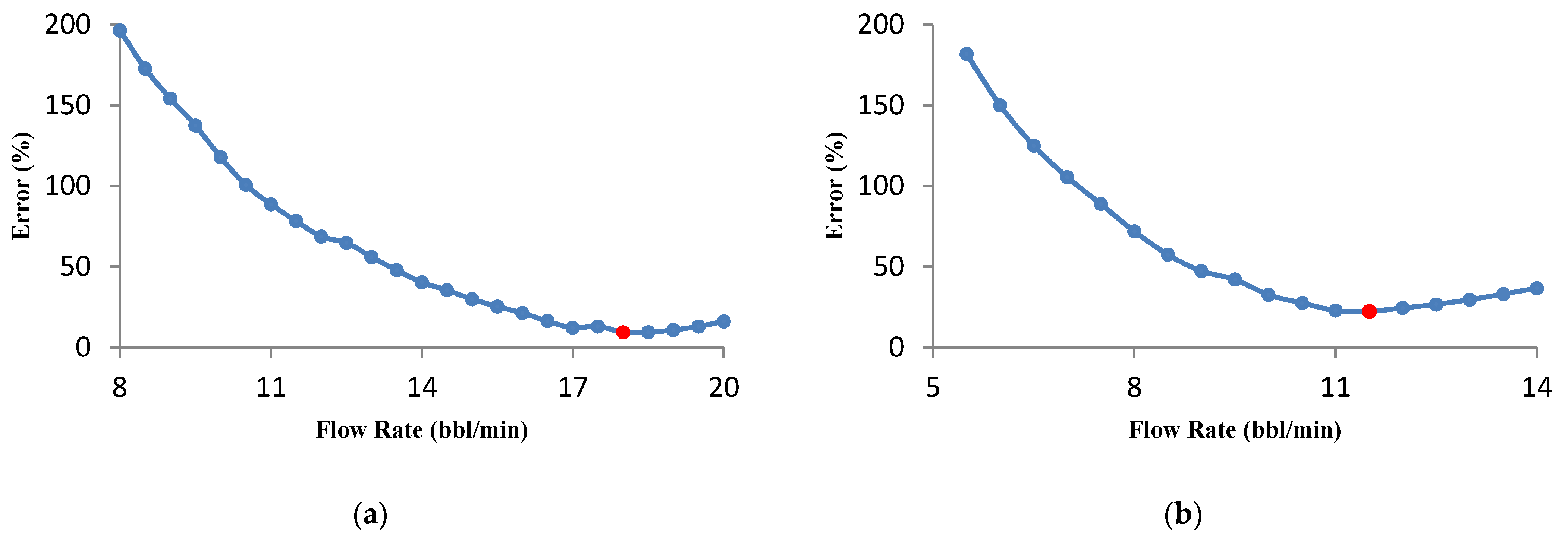
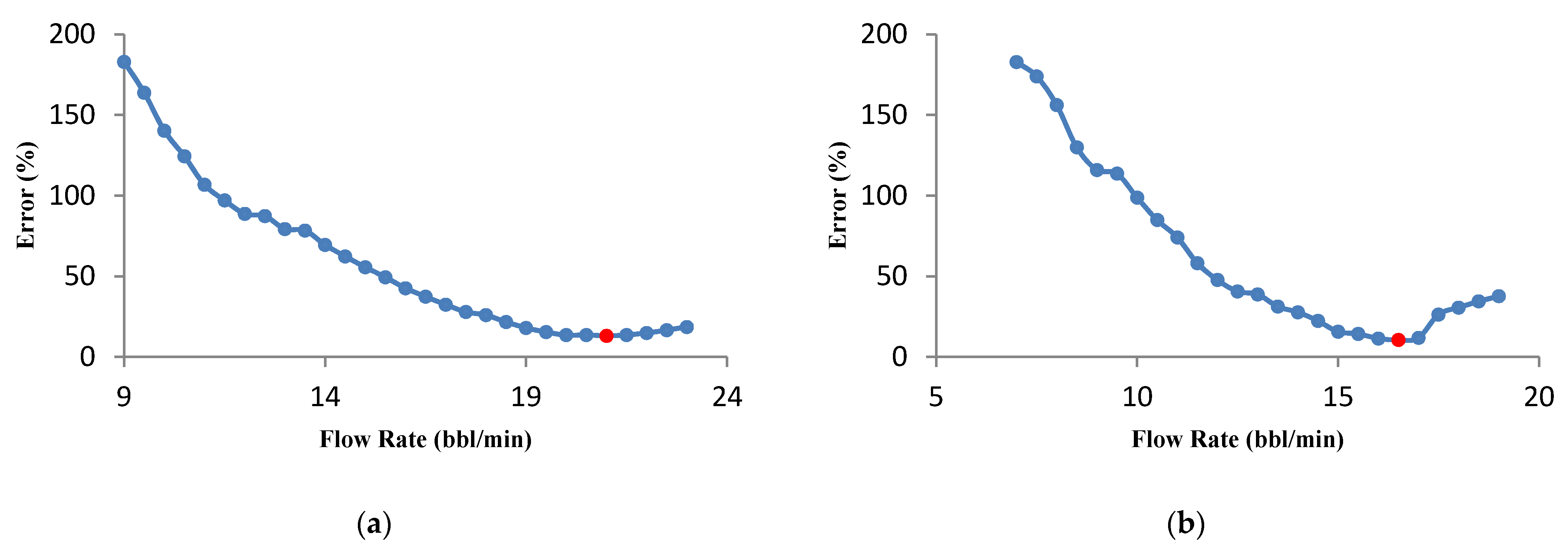
The formation permeability has a significant influence on the optimal fracture geometry parameters calculated by the UFD method. The effect of permeability for two samples with values of 0.1 and 0.001 md on the injection flow rate was investigated. The acid volume considered is 500 bbl. The flow rate–error graph for two samples is presented in Figure 10. It is desirable for low formation permeability to achieve a fracture with a high fracture half-length and small average fracture width. A higher flow rate will be required for the acid to penetrate deep into the fracture. The optimal flow rates for permeabilities of 0.001 and 0.1 md were calculated to be 18 and 11.5 bbl/min, respectively. To investigate the influence of the volume on the optimization results, the acid volume was increased to 1000 bbl, the calculations were repeated and the results are shown in Figure 11. If the volume of injected acid increases, the flow rate should be increased to approach the fracture geometry optimal condition. Therefore, the optimal flow rate increases for both samples. However, when permeability is 0.001 md, a higher flow rate is needed. The optimal flow rates for the permeability of 0.001 and 0.1 md were 21 and 16.5 bbl/min, respectively.

3.4.2. Effect of Injection Fluid Rheology

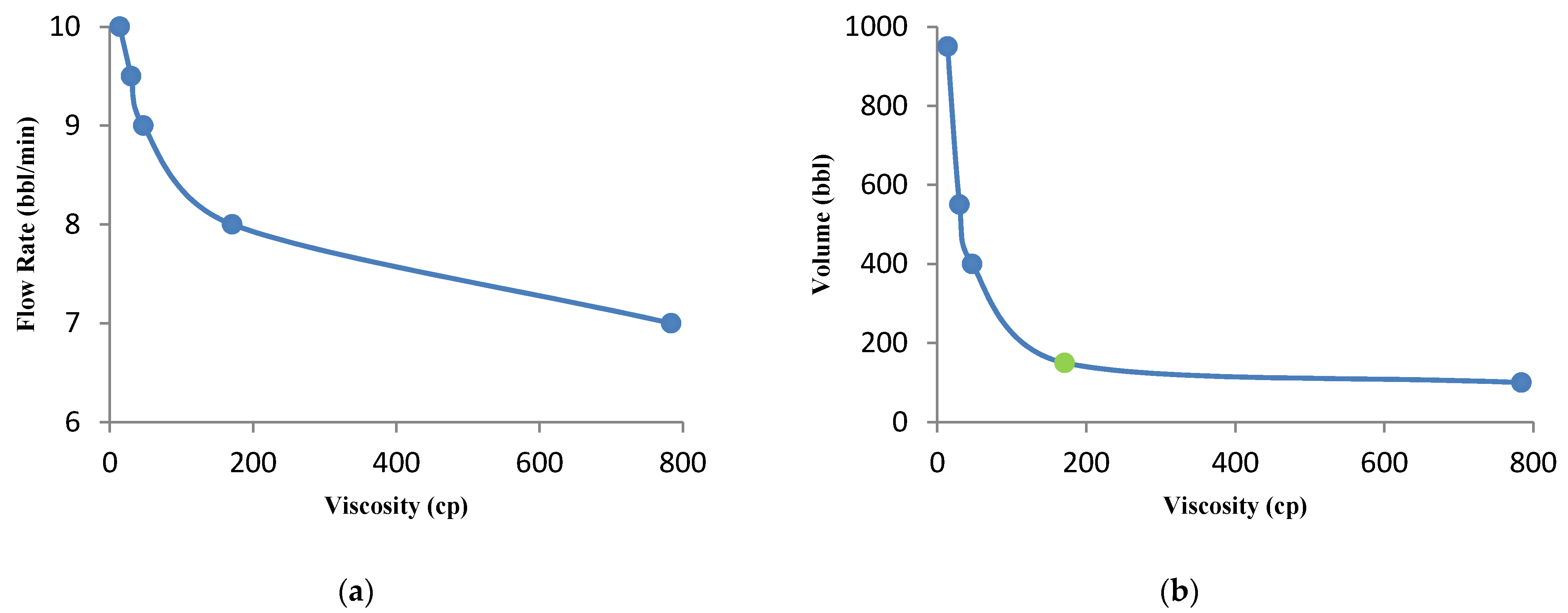
The viscosity of the injected fluid is one of the controllable parameters in hydraulic fracturing. Proper selection of this parameter can reduce costs and improve the results of hydraulic fracturing. The impact of different viscosities on injection flow rate is illustrated in Figure 12a. It should be noted that the viscosity refers to the fracture fluid viscosity as presented in

Table 3. Property of three acid systems types studied [37].

Acid Types	${\mathit{\mu }}_{\mathit{a}}\mathbf{\times }{\mathbf{10}}^{\mathbf{-}\mathbf{3}}\left(\mathbf{k}\mathbf{g}\mathbf{/}\mathbf{m}\mathbf{.}\mathbf{s}\right)$	${\mathit{D}}_{\mathit{e}\mathit{f}\mathit{f}}\mathbf{\left(}\mathbf{c}{\mathbf{m}}^{\mathbf{2}}\mathbf{/}\mathbf{s}\mathbf{\right)}$	n	$\mathit{K} \left(\mathbf{P}\mathbf{a}\mathbf{.}{\mathbf{s}}^{\mathbf{n}}\right)$
Straight	1	0.0000213	1.0	0.00109
Gelled	15	0.000008	0.65	0.05
Emulsified	30	2.64 × 10−8	0.675	0.315

[37]. For a low viscosity fluid (14 cp), higher flow rates (about 14 bbl/min) will be required to achieve optimization purposes. In contrast, for high viscosity fluid, a lower flow rate is needed. Fluid leak-off can be controlled in high viscosity values. Therefore, in such conditions, the required fluid flow rate is reduced.

It can be seen that more acid volume is required for low-viscosity fluid to achieve optimal fracture geometry parameters. As shown in Figure 12b, the curve slope is significantly steep for low viscosities (before the green dot). A slight increase in the fluid viscosity dramatically reduces the amount of acid required. After this point, the cure slope decreases, which means high viscosity has a negligible effect on reducing the acid volume. In general, increasing the fluid viscosity reduces the volume of acid required and thus reduces the cost of operation. However, increasing the fluid viscosity (after the green dot) does not significantly reduce the acid volume. On the other hand, supplying high viscosity fluid has many costs. Therefore, the optimal viscosity and volume of acid are 170 cp and 150 bbl, respectively.

3.4.3. Effect of the Acid Type

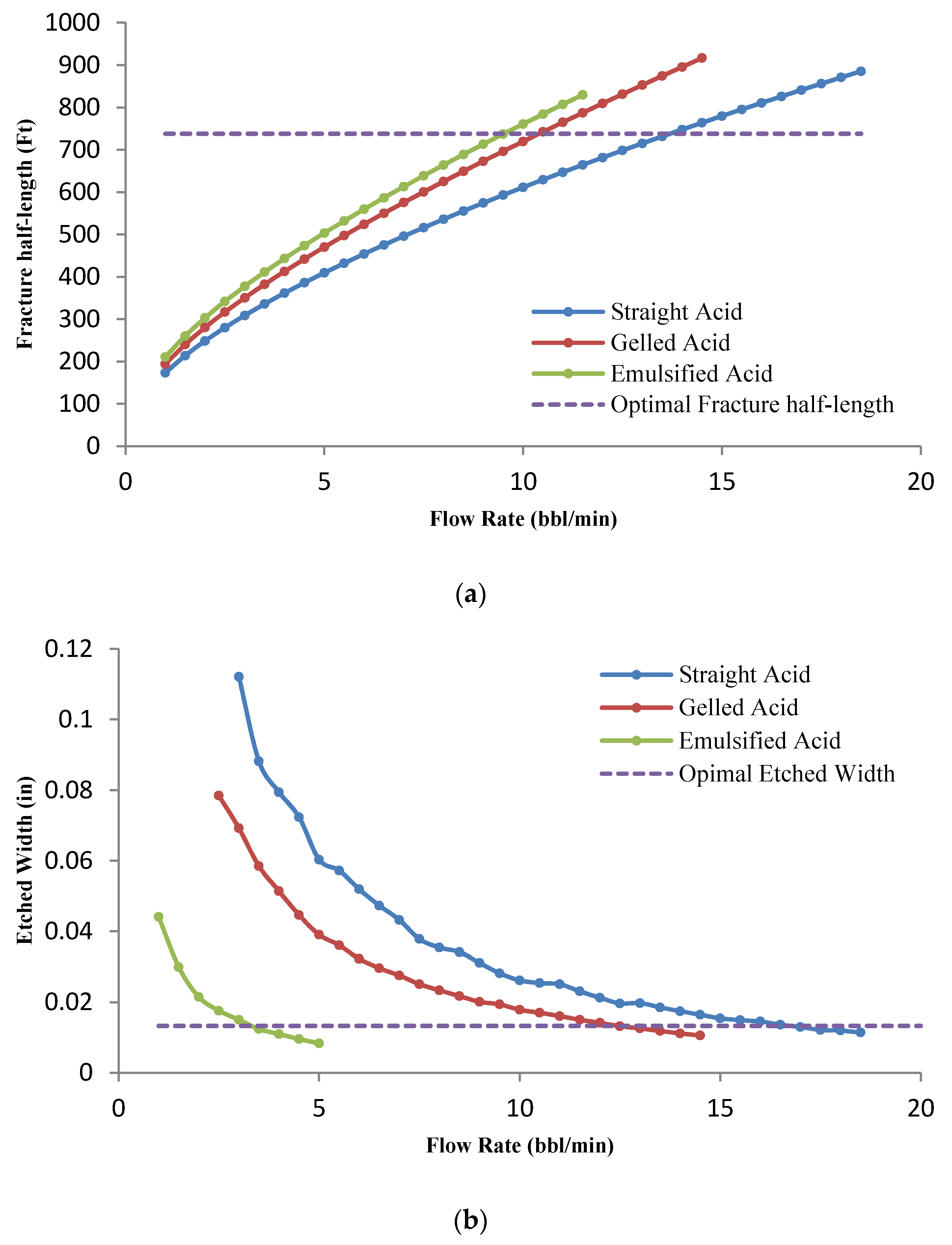
Different types of acid systems in the fracture will behave differently and affect acid optimization results. Straight acid is the simplest type of acid to which no viscosity enhancer or gel has been added. In acid fracturing, more complex acid systems are commonly used to reduce leak-off. In this section, three acid systems were studied, which are listed in Table 3 [37]. In order to investigate the effect of acid type on the flow rate, the acid volume was considered to be constant at 540 bbl. The other parameters are shown in Table 1. The flow rate optimization for the three types of acids is presented in Figure 13. The optimal flow rate for straight acid was calculated to be about 16.5 bbl/min.

However, optimal flow rates for gelled and emulsified acids are 12 and 11 bbl/min, respectively. In general, retarded acids have less uncertainty at a lower flow rate. The effect of the flow rate for three acid systems on the fracture half-length and average fracture width is shown in Figure 14. Due to its high diffusion coefficient, the straight acid can be less transported along the fracture length than the other two types of acids. Therefore, a higher flow rate is required to achieve the optimal fracture half-length (horizontal line in Figure 14a). On the other hand, straight acid will always create a higher average fracture width for a specified flow rate than the other two types. Therefore, only a high flow rate can bring the average fracture width closer to its optimal value (horizontal line in Figure 14b). However, for retarded acids, lower flow rates are required to achieve optimal fracture geometry goals.

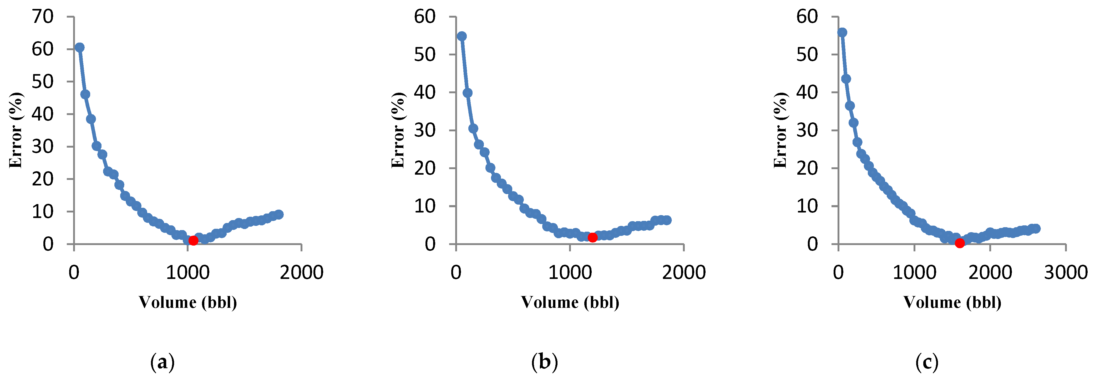
Figure 15 illustrates the effect of three types of acid system on acid volume. First, the error value decreases with increasing acid volume for all three types of acids, and after reaching its minimum value, the calculated error has gradually increased. The calculated optimal volumes for straight acid, gelled, and emulsified are 1050, 1200, and 1600 bbl, respectively. For the straight acid, fracture half-length and average fracture width are achieved to the optimum condition of fracture geometry in a smaller volume than the other two acid types by the UFD method. For retarded acids, the optimal conditions are obtained only in a high acid volume, as reported by [22].

3.4.4. Effect of the Acid Percentage

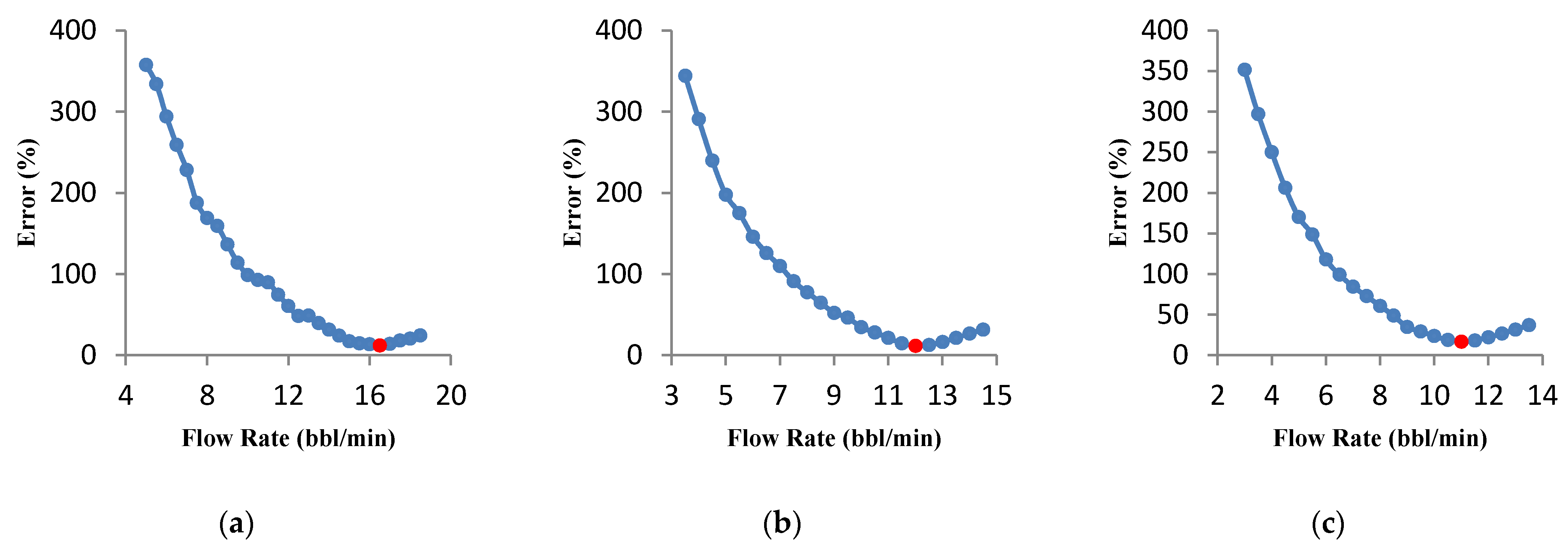
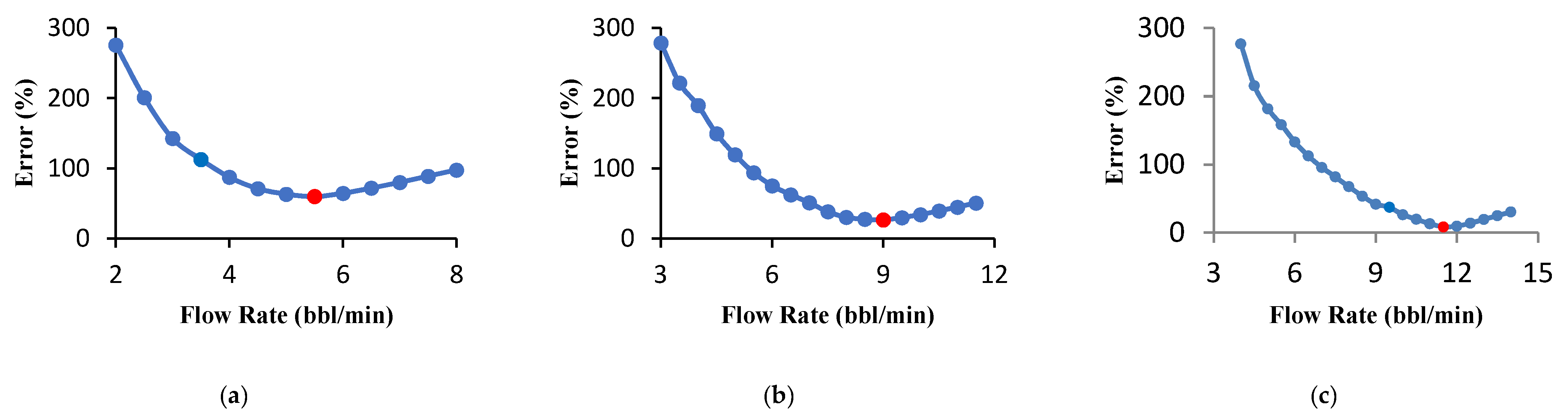
In order to investigate the effect of acid percentage on volume and flow rate, HCl gelled acids at 5, 10, and 15 percent were used. Figure 16 shows the effect of changes in acid percentage on the optimal flow rate. The optimal flow rate for 5%, 10%, and 15% acid concentrations were calculated to be 5.5, 9, and 11.5 bbl/min, respectively. As the acid percentage increases, the optimal flow rate increases. For higher acid percentages, the average fracture width increases. In this case, achieving the fracture geometry optimum condition by the UFD method will be possible only at a high flow rate. It should be noted that the difference between the estimated optimal flow rate in Figure 7 and Figure 13b (12 bbl/min) with Figure 16c (11.5 bbl/min) is due to acid concentration decreasing from 16% to 15%.

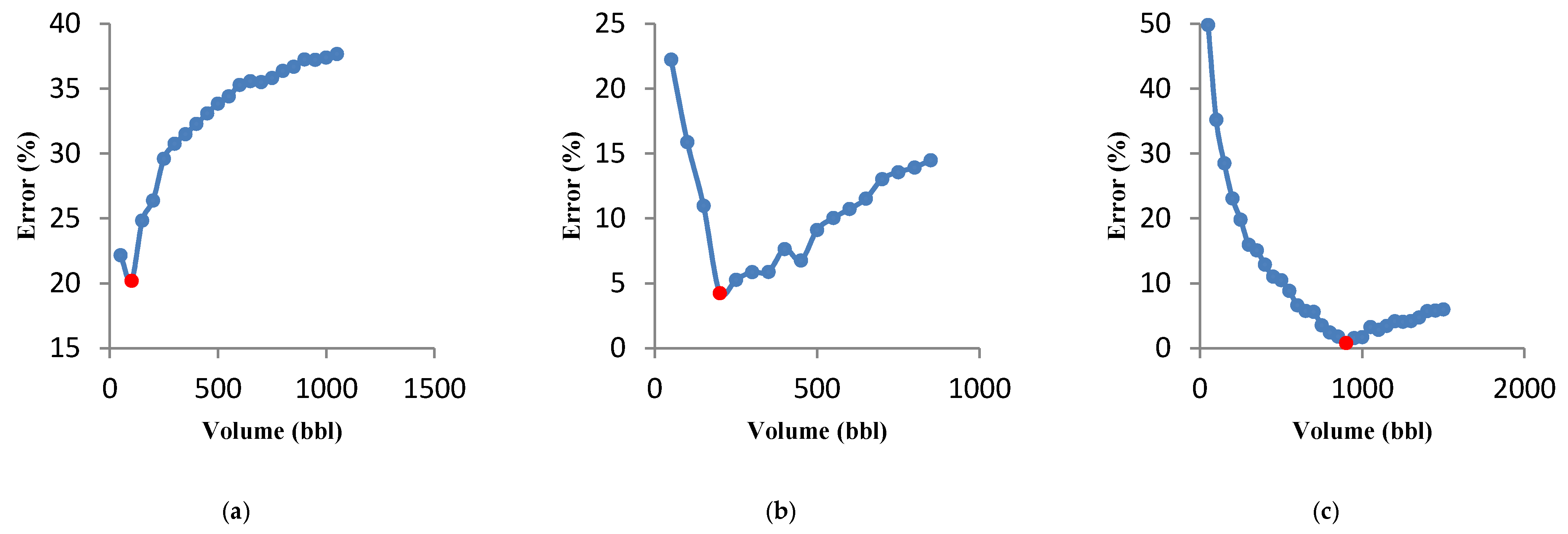
Additionally, the effect of acid concentration on the acid volume was investigated, and the results are presented in Figure 17. For an acid concentration of 5%, the optimal conditions appear at a low volume (about 100 bbl). If the acid concentration increases, optimal conditions can only be reached by increasing the acid volume. On the other hand, the acid volume should be increased to achieve the optimal parameters of the fracture geometry with a higher probability (less error). For instance, the optimal volumes for 10% and 15% acid concentrations were calculated to be 200 and 900 bbl, respectively.

3.4.5. Effect of the Young’s Modulus

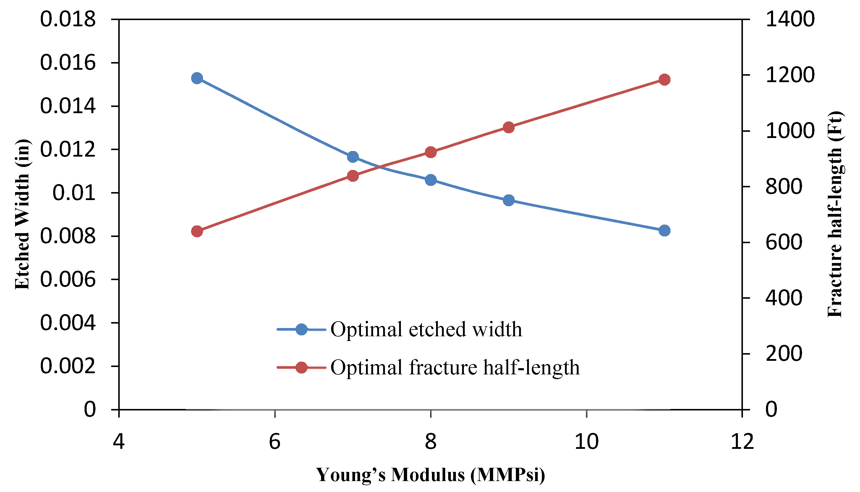
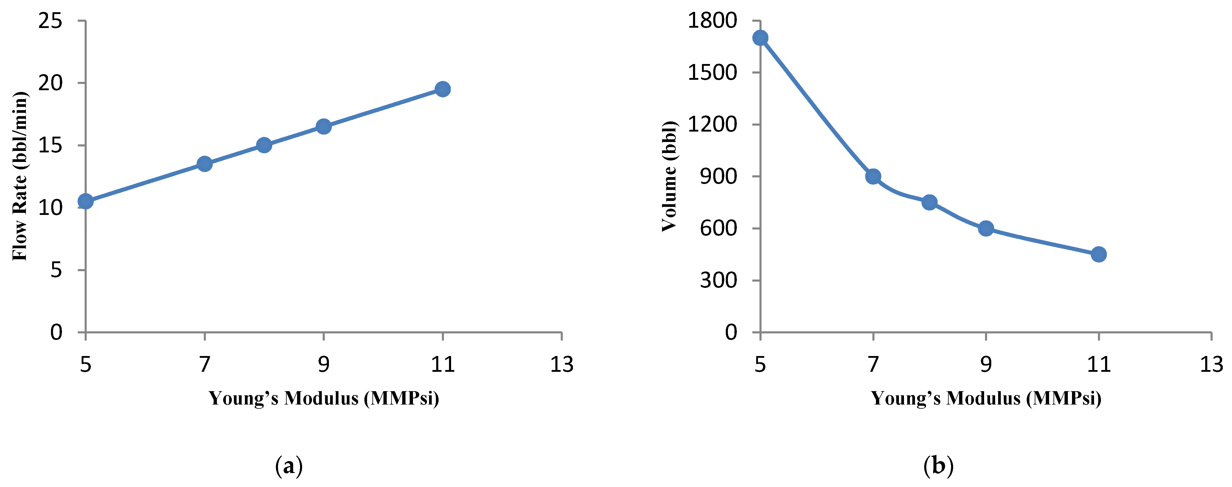
Mechanical properties of the formation have a significant influence on acid fracturing. Particularly, optimal injection parameters are affected by Young’s modulus and the formation closure stress. In this section, a gelled acid was selected with a volume of 540 bbl. The other parameters were kept constant, as listed in Table 1. The effect of the Young’s modulus on the fracture geometry optimal condition is shown in Figure 18. In addition, the flow rate optimization for different Young’s modulus was investigated, and the results are presented in Figure 19a. For a low Young’s modulus, a fracture with a small length and high average width is desirable, and the optimal fracture geometry parameters can be achieved at a low flow rate. However, as Young’s modulus increases, the optimal fracture geometry conditions reach a high flow rate. Besides, it was observed that the optimal acid volume decreases by increasing Young’s modulus (Figure 19b). So optimal fracture geometry parameters are determined to be high acid volume for a low Young’s modulus.

3.4.6. Effect of the Formation Closure Stress

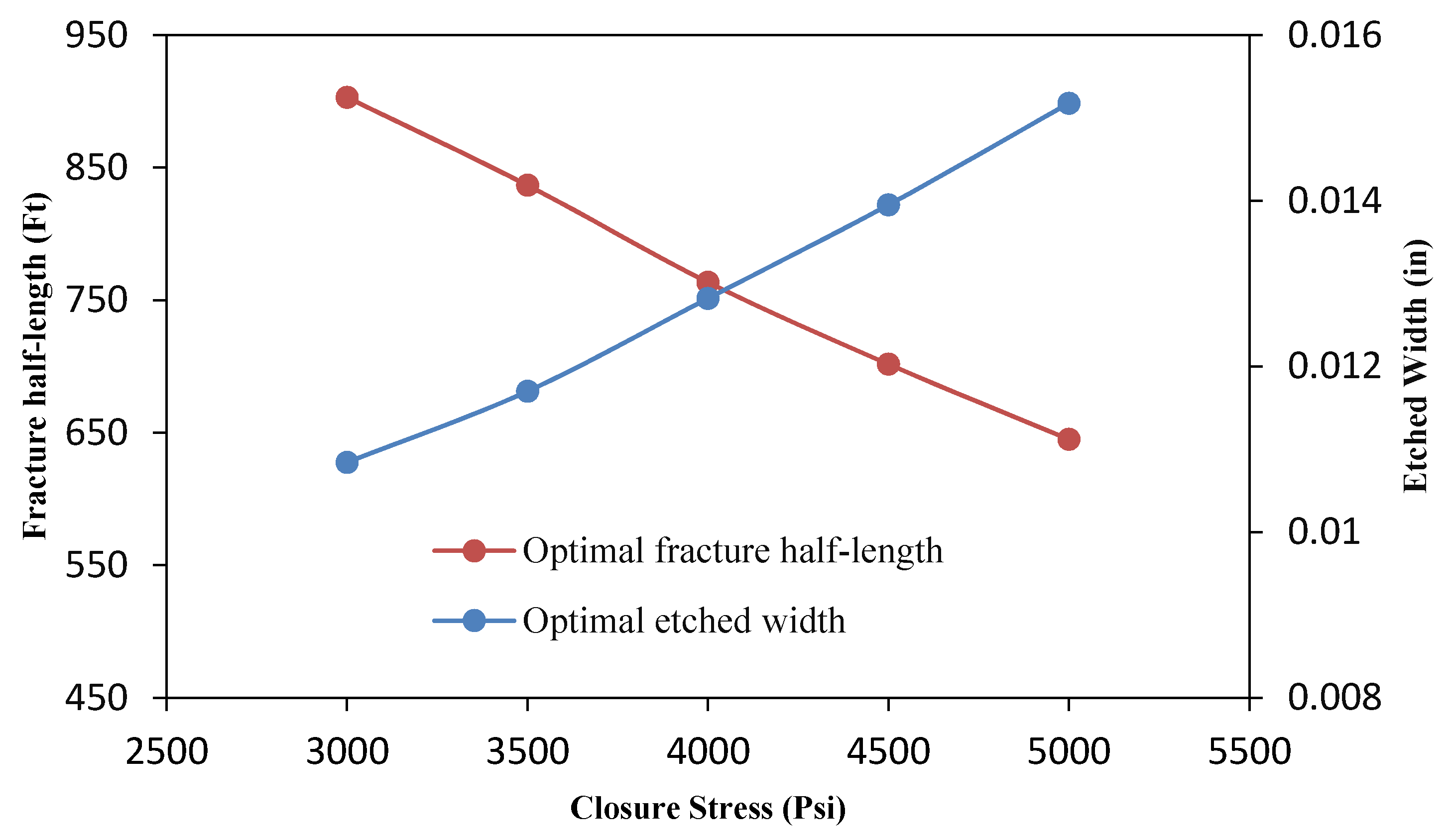
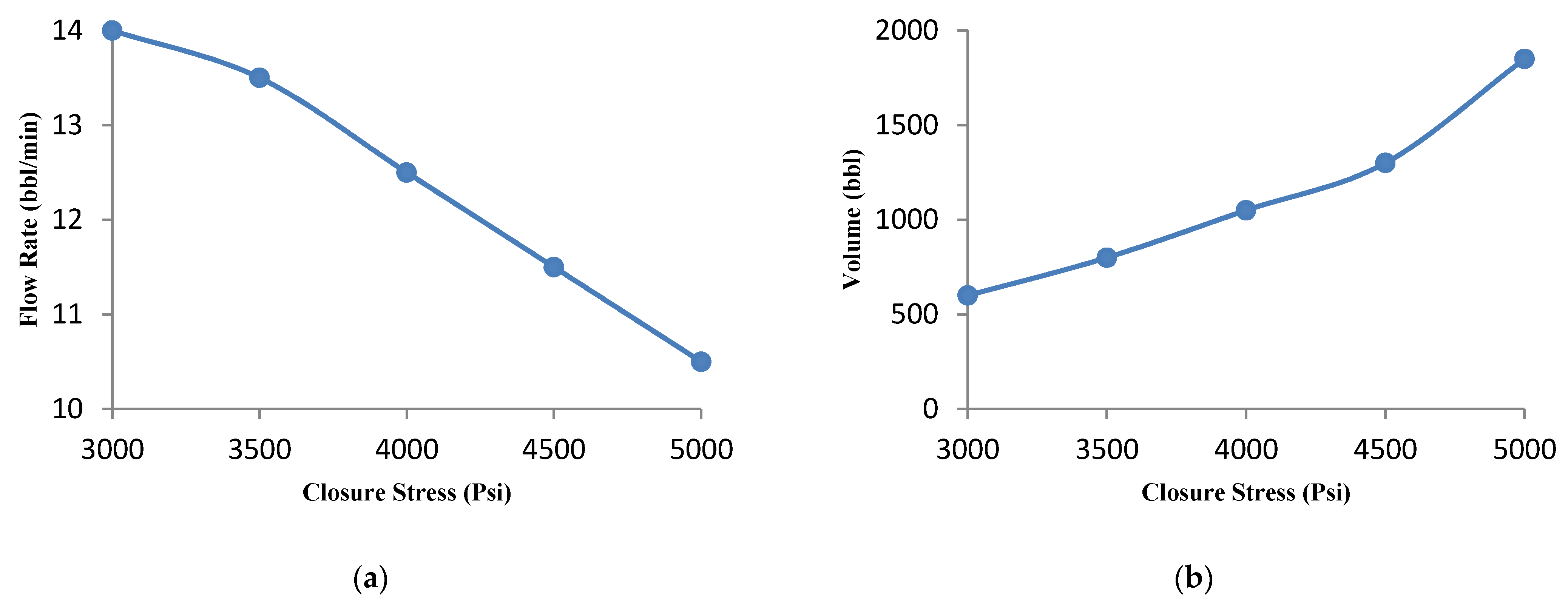
According to previous studies, the amount of formation closure stress directly affects fracture conductivity [28]. In addition, it indirectly affects the results of optimization of fracture geometry by the UFD method. Acid fracturing was suggested for formations with minimum horizontal stress (formation closure stress) less than 5000 Psi because the fracture face etching caused by the acid cannot support such high pressure [38]. Hence a 5000 Psi cut-off was considered for the formation closure stress. As the formation closure stress is increased, the calculated fracture half-length decreases and average fracture width by the UFD method increases (Figure 20). Therefore, optimal fracture geometry conditions reach a low flow rate. The effect of closure stress on the optimal flow rate was investigated, and the results are presented in Figure 21a. The effect of formation closure stress on acid volume is shown in Figure 21b. As the optimal closure stress increases, the acid volume increases. If the closure stress is high, the volume of injected acid should be increased to achieve the optimal fracture geometry parameters with high probability.

4. Conclusions

This research presents a method for optimal acid fracturing treatments by calculating optimal fracture geometry parameters. A new algorithm is performed to achieve the optimal fracture geometry parameters with the slightest uncertainty (maximum production index). The UFD method is implemented to optimize the fracture geometry parameters. The fracture propagation model is calculated by a pseudo-3D analytical method. In addition, a numerical method was implemented to simulate the acid transport model. The findings of case studies and sensitivity analyses can be considered as instructions for optimal acid fracturing design. Based on this study, the following conclusions can be summarized.

• Due to the large number of calculations, the simulations were performed with the proposed method for a specific case. The results have shown that the concentration of acid decreases along the fracture length and fracture walls. Acid-etched width and consequently, conductivity, decrease along the fracture length.
• The flow rate optimization for 16% gelled acid shows that the optimization results are influenced by the acid transport behavior within the fracture.
• The behavior of acid volume against minimum error (for a given volume) was investigated, and it was observed that the optimal flow rate increases with increasing acid volume.
• The parametric study shows that when formation permeability is decreased, the optimal fracture half-length and average fracture width increase and decrease, respectively. In this case, the optimal flow rate increases.
• Fluid viscosity is a controllable parameter during acid fracturing operations. As the fluid viscosity increases, the optimal flow rate and volume of the injected acid decrease. Therefore, increasing the fluid viscosity, to a certain extent, can improve the results of the acid fracturing treatment optimization. On the other hand, its excessive increase has no economic justification.
• Sensitivity analyses on three types of acid systems show that the optimal flow rate for straight acid is higher than for the other two types of acid. It was also observed that for retarded acids, the optimal conditions are reached only at a high acid volume.
• The acid percentage is an influential parameter on the results. For a 15% acid concentration, the required flow rate is higher than 5% and 10%. The acid volume must be increased to achieve optimal conditions for a sample with a high acid concentration.
• The parametric study shows that the optimal flow rate and acid volume increase and decrease, respectively, for high Young’s modulus. In addition, the effect of closure stress was also investigated and it was observed that for a sample with high closure stress, low flow rate and high acid volume are required.

References

- Roberts, L.D. The Effect of Surface Kinetics in Fracture Acidizing. Soc. Pet. Eng. J. 1974, 14, 385–395. [Google Scholar] [CrossRef]
- Williams, B.B.; Nierode, D.E. Design of Acid Fracturing Treatments. J. Pet. Technol. 1972, 24, 849–859. [Google Scholar] [CrossRef]
- Coulter, A.W.; Alderman, E.N.; Cloud, J.E.; Crowe, C.W. Mathematical Model Simulates Actual Well Conditions In Fracture Acidizing Treatment Design. In Proceedings of the Fall Meeting of the Society of Petroleum Engineers of AIME, Houston, TX, USA, 6–9 October 1974. [Google Scholar] [CrossRef]
- Schechter, R.S. Oil Well Stimulation; Prentice-Hall, Inc.: Englewood Cliffs, NJ, USA, 1992. [Google Scholar]
- Berman, A.S. Laminar Flow in Channels with Porous Walls. J. Appl. Phys. 1953, 24, 1232–1235. [Google Scholar] [CrossRef]
- Hill, A.D.; Zhu, D.; Wang, Y. The Effect of Wormholing on the Fluid Loss Coefficient in Acid Fracturing. SPE Prod. Facil. 1995, 10, 257–264. [Google Scholar] [CrossRef]
- Gdanski, A.D.; Lee, W.S. On the Design of Fracture Acidizing Treatments. In Proceedings of the SPE Production Operations Symposium, Oklahoma City, OK, USA, 13–14 March 1989. [Google Scholar] [CrossRef]
- Navarrete, R.; Miller, M.; Gordon, J. Laboratory and Theoretical Studies for Acid Fracture Stimulation Optimization. In Proceedings of the 1998 SPE Permian Basin Oil and Gas Recovery Conference, Midland, TX, USA, 23–26 March 1998. [Google Scholar] [CrossRef]
- Lo, K.K.; Dean, R.H. Modeling of Acid Fracturing. SPE Prod. Eng. 1989, 4, 194–200. [Google Scholar] [CrossRef]
- Settari, A.; Sullivan, R.; Hansen, C. A New Two-Dimensional Model for Acid-Fracturing Design. SPE Prod. Facil. 2001, 16, 200–209. [Google Scholar] [CrossRef]
- Romero, J.; Gu, H.; Gulrajani, S.N. 3D Transport in Acid-Fracturing Treatments: Theoretical Development and Consequences for Hydrocarbon Production. SPE Prod. Facil. 2001, 16, 122–130. [Google Scholar] [CrossRef]
- Mou, J.; Zhu, D.; Hill, A.D. Acid-Etched Channels in Heterogeneous Carbonates—A Newly Discovered Mechanism for Creating Acid-Fracture Conductivity. SPE J. 2009, 15, 404–416. [Google Scholar] [CrossRef]
- Oeth, C.V.; Hill, A.D.; Zhu, D. Acid Fracture Treatment Design with Three-Dimensional Simulation. In Proceedings of the SPE Hydraulic Fracturing Technology Conference, The Woodlands, TX, USA, 4–6 February 2014. [Google Scholar] [CrossRef]
- Aljawad, M.S.; Zhu, D.; Hill, A.D. Modeling Study of Acid Fracture Fluid System Performance. In Proceedings of the SPE Hydraulic Fracturing Technology Conference, The Woodlands, TX, USA, 9–11 February 2016. [Google Scholar] [CrossRef]
- Alhubail, M.M.; Misra, A.; Barati, R. A Novel Acid Transport Model with Robust Finite Element Discretization. In Proceedings of the SPE Kingdom of Saudi Arabia Annual Technical Symposium and Exhibition, Dammam, Saudi Arabia, 24–27 April 2017. [Google Scholar] [CrossRef]
- Ugursal, A.; Schwalbert, M.P.; Zhu, D.; Hill, A.D. Acid Fracturing Productivity Model for Naturally Fractured Carbonate Reservoirs. In Proceedings of the SPE International Hydraulic Fracturing Technology Conference and Exhibition, Muscat, Oman, 16–18 October 2018. [Google Scholar] [CrossRef]
- Dang, L.; Zhou, C.; Huang, M.; Jiang, D. Simulation of effective fracture length of prepad acid fracturing considering multiple leak-off effect. Nat. Gas Ind. B 2019, 6, 64–70. [Google Scholar] [CrossRef]
- Ben-Naceur, K.; Economides, M.J. Design and Evaluation of Acid Fracturing Treatments. In Proceedings of the SPE Joint Rocky Mountain Regional/Low Permeability Reservoirs Symposium and Exhibition, Denver, Colorado, 6–8 March 1989. [Google Scholar] [CrossRef]
- Guo, J.; Li, Y.; Zhao, J.; Luo, J. Research of Three-Dimensional Model for Acid Fracturing and Optimum Design For the Treatments. In Proceedings of the Canadian International Petroleum Conference, Calgary, Alberta, 8–10 June 2004. [Google Scholar] [CrossRef]
- Ravikumar, A.; Marongiu-Porcu, M.; Morales, A. Optimization of Acid Fracturing with Unified Fracture Design. In Proceedings of the Abu Dhabi International Petroleum Exhibition and Conference, Abu Dhabi, United Arab Emirates, 9–12 November 2015. [Google Scholar] [CrossRef]
- Ai, K.; Duan, L.; Gao, H.; Jia, G. Hydraulic Fracturing Treatment Optimization for Low Permeability Reservoirs Based on Unified Fracture Design. Energies 2018, 11, 1720. [Google Scholar] [CrossRef] [Green Version]
- Aljawad, M.S.; Schwalbert, M.P.; Zhu, D.; Hill, A.D. Optimizing Acid Fracture Design in Calcite Formations: Guidelines Using a Fully Integrated Model. SPE Prod. Oper. 2020, 35, 161–177. [Google Scholar] [CrossRef]
- Aljawad, M.S.; Zhu, D.; Hill, A.D. Temperature and Geometry Effects on the Fracture Surfaces Dissolution Patterns in Acid Fracturing. In Proceedings of the SPE Europec featured at 80th EAGE Conference and Exhibition, Copenhagen, Denmark, 11–14 June 2018. [Google Scholar] [CrossRef]
- Aljawad, M.S. Impact of Diversion on Acid Fracturing of Laminated Carbonate Formations: A Modeling Perspective. ACS Omega 2020, 5, 6153–6162. [Google Scholar] [CrossRef] [PubMed]
- Al-Ameri, A.; Gamadi, T. Optimization of acid fracturing for a tight carbonate reservoir. Petroleum 2020, 6, 70–79. [Google Scholar] [CrossRef]
- Hassan, A.; Aljawad, M.S.; Mahmoud, M. An Artificial Intelligence-Based Model for Performance Prediction of Acid Fracturing in Naturally Fractured Reservoirs. ACS Omega 2021, 6, 13654–13670. [Google Scholar] [CrossRef] [PubMed]
- Valko, M.J.; Economides, P. Hydraulic Fracturing Mechanics; John Wiley and Sons: New York, NY, USA, 1995. [Google Scholar]
- Deng, J.; Mou, J.; Hill, A.D.; Zhu, D. A New Correlation of Acid-Fracture Conductivity Subject to Closure Stress. SPE Prod. Oper. 2012, 27, 158–169. [Google Scholar] [CrossRef]
- Oeth, C.V. Three-dimensional Modeling of Acid Transport and Etching in a Fracture. Ph.D. Thesis, Texas A & M University, College Station, TX, USA, 2013. Available online: https://hdl.handle.net/1969.1/151892 (accessed on 30 November 2021).
- Economides, M.J.; Oligney, R.E.; Valko, P.P. Unified Fracture Design; Orsa Press: Alvin, TX, USA, 2002. [Google Scholar]
- Crank, J. Free and Moving Boundary Problems; Clarendon Press: New York, NY, USA, 1984. [Google Scholar]
- Mou, J. Modeling Acid Transport and Non-Uniform Etching in a Stochastic Domain in Acid Fracturing. Ph.D. Thesis, Texas A&M University, College Station, TX, USA, 2009. [Google Scholar]
- Acharya, S.; Moukalled, F.H. Improvements to incompressible flow calculation on a nonstaggered curvilinear grid. Numer. Heat Transfer Part B Fundam. 1989, 15, 131–152. [Google Scholar] [CrossRef]
- Penny, G.S.; Conway, M.W. Fluid Leak-off. In Recent Advances in Hydraulic Fracturing; Gidley, J.L., Holditch, S.A., Nierode, D.E., Veatch, R.W., Jr., Eds.; Society of Petroleum: Richardson, TX, USA, 1989; pp. 147–176. [Google Scholar]
- Settari, A. Modeling of Acid-Fracturing Treatments. SPE Prod. Facil. 1993, 8, 30–38. [Google Scholar] [CrossRef]
- Terrill, R.M. Heat transfer in laminar flow between parallel porous plates. Int. J. Heat Mass Transf. 1965, 8, 1491–1497. [Google Scholar] [CrossRef]
- De Rozieres, J. Measuring Diffusion Coefficients in Acid Fracturing Fluids and Their Application to Gelled and Emulsified Acids. In Proceedings of the SPE Annual Technical Conference and Exhibition, New Orleans, Louisiana, 25–28 September 1994. [Google Scholar] [CrossRef]
- Valko, P.; Norman, L.; Daneshy, A. Petroleum Well Construction (Book)|Etdeweb; Well Stimulation; Wiley: Hoboken, NJ, USA, 1998; Chapter 17; p. 506. Available online: https://www.osti.gov/Etdeweb/Biblio/300026 (accessed on 30 November 2021).
Figure 1.
Flowchart of the proposed method.
Figure 2.
The domain of the acid model.
Figure 3.
Comparison between the calculated acid concentration along the fracture at different Peclet numbers using the proposed model and the Terrill, 1965 method [36].
Figure 4.
Simulated acid concentration within the fracture domain for a flow rate of 10 bbl/min and 400 bbl acid volume. (a) fracture half-length vs. height (b) fracture half-length vs. width.
Figure 5.
Acid-etched width (a) and fracture conductivity (b) distribution in the fracture domain for a flow rate of 10 bbl/min and 400 bbl acid volume.
Figure 6.
The average acid-etched width (a) and fracture half-length (b) versus injection flow rate.
Figure 7.
Computational error by changing the injection flow rate for an acid volume of 540 bbl.
Figure 8.
Minimum computational error for a given volume (a). Error derivative changes versus acid volume (b).
Figure 9.
Optimal flow rate changes versus acid volume.
Figure 10.
The influence of formation permeability on the optimal injection flow rate for a 500 bbl Acid Volume. (a) K = 0.001 md and (b) K = 0.1 md.
Figure 11.
The influence of formation permeability on the optimal injection flow rate for a 1000 bbl acid volume. (a) K = 0.001 md and (b) K = 0.1 md.
Figure 12.
The impact of fluid viscosity on the of flow rate (a) and acid volume (b) for a 540 bbl acid volume.
Figure 13.
Results of flow rate optimization for three acid systems types investigated for a 540 bbl acid. (a) straight acid, (b) gelled acid, and (c) emulsified acid.
Figure 14.
Variations of fracture half-length (a) and average etched width (b) with flow rate for three acid system types.
Figure 15.
Results of acid volume optimization for three acid systems types. (a) straight acid, (b) gelled acid, and (c) emulsified acid.
Figure 16.
The effect of acid concentration on the flow rate optimization results for a 540 bbl acid volume. (a) 5 wt % acid, (b) 10 wt % acid, and (c) 15 wt % acid.
Figure 17.
The effect of acid concentration on acid volume optimization results. (a) 5 wt % acid, (b) 10 wt % acid, and (c) 15 wt % acid.
Figure 18.
Optimal fracture half-length and etched width vs. Young’s modulus.
Figure 19.
The impact of Young’s modulus on the flow rate (a) and acid volume (b) for a 540 bbl acid volume.
Figure 20.
Optimal fracture half-length and etched width vs. closure stress.
Figure 21.
The influence of formation closure stress on the flow rate (a) and acid volume (b) for a 540 bbl acid volume.