Generation of Realistic Boundary Conditions at the Combustion Chamber/Turbine Interface Using Large-Eddy Simulation

Abstract

Numerical simulation of multiple components in turbomachinery applications is very CPU-demanding but remains necessary in the majority of cases to capture the proper coupling and a reliable flow prediction. During a design phase, the cost of simulation is, however, an important criterion which often defines the numerical methods to be used. In this context, the use of realistic boundary conditions capable of accurately reproducing the coupling between components is of great interest. With this in mind, this paper presents a method able to generate more realistic boundary conditions for isolated turbine large-eddy simulation (LES) while exploiting an available integrated combustion chamber/turbine LES. The unsteady boundary conditions to be used at the inflow of the isolated turbine LES are built from the modal decomposition of the database recorded at the interface between the two components of the integrated LES simulation. Given the reference LES database, the reconstructed field boundary conditions can then be compared to standard boundary conditions in the case of isolated turbine configuration flow predictions to illustrate the impact. The results demonstrate the capacity of this type of conditions to reproduce the coupling between the combustion chamber and the turbine when standard conditions cannot. The aerothermal predictions of the blade are, in particular, very satisfactory, which constitutes an important criterion for the adoption of such a method during a design phase.

1. Introduction

The coupling effect on the flow of different components of a turbomachine is a subject of primary importance for engine manufacturers. The behavior and the performance of an isolated component is indeed often largely altered when installed in a complete configuration, degrading the performance and/or the lifespan of the engine in certain cases. Numerically, it is possible to study these phenomena by performing integrated simulations of several components of a turbomachine. These unsteady simulations, although very complex to implement, are often required to correctly capture the spatial and temporal interactions that appear at interfaces. This is usually carried out using large-eddy simulation (LES) to capture the unsteadiness of the phenomena. In addition, because of stability constraints, the number of blades in the different stages of a turbomachine most often do not share any common divider, which means that, numerically, the complete configuration cannot be divided into smaller sectors using periodicity conditions. Thus, to be able to accurately simulate the multicomponent coupling without reducing the number of blades or without additional simplifying assumptions, the best option is to perform a 360${}^{\circ }$ simulation of the complete turbomachine. Despite the constant progress in computing capabilities, very few examples of complete engine simulations are available in the literature (even fewer using LES) and in any case, these simulations remain very expensive [1,2,3,4]. As a result, and for engine manufacturers, this solution is not feasible today during the design phases, and other options must be considered. One of the keys to the robust and efficient use of simulation in industry therefore rests on the ability to reproduce, as accurately as possible, the effect of an upstream component on the isolated simulation of the component of interest. This observation accentuates the importance of boundary conditions (upstream and downstream boundary conditions) of any given simulation of given components.

This topic is particularly relevant in the study of the coupling between a combustion chamber and a turbine. In that case, numerical simulation is a great tool to develop and design new geometries while still meeting the demanding constraints of wall temperature requirements, operating points, and off-design capabilities. In such applications, where the goal is to simulate an isolated turbine, the main challenge lies in the accurate prediction of the inlet flow by taking into account the high levels of turbulence, the residual swirl, and the temperature nonuniformities generated by the chamber. A previous study carried out by Duchaine et al. [5] has shown that standard synthetic turbulence injection methods are not sufficient to recover the complex behavior of such flow.

The objective here is to understand the use of realistic boundary conditions applied to an isolated turbine by taking into account the flow unsteadiness at the interface between the components (the present methodology can however be applied to other components). The ability to reproduce the complex dynamics of turbulent flows by a small number of the most energetic modes is, therefore, crucial to analyze and model complex physics at a relatively low memory cost. Proper orthogonal decomposition (POD) is commonly used to extract spatial orthogonal modes from a series of snapshots of the flow at different physical times. In its standard form, the POD [6,7] is computed in the time domain, but it can also be reformulated in the frequency domain. In this case, the method is called spectral proper orthogonal decomposition [8]. As a consequence of this shift, the modes obtained vary both spatially and temporally and are orthogonal with a spatiotemporal dot product. Note also that the choice of the dot product is crucial for boundary condition reconstruction, as many variables are needed for the flow solver. In the following, this dot product will be chosen to correctly study the spatiotemporal consistency of the database as detailed below. By extracting the most energetic frequencies at the inlet, it is then possible to create unsteady inlet boundary conditions with realistic velocity and temperature fluctuations. The objective is to understand which phenomenon occurring in the flow exiting combustion chamber is of importance for the simulation of the turbine stage. Knowing these aspects will help to design adapted inlet conditions based on numerical database of a combustor for different operating conditions of a turbine stage. Such a study also allows us to better understand the sensitivity of turbine flows to inlet conditions for fundamental analysis but also for design purposes of both combustors and turbine blades. A similar reconstruction method has, for example, been used by Ghate [9] to reproduce the wake of a cylinder placed in a flow.

Despite the ability to analyze the spatiotemporal coherence of an initial database, the use of SPOD raises questions that must be considered. First, the choice of the scalar product will impact the spectrum obtained by the SPOD method. In a configuration whose aim is to study the combined effect of the migration of a hot spot and of a swirling flow on the aerothermal properties of the turbine, the scalar product chosen should take into account the velocity and the temperature at the interface. Second, to reduce the overall cost of storing the recorded database, partial reconstructions are created, which raises the question of the impact of the omitted information on the inlet boundary condition obtained. Finally, the use of SPOD is significantly more complex to set up compared to standard inlet boundary conditions usually used in industry and which exploit constant time-averaged values or 2D maps. The contributions of this method must therefore be substantial to justify its use and appear as a credible candidate in different configurations compared to standard boundary conditions.

This paper is organized into three main parts. The first part introduces the integrated FACTOR configuration, composed of the combustion chamber and the HP vanes, which will be used to apply the SPOD method. In particular, the plane at the interface between the chamber and the turbine is recorded at regular intervals to generate an unsteady database from the LES. Then, through two modal decompositions, the information related to the coupling between the two components is extracted and analyzed. Then, in a second part, the SPOD is used to generate realistic conditions for the isolated turbine configuration via partial reconstructions of the numerical database. To finish, the new type of unsteady boundary conditions are compared in a third part to more traditional boundary conditions, and the integrated chamber/turbine simulation is carried out to demonstrate its ability to accurately reproduce multicomponent coupling, although isolated turbine simulations are conducted.

2. Combustion Chamber/Turbine Integrated Simulation

The configuration that will be the subject of the study comes from the European FACTOR project. In summary, the FACTOR project was dedicated to the analysis of interactions between lean-burn combustion chambers and high-pressure turbines. This project generated experimental data around two test rigs: a tri-sector combustion chamber studied at UNIFI [10] and a complete annular chamber equipped with its HP turbine stage installed at DLR Goettingen [11]. The objective of the present study is to understand the interactions and the coupling between the combustion chamber and the turbine, by means of advanced diagnostics such as SPOD. To do so, the configuration studied is limited to the plenum, the combustion chamber, and the fixed stage of the turbine (Figure 1).

The interaction of the combustion chamber with a turbine located downstream is a very important subject for engine manufacturers. Thus, several studies have already been made on various configurations, in particular in order to understand the effects of a hot spot migration in the turbine [12,13,14]. For the FACTOR configuration, many LES of the isolated or integrated chamber with the downstream turbine are already available in the literature [15,16,17,18,19,20,21]. Downstream of the injector, the flow presents a central recirculation zone in the combustion chamber and the separation of this recirculation zone gives rise to the appearance of a precessing vortex core (PVC). This flow structure is characteristic of this type of injection system, which aims at stabilizing the flame in the near field of the injector. In the chosen configuration, nozzle guide vanes (NGVs) are positioned so that the hot spot coming from the injector impacts the leading edge of blade #2. Furthermore, due to the rotational motion induced by the fuel injection system, the combustion chamber outlet exhibits a high level of turbulence (with a turbulence intensity of 20%) and a residual swirling motion, as well as flow and temperature nonuniformities [21,22]. The multiperforations which protect the combustor walls from the high temperatures of the chamber also play an important role in the flow dynamics [23,24]. All of these characteristics partly explain why it is difficult to perform simulations of isolated high-pressure turbines with realistic boundary conditions.

2.1. Description of the Configuration

In the following, a first configuration including both the combustion chamber and the first row of turbine blades (also known as nozzle guide vanes, NGV) is considered (Figure 1). In a previous study, it was shown that this type of simulation was able to accurately reproduce the effects of temperature nonuniformities generated by the chamber [22]. Thanks to the periodicity property of the initial configuration, only a sector of 18${}^{\circ }$ is simulated with an alignment between the injector and the leading edge of the second stator blade.

This simulation, as well as all the simulations which will follow in this paper, are carried out with the code AVBP [25]. The Lax–Wendroff scheme is used and provides a second-order precision in space and time [26]. The subgrid-scale viscosity ${\mu }_{SGS}$ is modeled by the wall-adapting local eddy viscosity model [27]. The walls of the combustion chamber and turbine are multiperforated to ensure their cooling and to reproduce the characteristics of a real engine. The distribution of the flow rates and the associated temperatures are summarized in

Table 1. Mass flows and temperatures of the different inlets for the ${360}^{\circ }$ configuration. Values for the ${18}^{\circ }$ sector are in parentheses.

	Mass Flow [kg/s]	Static Temperature [K]
Swirler plenum	3.09 (0.1545)	513
Shroud combustor coolant	0.95 (0.0475)	300
Hub combustor coolant	0.67 (0.0335)	300
NGV #1 coolant	0.18 (0.009)	300
NGV #2 coolant	0.18 (0.009)	300

. To accurately reproduce the perforation pattern in the simulation, the cooling holes on the chamber walls and the blade surface are modeled by a heterogeneous injection model [28]. Indeed, this model provides results very similar to a simulation with meshed holes for a much lower computational cost [29].

The meshes are, respectively, composed of 29.6 M cells for the plenum/combustion chamber region and 12.4 M cells for the two stator blades. Refinement regions ensure a maximum $y^{+}$ of 120 for the blades, 80 for the chamber walls, and 100 for the turbine (the maximum is at the trailing edge). All walls are considered adiabatic and, according to the $y^{+}$ values, the near-wall region is modeled by a logarithmic wall law [30]. Note that being given the objective of carrying out several isolated simulations with different inlet boundary conditions, the mesh is deliberately not very refined to keep a low computational cost.

In terms of inflow specification for the present reference computation, in accordance with the available experimental data, the inlet of the plenum and the injections by multiperforations are defined as mass flow inlets, while for the outlet condition, the pressure is imposed. Inlet and outlet boundaries are imposed using Navier–Stokes characteristic boundary conditions (NSCBC) necessary for compressible LES [31,32,33].

To generate the numerical database from the integrated simulation, the conservative quantities ($\rho$, $\rho u$, $\rho v$, $\rho w$, and $\rho E$) are recorded at the interface between the chamber and the two NGVs. The position of the saved plane corresponds to the green plane shown in Figure 1. The snapshots are recorded every $\Delta t=5.0\times {10}^{-6}s$ (equivalent to 100 iterations of the simulation with a CFL of 0.7) for a duration of 0.1 s, which corresponds to a set of 20,000 snapshots. The duration of 0.1 s is also used to average the quantities in the following comparisons. The plane at the interface consists of 59,353 nodes. In total, the database therefore contains about 5.8 billion floating point numbers, for a disk size of about 150 GB.

The numerical database is therefore made up of a set of instantaneous representations of the flow between the combustion chamber and the turbine. An overview of these instantaneous fields obtained is given in Figure 2 for the static temperature and the axial velocity. This overview highlights a complex dynamic with strong unsteadiness. Hot temperatures are visible in the middle of the passage due to the swirler flow, and cold temperatures are located close to the hub and shroud because of the effusion cooling.

To validate the simulation time used for the time average, the convergence of the RMS values is first studied. Figure 3 presents the evolution of the spatial average of the RMS fluctuations of static temperature and axial velocity as a function of the averaging time (the simulation is initialized from the instantaneous field of a converged solution). This shows that the simulation time $t_{\mathrm{sim}}$ is sufficient to ensure the convergence of the average quantities and of the fluctuations.

However, some local effects could be masked by the spatial average. To provide information on the local convergence of fluctuations, Figure 4 presents an envelope of the evolution of the RMS value of each node of the interface normalized by their respective final RMS value as a function of the averaging time (for axial speed and static temperature). In this case, the final RMS value corresponds to the value obtained after $t_{\mathrm{sim}}=0.1\mathrm{s}$. The two figures confirm that the convergence time $t_{\mathrm{sim}}$ chosen enables reaching local RMS magnitudes converged at $\pm 5\%$ of their respective final value. Nevertheless, close to the value $t_{\mathrm{sim}}$, variations around $3\%$ to $4\%$ for the two quantities are still present. This can be used to quantify an uncertainty on these quantities, which is particularly important to take into account when making comparisons between several cases, as will be done subsequently.

2.2. Modal Decompositions of the Database

In this section, two modal decomposition methods are compared to analyze the numerical database recorded at the chamber/turbine interface of the two-component LES. The objective is to better understand the global dynamics of the flow and, in particular, to study the effect of the PVC on the properties of the flow at the interface. Additional information of the flow topology for this configuration are widely available in the literature (see, for example, [22,34]), but it is well known that this configuration features a PVC frequency around 500 Hz. It is expected that the modal decompositions will be able to exhibit such dynamics. Two modal decompositions are compared in the following. spectral proper orthogonal decomposition (SPOD) is first considered as it is able to provide orthogonal modes in a spatiotemporal domain, which is particularly suited for this configuration, showing a strong time dependency linked to the PVC. The second method is the standard proper orthogonal decomposition (POD), which produces modes orthogonal in a space-only domain.

2.2.1. Modal Decomposition 1: Spectral Proper Orthogonal Decomposition (SPOD)

To begin with, the use of SPOD is considered. Unlike POD, SPOD provides modes that are both spatially and temporally coherent (and not just spatially for POD). A more detailed analysis of the characteristics of the SPOD is given in [8]. Thanks to this property of spatiotemporal coherence, the SPOD modes are able to decouple the structures of the flow with different time scales. This aspect is particularly interesting from an analysis point of view for a configuration such as the one studied here. Indeed, the PVC frequency that dominates the dynamics of the flow can be easily isolated in the spectral domain, given its important contribution to the total energy of the flow. The spatial structure of this dynamic is thus accessible without effort. This observation is also valid for other frequencies, in particular, for the first harmonics of the PVC.

To perform a modal decomposition of the database using SPOD, the fluctuations of each snapshot of the flow for the density, the three velocity components, and the static temperature are stored in a vector $\mathbf{q}=[{\rho }^{\prime },u^{\prime },v^{\prime },w^{\prime },T^{\prime }]$. The scalar product between two snapshots is chosen to be equivalent to the total energy norm [35,36]. Following the explanations given in [35], the eigenmode decomposition of the cross-spectral density matrix is estimated using Welch’s method from an ensemble of snapshots. To do so, the initial database containing a total of 20,000 snapshots is divided into blocks and each block is composed of 3200 snapshots, which gives a set of seven blocks to use in the Welch method. As explained in [35], the choice of the SPOD parameters (block size and number of blocks) corresponds to a compromise between the spectral resolution and the number of modes.

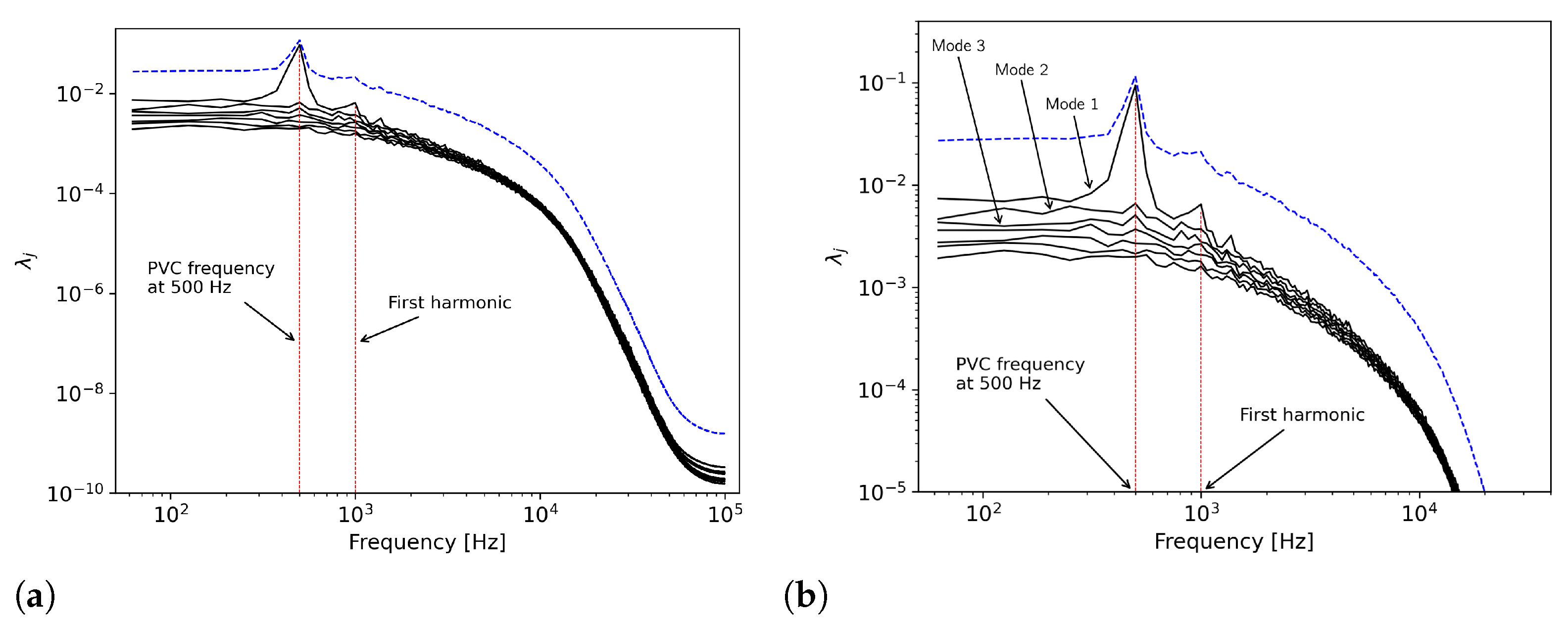
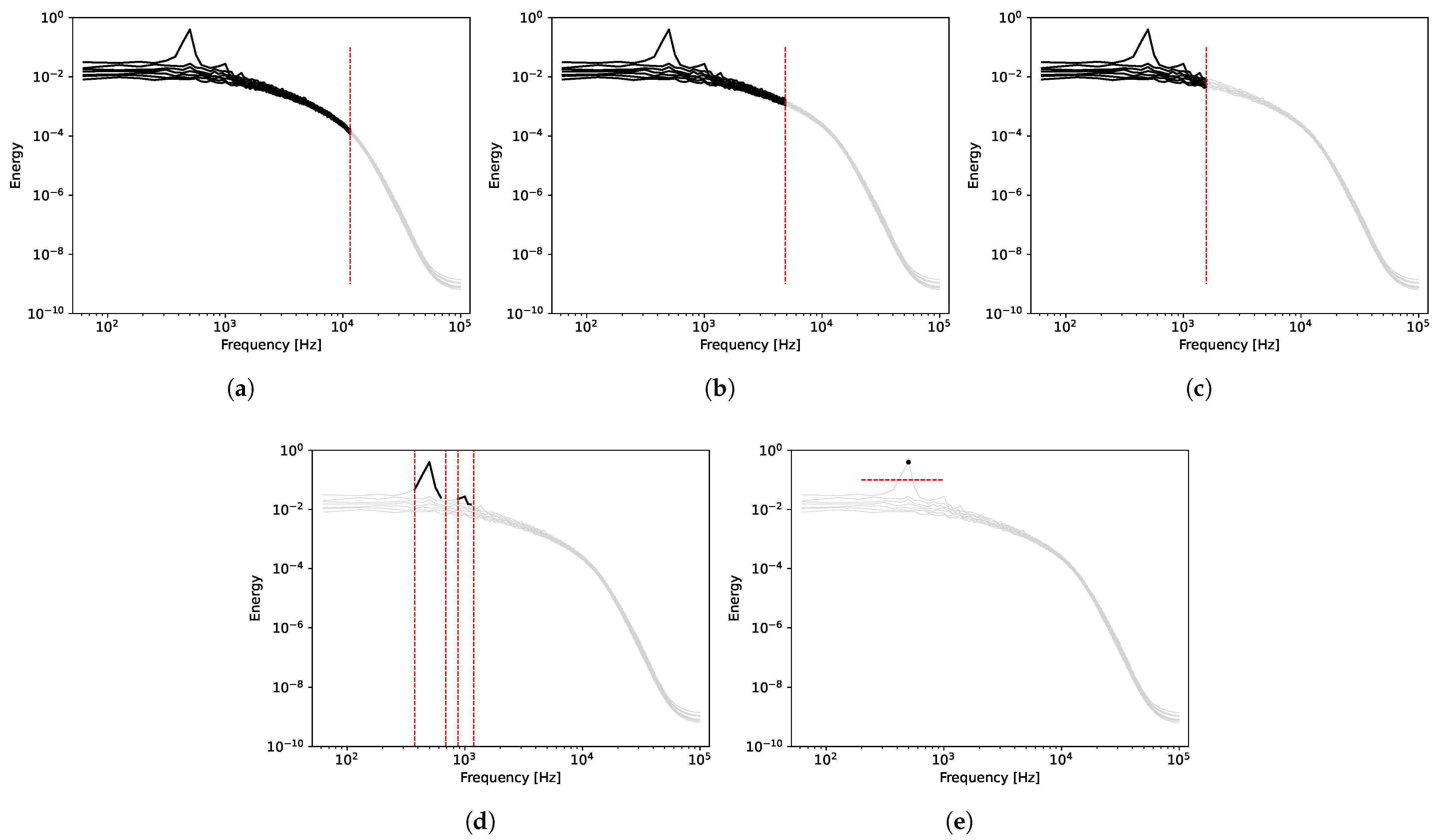
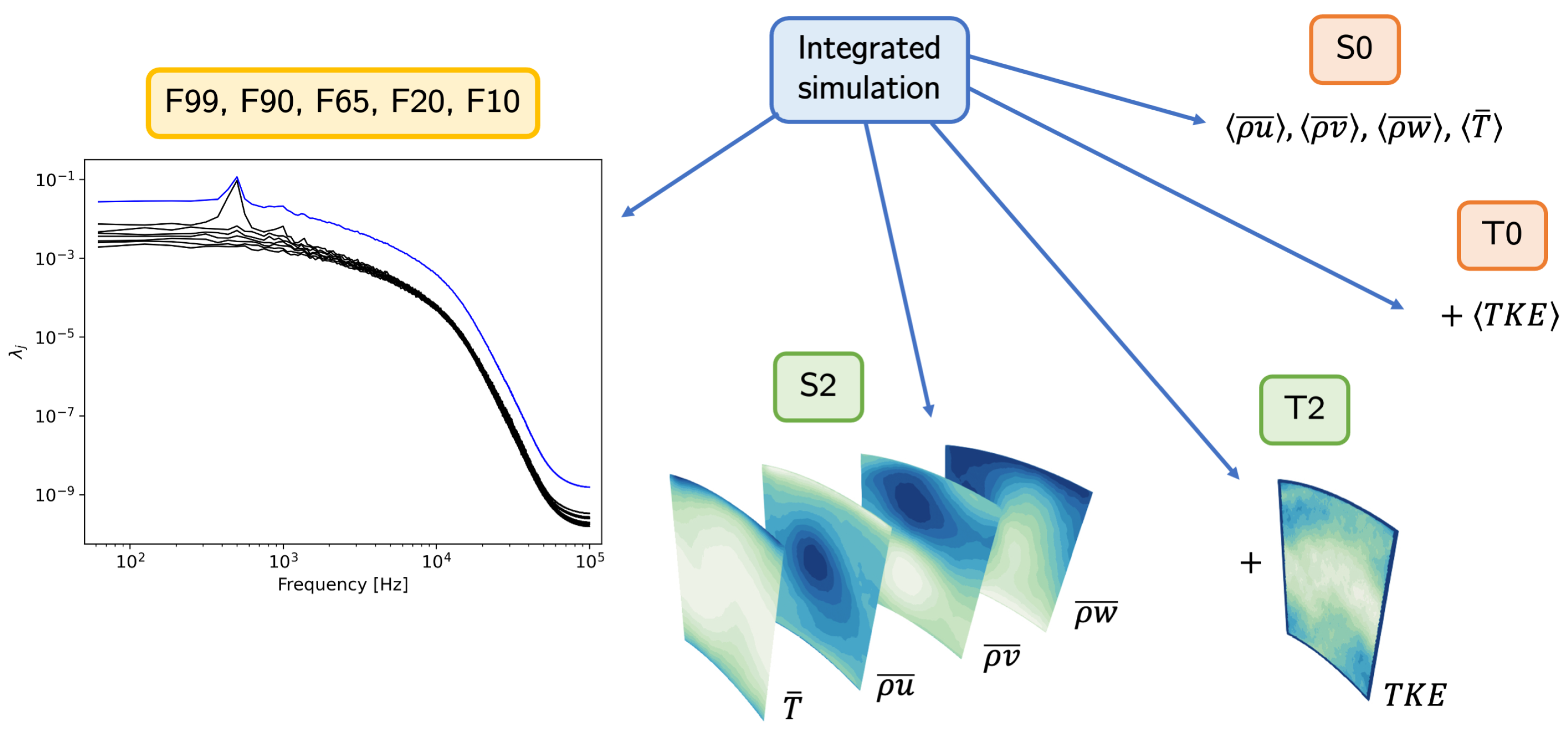
The SPOD spectrum obtained with these parameters contains a total of seven modes and is presented in Figure 5. The eigenvalues are normalized by the sum of the total energy on all the frequencies and modes. The blue line corresponds to the power spectral density which is reconstructed by summing the energies of each mode for all the frequencies of the spectrum. Mode 1 clearly evidences the frequency of the PVC at 500 Hz, as well as its first harmonic at 1000 Hz.

At a given frequency, the presence of a significant shift in terms of energy between the first mode and the following modes shows that the modal decomposition is low order, that is to say that the physical phenomenon of this frequency is very well described by the first mode, and the latter dominates the dynamics of the flow. This is mainly the case for the frequency at 500 Hz and for its first harmonic at 1000 Hz. To demonstrate this property of the flow, Figure 6 plots the eigenvalues at 500 Hz and 1000 Hz as a function of the seven modes, normalized by the total energy at each frequency. It corresponds to the evolution of ${\lambda }_i$ along the two dashed red lines of Figure 5 at frequencies 500 Hz and 1000 Hz. It is clear that at 500 Hz, mode 1 is significantly more energetic than the others since it captures about 80% of the total energy at this frequency. Likewise, this effect is also present at 1000 Hz, where the dominant mode 1 captures more than 30% of the energy.

Moreover, in the SPOD spectrum, the presence of a peak at 500 Hz for the first mode dominating the overall energy level shows that the flow at the chamber/turbine interface is mainly driven by the PVC, which generates high activity at this frequency. On the contrary, when the difference between the eigenvalues of the modes is not significant (here for most frequencies, with the exception of the frequency of the PVC and its harmonics), it means that a single mode is not capable of describing the flow physics. This is, for example, the case for high frequencies, associated with flow turbulence. To describe the physics of the flow at these frequencies, we must instead consider the SPOD modes as a basis of eigenvectors of comparable importance. This behavior can be easily understood, turbulence being a rather random phenomenon, it cannot be described by a unique mode for the corresponding frequencies.

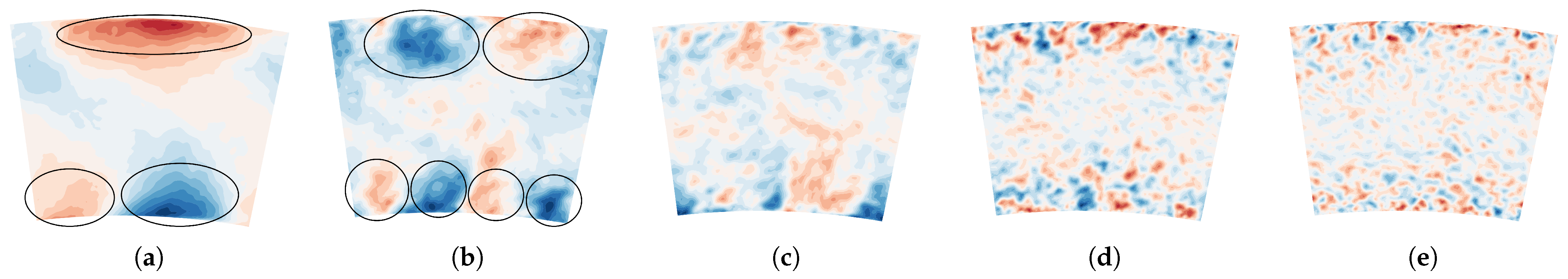
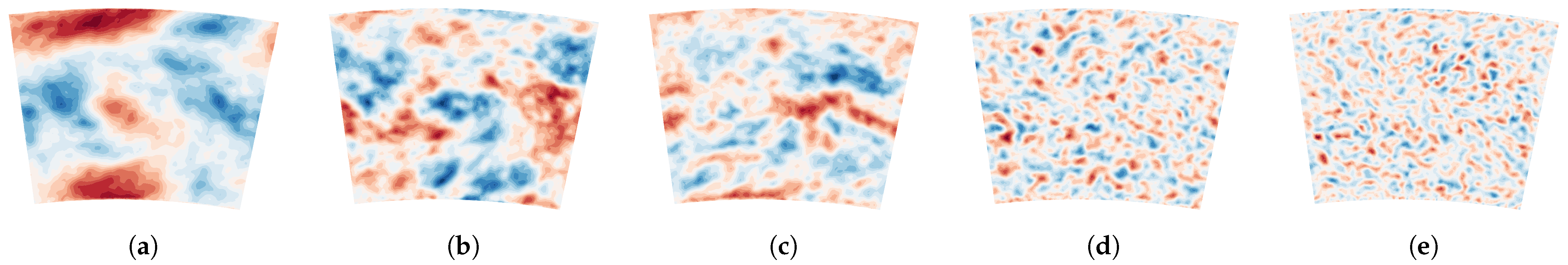
To learn more about the flow topology using the SPOD decomposition, the spatial representation of the first mode for different frequencies is analyzed. The spatial modes of temperature are shown in Figure 7. At 500 Hz, the first mode clearly shows one lobe at the inner wall and two lobes at the outer wall, in phase opposition. These modes result from the excitation of the flow injected through the multiperforations by the PVC frequency. At 1000 Hz, the same phenomenon is observed, with a doubling of the number of lobes (two external and four internal lobes). For these two frequencies, as explained previously, the first mode is largely dominant in terms of energy compared to the following modes. The dynamics of the flow at these two frequencies is therefore mainly driven by the spatial shape of mode 1. For frequencies between 1500 Hz and 8000 Hz, a progressive decrease in the structure size is observed. This can be explained simply by the fact that smaller structures in the flow are governed by smaller time scales (and thus higher frequencies). To continue the analysis, the spatial representation of the same frequencies for the axial velocity is given in Figure 8. This time, the flow activity at 500 Hz and 1000 Hz is not restricted to the near-wall region; it extends over the entire height of the channel. This behavior is again related to the PVC. Unlike the temperature, which is rather homogeneous in the channel center, as the injection temperature of the hot flow is constant, the velocity varies at the outlet of the injector due to the swirling motion introduced by the PVC. Therefore, the spatial structures of the modes at these frequencies also extend to the center of the channel. For frequencies between 1500 Hz and 8000 Hz, the observations are similar to those made for temperature. The structures are very homogeneous and the size of the structures decreases as the mode frequency increases.

The use of SPOD to analyze the database of snapshots at the chamber/turbine interface clearly demonstrated its capability to identify the main flow dynamics in terms of frequencies. What follows is the same analysis using proper orthogonal decomposition in order to underline the benefits of SPOD for the considered configuration.

2.2.2. Modal Decomposition 2: Proper Orthogonal Decomposition (POD)

POD was introduced by Lumley [6,37] for the analysis of turbulent flows. In practice, POD enables the reduction of an initial database of high dimension to another of lower dimension. The purpose of the method is to determine a base of orthogonal spatial modes, which facilitates the identification of coherent structures in the flow with the objective of producing a reduced model of the initial database. A detailed comparison between the different methods of modal decompositions is made in [8]. In short, POD provides a base of coherent eigenmodes in space only. The method is therefore not capable of highlighting the temporal correlations which may exist within the database. However, temporal coherence is a very present phenomenon in most flows containing large coherent structures.

In practice, the eigenmodes of POD are composed of coherent structures coming from different frequencies. This results in a wide-frequency spectrum for the temporal coefficients, as demonstrated later. This combination of frequencies for the eigenmodes means that each eigenmode mixes flow physical phenomena of different time scales. As a consequence, it is more difficult to extract and analyze the contribution of different coherent flow structures.

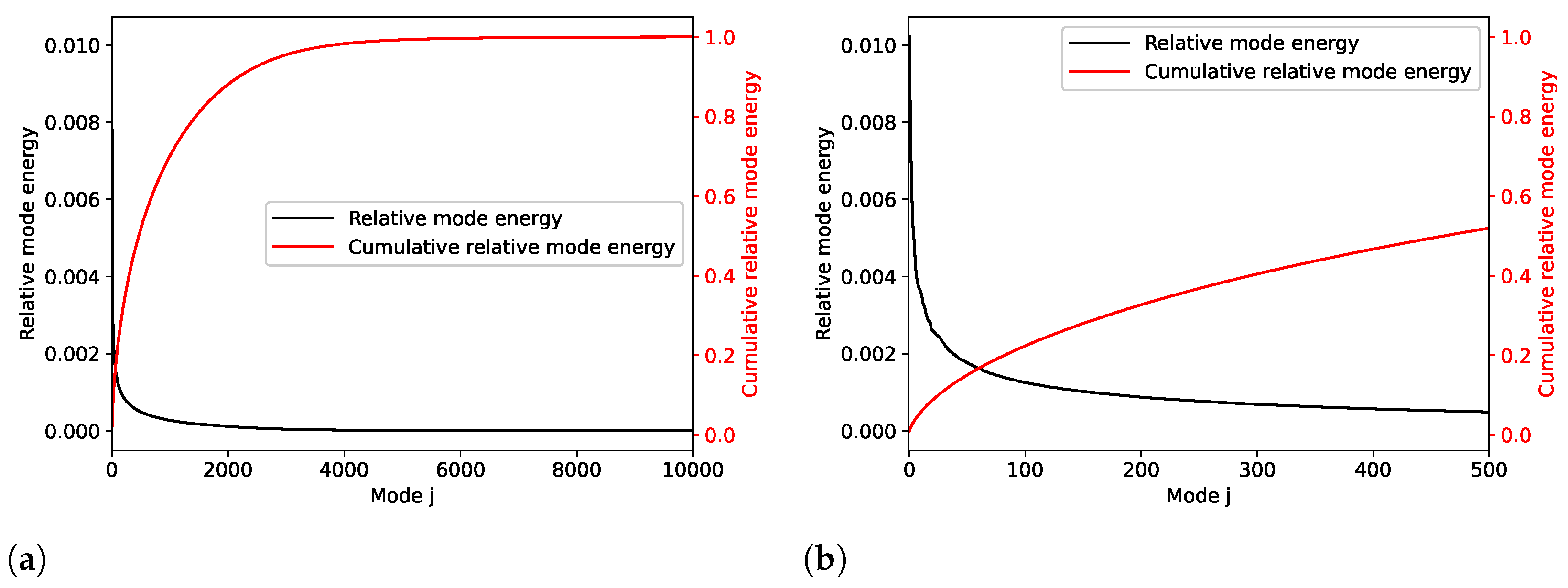
To illustrate the previous remarks, a POD decomposition is performed on the initial numerical database with $\mathbf{q}=[{\rho }^{\prime },u^{\prime },v^{\prime },w^{\prime },T^{\prime }]$ (for reasons of memory capacity, only 10,000 snapshots are used instead of the 20,000 available in the full numerical database). The analysis of the 10,000 eigenvalues of the modal decomposition shows that the decrease in terms of energy is very slow (Figure 9). About 2200 modes are needed to capture 90% of the total energy and over 4600 modes to recover 99% of the total energy. This highlights the fact that POD has difficulty producing a reduced model of the original database.

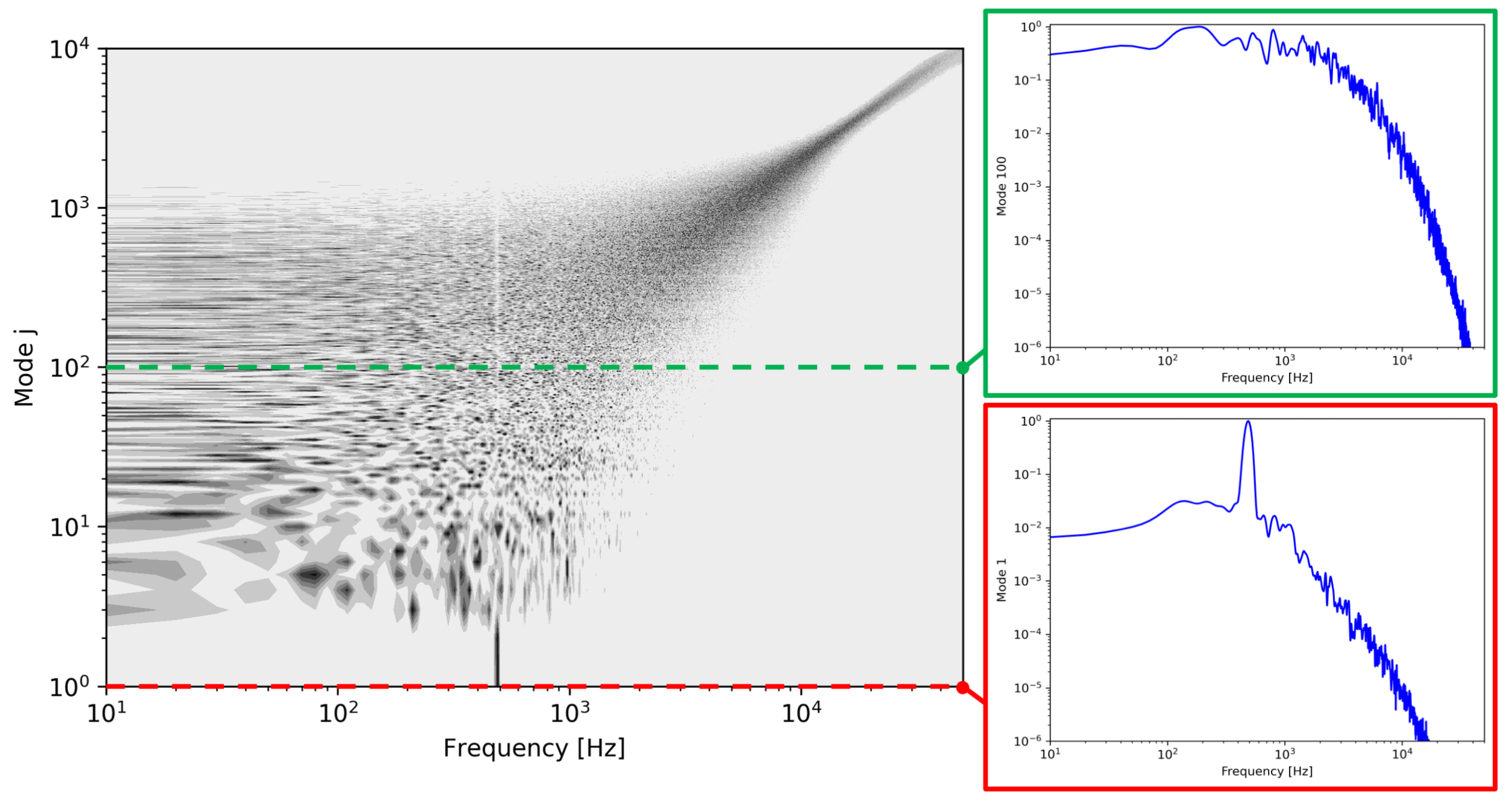
Another interesting illustration is given in Figure 10. It represents the power spectral density of each POD temporal coefficient with contour normalized by the maximum value of its power spectral density (PSD). For a given mode j, this means that for a given frequency along the x-axis, the darker the color, the closer its level is to the PSD maximum of the POD temporal coefficient of mode j. For example, the red dashed line associated with mode 1 shows that its temporal coefficient mainly contained the frequency associated with the PVC at 500 Hz. This is also the case for mode 2. On the contrary, for the rest of the modes, the large number of frequencies are close to the maximum of the power spectral density. The second plot shows the PSD of mode 100 located along the green dashed line. It is clear that no frequency dominates over the others. This representation highlights the preceding remark: the temporal coefficients of the eigenmodes obtained by POD contain a wide range of frequencies and the associated modes thus represent a behavior of the flow which combine several time scales, which was not the case for the SPOD.

3. Generation of an Unsteady Inlet Boundary Condition for an Isolated Turbine Simulation

The two previous modal decompositions enabled learning more about the dynamics of the flow at the interface between the combustion chamber and the turbine. SPOD is also shown to be particularly effective in identifying dominant structures in flow physics by highlighting the dynamics associated with PVC. The objective of this section is hence the use of SPOD to build various unsteady boundary conditions, accounting for the coupling of the turbine with the chamber, while compressing the size of the initial database. The idea is to construct and compare different types of inflow signals for an isolated turbine simulation to understand the impact of the required degree of information needed for such LES. The configuration used is shown in Figure 11. It simply corresponds to the integrated simulation domain reduced to the turbine.

As explained in the previous section, it is possible to perform partial reconstructions of the initial database based on SPOD. The choice of the reconstruction cannot, however, be totally arbitrary, and different characteristics are targeted in the following cases. To do so, five partial reconstructions are performed with different levels of total energy,

• Case F99 corresponds to a reconstruction containing 99% of the total energy, with all seven identified modes and the first 185 frequencies which extend to 11,500 Hz.
• Case F90 corresponds to a reconstruction containing 90% of the total energy, with, again, the seven modes and the first 79 frequencies which extend to 5000 Hz.
• Case F65 corresponds to a reconstruction containing 65% of the total energy, with the seven modes and the first 26 frequencies which extend to 1500 Hz.
• Case F20 corresponds to a reconstruction containing 20% of the total energy, with only the first mode and the frequencies around 500 Hz, as well as the first harmonic at 1000 Hz.
• Case F10 corresponds to a reconstruction containing 10% of the total energy, with only the first mode and the dominant frequency at 500 Hz (Figure 12).

Figure 12. SPOD spectra of the partial reconstructions. (a) F99. (b) F90. (c) F65. (d) F20. (e) F10.

Figure 12. SPOD spectra of the partial reconstructions. (a) F99. (b) F90. (c) F65. (d) F20. (e) F10.

The position of the thresholds in the SPOD spectrum is presented for each case in Figure 12.

The exact characteristics of the different SPOD reconstructions are presented in

Table 2. Details of each reconstruction and the storage cost relative to the initial database.

Case	Number of Frequencies	Number of Modes	Total Energy of the Reconstruction	Storage Cost of the Reconstruction Relative to the Initial Database
F99	185	7	98.99%	6.5%
F90	79	7	90.03%	2.8%
F65	26	7	64.58%	0.9%
F20	10	1	18.35%	0.05%
F10	1	1	9.37%	0.005%

. The last column of the table contains additional information: the cost of storing the corresponding information. The main idea of the partial reconstruction of the database is to provide a boundary condition signal which best replicates the coupling between the chamber and the turbine while using a smaller database than the set of initial snapshots. This storage cost is expressed relative to the size of the initial database.

The five cases of Table 2 take advantage of SPOD to generate the unsteady boundary condition. These are furthermore compared to four other cases which use traditional methods:

• Case S0: the inlet boundary condition is imposed by specifying 0D quantities in space and time, i.e., by imposing the three components of momentum $\rho u$, $\rho v$, and $\rho w$ and the static temperature (spatially and temporally averaged values of the integrated simulation).
• Case T0: the quantities imposed at the inlet are the same as for case S0, with the addition of velocity fluctuations generated randomly to create turbulent activity in space and time. Turbulence is injected here using the synthetic approach proposed by Guezennec et al. [38] from a Passot–Pouquet spectrum [39]. The velocity fluctuation value used comes from the integrated simulation and the most energetic length scale is specified at ${\lambda }_e=h/4$, with h the height of the channel. This quantity corresponds to the characteristic size of the most energetic structures of the Passot–Pouquet spectrum [39] (not to be confused with the integral scale ${\mathsf{\Lambda }}_f$ which is expressed as ${\mathsf{\Lambda }}_f={\lambda }_e/\sqrt{2\pi }$).
• Case S2: the inlet boundary condition is imposed from time-averaged 2D maps at the interface of the integrated simulation for $\rho u$, $\rho v$, $\rho w$, and T. The boundary condition condition is therefore constant in time, but variable in space.
• Case T2: this case is identical to S2 with the addition of a 2D map of velocity fluctuations. The turbulent 2D field coincides with the turbulent kinetic energy at the interface of the integrated simulation, i.e., time-averaged fluctuating field. Unlike the T0 case, the value of the velocity fluctuations used to generate the synthetic turbulence is hence not constant in space. Note that the turbulence injection method does not inject fluctuations on temperature.

All available cases are summarized in Figure 13.

Analysis of the Reconstructed Fields

To give a better idea of the characteristics of the signals imposed for cases F99, F90, F65, F20, and F10, Figure 14 plots the evolution of the spatial average of the static temperature at the inlet plane obtained by reconstructions behind the five cases compared to the reference case (the initial database) for a period of 0.005 s. The frequency cutoff of the SPOD spectrum is, here, clearly visible in each case. It is also clear that case F99 very well reproduces the rapid changes in temperature seen in the reference. For case F90, the global trend is respected, but the rapid variations (which are therefore at high frequencies) are smoothed out. This behavior is even more marked for F65. For cases F20 and F10, whose reconstruction contains only a limited number of frequencies, the evolution is as expected even more simplified. Finally, for case F10, only the oscillation at the 500 Hz frequency is present.

The previous figures have given an overview of the type of signal imposed by the unsteady boundary conditions of cases F99 to F10. The following aims at giving a more quantitative analysis in the spectral domain. To do so, Figure 15 presents the power spectral densities (PSD) of the axial velocity for the cases F99 to F10 for a probe located at the center of the inlet plane (at mid-height of the vein and at an angle of $8^{\circ }$). Analysis of the PSD coming directly from the reconstructed database (before the application of the boundary condition) clearly shows the introduced cut-off frequencies for the different cases, as described in Figure 12. It is accordingly observed that beyond the respective cut-off frequencies of each case, the energy levels are zero.

By performing a PSD of the signal from the isolated simulations on a probe located at plane 40 (located just after the inlet plane), the observations are different (Figure 16). For cases F99 and F90, the cutoff frequency is no longer visible. This is explained by the fact that the cutoff frequency for these two cases is located at the end of the inertial zone and in the dissipative region of the energy cascade, respectively. Therefore, in both cases, the beginning of the energy cascade is present in the specified inlet fields and only a small part of the turbulence has to be regenerated. This specific process is well captured here, and the spectrum is rapidly and correctly regenerated. For case F65, which has a cutoff frequency at the beginning of the inertial zone, this is no longer the case. There is an energy transfer between the large and small scales but the energy level of the small scales no longer matches the reference. Finally, for cases F20 and F10, whose reconstruction is composed of a band-pass filter around 500 Hz and 1000 Hz, or only of the frequency 500 Hz, respectively, the spectrum at plane 40 is very different from the reference. Their respective spectra mainly highlight the multiple harmonics of the retained frequencies, and turbulence is not yet properly recovered.

Finally, and in order to illustrate the impact of the injected signals on the full LES predicted flow field, the static temperature distribution for all the nodes of plane 40 and for the 20,000 snapshots of the database is given in Figure 17. For the reference, as well as for cases F99 and F90, a peak is observed at 300 K which corresponds to the injection temperature of the cold flow by the multiperforations. At the chamber/turbine interface, these extreme temperature values are still visible. The second peak is located at a value around 513 K (injection temperature of the hot flow of the plenum). For F65, the peak at 300 K is hardly visible, and even disappears completely for cases F20 and F10. This is simply due to the fact that the fluctuations imposed at the inlet are no longer sufficiently large to consider and capture this extremum. As the reconstruction becomes more and more incomplete, the width of the temperature distribution is reduced and the extreme values are no longer reached by the boundary condition [40].

4. Effects of the Boundary Condition of the Isolated Simulation Predictions

The first step to evaluate the different inlet boundary conditions and their impact on the flow predicted by the isolated simulations is to compare their 0D quantities. The analyzed quantities are presented in

Table 3. Comparison of the reduced mass flow rate $Q_r=\frac{Q\sqrt{R{T}_t^{40}}}{P_t^{40}{L}^2}$ (where Q is the mass flow rate, R is the perfect gas constant, and L is the radius at mid-vein height) and the ratios of total pressure and temperature between plane 40 and the outlet. The reference corresponds to the integrated combustor/turbine simulation.

	${\mathit{Q}}_{\mathit{r}}$	${\mathit{P}}_{\mathit{t}}^{40}/{\mathit{P}}_{\mathit{t}}^{\mathbf{Out}}$	${\mathit{T}}_{\mathit{t}}^{40}/{\mathit{T}}_{\mathit{t}}^{\mathbf{Out}}$
Ref.	0.0868	1.122	1.034
F99	0.0868	1.122	1.034
F90	0.0868	1.122	1.034
F65	0.0868	1.122	1.034
F20	0.0868	1.121	1.034
F10	0.0868	1.120	1.034
S0	0.0871	1.112	1.022
T0	0.0867	1.119	1.024
S2	0.0867	1.119	1.028
T2	0.0865	1.120	1.032

. The second column contains the reduced mass flow rate $Q_r=Q\sqrt{R{T}_t^{40}}/\left(P_t^{40}{L}^2\right)$, where L is the radius at mid-vein height. The third and fourth columns compare the total pressure and temperature ratios between the plane 40 and the domain exit. The exact position of the planes is given in Figure 11. Note that the quantities are spatially and temporally averaged in each plane. This comparison is done to verify that the choice of the inlet boundary condition does not affect the simulated operating point. A change in the operating point could indeed distort the comparison of the different cases. From the compared quantities, it is clear that each operating point remains very close to the reference integrated simulation. The relative difference of reduced mass flow rate compared to the reference remains below 0.2% for all cases. For the total pressure and temperature ratios, the SPOD cases are almost identical to the reference. For the standard boundary conditions, some differences are observed. In particular, the total temperature ratio is slightly lower for the cases S0, T0, and S2. This difference can be explained by the difference in flow properties. In particular, for the cases S0 and S2, which use stationary inlet boundary conditions, the turbulent activity is less pronounced than for the reference. This lower turbulent activity may reduce the overall losses in the domain and, thus, the total temperature ratio [41].

4.1. Turbulent Fluctuations

To better quantify the differences introduced by the choice of the different inlet signals regarding the turbulent activity of the various simulations, the turbulent kinetic energy (TKE), the RMS fluctuations of the three components of velocity, and total temperature, as well as the turbulent intensity spatially averaged in planes 40 (before the vane) and 41 (after the vane), are compared for each case (

Table 4. Spatial average of TKE, velocity RMS, total temperature RMS, and turbulent intensity at plane 40. The color of the values are determined by their relative difference compared to the reference: Green for relative differences lower than 5%, orange between 5% and 20%, and red for relative differences greater than 20%. The reference corresponds to the integrated combustor/turbine simulation.

	$\langle \overline{\mathbf{TKE}}\rangle$	$\langle \overline{{\mathit{u}}_{\mathbf{rms}}}\rangle$	$\langle \overline{{\mathit{v}}_{\mathbf{rms}}}\rangle$	$\langle \overline{{\mathit{w}}_{\mathbf{rms}}}\rangle$	$\langle \overline{{\mathit{I}}_{\mathbf{u}}}\rangle$	$\langle \overline{{\mathit{T}}_{\mathit{t},\mathbf{rms}}}\rangle$
	$\left[{\mathrm{m}}^2·{\mathrm{s}}^{-\mathbf{2}}\right]$	$\left[\mathrm{m}·{\mathrm{s}}^{-\mathbf{1}}\right]$	$\left[\mathrm{m}·{\mathrm{s}}^{-\mathbf{1}}\right]$	$\left[\mathrm{m}·{\mathrm{s}}^{-\mathbf{1}}\right]$	$[\%]$	$\left[\mathrm{K}\right]$
Ref.	323.04	12.91	15.38	14.97	29.66	33.01
F99	321.4	12.86	15.35	14.92	29.58	33.05
F90	322.08	12.81	15.41	14.89	29.6	33.32
F65	259.39	11.21	14.15	13.01	26.46	31.59
F20	100.04	6.75	9.09	7.6	16.55	20.72
F10	38.19	3.4	5.69	4.03	10.05	12.11
S0	2.77	0.96	1.33	1.02	2.54	2.22
T0	321.72	14.25	14.92	14.45	31.47	3.04
S2	2.31	0.96	1.08	1.0	2.4	2.1
T2	327.55	14.38	14.96	14.37	29.71	11.11

and

Table 5. Spatial average of TKE, velocity RMS, total temperature RMS, and turbulent intensity at plane 41. The color of the values are determined by their relative difference compared to the reference: Green for relative differences lower than 5%, orange between 5% and 20%, and red for relative differences greater than 20%. The reference corresponds to the integrated combustor/turbine simulation.

	$\langle \overline{\mathbf{TKE}}\rangle$	$\langle \overline{{\mathit{u}}_{\mathbf{rms}}}\rangle$	$\langle \overline{{\mathit{v}}_{\mathbf{rms}}}\rangle$	$\langle \overline{{\mathit{w}}_{\mathbf{rms}}}\rangle$	$\langle \overline{{\mathit{I}}_{\mathbf{u}}}\rangle$	$\langle \overline{{\mathit{T}}_{\mathit{t},\mathbf{rms}}}\rangle$
	$\left[{\mathrm{m}}^2·{\mathrm{s}}^{-\mathbf{2}}\right]$	$\left[\mathrm{m}·{\mathrm{s}}^{-\mathbf{1}}\right]$	$\left[\mathrm{m}·{\mathrm{s}}^{-\mathbf{1}}\right]$	$\left[\mathrm{m}·{\mathrm{s}}^{-\mathbf{1}}\right]$	$[\%]$	$\left[\mathrm{K}\right]$
Ref.	629.74	18.8	19.96	18.43	5.92	22.81
F99	631.79	18.84	19.96	18.48	5.92	22.77
F90	647.87	19.16	20.14	18.79	6.0	22.92
F65	681.92	19.62	20.6	19.45	6.17	24.7
F20	487.03	15.46	18.09	15.09	5.1	22.74
F10	342.86	11.53	15.36	11.09	4.12	18.2
S0	194.93	6.73	9.97	5.53	2.62	4.95
T0	520.47	17.57	16.74	16.45	5.41	10.16
S2	193.87	7.1	10.42	6.32	2.79	6.34
T2	575.65	18.54	18.25	17.58	5.72	14.53

).

Given that plane 40 is located directly downstream of the entry plane, the properties obtained for this plane are almost exclusively induced by the prescribed inlet field (Table 4). For cases F99 and F90, for which a large part of the energy of the fluctuations is preserved by their reconstructions (respectively 99% and 90%), the values obtained are very comparable to the reference values. When the reconstruction contains a smaller part of the energy distribution, the fluctuating fields gradually decrease (case F65, F20, and F10). Not surprisingly, cases S0 and S2, without synthetic turbulence injection, have fluctuation levels close to zero.

Finally, for cases T0 and T2, one notes that the values of TKE at plane 40 are very close to the reference, as this value was used to define the parameters of the synthetic turbulence injection. However, since the method uses homogeneous and isotropic turbulence, the fluctuations of the three velocity components are, by construction, comparable. Nevertheless, and unlike the reference which has a certain anisotropy of fluctuations with $\langle \overline{v_{\mathrm{rms}}}\rangle /\langle \overline{u_{\mathrm{rms}}}\rangle \simeq 1.16$ and $\langle \overline{w_{\mathrm{rms}}}\rangle /\langle \overline{u_{\mathrm{rms}}}\rangle \simeq 1.17$, this feature is absent here. Moreover, and because the injection method is not able to inject temperature fluctuations on top of velocity fluctuations, the RMS of the total temperature remains very low.

To delve further in the comparison between the flow turbulent properties of the different cases, the data of each node located on plane 40 are plotted in a turbulence triangle [42]. This representation is shown in Figure 18 for cases F99, F65, T0, and T2. To facilitate the understanding of such analysis, three triangles are plotted for each case. The first one contains every node of plane 40 (noted full). The second one contains only the nodes located in the center of the vein (between 25% and 75% of the total channel height). The third one contains the nodes in the upper and lower near-wall regions (lower than 1% and greater than 99% of the total channel height, respectively). When comparing F99 and F65, it is clear that despite the difference in RMS values observed in Table 4, the turbulent properties are similar, particularly in the channel center where the turbulence is not isotropic. Close to the walls, the nodes are mainly located in the two-component region of the triangle, as the turbulent fluctuation normal to the wall is much lower compared to the two remaining components. On the contrary, for T0 and T2, the turbulence in the channel center is mainly isotropic, which is again linked to the properties of the injection method.

Downstream of the vane, i.e., at plane 41, for the SPOD cases, observations are similar (Table 5). The cases using a large part of the energy in the reconstructions have values very close to the reference. Likewise, the cases without turbulence injection have very low fluctuation values. Note that for the cases T0 and T2, although the levels of TKE in plane 40 are identical to the reference, levels at plane 41 are significantly lower than the reference. As for plane 40, the turbulence triangles of F99, F65, T0, and T2 are shown in Figure 19. For F99 and F65, from the values given in Table 5, one could think that the turbulence had become isotropic after the vane. However, the turbulence triangles for the nodes located in the channel center show that it is not the case. The nodes remain far from the lower corner of the triangle which corresponds to isotropic turbulence. For cases T0 and T2, the turbulence properties are close, despite the lower level of turbulence intensity.

4.2. Adiabatic Wall Temperature

In the development of a turbine stage, the aerodynamic properties of the flow field is relevant, but thermics plays also a preponderant role for the thermal integrity of the vane. This is why it is important to focus on the adiabatic wall temperature and the effect of the inflow specification on this quantity. For our specific problem, since the hot spot directly impacts blade #2, it is the most thermally exposed to the high temperatures of the chamber. This justifies why the following analysis focuses only on blade #2.

With the objective of analyzing the blade thermics, the mean adiabatic temperature contours at the blade wall #2 for the compared cases are presented in Figure 20. Except for the S2 case, the contours of the other cases are very close. A high-temperature region is visible at the leading edge of the blade, indicative of the interaction between the hot spot with the blade. The effectiveness of the cooling film is also highlighted. The temperature level is much lower downstream of the holes than upstream. The contours also show a flow deviation related to the swirl. For the S2 case, the temperature at the leading edge is greatly overestimated due to the lack of turbulent mixing introduced by the boundary condition. Thus, the hot spot generated by the chamber is not dissipated between the entry plane and the leading edge. No significant difference is to be reported for the cases F90 and F65 compared to the reference integrated simulation.

To complete the previous analysis made on 2D contours, Figure 21 presents the evolution of the average adiabatic wall temperature (temporal average and averaged along the radial direction) along the curvilinear abscissa of the blade as obtained from the various simulations. Added to the figures are the minimum and maximum values reached at each coordinate of the curvilinear abscissa. For case F90, the agreement with the reference is excellent for the average, the minimum, and the maximum values. The maximum adiabatic temperature variation, with a maximum around 450 K at the leading edge, confirms the direct interaction of the blade with the hot spot, despite cooling. For case F65, the comparison with the reference is also very satisfactory. Only the maximum temperature is slightly underestimated (by about 5 K over the entire length of the curvilinear abscissa). For case S2, without turbulence injection, the results are clearly not satisfactory. The average temperature profile does not match the reference and the maximum temperature is greatly overestimated. Finally, case T2 produces rather interesting results. The average and minimum profiles agree well with the reference. However, the maximum temperature profile yields poorer results. The maximum temperature is sometimes underestimated by more than 15 K along the curvilinear abscissa, which can be critical for the life duration estimation of a turbine.

5. Conclusions

The objective of the study was to highlight the capacity of generating realistic inflow conditions that are unsteady, turbulent, and capable of replicating the multicomponent coupling in the case of an isolated turbine LES. The results show that a numerical database consisting of snapshots of the flow recorded at the interface between the combustion chamber and the turbine of an integrated simulation can be used to construct realistic inflow conditions, taking into account the velocity and temperature fluctuations naturally present in the coupled simulation. The recorded numerical database is first analyzed by means of two modal decomposition methods to evaluate such approaches and their impact on the reconstruction process. The SPOD method proves to be very interesting in that respect as it allows analysis of the global dynamics of the flow and highlighting of the predominant structures of the flow in space and frequency, contrarily to POD. Following this modal decomposition carried out in the frequency domain, it is possible to generate several partial reconstructions of the initial numerical database. These reconstructions are then used at the inlet plane of the isolated turbine LES domain to build realistic and unsteady inflow conditions.

Thanks to the spectral representation of SPOD, it is shown that if the reconstruction conserves a sufficient part of the total turbulent energy (at least 65%), the reconstructed condition yields LES predictions that are very comparable to the integrated reference simulation, unlike conditions relying on synthetic turbulence injection methods. The SPOD reconstruction is, furthermore, able to inject fluctuations for both velocity and temperature. This specificity is observed to be of paramount importance to recover the correct temperatures and levels of temperature fluctuations on the surface of the blades.

This represents an undeniable advantage compared to synthetic turbulence injection methods which are generally failing on this precise point. The study also shows that standard boundary conditions relying on 0D quantities or 2D maps, with or without synthetic turbulence injection, do not allow capture of the coupling between the combustion chamber and the turbine. This is especially true on this configuration, for which the PVC plays a strong role in the overall flow structure in the chamber and, as a result, at the chamber/turbine interface. In some cases, and with these simplified approaches, when the boundary condition parameters are precisely defined, it is possible to obtain velocity fluctuation levels in agreement with the reference simulation at the inflow. However, due to the turbulence injection method used, the temperature fluctuations are always too low for these standard boundary conditions.

To conclude, only one configuration was used here, where the injector is aligned with the leading edge of blade #2. One idea would be to use the same numerical database and the same partial reconstructions to perform isolated simulations with a different alignment of the blades with respect to the injector. The modification of the alignment would enable evaluation of whether the numerical database and the realistic boundary conditions are able to accurately reproduce the chamber/turbine coupling, despite the configuration modification. This perspective is part of a design office logic during the development of turbine geometries. Indeed, during this phase of development, many iterations are made on the geometry and the dimensions of the blades. The proposed method could thus allow us to carry one integrated simulation or an isolated simulation of the chamber to generate a numerical database from the simulation and then generate partial reconstructions, taking into account the dominant properties of the flow. From these available realistic boundary conditions, the different geometries could be analyzed in the case of an isolated domain while taking into account the effect of the chamber at the entry plane for a reduced cost.

References

1. Medic, G.; Kalitzin, G.; You, D.; Herrmann, M.; Ham, F.; Weide, E.; Pitsch, H.; Alonso, J. Integrated RANS/LES computations of turbulent flow through a turbofan jet engine. Annu. Res. Briefs 2006, 275–285. Available online: https://web.stanford.edu/group/ctr/ResBriefs06/21_medic1.pdf (accessed on 2 December 2021).
2. Medic, G.; You, D.; Kalitzin, G.; Herrmann, M.; Ham, F.; Pitsch, H.; van der Weide, E.; Alonso, J. Integrated Computations of an Entire Jet Engine. In Proceedings of the ASME Turbo Expo 2007: Power for Land, Sea, and Air, Montreal, QC, Canada, 14–17 May 2007; Volume 6, pp. 1841–1847. [Google Scholar] [CrossRef]
3. Pérez Arroyo, C.; Dombard, J.; Duchaine, F.; Gicquel, L.; Martin, B.; Odier, N.; Staffelbach, G. Towards the large-eddy simulation of a full engine: Integration of a 360 azimuthal degrees fan, compressor and combustion chamber. Part I: Methodology and initialisation. J. Glob. Power Propuls. Soc. 2021, 2021, 1–12. [Google Scholar] [CrossRef]
4. Pérez Arroyo, C.; Dombard, J.; Duchaine, F.; Gicquel, L.; Martin, B.; Odier, N.; Staffelbach, G. Towards the large-eddy simulation of a full engine: Integration of a 360 azimuthal degrees fan, compressor and combustion chamber. Part II: Comparison against stand-alone simulations. J. Glob. Power Propuls. Soc. 2021, 2021, 1–16. [Google Scholar] [CrossRef]
5. Duchaine, F.; Dombard, J.; Gicquel, L.; Koupper, C. On the importance of inlet boundary conditions for aerothermal predictions of turbine stages with large eddy simulation. Comput. Fluids 2017, 154, 60–73. [Google Scholar] [CrossRef]
6. Lumley, J.L. Stochastic Tools in Turbulence; Academic Press: Cambridge, MA, USA, 1970. [Google Scholar]
7. Sirovich, L. Turbulence and the dynamics of coherent structures. I—Coherent structures. II—Symmetries and transformations. III—Dynamics and scaling. Q. Appl. Math. 1987, 45, 561–571. [Google Scholar] [CrossRef] [Green Version]
8. Towne, A.; Schmidt, O.T.; Colonius, T. Spectral proper orthogonal decomposition and its relationship to dynamic mode decomposition and resolvent analysis. J. Fluid Mech. 2018, 847, 821–867. [Google Scholar] [CrossRef] [Green Version]
9. Ghate, A.S.; Towne, A.; Lele, S.K. Broadband reconstruction of inhomogeneous turbulence using spectral proper orthogonal decomposition and Gabor modes. J. Fluid Mech. 2020, 888, R1. [Google Scholar] [CrossRef]
10. Bacci, T.; Caciolli, G.; Facchini, B.; Tarchi, L.; Koupper, C.; Champion, J.L. Flowfield and Temperature Profiles Measurements on a Combustor Simulator Dedicated to Hot Streaks Generation. In Proceedings of the ASME Turbo Expo 2015: Turbine Technical Conference and Exposition, Montreal, QC, Canada, 15–19 June 2015; Volume 5C. [Google Scholar] [CrossRef]
11. Krumme, A.; Tegeler, M.; Gattermann, S. Design, integration and operation of a rotating combustor-turbine-interaction test rig within the scope of the EC FP7 Project FACTOR. In Proceedings of the 13th European Conference on Turbomachinery Fluid Dynamics & Thermodynamics, Lausanne, Switzerland, 8–12 April 2019. [Google Scholar]
12. Adams, M.G.; Beard, P.F.; Stokes, M.R.; Wallin, F.; Chana, K.S.; Povey, T. Effect of a Combined Hot-Streak and Swirl Profile on Cooled 1.5-Stage Turbine Aerodynamics: An Experimental and Computational Study. J. Turbomach. 2021, 143, 021011. [Google Scholar] [CrossRef]
13. Piotrowicz, M.; Flaszynski, P.; Doerffer, P. Effect of Hot Spot Location on Flow Structure in Nozzle Guide Vane. J. Phys. Conf. Ser. 2018, 1101, 012025. [Google Scholar] [CrossRef]
14. Barigozzi, G.; Mosconi, S.; Perdichizzi, A.; Ravelli, S. The Effect of Hot Streaks on a High Pressure Turbine Vane Cascade with Showerhead Film Cooling. Int. J. Turbomach. Propuls. Power 2017, 2, 15. [Google Scholar] [CrossRef] [Green Version]
15. Koupper, C.; Gicquel, L.; Duchaine, F.; Bacci, T.; Facchini, B.; Picchi, A.; Tarchi, L.; Bonneau, G. Experimental and Numerical Calculation of Turbulent Timescales at the Exit of an Engine Representative Combustor Simulator. J. Eng. Gas Turbines Power 2015, 138, 021503. [Google Scholar] [CrossRef]
16. Andreini, A.; Facchini, B.; Insinna, M.; Mazzei, L.; Salvadori, S. Hybrid RANS-LES Modeling of a Hot Streak Generator Oriented to the Study of Combustor-Turbine Interaction. In Proceedings of the ASME Turbo Expo 2015: Turbine Technical Conference and Exposition, Montreal, QC, Canada, 15–19 June 2015; Volume 5C. [Google Scholar] [CrossRef]
17. Koupper, C.; Gicquel, L.; Duchaine, F.; Bonneau, G. Advanced Combustor Exit Plane Temperature Diagnostics Based on Large Eddy Simulations. Flow Turbul. Combust. 2015, 95, 79–96. [Google Scholar] [CrossRef]
18. Andreini, A.; Bacci, T.; Insinna, M.; Mazzei, L.; Salvadori, S. Hybrid RANS-LES Modeling of the Aero-Thermal Field in an Annular Hot Streak Generator for the Study of Combustor-Turbine Interaction. In Proceedings of the ASME Turbo Expo 2016: Turbomachinery Technical Conference and Exposition, Seoul, Korea, 13–17 June 2016; Volume 5B. [Google Scholar] [CrossRef]
19. Andreini, A.; Bacci, T.; Insinna, M.; Mazzei, L.; Salvadori, S. Modelling strategies for the prediction of hot streak generation in lean burn aeroengine combustors. Aerosp. Sci. Technol. 2018, 79, 266–277. [Google Scholar] [CrossRef]
20. Cottier, F.; Pinchaud, P.; Dumas, G. Aerothermal predictions of combustor/turbine interactions using advanced turbulence modeling. In Proceedings of the 13th European Conference on Turbomachinery Fluid Dynamics & Thermodynamics, Lausanne, Switzerland, 8–12 April 2019. [Google Scholar]
21. Cubeda, S.; Mazzei, L.; Bacci, T.; Andreini, A. Impact of Predicted Combustor Outlet Conditions on the Aerothermal Performance of Film-Cooled HPT Vanes. In Proceedings of the ASME Turbo Expo 2018: Turbomachinery Technical Conference and Exposition, Oslo, Norway, 11–15 June 2018; Volume 5C. [Google Scholar] [CrossRef]
22. Koupper, C.; Bonneau, G.; Gicquel, L.; Duchaine, F. Large Eddy Simulations of the Combustor Turbine Interface: Study of the Potential and Clocking Effects. In Proceedings of the ASME Turbo Expo 2016: Turbomachinery Technical Conference and Exposition, Seoul, Korea, 13–17 June 2016; Volume 5B. [Google Scholar] [CrossRef]
23. Mazzei, L.; Picchi, A.; Andreini, A.; Facchini, B.; Vitale, I. Unsteady CFD investigation of effusion cooling process in a lean burn aero-engine combustor. J. Eng. Gas Turbines Power 2016, 139, 011502. [Google Scholar] [CrossRef]
24. Thomas, M.; Dauptain, A.; Duchaine, F.; Gicquel, L.; Koupper, C.; Nicoud, F. Comparison of Heterogeneous and Homogeneous Coolant Injection Models for Large Eddy Simulation of Multiperforated Liners Present in a Combustion Simulator. In Proceedings of the ASME Turbo Expo 2017: Turbomachinery Technical Conference and Exposition, Charlotte, NC, USA, 26–30 June 2017; Volume 2B. [Google Scholar] [CrossRef]
25. Schoenfeld, T.; Rudgyard, M. Steady and unsteady flow simulations using the hybrid flow solver AVBP. AIAA J. 1999, 37, 1378–1385. [Google Scholar] [CrossRef]
26. Lax, P.D.; Wendroff, B. Difference schemes for hyperbolic equations with high order of accuracy. Commun. Pure Appl. Math. 1964, 17, 381–398. [Google Scholar] [CrossRef]
27. Nicoud, F.; Ducros, F. Subgrid-Scale Stress Modelling Based on the Square of the Velocity Gradient Tensor. Flow Turbul. Combust. 1999, 62, 183–200. [Google Scholar] [CrossRef]
28. Bizzari, R.; Lahbib, D.; Dauptain, A.; Duchaine, F.; Gicquel, L.; Nicoud, F. A Thickened-Hole Model for Large Eddy Simulations over Multiperforated Liners. Flow Turbul. Combust. 2018, 101, 705–717. [Google Scholar] [CrossRef] [Green Version]
29. Harnieh, M.; Thomas, M.; Romain, B.; Dombard, J.; Duchaine, F.; Gicquel, L. Assessment of a Coolant Injection Model on Cooled High-Pressure Vanes with Large-Eddy Simulation. Flow Turbul. Combust. 2020, 104, 643–672. [Google Scholar] [CrossRef]
30. Schmitt, P.; Poinsot, T.; Schuermans, B.; Geigle, K.P. Large-eddy simulation and experimental study of heat transfer, nitric oxide emissions and combustion instability in a swirled turbulent high-pressure burner. J. Fluid Mech. 2007, 570, 17–46. [Google Scholar] [CrossRef] [Green Version]
31. Poinsot, T.; Lele, S. Boundary conditions for direct simulations of compressible viscous flows. J. Comput. Phys. 1992, 101, 104–129. [Google Scholar] [CrossRef]
32. Granet, V.; Vermorel, O.; Léonard, T.; Gicquel, L.; Poinsot, T. Comparison of Nonreflecting Outlet Boundary Conditions for Compressible Solvers on Unstructured Grids. AIAA J. 2010, 48, 2348–2364. [Google Scholar] [CrossRef]
33. Koupper, C.; Poinsot, T.; Gicquel, L.; Duchaine, F. Compatibility of characteristic boundary conditions with radial equilibrium in turbomachinery simulations. AIAA J. 2014, 52, 2829–2839. [Google Scholar] [CrossRef] [Green Version]
34. Martin, B.; Duchaine, F.; Gicquel, L.; Odier, N.; Dombard, J. Accurate Inlet Boundary Conditions to Capture Combustion Chamber and Turbine Coupling with Large-Eddy Simulation. J. Eng. Gas Turbines Power 2021. [Google Scholar] [CrossRef]
35. Schmidt, O.T.; Colonius, T. Guide to Spectral Proper Orthogonal Decomposition. AIAA J. 2020, 58, 1023–1033. [Google Scholar] [CrossRef]
36. Chu, B.T. On the energy transfer to small disturbances in fluid flow (Part I). Acta Mech. 1965, 1, 215–234. [Google Scholar] [CrossRef]
37. Lumley, J.L. The Structure of Inhomogeneous Turbulent Flow. In Atmospheric Turbulence and Radio Wave Propagation; Yaglom, A.M., Tartarsky, V.I., Eds.; Nauka: Moscow, Russia, 1967; pp. 166–178. [Google Scholar]
38. Guezennec, N.; Poinsot, T. Acoustically Nonreflecting and Reflecting Boundary Conditions for Vortcity Injection in Compressible Solvers. AIAA J. 2009, 47, 1709–1722. [Google Scholar] [CrossRef]
39. Passot, T.; Pouquet, A. Numerical simulation of compressible homogeneous flows in the turbulent regime. J. Fluid Mech. 1987, 181, 441–466. [Google Scholar] [CrossRef]
40. Koupper, C. Unsteady Multi-Component Simulations Dedicated to the Impact of the Combustion Chamber on the Turbine of Aeronautical Gas Turbines. Ph.D. Thesis, Université de Toulouse, Toulouse, France, 2015. [Google Scholar]
41. Harnieh, M. Prédiction de la génération des pertes des écoulements compressibles anisothermes appliquée aux distributeurs hautes pressions de turbine avec les simulations aux grandes échelles. Ph.D. Thesis, Université de Toulouse, Toulouse, France, 2020. [Google Scholar]
42. Choi, K.S.; Lumley, J.L. The return to isotropy of homogeneous turbulence. J. Fluid Mech. 2001, 436, 59–84. [Google Scholar] [CrossRef]
Figure 1. Fully integrated FACTOR configuration. Film holes are highlighted on the lower and upper walls of the chamber and on the blade surfaces.
Energies 14 08206 g001
Figure 2. Visualization of the static temperature [ K ] at different instants from the database. (a) Instant t 0 . (b) Instant t 0 + 20 Δ t . (c) Instant t 0 + 40 Δ t .
Energies 14 08206 g002
Figure 3. Spatial averages of the RMS values for the axial velocity and static temperature at the turbine inlet as a function of the averaging time. The black dashed lines correspond to the final value for an averaging time of 0.1 s.
Energies 14 08206 g003
Figure 4. Convergence envelope of the local RMS values for the axial velocity and static temperature at the turbine inlet as a function of the averaging time. The dashed lines define the ± 5 % limits. (a) Axial velocity. (b) Static temperature.
Energies 14 08206 g004
Figure 5. SPOD eigenvalues as a function of the frequency and normalized by the total energy over all frequencies. (a) Complete spectrum. (b) Zoom on the region of interest.
Energies 14 08206 g005
Figure 6. SPOD eigenvalues at two given frequencies. (a) 500 Hz. (b) 1000 Hz.
Energies 14 08206 g006
Figure 7. First mode for temperature. (a) 500 Hz . (b) 1000 Hz . (c) 1500 Hz . (d) 5000 Hz . (e) 8000 Hz .
Energies 14 08206 g007
Figure 8. First mode for axial velocity. (a) 500 Hz . (b) 1000 Hz . (c) 1500 Hz . (d) 5000 Hz . (e) 8000 Hz .
Energies 14 08206 g008
Figure 9. Relative contribution of the POD eigenvalues in the overall turbulent kinetic energy. (a) All eigenvalues. (b) Zoom on the first 500 eigenvalues.
Energies 14 08206 g009
Figure 10. Contour of power spectral density of the POD temporal coefficients normalized by their respective maximum value of the power spectral density.
Energies 14 08206 g010
Figure 11. Isolated turbine configuration. Film holes are highlighted on the blade surfaces.
Energies 14 08206 g011
Figure 13. Summary of compared cases. The operator ¯ corresponds to the temporal average and the operator to the spatial average.
Energies 14 08206 g013
Figure 14. Evolution of the spatial average of static temperature at the inlet plane (green plane of Figure 11). (a) F99, F90. (b) F65, F20, F10.
Energies 14 08206 g014
Figure 15. Power spectral densities of the axial velocity signal of a probe located at the center of the inlet plane (green plane of Figure 11). (a) F99, F90. (b) F65, F20, F10.
Energies 14 08206 g015
Figure 16. Power spectral densities of the axial velocity signal obtained from the isolated simulations of a probe located at the center of plane 40 (red plane of Figure 11). (a) F99, F90. (b) F65, F20, F10.
Energies 14 08206 g016
Figure 17. Distribution of static temperature at plane 40. (a) F99, F90. (b) F65, F20, F10.
Energies 14 08206 g017
Figure 18. Turbulence triangle at plane 40. (a) F99. (b) F65. (c) T0. (d) T2.
Energies 14 08206 g018
Figure 19. Turbulence triangle at plane 41. (a) F99. (b) F65. (c) T0. (d) T2.
Energies 14 08206 g019
Figure 20. Average adiabatic wall temperature of blade #2 (K). (a) Ref. (b) F90. (c) F65. (d) S2. (e) T2.
Energies 14 08206 g020
Figure 21. Evolution of the average adiabatic wall temperature (temporal average and averaged along the radial direction) along the curvilinear abscissa of blade #2 with the envelope of minimum and maximum values. The zero of the curvilinear abscissa corresponds to the blade leading edge. Negative values correspond to pressure side and positive values to the suction side (a) F90. (b) F65. (c) S2. (d) T2.
Energies 14 08206 g021