Model-Based Control System Design of Brushless Doubly Fed Reluctance Machines Using an Unscented Kalman Filter

Abstract

The Brushless Doubly Fed Reluctance Machine (BDFRM) is an emerging alternative for variable speed drive systems, providing a significant downsizing of the power electronics converter. This paper proposes a new view on the machine equations, allowing the reuse of the standard control system design for conventional synchronous and asynchronous machines: a cascade control system with an inner current control- and outer speed control loop. The assumptions and simplifications made on the machine model allow for a simple, model-based approach to set the controller gains in a brushless doubly fed machine drive system. The cascade control scheme is combined with an Unscented Kalman Filter as a state observer, capable of estimating the load torque and losses. The performance of the proposed control system design is checked in simulation and tested in real-time on a low power BDFRM prototype.

1. Introduction

1.1. Literature Review

The Brushless Doubly Fed Reluctance Machine (BDFRM) is of the same machine family as the Brushless Doubly Fed Induction Machine (BDFIM), with a reluctance rotor instead of a wound rotor. The two possible BDFIM rotors contain sets (or poles) of short-circuited windings, allowing induced currents to flow [1,2,3]. The reluctance rotor contains only magnetic iron and has a special shape, designed to modulate the air gap flux density [4,5]. The BDFRM was first introduced in a doubly excited three phase arrangement by Liang [6], as an alternative for the BDFIM. For both types of machines, two different three-phase stator windings, with different pole numbers, are mounted onto the statorrotor unit. The primary winding or grid winding, labelled with subscript g, is connected to the grid supply, while the secondary winding or control winding, labelled with subscript c, is connected to a (bidirectional) converter. These machines have the advantage that the active power flow can be divided between the grid and control winding. Hence, when the machine is operated in a limited speed range, it is possible to use a partially rated converter and therefore to potentially lower the costs of the drive system. The BDFRM has also additional advantages with respect to the BDFIM. The BDFRM has potentially a higher efficiency, as there are no Ohmic losses in the rotor [7]. Moreover, the BDFRM is simpler to model and control while it permits decoupled control of the active and reactive power [7,8,9,10,11]. These advantages make the BDFIM and especially the BDFRM appealing for variable speed applications, ranging from pumps [8], wind power applications [12,13], and heating ventilation and air conditioning (HVAC). The BDFRM has been proposed for a variety of power ranges, from 45 kW to 320 kW for small wind turbines and pumps [14,15], up to 1.5–2 MW machines for larger wind turbines and turbo-electric propulsion systems [12,16].

The interest in the BDFRM in combination with extensive research in the past decades have led to the development of multiple reluctance rotor designs, as summarized in [4]. The reluctance rotor has as function to distort and modulate the field distribution in the air gap. This modulation creates a mutual coupling between the grid and control stator windings, which have a different spatial frequency due to the different pole pair number. When the mutual coupling depends on the rotor position, it results in a change of co-energy and thereby in reluctance torque generation, as reported in [4]. This mutual coupling is only obtained under certain conditions. The modulation of the field, induced by one of the two stator windings, generates sideband harmonics, which must coincide with the field of the other stator winding with a different pole pair number. The rotor is especially designed for this rotor dependent mutual coupling to happen and must comply therefore with Equation (1), where ${\mathrm{p}}_{\mathrm{r}}$ is the number of poles on the rotor and ${\mathrm{p}}_{\mathrm{g}}$ and ${\mathrm{p}}_{\mathrm{c}}$ are the pole pair numbers of the grid and control winding, respectively. For the torque to be constant in steady state, the rotor mechanical speed ${\mathsf{\Omega }}_{\mathrm{r}}$ must comply to Equation (2), the synchronism equation. The sign choices in Equations (1) and (2) are design parameters to be made, however, the same sign must be used for both equations. It is chosen to continue to work with the “$+$” sign.

$${\mathrm{p}}_{\mathrm{r}}=|{\mathrm{p}}_{\mathrm{g}}\pm {\mathrm{p}}_{\mathrm{c}}|$$

(1)

$${\mathsf{\Omega }}_{\mathrm{r}}=\frac{{\mathsf{\omega }}_{\mathrm{g}}\pm {\mathsf{\omega }}_{\mathrm{c}}}{{\mathrm{p}}_{\mathrm{r}}}$$

(2)

The control of the BDFRM is achieved by altering the voltages applied by the converter, connected to the control winding of the machine. The grid winding voltage is not varied. To control the converter, some long-time accepted control methods exist, such as Scalar Control (SC) [17,18,19], Vector Control (VC) [17,20], and Direct Torque Control (DTC) [21,22,23]. Further improvements of these methods can be found in more recent literature containing, among others, Model Predictive Control (MPC) [24,25], and different sensorless speed schemes making use of state observers [26,27], or Model Reference Adaptive System (MRAS) [28,29,30].

Scalar Control (SC) is a simple to implement control method, keeping a certain flux level in the machine by altering the voltage frequency and amplitude. Therefore, it resembles the V/f control used for the induction machines [22,31]. This method is unable to meet high dynamic requirements, and it leads to a high level of oscillation in its response to a reference step [17]. Closing the loop and employing a stabilizing PI-controller can lead to a performance improvement and an increase in the speed range around synchronous speed where stability is ensured.

A more capable control method is Vector Control (VC). It can handle different control strategies, achieving faster transients and better dynamics with respect to the SC [22]. In general, it necessitates accurate knowledge of the machine parameters, which can lead to stability issues due to parameter inaccuracies [31]. Hence, it is a model-based control method. The speed and the currents are usually controlled by PI-controllers, often tuned by trial and error in an outer and inner loop, respectively [20]. The VC highly depends on the machine variables such as the voltages, currents and flux linkages. These variables are represented by rotating vectors in three different frames [20]: A stationary (stator) reference frame, the $\mathsf{\alpha }\mathsf{\beta }$-frame, and two rotating frames, the ${\mathrm{d}}_{\mathrm{g}}{\mathrm{q}}_{\mathrm{g}}$-frame and ${\mathrm{d}}_{\mathrm{c}}{\mathrm{q}}_{\mathrm{c}}$-frame, which rotate with the grid winding pulsation ${\mathsf{\omega }}_{\mathrm{g}}$ and the control winding pulsation ${\mathsf{\omega }}_{\mathrm{c}}$, respectively [32,33]. Two different orientations are commonly found in literature for the ${\mathrm{d}}_{\mathrm{g}}{\mathrm{q}}_{\mathrm{g}}$-frame [20]: a Voltage Oriented (VO) frame, with the direct (${\mathrm{d}}_{\mathrm{g}}$-) axis aligned with the voltage vector of the grid winding, and a Flux Oriented (FO) frame, where the direct axis d_g is aligned with the grid winding flux vector. Field Oriented Control (FOC) is most frequently used thanks to an important advantage [9,11,15,20,25]: the FO frame results in decoupled equations for the active and reactive power and facilitates the independent control of both. Furthermore, the FOC has slightly superior performances compared to VOC [20]. A drawback of FOC with respect to Voltage Oriented Control (VOC), however, is its dependency on the estimation accuracy of the grid flux linkage, while the voltage vector required for VOC can be deduced directly from a usually stable signal with low SNR, namely the grid supply voltage.

Another popular control method is Direct Torque Control (DTC) as a result of its versatility and its low parameter dependency [21]. It is used for flux and torque control in several brushless machines [21,22,23]. To the author’s knowledge, the DTC was first developed for the induction machine (IM) [34], and thanks to the (limited) resemblances between the IM and BDFRM, the DTC can be used for the BDFRM. DTC employs hysteresis control and determines the optimal switching state of the inverter, such that the torque and control winding flux ${\mathsf{\lambda }}_{\mathrm{c}}$ stay within a hysteresis band around their reference. Each switching state can be mapped with a certain impact on the control winding flux, both on the amplitude and angle. This mapping is then summarized in a lookup table, which is exploited by the hysteresis controller to select the next switching state to obtain the required influence. No reference frame transformations are needed, so only the stationary $\mathsf{\alpha }\mathsf{\beta }$-frame is used for DTC. The lack of frame transformations, PI-controllers and a Pulse-Width modulation (PWM) stage allows for fast dynamics, but it lacks performance during transient periods [35]. The main disadvantage is that DTC results in harmonics and high ripple for torque and flux, due to the variable switching frequency of the converter.

The developed MPC scheme in [24,25] uses a model-based prediction of the future states and by minimizing a certain cost function, suggests the optimal converter voltages for the system. It improves the VC/FOC method by replacing the current PI controllers with the MPC scheme.

Sensorless speed control is of interest as it allows the disposal of the shaft encoder or resolver. Thereby, it increases the reliability of the drive while decreasing the cost. To achieve sensorless control, DTC is a good candidate as it is inherently independent of the speed and position of the motor shaft, Sensorless DTC has been studied in [23,26,31,36]. For the speed estimation required for speed control, a Luenberger PI observer [26], or an extended Kalman filter in combination with a robust exact differentiator [36], can be used. The latter was only tested in simulations.

The VC is inherently rotor position dependent. Therefore, it is more delicate to employ a speed and position observer for sensorless VC and, consequently, it is less common. In [27], a Luenberger observer is used and in [28,29,30,37], a Model Adaptive Reference System (MRAS) as a speed observer is proposed for sensorless VC. The MRAS inherently considers parameter variations and is therefore, according to the authors, the best option for sensorless VC. The MRAS estimates the variable of interest by comparing an adaptive model, dependent on the variable, with a reference model, independent of the variable. By using an adaptive controller on the error, the adaptive model will then converge to the reference model, which then results in an estimate of the variable of interest. Multiple models can be used to support the MRAS scheme, e.g., a model for the reactive power [28], one for the active power [37], or one for the control winding flux linkage [29,30].

1.2. Paper Subject and Outline

The ‘de facto’ standard control system for conventional machines consists of a cascade control system with an inner current loop and an outer speed loop using a model-based approach to set the controller gains.

After a thorough review of the available literature, it seems that both the speed and current control of the BDFRM can be achieved with PI-controllers. However, no further attention is given to the tuning of the controller gains, which suggests the tuning happens by trial and error. This paper proposes field-oriented vector control with a comprehensive model-based approach to tune the current PI-controllers, in combination with a P-controller with load torque compensation for speed control. First, the dynamic model of the BDFRM is presented in Section 2. The proposed control system design and simulation results are presented in Section 3. To estimate the load torque, the unscented Kalman filter is laid out and simulation results are presented in Section 4. Finally, the proposed control system design is tested on a BDFRM prototype under load. The results are presented and discussed in Section 4.

2. The Dynamic Model of the BDFRM

The derivation of the dynamic model of the BDFRM in a dq-frame is well documented and derived in previously published work about the BDFRM [9,38,39]. For the grid and control winding, the electrical equations are given by Equations (3) and (4), respectively.

$${\overrightarrow{\mathrm{u}}}_{\mathrm{g},\mathrm{dq}}\left(\mathrm{t}\right)={\mathrm{R}}_{\mathrm{g}}{\overrightarrow{\mathrm{i}}}_{\mathrm{g},\mathrm{dq}}\left(\mathrm{t}\right)+\frac{\mathrm{d}\left({\overrightarrow{\mathsf{\lambda }}}_{\mathrm{g},\mathrm{dq}}\left(\mathrm{t}\right)\right)}{\mathrm{dt}}+{\mathrm{j}\mathsf{\omega }\overrightarrow{\mathsf{\lambda }}}_{\mathrm{g},\mathrm{dq}}$$

(3)

$${\overrightarrow{\mathrm{u}}}_{\mathrm{c},\mathrm{dq}}\left(\mathrm{t}\right)={\mathrm{R}}_{\mathrm{c}}{\overrightarrow{\mathrm{i}}}_{\mathrm{c},\mathrm{dq}}\left(\mathrm{t}\right)+\frac{\mathrm{d}\left({\overrightarrow{\mathsf{\lambda }}}_{\mathrm{c},\mathrm{dq}}\left(\mathrm{t}\right)\right)}{\mathrm{dt}}+{\mathrm{j}\mathsf{\omega }\overrightarrow{\mathsf{\lambda }}}_{\mathrm{c},\mathrm{dq}}$$

(4)

Following the derivations of the theoretical inductances in [38], the flux linkages in function of the dq-currents can be rewritten as Equation (5). Substituting Equation (5) in Equations (3) and (4), yields then Equations (6)–(9).

$$\left[\begin{array}{c}{\mathsf{\lambda }}_{\mathrm{g},\mathrm{d}}\\ {\mathsf{\lambda }}_{\mathrm{g},\mathrm{q}}\\ {\mathsf{\lambda }}_{\mathrm{c},\mathrm{d}}\\ {\mathsf{\lambda }}_{\mathrm{c},\mathrm{q}}\end{array}\right]=\left[\begin{array}{cccc}{\mathrm{L}}_{\mathrm{g}}& 0& \mathrm{M}& 0\\ 0& {\mathrm{L}}_{\mathrm{g}}& 0& -\mathrm{M}\\ \mathrm{M}& 0& {\mathrm{L}}_{\mathrm{c}}& 0\\ 0& -\mathrm{M}& 0& {\mathrm{L}}_{\mathrm{c}}\end{array}\right]\left[\begin{array}{c}{\mathrm{i}}_{\mathrm{g},\mathrm{d}}\\ {\mathrm{i}}_{\mathrm{g},\mathrm{q}}\\ {\mathrm{i}}_{\mathrm{c},\mathrm{d}}\\ {\mathrm{i}}_{\mathrm{c},\mathrm{q}}\end{array}\right]$$

(5)

$${\mathrm{u}}_{\mathrm{g},\mathrm{d}}{=\mathrm{R}}_{\mathrm{g}}{\mathrm{i}}_{\mathrm{g},\mathrm{d}}+\frac{\mathrm{d}}{\mathrm{dt}}\left({\mathrm{L}}_{\mathrm{g}}{\mathrm{i}}_{\mathrm{g},\mathrm{d}}{+\mathrm{Mi}}_{\mathrm{c},\mathrm{d}}\right)+\mathsf{\omega }\left({\mathrm{Mi}}_{\mathrm{c},\mathrm{q}}{-\mathrm{L}}_{\mathrm{g}}{\mathrm{i}}_{\mathrm{g},\mathrm{q}}\right)$$

(6)

$${\mathrm{u}}_{\mathrm{g},\mathrm{q}}{=\mathrm{R}}_{\mathrm{g}}{\mathrm{i}}_{\mathrm{g},\mathrm{q}}+\frac{\mathrm{d}}{\mathrm{dt}}\left({\mathrm{L}}_{\mathrm{g}}{\mathrm{i}}_{\mathrm{g},\mathrm{q}}{-\mathrm{Mi}}_{\mathrm{c},\mathrm{q}}\right){+\mathsf{\omega }(\mathrm{Mi}}_{\mathrm{c},\mathrm{d}}{+\mathrm{L}}_{\mathrm{g}}{\mathrm{i}}_{\mathrm{g},\mathrm{d}})$$

(7)

$${\mathrm{u}}_{\mathrm{c},\mathrm{d}}{=\mathrm{R}}_{\mathrm{c}}{\mathrm{i}}_{\mathrm{c},\mathrm{d}}+\frac{\mathrm{d}}{\mathrm{dt}}\left({\mathrm{L}}_{\mathrm{c}}{\mathrm{i}}_{\mathrm{c},\mathrm{d}}{+\mathrm{Mi}}_{\mathrm{g},\mathrm{d}}\right){+(\mathsf{\omega }}_{\mathrm{r}}{-\mathsf{\omega }\left)\right(\mathrm{Mi}}_{\mathrm{g},\mathrm{q}}{-\mathrm{L}}_{\mathrm{c}}{\mathrm{i}}_{\mathrm{c},\mathrm{q}})$$

(8)

$${\mathrm{u}}_{\mathrm{c},\mathrm{q}}{=\mathrm{R}}_{\mathrm{c}}{\mathrm{i}}_{\mathrm{c},\mathrm{q}}+\frac{\mathrm{d}}{\mathrm{dt}}\left({\mathrm{L}}_{\mathrm{c}}{\mathrm{i}}_{\mathrm{c},\mathrm{q}}{-\mathrm{Mi}}_{\mathrm{g},\mathrm{q}}\right){+(\mathsf{\omega }}_{\mathrm{r}}{-\mathsf{\omega }\left)\right(\mathrm{Mi}}_{\mathrm{g},\mathrm{d}}{+\mathrm{L}}_{\mathrm{c}}{\mathrm{i}}_{\mathrm{c},\mathrm{d}})$$

(9)

In the dq-frame, the torque expression is Equation (10) [38], assuming that Concordia (power-invariant) and Park transformations are used [40].

$${\mathrm{T}}_{\mathrm{EM}}={\mathrm{p}}_{\mathrm{r}}\left({\mathsf{\lambda }}_{\mathrm{g},\mathrm{d}}{\mathrm{i}}_{\mathrm{g},\mathrm{q}}{-\mathsf{\lambda }}_{\mathrm{g},\mathrm{q}}{\mathrm{i}}_{\mathrm{g},\mathrm{d}}\right){=\mathrm{p}}_{\mathrm{r}}\left({\mathsf{\lambda }}_{\mathrm{c},\mathrm{d}}{\mathrm{i}}_{\mathrm{c},\mathrm{q}}{-\mathsf{\lambda }}_{\mathrm{c},\mathrm{q}}{\mathrm{i}}_{\mathrm{c},\mathrm{d}}\right)$$

(10)

To synchronize the grid dq-frame with the grid winding phasors, one chooses ${\mathsf{\omega }=\mathsf{\omega }}_{\mathrm{g}}$, this subsequently synchronizes the control dq-frame with the control winding phasors as ${\mathsf{\omega }}_{\mathrm{c}}{=(\mathsf{\omega }}_{\mathrm{r}}{-\mathsf{\omega }}_{\mathrm{g}})$. The choice made for ${\mathsf{\theta }}_0$ is such that the grid dq-frame is aligned with the grid winding flux linkage ${\overrightarrow{\mathsf{\lambda }}}_{\mathrm{g},\mathrm{dq}}$, therefore obtaining an FO dq-frame. Moreover, this means ${\mathsf{\lambda }}_{\mathrm{g},\mathrm{q}}=0$, which allows for decoupled control of active and reactive power. The FO-frame choice and Equation (5) permit to write Equations (11) and (12).

$${\mathrm{i}}_{\mathrm{g},\mathrm{q}}=\frac{\mathrm{M}}{{\mathrm{L}}_{\mathrm{g}}}{\mathrm{i}}_{\mathrm{c},\mathrm{q}}$$

(11)

$${\mathrm{i}}_{\mathrm{g},\mathrm{d}}=\frac{{\mathsf{\lambda }}_{\mathrm{g},\mathrm{d}}{-\mathrm{Mi}}_{\mathrm{c},\mathrm{d}}}{{\mathrm{L}}_{\mathrm{g}}}$$

(12)

Inserting Equation (11) in Equation (10), results in Equation (13). This torque expression shows the decoupled nature of the FO-frame, as ${\mathsf{\lambda }}_{\mathrm{g}}$ depends only on the grid voltage (when assuming negligible resistances), while ${\mathrm{i}}_{\mathrm{c},\mathrm{q}}$ is supplied by the inverter.

$${\mathrm{T}}_{\mathrm{EM}}{=\mathrm{p}}_{\mathrm{r}}\frac{\mathrm{M}}{{\mathrm{L}}_{\mathrm{g}}}{\mathsf{\lambda }}_{\mathrm{g},\mathrm{d}}{\mathrm{i}}_{\mathrm{c},\mathrm{q}}$$

(13)

The electromagnetic torque generated by the BDFRM is the link between the electrical dynamic equations and the mechanical dynamic equations. The mechanics of the BDFRM are modelled as Equation (14), with $\mathrm{J}$ as the inertia of the entire drivetrain. Friction effects are not explicitly considered in the model and, therefore, are shifted as disturbances included in the load torque ${\mathrm{T}}_{\mathrm{load}}$. This is because friction mechanics depend strongly on the drive train elements, e.g., the presence of oil lubrication in a gearbox will give rise to more viscous friction. Bearing properties, operational conditions, loading and lifetime also play an important role in determining the friction losses. To keep the subsequent control system design as broad as possible and the model relatively simple, only the drivetrain inertia is considered:

$$\frac{\mathrm{J}}{{\mathrm{p}}_{\mathrm{r}}}\frac{{\mathrm{d}\mathsf{\omega }}_{\mathrm{r}}}{\mathrm{dt}}=\mathrm{J}\frac{{\mathrm{d}\mathsf{\Omega }}_{\mathrm{r}}}{\mathrm{dt}}{=\mathrm{T}}_{\mathrm{EM}}{-\mathrm{T}}_{\mathrm{load}}$$

(14)

3. Control System Design

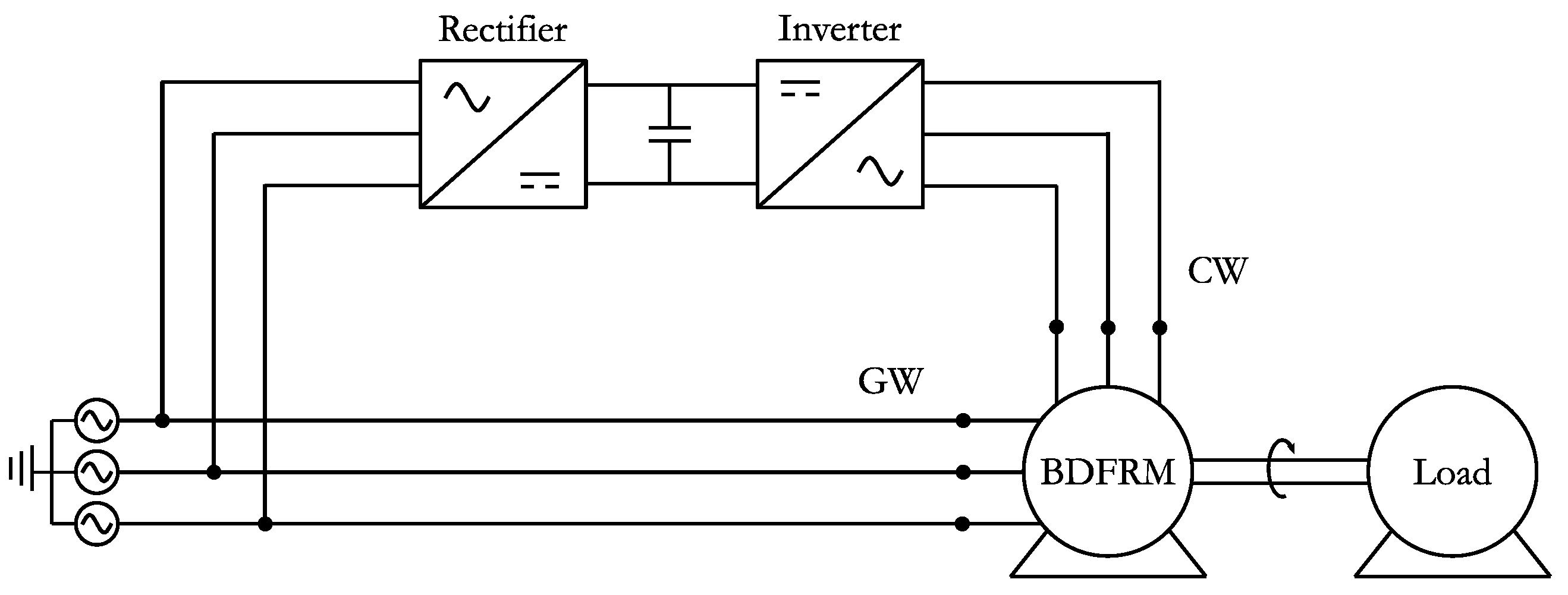
3.1. System Description and Control Requirements

The considered BDFRM system drives a load at variable speed. A system schematic is shown in Figure 1, the mains supply is connected to the grid winding, while the control winding is connected to a variable frequency drive, composed of a rectifier and an inverter coupled with a common DC-bus capacitor. The speed controller of the BDFRM must reach speed setpoints within a 0.5 % error at maximum speed and must be capable of following a ramp with a rate of change of at least 300 rpm/s to a new speed setpoint.

3.2. Cascade Control

Electrical machines are most often controlled by cascade control, containing an inner loop for current control and an outer loop for speed control, as depicted in Figure 2. The inner loop is usually composed of the PI-controllers, designed to compensate for the machine inductances, to ensure fast current and thereby torque control. On the other hand, the outer loop for speed control is typically a P or PI-controller, to meet the desired speed reference. For both synchronous and asynchronous machines, model-based cascade control is the way to go in the industry. This section investigates the feasibility of this rule for the BDFRM.

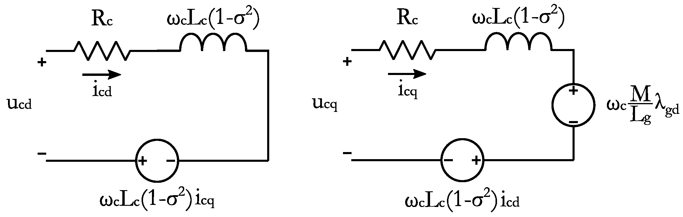
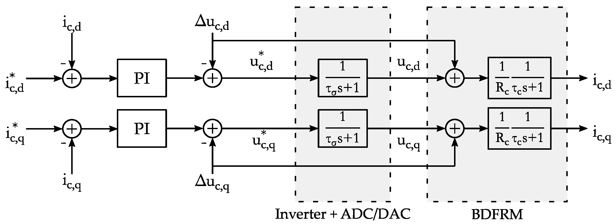
3.2.1. Control Winding Current Control

The only controllable inputs of the BDFRM system are the control winding voltages, via the inverter, while the grid windings are connected to the constant mains supply. Therefore, the grid winding voltages are treated as known disturbances. However, considering Equations (15) and (16), the use of the classic pole-zero cancellation control design method is impeded by the presence of the derivatives of the grid winding currents.

$${\mathrm{u}}_{\mathrm{c},\mathrm{d}}{=\mathrm{R}}_{\mathrm{c}}{\mathrm{i}}_{\mathrm{c},\mathrm{d}}{+\mathrm{L}}_{\mathrm{c}}\frac{{\mathrm{d}(\mathrm{i}}_{\mathrm{c},\mathrm{d}})}{\mathrm{dt}}+\mathrm{M}\frac{\mathrm{d}\left({\mathrm{i}}_{\mathrm{g},\mathrm{d}}\right)}{\mathrm{dt}}{+(\mathsf{\omega }}_{\mathrm{r}}{-\mathsf{\omega }\left)\right(\mathrm{Mi}}_{\mathrm{g},\mathrm{q}}{-\mathrm{L}}_{\mathrm{c}}{\mathrm{i}}_{\mathrm{c},\mathrm{q}})$$

(15)

$${\mathrm{u}}_{\mathrm{c},\mathrm{q}}{=\mathrm{R}}_{\mathrm{c}}{\mathrm{i}}_{\mathrm{c},\mathrm{q}}+{\mathrm{L}}_{\mathrm{c}}\frac{{\mathrm{d}(\mathrm{i}}_{\mathrm{c},\mathrm{d}})}{\mathrm{dt}}-\mathrm{M}\frac{\mathrm{d}\left({\mathrm{i}}_{\mathrm{g},\mathrm{q}}\right)}{\mathrm{dt}}{+(\mathsf{\omega }}_{\mathrm{r}}{-\mathsf{\omega }\left)\right(\mathrm{Mi}}_{\mathrm{g},\mathrm{d}}{+\mathrm{L}}_{\mathrm{c}}{\mathrm{i}}_{\mathrm{c},\mathrm{d}})$$

(16)

The grid winding voltage Equations (6) and (7) allow to eliminate the derivatives of the grid winding currents, which make it then possible to write Equations (17) and (18). By considering ${\mathsf{\Delta }\mathrm{u}}_{\mathrm{c},\mathrm{d}}$, Equation (19), and ${\mathsf{\Delta }\mathrm{u}}_{\mathrm{c},\mathrm{q}}$, Equation (20), as feedforward terms, Equations (17) and (18) will enable the pole-zero cancellation technique to design the PI current controllers.

$${\mathrm{u}}_{\mathrm{c},\mathrm{d}}={\mathrm{R}}_{\mathrm{c}}{\mathrm{i}}_{\mathrm{c},\mathrm{d}}+\frac{\mathrm{d}}{\mathrm{dt}}\left(\left({\mathrm{L}}_{\mathrm{c}}-\frac{{\mathrm{M}}^2}{{\mathrm{L}}_{\mathrm{g}}}\right){\mathrm{i}}_{\mathrm{c},\mathrm{d}}\right)+{\mathsf{\Delta }\mathrm{u}}_{\mathrm{c},\mathrm{d}}$$

(17)

$${\mathrm{u}}_{\mathrm{c},\mathrm{q}}={\mathrm{R}}_{\mathrm{c}}{\mathrm{i}}_{\mathrm{c},\mathrm{q}}\left(\mathrm{t}\right)+\frac{\mathrm{d}}{\mathrm{dt}}\left(\left({\mathrm{L}}_{\mathrm{c}}-\frac{{\mathrm{M}}^2}{{\mathrm{L}}_{\mathrm{g}}}\right){\mathrm{i}}_{\mathrm{c},\mathrm{q}}\right)+{\mathsf{\Delta }\mathrm{u}}_{\mathrm{c},\mathrm{q}}$$

(18)

$${\mathsf{\Delta }\mathrm{u}}_{\mathrm{c},\mathrm{d}}=\frac{\mathrm{M}}{{\mathrm{L}}_{\mathrm{g}}}\left({\mathrm{u}}_{\mathrm{g},\mathrm{d}}{-\mathrm{R}}_{\mathrm{g}}{\mathrm{i}}_{\mathrm{g},\mathrm{d}}-\mathsf{\omega }\left({\mathrm{M}\mathrm{i}}_{\mathrm{c},\mathrm{q}}{-\mathrm{L}}_{\mathrm{g}}{\mathrm{i}}_{\mathrm{g},\mathrm{q}}\right)\right)+\left({\mathsf{\omega }}_{\mathrm{r}}-\mathsf{\omega }\right)\left({\mathrm{M}\mathrm{i}}_{\mathrm{g},\mathrm{q}}{-\mathrm{L}}_{\mathrm{c}}{\mathrm{i}}_{\mathrm{c},\mathrm{q}}\right)$$

(19)

$${\mathsf{\Delta }\mathrm{u}}_{\mathrm{c},\mathrm{q}}=-\frac{\mathrm{M}}{{\mathrm{L}}_{\mathrm{g}}}\left({\mathrm{u}}_{\mathrm{g},\mathrm{q}}{-\mathrm{R}}_{\mathrm{g}}{\mathrm{i}}_{\mathrm{g},\mathrm{q}}\left(\mathrm{t}\right)-\mathsf{\omega }\left({\mathrm{M}\mathrm{i}}_{\mathrm{c},\mathrm{d}}{+\mathrm{L}}_{\mathrm{g}}{\mathrm{i}}_{\mathrm{g},\mathrm{d}}\right)\right)+\left({\mathsf{\omega }}_{\mathrm{r}}-\mathsf{\omega }\right)\left({\mathrm{M}\mathrm{i}}_{\mathrm{g},\mathrm{d}}{+\mathrm{L}}_{\mathrm{c}}{\mathrm{i}}_{\mathrm{c},\mathrm{d}}\right)$$

(20)

The first terms in ${\mathsf{\Delta }\mathrm{u}}_{\mathrm{c},\mathrm{d}}$ and ${\mathsf{\Delta }\mathrm{u}}_{\mathrm{c},\mathrm{q}}$ portray the rate of change of the amplitude of the grid winding flux linkages. These terms, Equations (21) and (22), are therefore negligible with respect to the other terms in ${\mathsf{\Delta }\mathrm{u}}_{\mathrm{c},\mathrm{d}}$ and ${\mathsf{\Delta }\mathrm{u}}_{\mathrm{c},\mathrm{q}}$, particularly when the winding resistances are negligible and the mains supply is stable.

$${\mathrm{u}}_{\mathrm{g},\mathrm{d}}{-\mathrm{R}}_{\mathrm{g}}{\mathrm{i}}_{\mathrm{g},\mathrm{d}}-\mathsf{\omega }\left({\mathrm{M}\mathrm{i}}_{\mathrm{c},\mathrm{q}}{-\mathrm{L}}_{\mathrm{g}}{\mathrm{i}}_{\mathrm{g},\mathrm{q}}\right)={\mathrm{u}}_{\mathrm{g},\mathrm{d}}{-\mathrm{R}}_{\mathrm{g}}{\mathrm{i}}_{\mathrm{g},\mathrm{d}}{+\mathsf{\omega }\mathsf{\lambda }}_{\mathrm{g},\mathrm{q}}\approx 0$$

(21)

$${\mathrm{u}}_{\mathrm{g},\mathrm{q}}{-\mathrm{R}}_{\mathrm{g}}{\mathrm{i}}_{\mathrm{g},\mathrm{q}}-\mathsf{\omega }\left({\mathrm{M}\mathrm{i}}_{\mathrm{c},\mathrm{d}}{+\mathrm{L}}_{\mathrm{g}}{\mathrm{i}}_{\mathrm{g},\mathrm{d}}\right){=\mathrm{u}}_{\mathrm{g},\mathrm{q}}{-\mathrm{R}}_{\mathrm{g}}{\mathrm{i}}_{\mathrm{g},\mathrm{q}}{-\mathsf{\omega }\mathsf{\lambda }}_{\mathrm{g},\mathrm{d}}\approx 0$$

(22)

When inserting Equations (11) and (12), resulting from the FO-frame choice, into Equation (17) to Equation (20) and by introducing the transformer coupling factor $\mathsf{\sigma }=\mathrm{M}/\sqrt{{\mathrm{L}}_{\mathrm{g}}{\mathrm{L}}_{\mathrm{c}}}$, one obtains Equation (23) to Equation (26).

$${\mathrm{u}}_{\mathrm{c},\mathrm{d}}={\mathrm{R}}_{\mathrm{c}}{\mathrm{i}}_{\mathrm{c},\mathrm{d}}+{\mathrm{L}}_{\mathrm{c}} \left({1-\mathsf{\sigma }}^2\right)\frac{{\mathrm{di}}_{\mathrm{c},\mathrm{d}}}{\mathrm{dt}}{+\mathsf{\Delta }\mathrm{u}}_{\mathrm{c},\mathrm{d}}$$

(23)

$${\mathrm{u}}_{\mathrm{c},\mathrm{q}}{=\mathrm{R}}_{\mathrm{c}}{\mathrm{i}}_{\mathrm{c},\mathrm{q}}{+\mathrm{L}}_{\mathrm{c}}\left({1-\mathsf{\sigma }}^2\right)\frac{{\mathrm{di}}_{\mathrm{c},\mathrm{q}}}{\mathrm{dt}}{+\mathsf{\Delta }\mathrm{u}}_{\mathrm{c},\mathrm{q}}$$

(24)

$${\mathsf{\Delta }\mathrm{u}}_{\mathrm{c},\mathrm{d}}=-\left({\mathsf{\omega }}_{\mathrm{r}}-\mathsf{\omega }\right){\mathrm{L}}_{\mathrm{c}}\left({1-\mathsf{\sigma }}^2\right){\mathrm{i}}_{\mathrm{c},\mathrm{q}}$$

(25)

$${\mathsf{\Delta }\mathrm{u}}_{\mathrm{c},\mathrm{q}}=\left({\mathsf{\omega }}_{\mathrm{r}}-\mathsf{\omega }\right)\left(\frac{\mathrm{M}}{{\mathrm{L}}_{\mathrm{g}}}{\mathsf{\lambda }}_{\mathrm{g},\mathrm{d}}{+\mathrm{L}}_{\mathrm{c}}\left({1-\mathsf{\sigma }}^2\right){\mathrm{i}}_{\mathrm{c},\mathrm{d}}\right)$$

(26)

The control winding voltage equations now have the look of the voltage equations of a PMSM with no saliency, except for the presence of ${(\mathsf{\omega }}_{\mathrm{r}}-\mathsf{\omega })$ instead of ${\mathsf{\omega }}_{\mathrm{r}}$ in the induced voltages ${\mathsf{\Delta }\mathrm{u}}_{\mathrm{c},\mathrm{d}}$ and ${\mathsf{\Delta }\mathrm{u}}_{\mathrm{c},\mathrm{q}}$. The equivalent circuit is depicted in Figure 3.

Moreover, disregarding the induced voltages, the current transfer functions are characterized by the same left plane pole, Equation (27).

$${\mathsf{\tau }}_{\mathrm{c}}=\frac{{\mathrm{L}}_{\mathrm{c}}{(1-\mathsf{\sigma }}^2)}{{\mathrm{R}}_{\mathrm{c}}}$$

(27)

To consider the influence of the inverter and delays due to the real-time system it is possible to model them as a first-order system with the time constant ${\mathsf{\tau }}_{\mathsf{\sigma }}$, as proposed by [40]:

$${\mathsf{\tau }}_{\mathsf{\sigma }}{=\mathrm{T}}_{\mathrm{s}}{+\mathrm{T}}_{\mathrm{PWM}}{+\mathsf{\tau }}_{\mathrm{filt}}$$

(28)

The time constant ${\mathsf{\tau }}_{\mathsf{\sigma }}$ is composed of the sampling time of the real-time target ${\mathrm{T}}_{\mathrm{s}}$, the switching period ${\mathrm{T}}_{\mathrm{PWM}}$, which is the time needed to convert the reference voltage signal to a real voltage at the machine terminals, and the measurement filter time constant ${\mathsf{\tau }}_{\mathrm{filt}}$.

The requirements are set to design two identical PI-controllers for the currents ${\mathrm{i}}_{\mathrm{c},\mathrm{d}}$ and ${\mathrm{i}}_{\mathrm{c},\mathrm{q}}$ with feed forward voltage compensation, so that the dominant pole produced by the modified control winding inductance ${\mathrm{L}}_{\mathrm{c}}\left({1-\mathsf{\sigma }}^2\right)$ is compensated for. The complete system is schematically depicted in Figure 4.

To obtain optimal damping ($\mathsf{\zeta }=\frac{1}{\sqrt{2}}$) of the closed-loop current response, the PI-controller parameters must be Equations (29) and (30).

$${\mathsf{\tau }}_{\mathrm{i}}{=\mathsf{\tau }}_{\mathrm{c}}$$

(29)

$${\mathrm{K}}_{\mathrm{i}}=\frac{{\mathrm{R}}_{\mathrm{c}}{\mathsf{\tau }}_{\mathrm{i}}}{{2\mathsf{\tau }}_{\mathsf{\sigma }}}$$

(30)

This tuning method is well-documented and applied in conventional machines, as detailed in [40,41]. Following [40], The second order system can be simplified as a first order system, Equation (31), with an equivalent time constant ${\mathsf{\tau }}_{\mathrm{eq}}$, Equation (32), and a phase margin of 65°:

$${\mathrm{G}}_{\mathrm{CL}}=\frac{1}{{2\mathsf{\tau }}_{\mathsf{\sigma }}^2{\mathrm{s}}^2{+2\mathsf{\tau }}_{\mathsf{\sigma }}\mathrm{s}+1}\approx \frac{1}{{\mathsf{\tau }}_{\mathrm{eq}}\mathrm{s}+1}$$

(31)

$${\mathsf{\tau }}_{\mathrm{eq}}=\sqrt{2}{2\mathsf{\tau }}_{\mathsf{\sigma }}$$

(32)

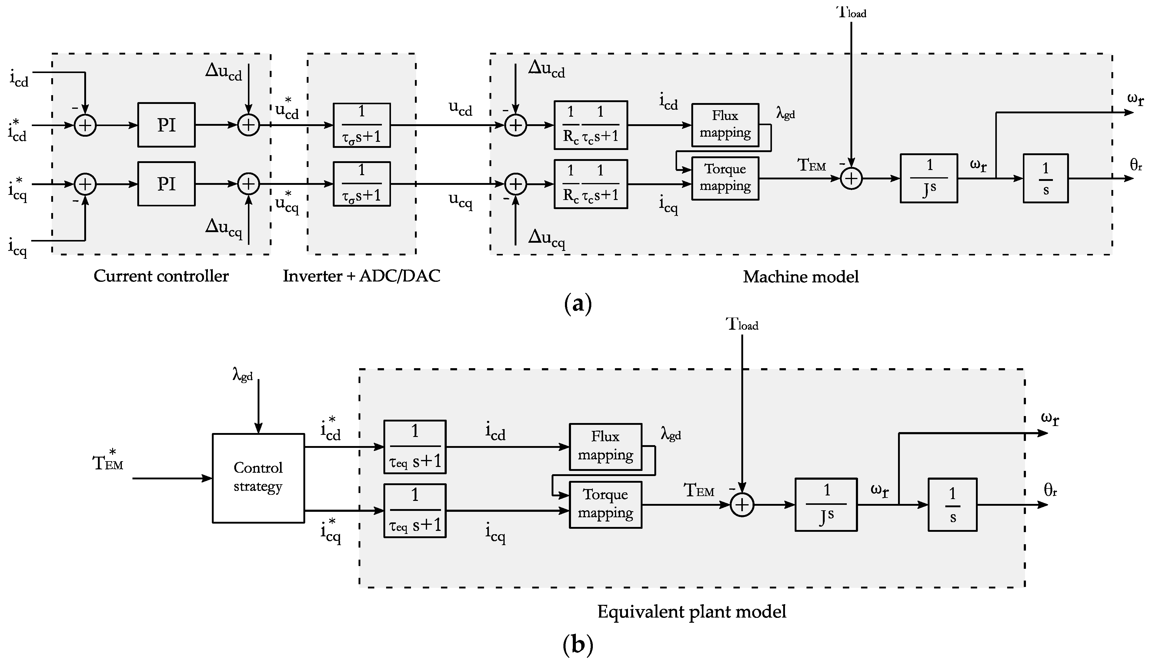
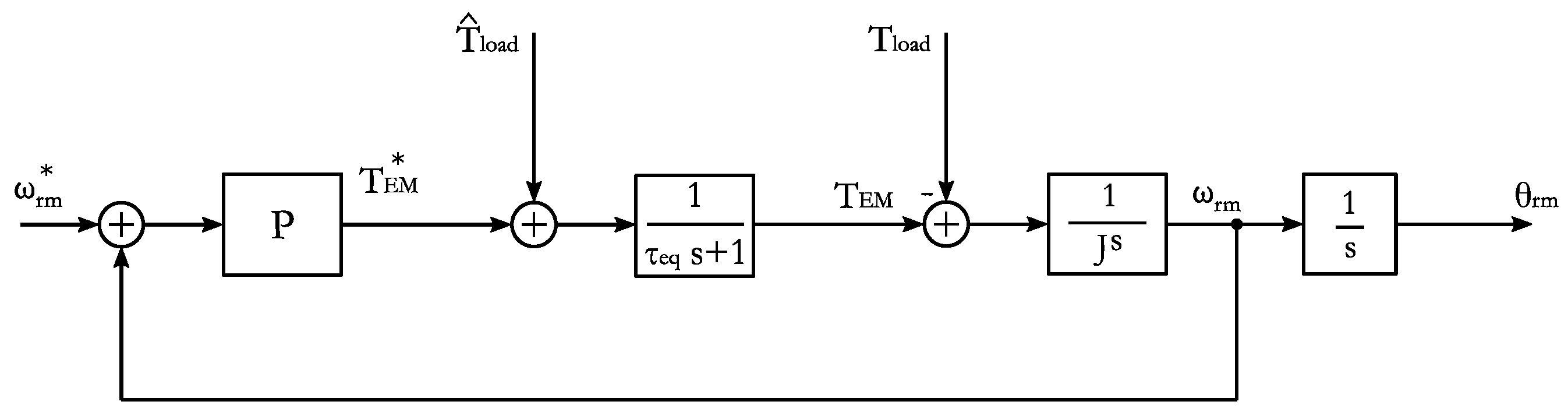
3.2.2. Speed Control

The inner control winding current control loop, shown in Figure 5a, and the torque Equation (5) allow to operate the BDFRM in torque control by providing a torque/current mapping for ${\mathrm{i}}_{\mathrm{c},\mathrm{q}}$. On the other hand, ${\mathrm{i}}_{\mathrm{c},\mathrm{d}}$ can be selected to achieve other control requirements such as reactive power flow or maximum torque per inverter ampere (MPTIA). The closed loop control winding current control can be simplified with Equations (31) and (32), providing an equivalent plant model as in Figure 5b. The transfer function in Equation (31) is also employed as an approximation for the open-loop response of the electromagnetic torque reference ${\mathrm{T}}_{\mathrm{EM}}^{*}$, which facilitates the control system design for the speed.

In [40], a speed controller with a simple P-controller in combination with a load torque compensation was proposed for the PMSMs. Based on mechanical Equation (6) and the approximation of the open loop response of the electromagnetic torque reference, Equation (31), one obtains a system as in Figure 6, with the open loop transfer function as in Equation (33) for the speed reference ${\mathsf{\omega }}_{\mathrm{rm}}^{*}$.

$${\mathrm{G}}_{\mathrm{OL}}={\mathrm{K}}_{\mathrm{n}}\frac{1}{\mathrm{Js}}\frac{1}{{\mathsf{\tau }}_{\mathrm{eq}}\mathrm{s}+1}$$

(33)

To obtain optimal damping ($\mathsf{\zeta }=\frac{1}{\sqrt{2}}$) of the closed-loop speed response, the P-controller gain becomes Equation (34):

$${\mathrm{K}}_{\mathrm{n}}=\frac{\mathrm{J}}{{2\mathsf{\tau }}_{\mathrm{eq}}}$$

(34)

The reader is referred to [40,41] for further details on the tuning method. A PI-controller could also be used, at the expense of a more complicated tuning method for the controller. Well established tuning methods for this kind of problem such as the symmetric optimum or Kessler’s method can then be used [40,41,42].

Notwithstanding the acquired simplicity of the speed controller with a simple gain ${\mathrm{K}}_{\mathrm{n}}$, the disadvantage is that a load compensation and thus a load torque estimate is required, which includes the mechanical and iron losses. This necessitates the use of an observer, which will be discussed in detail in Section 4.

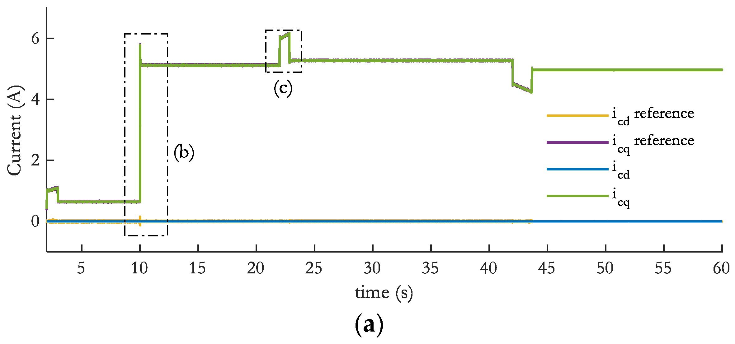
3.2.3. Simulation Results

As a first step to verify that the control design meets the requirements, a Simulink BDFRM model is constructed, and a simulation is performed. The BDFRM electrical equations are modelled in a VO frame in the state space representation, Equation (35), with matrix the ${\mathbf{A}}_{\mathsf{\lambda }}$ as in Equation (36). The mechanical equations employed for the speed and torque are Equations (37) and (10), respectively. The speed equation considers viscous friction with the viscous friction coefficient B:

$$\frac{\mathrm{d}}{\mathrm{dt}}\left[\begin{array}{c}{\mathsf{\lambda }}_{\mathrm{g},\mathrm{d}}\\ {\mathsf{\lambda }}_{\mathrm{g},\mathrm{q}}\\ {\mathsf{\lambda }}_{\mathrm{c},\mathrm{d}}\\ {\mathsf{\lambda }}_{\mathrm{c},\mathrm{q}}\end{array}\right]={\mathbf{A}}_{\mathsf{\lambda }}\left[\begin{array}{c}{\mathsf{\lambda }}_{\mathrm{g},\mathrm{d}}\\ {\mathsf{\lambda }}_{\mathrm{g},\mathrm{q}}\\ {\mathsf{\lambda }}_{\mathrm{c},\mathrm{d}}\\ {\mathsf{\lambda }}_{\mathrm{c},\mathrm{q}}\end{array}\right]+\left[\begin{array}{c}{\mathrm{u}}_{\mathrm{g},\mathrm{d}}\\ {\mathrm{u}}_{\mathrm{g},\mathrm{q}}\\ {\mathrm{u}}_{\mathrm{c},\mathrm{d}}\\ {\mathrm{u}}_{\mathrm{c},\mathrm{q}}\end{array}\right]$$

(35)

$${\mathbf{A}}_{\mathsf{\lambda }}=\left[\begin{array}{cccc}\frac{{\mathrm{L}}_{\mathrm{c}}{\mathrm{R}}_{\mathrm{g}}}{\left({\mathrm{M}}^2-{\mathrm{L}}_{\mathrm{c}}{\mathrm{L}}_{\mathrm{g}}\right)}& \mathsf{\omega }& -\frac{{\mathrm{MR}}_{\mathrm{g}}}{\left({\mathrm{M}}^2-{\mathrm{L}}_{\mathrm{c}}{\mathrm{L}}_{\mathrm{g}}\right)}& 0\\ -\mathsf{\omega }& \frac{{\mathrm{L}}_{\mathrm{c}}{\mathrm{R}}_{\mathrm{g}}}{\left({\mathrm{M}}^2-{\mathrm{L}}_{\mathrm{c}}{\mathrm{L}}_{\mathrm{g}}\right)}& 0& \frac{{\mathrm{MR}}_{\mathrm{g}}}{\left({\mathrm{M}}^2-{\mathrm{L}}_{\mathrm{c}}{\mathrm{L}}_{\mathrm{g}}\right)}\\ -\frac{{\mathrm{MR}}_{\mathrm{c}}}{\left({\mathrm{M}}^2-{\mathrm{L}}_{\mathrm{c}}{\mathrm{L}}_{\mathrm{g}}\right)} & 0& \frac{{\mathrm{L}}_{\mathrm{g}}{\mathrm{R}}_{\mathrm{c}}}{\left({\mathrm{M}}^2-{\mathrm{L}}_{\mathrm{c}}{\mathrm{L}}_{\mathrm{g}}\right)}& \left({\mathsf{\omega }}_{\mathrm{r}}-\mathsf{\omega }\right)\\ 0& \frac{{\mathrm{MR}}_{\mathrm{c}}}{\left({\mathrm{M}}^2-{\mathrm{L}}_{\mathrm{c}}{\mathrm{L}}_{\mathrm{g}}\right)}& -\left({\mathsf{\omega }}_{\mathrm{r}}-\mathsf{\omega }\right)& \frac{{\mathrm{L}}_{\mathrm{g}}{\mathrm{R}}_{\mathrm{c}}}{\left({\mathrm{M}}^2-{\mathrm{L}}_{\mathrm{c}}{\mathrm{L}}_{\mathrm{g}}\right)}\end{array}\right]$$

(36)

$$\mathrm{J}\frac{{\mathrm{d}\mathsf{\Omega }}_{\mathrm{r}}}{\mathrm{dt}}{=\mathrm{T}}_{\mathrm{EM}}{-\mathrm{T}}_{\mathrm{load}}{-\mathrm{B}\mathsf{\Omega }}_{\mathrm{r}}$$

(37)

The mains supply is modelled as an ideal three-phase voltage source and supplies the grid winding while the control winding is fed by the inverter, modelled as an ideal voltage source inverter (VSI), using Sine Wave Pulse Width Modulation (SPWM).

The BDFRM under consideration is a 750 W machine at 750 rpm, the parameters are given in

Table 1. Parameters used for the BDFRM simulations.

Parameter	Value	Parameter	Value
pr/pg/pc	6/2/4	Ig (Arms)	5.0
Lg (mH)	73.2	Ic (Arms)	2.5
Lc (mH)	156.3	T (Nm)	9.5
M (mH)	62.6	J (kg m2)	0.034
Rg ($\mathsf{\Omega }$)	10.0	B (Nm s/rad)	0.008
Rc ($\mathsf{\Omega }$)	15.0	${\mathsf{\tau }}_{\mathrm{i}}$	145.8
Ugn (Vrms)	120	Kn,current	171.4
Udc (Vdc)	540	Kn,speed	13.4
fswitch (kHz)	5

.

The simulation shows in Figure 7a the successful control of the speed over a speed range of 500–1000 RPM and a ramp-up/down of 300 RPM/s. Start-up of the machine happens in induction mode, i.e., with the control windings short-circuited, and at no-load, as shown in Figure 7b. The machine is loaded with a step from 40% to 100% of the rated torque after 10 s of simulation.

The response of the control winding current controllers during the simulation is depicted in Figure 8a and shows satisfying performances, especially during transient behavior, at the load step from 40% to 100%, as in Figure 8b, and during speed up/down, as depicted in Figure 8c.

In this simulation, ideal signals are used for the load torque, shaft speed and the grid winding flux linkage. The goal is to demonstrate the validity of the assumptions in Equations (21) and (22), allowing the simplification of the model used for the control design. The simulation shows good performance of the implemented cascade control, confirming the validity of the assumptions that were made.

To bridge the gap towards the control of a real BDFRM, the load torque, shaft speed and FO frame angle need to be estimated, which is the topic of Section 4.

4. Kalman Filtering

The Kalman Filter (KF) is an optimal recursive data processing algorithm for linear time invariant (LTI) systems [43]. It is called optimal because, while assuming the state estimates and measurements are Gaussian Random Variables (GRV), it yields an estimation with the smallest error covariance matrix, making it a minimum mean-square error estimator [44]. Additionally, it benefits of all the available measurements, regardless of their precision. It is called recursive because the Kalman filter produces the estimates without reprocessing all available data at each iteration. It is widely used for estimation and tracking problems thanks to its simplicity, optimality, and robustness [45]. The algorithm consists of a prediction step, based on knowledge of the system, and estimates of the previous completed step, and an update step, which utilizes the measurements to update the prediction. The KF, however, only supports LTIs and therefore requires more sophisticated Kalman Filters to be valuable for nonlinear systems.

The KF for nonlinear systems seems to be, above all, the extended Kalman filter (EKF), used for a multitude of applications, including electric motors [46,47,48,49]. The EKF is based on the same algorithm as its linear counterpart but employs a first order linearization of the general state-transition- and observation function to obtain the mean state estimate and covariance matrix. However, if this local linearity assumption is violated, the EKF can have serious instability problems. Moreover, the required analytical Jacobian derivations are heavy, prone to human errors and arduous to modify [45], especially during rapid control prototyping. Consequently, an unscented Kalman filter (UKF) is considered as our observer. One of the main drives to use a Kalman filter in this paper is its ability to yield one state estimate by merging different system measurements.

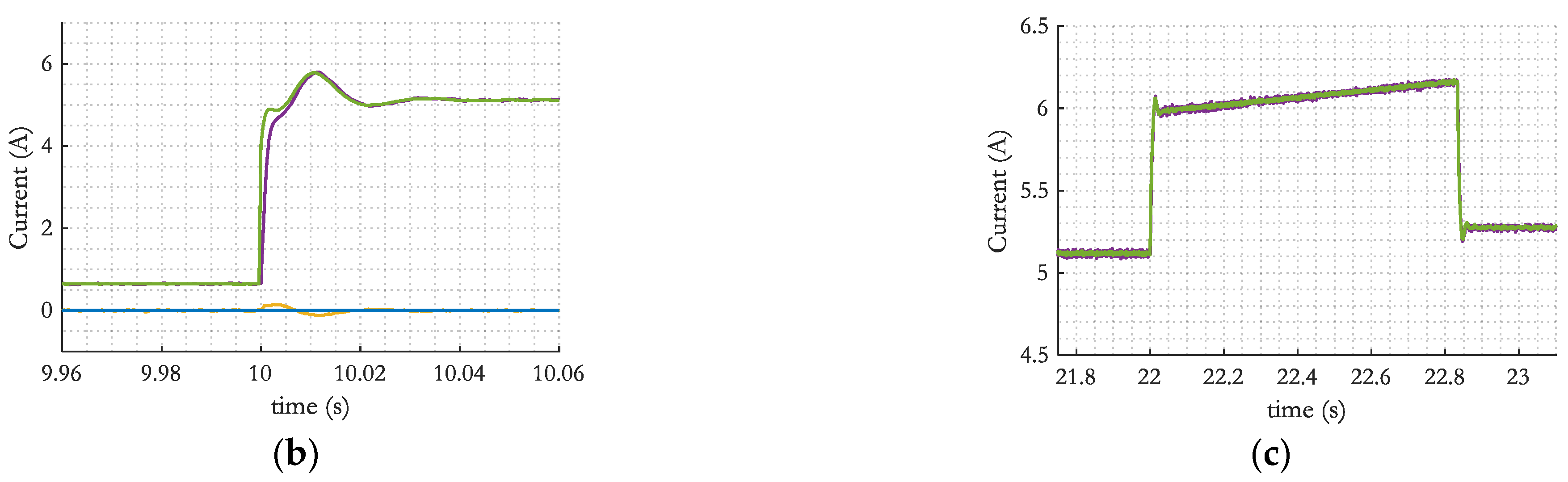
4.1. The Unscented Kalman Filter

The UKF takes advantage of the Unscented Transformation (UT) and is introduced by Julier and Uhlmann in [45]. Whereas the EKF propagates the GRV analytically through a first order linearization of the nonlinear system, hence resulting in a ‘first order’ approximation of the optimal estimations, the UKF carefully selects a minimal set of sample points, called the sigma points, that capture the true mean and covariance of the GRV and propagates these sigma points through the system nonlinear dynamics, thereby achieving an estimation of the posterior mean and covariance accurately up to the third order [50]. The UKF overcomes the EKF approximation flaws and, consequently, results in a better accuracy level and a better performance for a variety of applications overall [50,51,52,53,54], while keeping the actual implementation more adaptable than the EKF as only the state transition and observation functions need to be altered when changing the system model. The difference between the EKF and UKF is illustrated in Figure 9. In Figure 9b, one can see the mean is biased and the propagation through the linearized system is inconsistent since the actual covariance ellipse is not covered by the EKF estimation [45].

The UKF considers a state transition function, Equation (38), and a measurement function, Equation (39), in function of the state $\mathbf{x}$, input $\mathbf{u}$ and process and measurement noises w and v, respectively.

$${\mathbf{x}}_{\mathrm{k}+1}=\mathrm{g}\left({\mathbf{x}}_{\mathrm{k}},{\mathbf{u}}_{\mathrm{k}}\right)+{\mathbf{w}}_{\mathrm{k}}$$

(38)

$${\mathbf{y}}_{\mathrm{k}}=\mathrm{h}({\mathbf{x}}_{\mathrm{k}},{\mathbf{u}}_{\mathrm{k}})+{\mathbf{v}}_{\mathrm{k}}$$

(39)

The KF assumes the noises to be Gaussian with zero mean and uncorrelated over time (white), thus ${\mathbf{w}}_{\mathrm{k}}\sim \mathrm{N}(0,\mathbf{Q})$ and ${\mathbf{v}}_{\mathrm{k}}\sim \mathrm{N}(0,\mathbf{R})$, where Q and R are the covariance matrices. These covariance matrices Q and R are supposed to be known and this is the main difficulty for implementing a KF. The latter can be estimated based on measurements, while the former is more difficult to determine as it contains noise introduced by the system itself together with model inaccuracies. Although some tuning methods exist [55,56,57], the tuning of Q and R adds an important layer of complexity. The good performance of a Kalman filter strongly depends on the correct setting of these matrices.

The UKF algorithm, as described in [54], starts with an initial state estimate ${\mathbf{x}}_{0|0}$ and its covariance matrix ${\mathbf{P}}_{0|0}$. For an arbitrary vector ${\mathbf{X}}_{\mathrm{n}|\mathrm{m}}$, its subscripts mean: the vector X at time instant n, determined with knowledge up to and including time instant m. The first steps of the UKF algorithm, at time step k − 1, are Equation (40) to Equation (43). In Equation (40), the set of (2n + 1) sigma points ${\mathsf{\chi }}_{\mathrm{i}}$ is generated, with n being the dimension of the state vector x, while the subscript j of ${\left(\sqrt{{\mathbf{P}}_{\mathrm{k}-1|\mathrm{k}-1}}\right)}_{\mathrm{j}}$ represent the ${\mathrm{j}}^{\mathrm{th}}$ column of the matrix. In Equation (41) to Equation (43), $\mathsf{\eta }$ and the weights ${\mathrm{w}}_{\mathrm{i}}$, corresponding to their respective sigma points, are generated, with $\mathsf{\kappa }$ a degree of freedom to tune the UKF to diminish prediction errors. The weights are used to average the sigma points and can take different shapes in the literature; therefore the weights are chosen in their most simple form according to [45,58]. As shown by Equations (44) and (45), the sigma points capture the true mean and covariance of the state estimate [58].

Generation of 2n + 1 sigma points:

$${\left[{\mathsf{\chi }}_0,{\mathsf{\chi }}_1,\dots ,{\mathsf{\chi }}_{\mathrm{n}+1},\dots ,{\mathsf{\chi }}_{2\mathrm{n}}\right]}_{\mathrm{k}-1|\mathrm{k}-1}=\left[{\hat{\mathbf{x}}}_{\mathrm{k}-1|\mathrm{k}-1},\left({\hat{\mathbf{x}}}_{\mathrm{k}-1|\mathrm{k}-1}+\mathsf{\eta }{\left(\sqrt{{\mathbf{P}}_{\mathrm{k}-1|\mathrm{k}-1}}\right)}_1\right),\dots ,\left({\hat{\mathbf{x}}}_{\mathrm{k}-1|\mathrm{k}-1}-\mathsf{\eta }{\left(\sqrt{{\mathbf{P}}_{\mathrm{k}-1|\mathrm{k}-1}}\right)}_{\mathrm{n}+1}\right),\dots \right]$$

(40)

$$\mathsf{\eta }=\sqrt{\mathrm{n}+\mathsf{\kappa }}$$

(41)

$${\mathrm{w}}_0=\frac{\mathsf{\kappa }}{\mathrm{n}+\mathsf{\kappa }}$$

(42)

$${\mathrm{w}}_{\mathrm{i}}=\frac{1}{2\left(\mathrm{n}+\mathsf{\kappa }\right)}$$

(43)

$$\overline{\mathbf{x}}=\mathrm{E}\left[\mathbf{x}\right]\approx {\displaystyle \sum _{\mathrm{i}=0}^{2\mathrm{n}}{\mathrm{w}}_{\mathrm{i}}}{\mathsf{\chi }}_{\mathrm{i}}=\hat{\mathbf{x}}$$

(44)

$$\mathrm{E}\left[(\mathbf{x}-\overline{\mathbf{x}}){(\mathbf{x}-\overline{\mathbf{x}})}^{\mathrm{T}}\right]\approx {\displaystyle \sum _{\mathrm{i}=0}^{2\mathrm{n}}{\mathrm{w}}_{\mathrm{i}}}[{\mathsf{\chi }}_{\mathrm{i},\mathrm{k}|\mathrm{k}-1}-{\hat{\mathbf{x}}}_{\mathrm{k}|\mathrm{k}-1}]{[{\mathsf{\chi }}_{\mathrm{i},\mathrm{k}|\mathrm{k}-1}-{\hat{\mathbf{x}}}_{\mathrm{k}|\mathrm{k}-1}]}^{\mathrm{T}}$$

(45)

Next, the prediction step is performed, where the weighted mean of the predicted sigma points ${\mathsf{\chi }}_{\mathrm{i},\mathrm{k}|\mathrm{k}-1}$, obtained with Equation (46), yield with Equation (47) the predicted state ${\hat{\mathbf{x}}}_{\mathrm{k}|\mathrm{k}-1}$. The predicted covariance matrix ${\mathbf{P}}_{\mathrm{k}|\mathrm{k}-1}$ is obtained with Equation (48). Thereafter, a measurement prediction ${\hat{\mathbf{y}}}_{\mathrm{k}|\mathrm{k}-1}$ is obtained with Equations (49) and (50).

Prediction by mapping sigma points:

$${\mathsf{\chi }}_{\mathrm{i},\mathrm{k}|\mathrm{k}-1}=\mathrm{g}\left({\mathsf{\chi }}_{\mathrm{i},\mathrm{k}-1|\mathrm{k}-1},{\mathbf{u}}_{\mathrm{k}}\right)$$

(46)

$${\hat{\mathbf{x}}}_{\mathrm{k}|\mathrm{k}-1}={\displaystyle \sum _{\mathrm{i}=0}^{2\mathrm{n}}{\mathrm{w}}_{\mathrm{i}}}{\mathsf{\chi }}_{\mathrm{i},\mathrm{k}|\mathrm{k}-1}$$

(47)

$${\mathbf{P}}_{\mathrm{k}|\mathrm{k}-1}={\displaystyle \sum _{\mathrm{i}=0}^{2\mathrm{n}}{\mathrm{w}}_{\mathrm{i}}}[{\mathsf{\chi }}_{\mathrm{i},\mathrm{k}|\mathrm{k}-1}-{\hat{\mathbf{x}}}_{\mathrm{k}|\mathrm{k}-1}]{[{\mathsf{\chi }}_{\mathrm{i},\mathrm{k}|\mathrm{k}-1}-{\hat{\mathbf{x}}}_{\mathrm{k}|\mathrm{k}-1}]}^{\mathrm{T}}+\mathbf{Q}$$

(48)

$${\mathbf{Y}}_{\mathrm{i},\mathrm{k}|\mathrm{k}-1}=\mathbf{h}\left({\mathsf{\chi }}_{\mathrm{i},\mathrm{k}-1|\mathrm{k}-1},{\mathbf{u}}_{\mathrm{k}}\right)$$

(49)

$${\hat{\mathbf{y}}}_{\mathrm{k}|\mathrm{k}-1}={\displaystyle \sum _{\mathrm{i}=0}^{2\mathrm{n}}{\mathrm{w}}_{\mathrm{i}}}{\mathbf{Y}}_{\mathrm{i},\mathrm{k}|\mathrm{k}-1}$$

(50)

The latest step is the measurement update, where the measurement information is used to obtain a better state estimate. The error $\Delta {\mathbf{y}}_{\mathrm{k}}$ between the actual and estimated measurement is determined with Equation (51). Next, the covariance matrices ${\mathbf{S}}_{\mathrm{k}}$, Equation (52), influenced by the tuneable covariance measurement noise matrix R, and ${\mathbf{S}}_{\mathrm{k}}^{\mathrm{xy}}$ Equation (53) result in the Kalman gain K Equation (54), which is the weighting matrix used to update the state estimate and the process covariance such that one obtains ${\hat{\mathbf{x}}}_{\mathrm{k}|\mathrm{k}}$, Equation (55), and ${\mathbf{P}}_{\mathrm{k}|\mathrm{k}}$, Equation (56). When more confidence is put into the measurements, R and ${\mathbf{S}}_{\mathrm{k}}$ will decrease, consequently ${\mathbf{K}}_{\mathrm{k}}$ will increase and eventually more weight is given to the measurement (with respect to the model) to update the state estimate.

Measurement update:

$$\mathsf{\Delta }{\mathbf{y}}_{\mathrm{k}}={\mathbf{y}}_{\mathrm{k}}-{\hat{\mathbf{y}}}_{\mathrm{k}|\mathrm{k}-1}$$

(51)

$${\mathbf{S}}_{\mathrm{k}}={\displaystyle \sum _{\mathrm{i}=0}^{2\mathrm{n}}{\mathrm{w}}_{\mathrm{i}}^{\left(\mathrm{c}\right)}}[{\mathbf{Y}}_{\mathrm{i},\mathrm{k}|\mathrm{k}-1}-{\hat{\mathbf{y}}}_{\mathrm{k}|\mathrm{k}-1}]{[{\mathbf{Y}}_{\mathrm{i},\mathrm{k}|\mathrm{k}-1}-{\hat{\mathbf{y}}}_{\mathrm{k}|\mathrm{k}-1}]}^{\mathrm{T}}+\mathbf{R}$$

(52)

$${\mathbf{S}}_{\mathrm{k}}^{\mathrm{xy}}={\displaystyle \sum _{\mathrm{i}=0}^{2\mathrm{n}}{\mathrm{w}}_{\mathrm{i}}^{\left(\mathrm{c}\right)}[{\mathsf{\chi }}_{\mathrm{i},\mathrm{k}|\mathrm{k}-1}-{\hat{\mathbf{x}}}_{\mathrm{k}|\mathrm{k}-1}]{[{\mathbf{Y}}_{\mathrm{i},\mathrm{k}|\mathrm{k}-1}-{\hat{\mathbf{y}}}_{\mathrm{k}|\mathrm{k}-1}]}^{\mathrm{T}}}$$

(53)

$${\mathbf{K}}_{\mathrm{k}}={\mathbf{S}}_{\mathrm{k}}^{\mathrm{xy}}{\mathbf{S}}_{\mathrm{k}}^{-1}$$

(54)

$${\hat{\mathbf{x}}}_{\mathrm{k}|\mathrm{k}}={\hat{\mathbf{x}}}_{\mathrm{k}|\mathrm{k}-1}+{\mathbf{K}}_{\mathrm{k}}\Delta {\mathbf{y}}_{\mathrm{k}}$$

(55)

$${\mathbf{P}}_{\mathrm{k}|\mathrm{k}}={\mathbf{P}}_{\mathrm{k}|\mathrm{k}-1}-{\mathbf{K}}_{\mathrm{k}}{\mathbf{S}}_{\mathrm{k}}{\mathbf{K}}_{\mathrm{k}}^{\mathrm{T}}$$

(56)

4.2. Model Description

The UKF relies on a model of the BDFRM to predict the state. The state vector of this model contains for the electrical states the flux linkages in the dq-reference frame and for the mechanical states the electrical rotor speed and position and the load torque. The rate of change of the load torque is considered zero, as the load torque is assumed to vary slowly relative to the UKF sampling time. The state transition function $\mathrm{g}\left(\mathbf{x},\mathbf{u}\right)$ then becomes Equation (57):

$$\dot{\mathbf{x}}=\frac{\mathrm{d}}{\mathrm{dt}}\left[\begin{array}{c}{\mathsf{\lambda }}_{\mathrm{g},\mathrm{d}}\\ {\mathsf{\lambda }}_{\mathrm{g},\mathrm{q}}\\ {\mathsf{\lambda }}_{\mathrm{cd}}\\ {\mathsf{\lambda }}_{\mathrm{c},\mathrm{q}}\\ {\mathsf{\omega }}_{\mathrm{r}}\\ {\mathsf{\theta }}_{\mathrm{r}}\\ {\mathrm{T}}_{\mathrm{load}}\end{array}\right]=\mathbf{g}\left(\mathbf{x},\mathbf{u}\right)=\left[\begin{array}{c}{\mathbf{A}}_{\mathsf{\lambda }}\left[\begin{array}{c}{\mathsf{\lambda }}_{\mathrm{g},\mathrm{d}}\\ {\mathsf{\lambda }}_{\mathrm{g},\mathrm{q}}\\ {\mathsf{\lambda }}_{\mathrm{c},\mathrm{d}}\\ {\mathsf{\lambda }}_{\mathrm{c},\mathrm{q}}\end{array}\right]+\mathbf{T}\left[\begin{array}{c}{\mathrm{u}}_{\mathrm{g},\mathsf{\alpha }}\\ {\mathrm{u}}_{\mathrm{g},\mathsf{\beta }}\\ {\mathrm{u}}_{\mathrm{c},\mathsf{\alpha }}\\ {\mathrm{u}}_{\mathrm{c},\mathsf{\beta }}\end{array}\right]\\ 0\\ 0\\ 0\end{array}\right]+\left[\begin{array}{c}0\\ 0\\ 0\\ 0\\ \frac{{\mathrm{p}}_{\mathrm{r}}^2{\mathrm{M}\mathsf{\lambda }}_{\mathrm{g},\mathrm{d}}{\mathsf{\lambda }}_{\mathrm{c},\mathrm{q}}}{\mathrm{J}\left({\mathrm{M}}^2-{\mathrm{L}}_{\mathrm{g}}{\mathrm{L}}_{\mathrm{c}}\right)}-\frac{{\mathrm{p}}_{\mathrm{r}}}{\mathrm{J}}{\mathrm{T}}_{\mathrm{load}}\\ {\mathsf{\omega }}_{\mathrm{r}}\\ 0\end{array}\right]$$

(57)

$${\mathbf{A}}_{\mathsf{\lambda }}=\left[\begin{array}{cccc}\frac{{\mathrm{L}}_{\mathrm{c}}{\mathrm{R}}_{\mathrm{g}}}{\left({\mathrm{M}}^2-{\mathrm{L}}_{\mathrm{c}}{\mathrm{L}}_{\mathrm{g}}\right)}& \mathsf{\omega }& -\frac{{\mathrm{MR}}_{\mathrm{g}}}{\left({\mathrm{M}}^2-{\mathrm{L}}_{\mathrm{c}}{\mathrm{L}}_{\mathrm{g}}\right)}& 0\\ -\mathsf{\omega }& \frac{{\mathrm{L}}_{\mathrm{c}}{\mathrm{R}}_{\mathrm{g}}}{\left({\mathrm{M}}^2-{\mathrm{L}}_{\mathrm{c}}{\mathrm{L}}_{\mathrm{g}}\right)}& 0& \frac{{\mathrm{MR}}_{\mathrm{g}}}{\left({\mathrm{M}}^2-{\mathrm{L}}_{\mathrm{c}}{\mathrm{L}}_{\mathrm{g}}\right)}\\ -\frac{{\mathrm{MR}}_{\mathrm{c}}}{\left({\mathrm{M}}^2-{\mathrm{L}}_{\mathrm{c}}{\mathrm{L}}_{\mathrm{g}}\right)} & 0& \frac{{\mathrm{L}}_{\mathrm{g}}{\mathrm{R}}_{\mathrm{c}}}{\left({\mathrm{M}}^2-{\mathrm{L}}_{\mathrm{c}}{\mathrm{L}}_{\mathrm{g}}\right)}& \left({\mathsf{\omega }}_{\mathrm{r}}-\mathsf{\omega }\right)\\ 0& \frac{{\mathrm{MR}}_{\mathrm{c}}}{\left({\mathrm{M}}^2-{\mathrm{L}}_{\mathrm{c}}{\mathrm{L}}_{\mathrm{g}}\right)}& -\left({\mathsf{\omega }}_{\mathrm{r}}-\mathsf{\omega }\right)& \frac{{\mathrm{L}}_{\mathrm{g}}{\mathrm{R}}_{\mathrm{c}}}{\left({\mathrm{M}}^2-{\mathrm{L}}_{\mathrm{c}}{\mathrm{L}}_{\mathrm{g}}\right)}\end{array}\right]$$

(58)

$$\mathbf{T}=\left[\begin{array}{cccc}\cos \mathsf{\theta }& -\sin \mathsf{\theta }& 0& 0\\ \sin \mathsf{\theta }& \cos \mathsf{\theta }& 0& 0\\ 0& 0& \cos ({\mathsf{\theta }}_{\mathrm{r}}-\mathsf{\theta })& -\sin ({\mathsf{\theta }}_{\mathrm{r}}-\mathsf{\theta })\\ 0& 0& \sin ({\mathsf{\theta }}_{\mathrm{r}}-\mathsf{\theta })& \cos ({\mathsf{\theta }}_{\mathrm{r}}-\mathsf{\theta })\end{array}\right]$$

(59)

The measurements available for the UKF are the phase currents of both the grid and current windings in the stationary $\mathsf{\alpha }\mathsf{\beta }$-frame, the mechanical speed measured with an encoder and an estimate of the rotor angle. The rotor angle estimate, Equation (60), is extensively reported in the literature [20,27,59], and is used here to help the UKF find the FO frame and to filter the encoder speed signal. The measurements and the rotor angle estimate yield Equation (61) for the observation function $\mathrm{h}(\mathbf{x},\mathbf{u})$.

$${\hat{\mathsf{\theta }}}_{\mathrm{r}}={\mathsf{\theta }}_{\mathrm{g}}+\mathrm{a}\tan \left(\frac{{\mathrm{i}}_{\mathrm{c},\mathsf{\beta }}}{{\mathrm{i}}_{\mathrm{c},\mathsf{\alpha }}}\right)-\mathrm{a}\tan \left(\frac{{\hat{\text{ı}}}_{c,q}}{{\hat{\text{ı}}}_{c,d}}\right)$$

(60)

$$\mathbf{y}=\left[\begin{array}{c}{\mathrm{i}}_{\mathrm{g},\mathsf{\alpha }}\\ {\mathrm{i}}_{\mathrm{g},\mathsf{\beta }}\\ {\mathrm{i}}_{\mathrm{c},\mathsf{\alpha }}\\ {\mathrm{i}}_{\mathrm{c},\mathsf{\beta }}\\ {\Omega }_{\mathrm{r}}\\ {\hat{\mathsf{\theta }}}_{\mathrm{r}}\end{array}\right]=\mathrm{h}\left(\mathbf{x},\mathbf{u}\right)=\left[\begin{array}{c}{\mathbf{C}}_{4\mathrm{x}4}\left[\begin{array}{c}{\mathsf{\lambda }}_{\mathrm{g},\mathrm{d}}\\ {\mathsf{\lambda }}_{\mathrm{g},\mathrm{q}}\\ {\mathsf{\lambda }}_{\mathrm{c},\mathrm{d}}\\ {\mathsf{\lambda }}_{\mathrm{c},\mathrm{q}}\end{array}\right]\\ \frac{{\mathsf{\omega }}_{\mathrm{r}}}{{\mathrm{p}}_{\mathrm{r}}}\\ {\hat{\mathsf{\theta }}}_{\mathrm{r}}\end{array}\right]$$

(61)

$${\mathbf{C}}_{4\mathrm{x}4}=\left[\begin{array}{cccc}\cos \mathsf{\theta }& -\sin \mathsf{\theta }& 0& 0\\ \sin \mathsf{\theta }& \cos \mathsf{\theta }& 0& 0\\ 0& 0& \cos \left({\mathsf{\theta }}_{\mathrm{r}}-\mathsf{\theta }\right)& -\sin \left({\mathsf{\theta }}_{\mathrm{r}}-\mathsf{\theta }\right)\\ 0& 0& \sin \left({\mathsf{\theta }}_{\mathrm{r}}-\mathsf{\theta }\right)& \cos \left({\mathsf{\theta }}_{\mathrm{r}}-\mathsf{\theta }\right)\end{array}\right]\frac{1}{{(\mathrm{M}}^2{-\mathrm{L}}_{\mathrm{c}}{\mathrm{L}}_{\mathrm{g}})}\left[\begin{array}{cccc}{-\mathrm{L}}_{\mathrm{c}}& 0& \mathrm{M}& 0\\ 0& {-\mathrm{L}}_{\mathrm{c}}& 0& -\mathrm{M}\\ \mathrm{M}& 0& {-\mathrm{L}}_{\mathrm{g}}& 0\\ 0& -\mathrm{M}& 0& {-\mathrm{L}}_{\mathrm{g}}\end{array}\right]$$

(62)

The estimated dq control winding current components ${\hat{\mathrm{i}}}_{\mathrm{c},\mathrm{d}}$ and ${\hat{\mathrm{i}}}_{\mathrm{c},\mathrm{q}}$ in Equation (60) result from Equations (11) and (12), for which the dq grid winding current components are obtained from a numerical integration resulting in the extraction of the FO grid angle ${\mathsf{\theta }}_{\mathrm{g}}$, as schematically represented in Figure 10.

Although this method depends strongly on the BDFRM model parameters, the subsequent experimental test results prove this method to be robust even for variation of the grid winding resistance up to 30 %.

The input vector of the UKF as presented in Equation (63).

$$\mathbf{u}={\left[\begin{array}{cccccc}{\mathrm{u}}_{\mathrm{g}\mathsf{\alpha }}& {\mathrm{u}}_{\mathrm{g}\mathsf{\beta }}& {\mathrm{u}}_{\mathrm{c}\mathsf{\alpha }}& {\mathrm{u}}_{\mathrm{c}\mathsf{\beta }}& {\mathsf{\omega }}_{\mathrm{g}}& {\mathsf{\theta }}_{\mathrm{g}}\end{array}\right]}^{\mathrm{T}}$$

(63)

In the case of a stable grid supply, one can consider the voltage frequency constant. Otherwise, if the mean and standard deviation are fed to the UKF, the UKF can cope with these uncertain input variables [60,61]. Additionally, it is possible to estimate the grid supply frequency independently using different kinds of algorithms, from Kalman Filtering [62,63] to artificial neural networks [64,65,66].

4.3. Simulation Results

The proper functioning of the UKF is tested with a simulation model, which includes a VSI, implemented in MATLAB Simulink. Results of the speed control are shown in Figure 11. The incremental encoder signal is filtered by the UKF, while the mechanical load, including modelled viscous friction losses, yielding a satisfactory speed response and load rejection. The discussion of the results is left for the experimental validation, the simulations were merely to check the correct implementation of the UKF.

The covariance matrices and PI-gains that are used for the simulation are listed in

Table 2. Controller gains and UKF covariance matrices used in the simulation with shaft encoder.

Parameter	Value
${\mathsf{\tau }}_{\mathrm{i}}$	145.8
Kn current	171.4
Kn speed	0.48
Q	$\mathrm{diag}\left(\left[{\left(7.5\times {10}^{-1}\right)}^2{\mathrm{I}}_{1\mathrm{x}4}{\left(1.0\times {10}^{-3}\right)}^2{\left(3.5\times {10}^{-1}\right)}^2{\left(9.0\times {10}^{-2}\right)}^2\right]\right)$
R	$\mathrm{diag}\left(\left[{\left(1.0\times {10}^{-2}\right)}^2{\mathrm{I}}_{1\mathrm{x}4},{\left(4.7\right)}^2,{\left(1.7\times {10}^{-3}\right)}^2\right]\right)$

. The speed controller gain must be reduced significantly compared to the ideal simulation, cf. Table 1, to avoid instability due to the ripple on the filtered speed signal.

5. Experimental Results

The proposed cascade control and Unscented Kalman Filter are tested on a BDFRM prototype depicted in Figure 12. The parameters of the prototype are presented in Table 1. When transferring the control system design to the real BDFRM setup, the UKF covariance matrices need to be tuned again due to the difference between the model and the physical machine. The controller gains and the covariance matrices that are used are listed in

Table 3. Controller gains and UKF covariance matrices used for real-time control of the BDFRM protoype.

Parameter	Value
${\mathsf{\tau }}_{\mathrm{i}}$	128.7
Kn,current	171.4
Kn,speed	0.15
Q	$\mathrm{diag}\left(\left[{\left({7.5\times 10}^{-1}\right)}^2{\mathrm{I}}_{1\mathrm{x}4}{\left({1.0\times 10}^{-3}\right)}^2{\left({3.5\times 10}^{-1}\right)}^2{\left({9.0\times 10}^{-2}\right)}^2\right]\right)$
R	$\mathrm{diag}\left(\left[{\left({1.0\times 10}^{-2}\right)}^2{\mathrm{I}}_{1\mathrm{x}4},{\left(4.7\right)}^2,{\left({1.7\times 10}^{-3}\right)}^2\right]\right)$

.

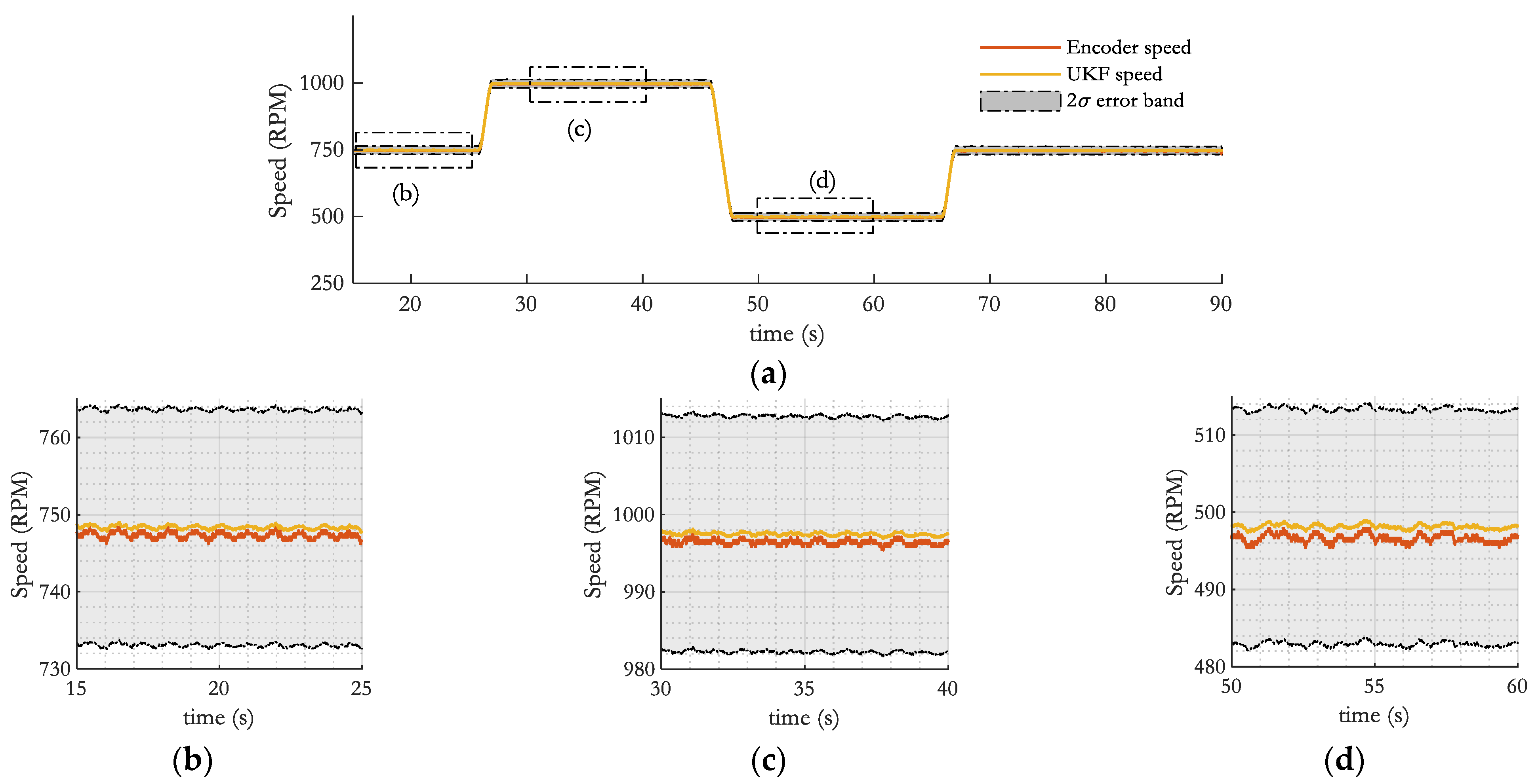
5.1. UKF Speed Filtering

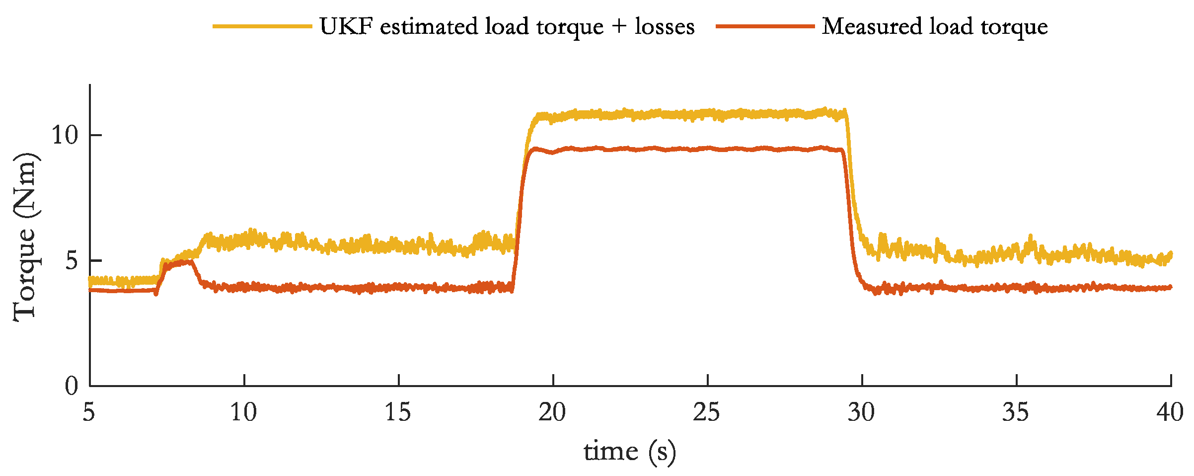
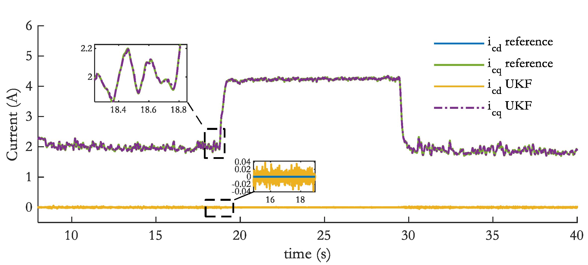
Results of the effective speed filtering capabilities of the UKF are shown in Figure 13. For this test, the machine is first started in IM mode at 40% load by short-circuiting the control winding phases. The control is then enabled for a speed reference of 750 RPM. At 17.6 s the load is increased to 100%. After the load step, the ripple on the UKF speed estimate decreases from 2.7% (or 20 RPM peak-to-peak) to less than 1% (or 6 RPM), thanks to the increased Signal to Noise Ratio (SNR) of the control winding current measurements, which are determinant for the UKF speed estimation. Finally, the difference between Figure 11 and Figure 13 can be explained by the difference in UKF covariance matrices which are tuned differently for the simulation and the real-time control. This is because of the difference between the model used in simulations, which is linear and does not include saturation and eddy current losses, and the real BDFRM prototype.

5.2. Load Rejection

When operating at constant speed, the implemented control system effectively rejects the sudden load variations. Load steps are applied from 40% to 100% and back, as depicted in Figure 14a. At the peak of the speed variation, the speed estimate error reaches around 6 RPM, less than 1 % of the nominal speed. The smoothed speed signals in Figure 14b,c show the performance of the UKF to follow the speed variations resulting from the load steps.

The load estimate, depicted in Figure 15, has a performant dynamic response, leading to relatively small speed variations, as shown in Figure 14. Moreover, as the speed control relies only on a P-controller, the feed forward of the load estimate lies at the base of the almost complete rejection of a potential steady-state error. Consequently, the overestimate of the measured torque indicates the presence of all sorts of losses not included in the model.

Finally, both control winding currents follow the imposed current references well, as even the ripples on the reference are followed by the controller of ${\mathrm{i}}_{\mathrm{c},\mathrm{q}}$, this is shown in Figure 16. This proves the performance of the implemented current control.

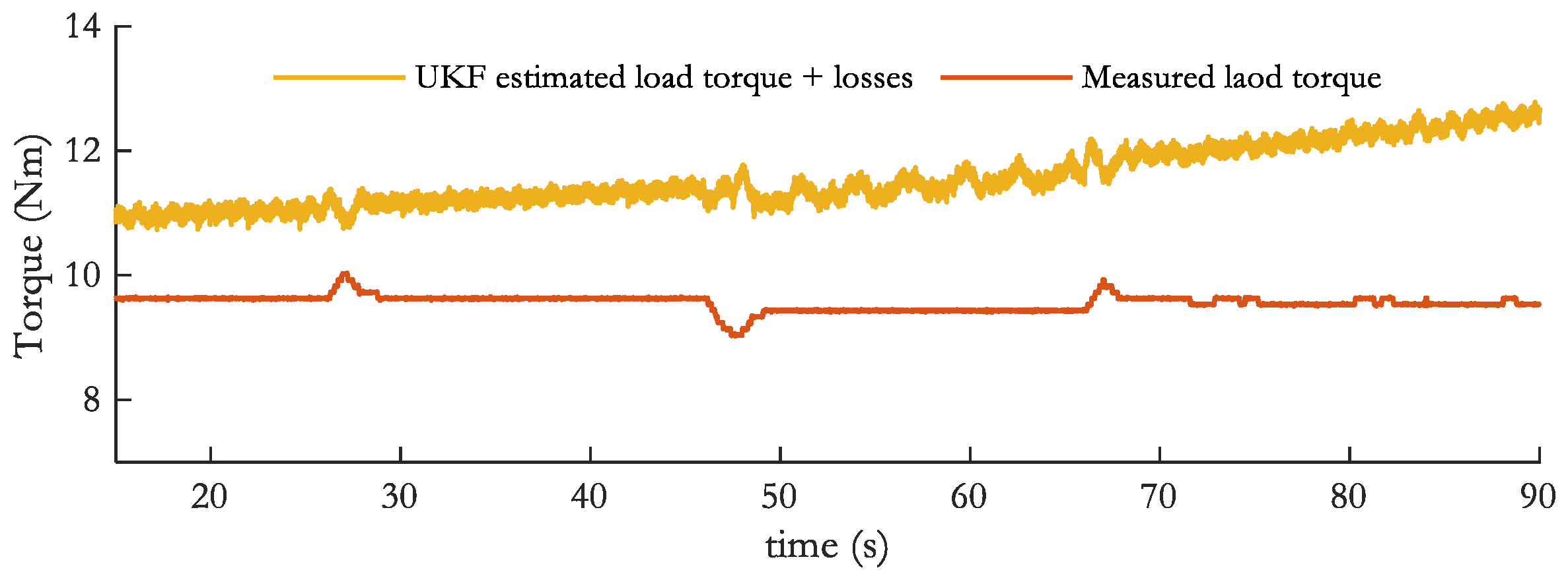
5.3. Variable Speed Operation

The variable speed performance of the proposed control method remains to be tested. To achieve this, the machine is nominally loaded at 9.5 Nm and a certain reference speed profile in the 500–1000 RPM speed range is applied, as this is the intended speed range for the intended application. The results, depicted in Figure 17, show that the steady-state error between the reference and the measured speed is approximately 0.35 % at 750 RPM and 1000 RPM, while it is approximately 0.7% at 500 RPM. Besides this, the steady-state error of the UKF speed estimation is below 0.3%.

The load estimate during the test is depicted in Figure 18 and it visibly drifts upward. This is due to the machine heating up, resulting in a winding resistance and, consequently, copper losses increase. Despite this, the control performance stays intact, meaning the UKF manages to correctly estimate the increasing losses. The grid winding phase resistance happened to be 32% higher than the initial one, indicating a rough temperature rise of at least 80 K during the test inside the machine. The temperature rise therefore also indicates a level of robustness of the presented control against a change in parameters.

5.4. Tuning of the UKF

The difficulty when implementing a Kalman filter is the correct allocation of the covariance matrices Q and R, a difficulty encountered by multiple reported works on Kalman filtering [40,67]. Even though some tuning methods exist [55,56,57], these add an additional layer of complexity. The matrix Q consists of the process noise (co)variances, these introduce the noise generated by the stochastic nature of the dynamic system and more importantly they contain the modelling errors. The modelling errors arise from all the assumptions made to construct the UKF BDFRM model, assumptions which are for example, the neglected iron losses, mechanical friction losses and the harmonic content in the airgap flux density.

Matrix R is the noise covariance matrix and can be estimated by studying the measurement errors, but simply using these estimates is usually not sufficient for the UKF to converge. The UKF covariance matrices Q and R, therefore, require some tuning effort, which implies setting the covariance elements such that satisfactory estimation performances are obtained.

In this paper, a certain tuning approach is introduced. First, the covariance matrices are considered as diagonal matrices, assuming the noises are uncorrelated and thus considering the covariances to be zero, thereby reducing the number of elements to tune. The tuning of variance depends on the nature of the related state variable and the level of ‘trust’ or ‘distrust’ that is allocated to a certain measurement or estimate. This approach proved to make the UKF converge and relatively accurately estimate the state variables. An important disclaimer is however that it remains a heuristic method and no evidence is to be found on the systematic performance of this tuning approach. Additionally, the variances of the same kind are kept equal, i.e., the four flux linkages share the same variance, same goes for the current measurements etc. Moreover, the tuning happens by setting a factor in front of the nominal chosen value of the standard deviation, the resulting diagonal matrices are given by Equations (64) and (65).

$$\mathbf{Q}=\mathrm{diag}\left(\left[{\left({\mathrm{k}}_{\mathsf{\lambda }}{\mathsf{\sigma }}_{\mathsf{\lambda }}\right)}^2{\mathbf{I}}_{1\mathrm{x}4}{\left({\mathrm{k}}_{{\mathsf{\omega }}_{\mathrm{r}}}{\mathsf{\sigma }}_{{\mathsf{\omega }}_{\mathrm{r}}}\right)}^2{\left({\mathrm{k}}_{{\mathsf{\theta }}_{\mathrm{r}}}{\mathsf{\sigma }}_{{\mathsf{\theta }}_{\mathrm{r}}}\right)}^2{\left({\mathrm{k}}_{{\mathrm{T}}_{\mathrm{load}}}{\mathsf{\sigma }}_{{\mathrm{T}}_{\mathrm{load}}}\right)}^2\right]\right)$$

(64)

$$\mathbf{R}=\mathrm{diag}\left(\left[{\left({\mathrm{k}}_{\mathrm{i}}{\mathsf{\sigma }}_{\mathrm{i}}\right)}^2{\mathsf{{\rm I}}}_{1\mathrm{x}4},{\left({\mathrm{k}}_{\mathrm{i}}{\mathsf{\sigma }}_{\mathrm{i}}\right)}^2,{\left({\mathrm{k}}_{\mathrm{enc}}{\mathsf{\sigma }}_{\mathrm{enc}}\right)}^2,{\left({\mathrm{k}}_{{\hat{\mathsf{\theta }}}_{\mathrm{r}}}{\mathsf{\sigma }}_{{\hat{\mathsf{\theta }}}_{\mathrm{r}}}\right)}^2\right]\right)$$

(65)

5.5. Encoderless Speed Estimation

Encoderless or sensorless speed control is attainable for the BDFRM as reported in [23,27,28,29,31,37]. The UKF proposed previously can be made encoderless by removing the speed measurement from the observation function h(x,u). The tuning of the covariance matrices is consequently much more difficult, as there is one measurement less available to assess and update the model predictions with. This results in more fragile stability of the implementation. Investigating the exact reasons behind these issues and their solutions could be considered for future work.

6. Conclusions

This paper proposes a new view on the machine model of the brushless doubly-fed reluctance machine (BDFRM), allowing the reuse of the existing model-based control system designs to operate the machine for variable speed applications. This is realized with a cascade control system in combination with an unscented Kalman filter (UKF) as state observer.

Based on the dynamic model in the grid winding field oriented (FO) frame, a cascade model-based control system was developed with an outer speed control loop and an inner current control loop. This cascaded control method is employed for a broad spectrum of different machines, such as the conventional synchronous and asynchronous machines. For the BDFRM, however, the proposed model-based control system was not developed and reported. Reasonable assumptions allowed simplifying the BDFRM model to become a model similar to the non-salient PMSM, with the grid winding flux linkage acting as PM flux. The model-based control system is approved for variable speed operation in simulation, assuming the use of ideal sensors.

To determine the load torque based on the model knowledge and to cope with the noisy measurements in a real BDFRM test-setup, a UKF is adopted as a state observer. Kalman filters can produce relatively accurate estimates of the state variables by fusing different kinds of clean and noisy signals. The UKF was chosen as the best KF option thanks to its ability to handle non-linear models with superior performance compared to the popular extended KF, while it also allows higher implementation flexibility.

The UKF implementation was first validated in simulation, followed by a successful implementation in real-time. The control system in combination with the UKF showed satisfactory performances, both in terms of accuracy and dynamic response, and the control requirements were successfully met. The proposed control system design is therefore validated experimentally. The UKF also proved capable of capturing an increase in losses due to a temperature rise in the windings. At this stage, future work could investigate sensorlsess speed control with the UKF, and on-line monitoring of phase resistances and other machine parameters.

References

1. Broadway, A.R.W. Cageless induction machine. Proc. Inst. Electr. Eng. 1971, 118, 1593. [Google Scholar] [CrossRef]
2. Wang, X.; McMahon, R.A.; Tavner, P.J. Design of the Brushless Doubly-Fed (Induction) Machine. In Proceedings of the IEEE International Electric Machines & Drives Conference, Antalya, Turkey, 3–5 May 2007. [Google Scholar]
3. Han, P.; Cheng, M.; Ademi, S.; Jovanovic, M.G. Brushless doubly-fed machines: Opportunities and challenges. Chin. J. Electr. Eng. 2018, 4, 1–17. [Google Scholar] [CrossRef]
4. Benômar, Y.; Croonen, J.; Verrelst, B.; Mierlo, J.V.; Hegazy, O. On Analytical Modeling of the Air Gap Field Modulation in the Brushless Doubly Fed Reluctance Machine. Energies 2021, 14, 2388. [Google Scholar] [CrossRef]
5. Han, P.; Zhang, J.; Cheng, M. Theoretical and Experimental Investigation of the Brushless Doubly-Fed Machine with a Multi-Barrier Rotor. In Proceedings of the 2018 IEEE Energy Conversion Congress and Exposition (ECCE), Portland, OR, USA, 23–27 September 2018. [Google Scholar]
6. Liang, F.; Xu, L.; Lipo, T.A. d-q analysis of a variable speed doubly ac excited reluctance motor. Electr. Mach. Power Syst. 1991, 19, 125–138. [Google Scholar] [CrossRef]
7. Wang, F.; Zhang, F.; Xu, L. Parameter and performance comparison of doubly fed brushless machine with cage and reluctance rotors. IEEE Trans. Ind. Appl. 2002, 38, 1237–1243. [Google Scholar] [CrossRef]
8. Jovanovic, M.G.; Betz, R.E.; Yu, J. The use of doubly fed reluctance machines for large pumps and wind turbines. IEEE Trans. Ind. Appl. 2002, 38, 1508–1516. [Google Scholar] [CrossRef]
9. Jovanovic, M.; Betz, R. Power factor control using brushless doubly fed reluctance machines. In Proceedings of the Conference Record of the 2000 IEEE Industry Applications Conference, Thirty-Fifth IAS Annual Meeting and World Conference on Industrial Applications of Electrical Energy (Cat. No. 00CH37129), Rome, Italy, 8–12 October 2000; pp. 523–530. [Google Scholar]
10. Xu, L.; Wang, F. Comparative study of magnetic coupling for a doubly fed brushless machine with reluctance and cage rotors. In Proceedings of the IAS’97. Conference Record of the 1997 IEEE Industry Applications Conference Thirty-Second IAS Annual Meeting, New Orleans, LA, USA, 5–9 October 1997; pp. 326–332. [Google Scholar]
11. Xu, L.; Zhen, L.; Kim, E.-H. Field orientation control of a doubly excited brushless reluctance machine. In Proceedings of IAS’96. Conference Record of the 1996 IEEE Industry Applications Conference Thirty-First IAS Annual Meeting, San Diego, CA, USA, 6–10 October 1996; pp. 319–325. [Google Scholar]
12. Dorrell, D.G.; Jovanovic, M. On the Possibilities of Using a Brushless Doubly-Fed Reluctance Generator in a 2 MW Wind Turbine. In Proceedings of the 2008 IEEE Industry Applications Society Annual Meeting, Edmonton, AB, Canada, 5–9 October 2008; pp. 1–8. [Google Scholar]
13. Protsenko, K.; Xu, D. Modeling and Control of Brushless Doubly-Fed Induction Generators in Wind Energy Applications. In Proceedings of the APEC 07—Twenty-Second Annual IEEE Applied Power Electronics Conference and Exposition, Anaheim, CA, USA, 25 Febuary–1 March 2007; pp. 529–535. [Google Scholar]
14. Gorti, B.; Zhou, D.; Spée, R.; Alexander, G.; Wallace, A. Development of a brushless doubly-fed machine for a limited-speed pump drive in a waste-water treatment plant. In Proceedings of the 1994 IEEE Industry Applications Society Annual Meeting, Denver, CO, USA, 2–6 October 1994; pp. 523–529. [Google Scholar]
15. Xu, L.; Tang, Y. A novel wind-power generating system using field orientation controlled doubly-excited brushless reluctance machine. In Proceedings of the Conference Record of the 1992 IEEE Industry Applications Society Annual Meeting, Houston, TX, USA, 4 October 1992; pp. 408–413. [Google Scholar]
16. Agrawal, S.; Province, A.; Banerjee, A. An Approach to Maximize Torque Density in a Brushless Doubly Fed Reluctance Machine. IEEE Trans. Ind. Appl. 2020, 56, 4829–4838. [Google Scholar] [CrossRef]
17. Jovanovic, M.G.; Betz, R.E.; Yu, J.; Levi, E. Aspects of vector and scalar control of brushless doubly fed reluctance machines. In Proceedings of the 4th IEEE International Conference on Power Electronics and Drive Systems, IEEE PEDS 2001-Indonesia. Proceedings (Cat. No. 01TH8594), Denpasar, Indonesia, 25 October 2001; pp. 461–467. [Google Scholar]
18. Hassan, M.; Jovanovic, M. Improved scalar control using flexible DC-Link voltage in brushless doubly-fed reluctance machines for wind applications. In Proceedings of the 2012 2nd International Symposium on Environment Friendly Energies and Applications, Newcastle upon Tyne, UK, 25–27 June 2012; pp. 482–487. [Google Scholar]
19. Taluo, T.; Ristić, L.; Jovanović, M. Performance Analysis of Brushless Doubly Fed Reluctance Machines. In Proceedings of the 2019 20th International Symposium on Power Electronics (Ee), Novi Sad, Serbia, 23–26 October 2019; pp. 1–6. [Google Scholar]
20. Ademi, S.; Jovanović, M.G. Vector Control Methods for Brushless Doubly Fed Reluctance Machines. IEEE Trans. Ind. Electron. 2015, 62, 96–104. [Google Scholar] [CrossRef]
21. Jovanovic, M.; Yu, J.; Levi, E. Direct Torque Control of Brushless Doubly Fed Reluctance Machines. Electr. Power Compon. Syst. 2004, 32, 941–958. [Google Scholar] [CrossRef]
22. Jovanovic, M. Control of brushless doubly-fed reluctance motors. In Proceedings of the IEEE International Symposium on Industrial Electronics, 2005. ISIE 2005, Dubrovnik, Croatia, 20–23 June 2005; pp. 1667–1672. [Google Scholar]
23. Jovanovic, M.; Yu, J.; Levi, E. A doubly-fed reluctance motor drive with sensorless direct torque control. In Proceedings of the IEEE International Electric Machines and Drives Conference, 2003. IEMDC’03, Madison, WI, USA, 1–4 June 2003; pp. 1518–1524. [Google Scholar]
24. Kiran, K.; Das, S.; Singh, D. Model predictive field oriented speed control of brushless doubly-fed reluctance motor drive. In Proceedings of the 2018 International Conference on Power, Instrumentation, Control and Computing (PICC), Thrissur, India, 18–20 January 2018; pp. 1–6. [Google Scholar]
25. Kiran, K.; Das, S. Variable speed operation of brushless doubly fed reluctance machine drive using model predictive current control technique. IEEE Trans. Power Electron. 2020, 35, 8396–8404. [Google Scholar] [CrossRef]
26. Jovanovic, M.G.; Dorrell, D.G. Sensorless control of brushless doubly-fed reluctance machines using an angular velocity observer. In Proceedings of the 2007 7th International Conference on Power Electronics and Drive Systems, Bangkok, Thailand, 27–30 November 2007; pp. 717–724. [Google Scholar]
27. Ademi, S.; Jovanović, M.G.; Chaal, H.; Cao, W. A new sensorless speed control scheme for doubly fed reluctance generators. IEEE Trans. Energy Convers. 2016, 31, 993–1001. [Google Scholar] [CrossRef]
28. Kiran, K.; Das, S. Implementation of reactive power-based MRAS for sensorless speed control of brushless doubly fed reluctance motor drive. IET Power Electron. 2017, 11, 192–201. [Google Scholar] [CrossRef]
29. Kiran, K.; Das, S.; Kumar, M.; Sahu, A. Sensorless Speed Control of Brushless Doubly-Fed Reluctance Motor Drive using Secondary Flux based MRAS. Electr. Power Compon. Syst. 2018, 46, 701–715. [Google Scholar] [CrossRef]
30. Kiran, K.; Das, S.; Sahu, A. Sensorless speed estimation and control of brushless doubly-fed reluctance machine drive using model reference adaptive system. In Proceedings of the 2016 IEEE International Conference on Power Electronics, Drives and Energy Systems (PEDES), Thiruvananthapuram, India, 14–17 December 2016; pp. 1–6. [Google Scholar]
31. Jovanovic, M. Sensored and sensorless speed control methods for brushless doubly fed reluctance motors. IET Electr. Power Appl. 2009, 3, 503–513. [Google Scholar] [CrossRef]
32. Betz, R.E.; Jovanović, M.G. Introduction to the Space Vector Modeling of the Brushless Doubly Fed Reluctance Machine. Electr. Power Compon. Syst. 2003, 31, 729–755. [Google Scholar] [CrossRef]
33. Quang, N.P.; Dittrich, J.-A. Vector Control of Three-Phase AC Machines; Springer: Berlin/Heidelberg, Germany, 2008; Volume 2, Available online: https://0-link-springer-com.brum.beds.ac.uk/book/10.1007/978-3-662-46915-6 (accessed on 6 December 2021).
34. Takahashi, I.; Noguchi, T. A New Quick-Response and High-Efficiency Control Strategy of an Induction Motor. IEEE Trans. Ind. Appl. 1986, IA-22, 820–827. [Google Scholar] [CrossRef]
35. Song, W.K.; Dorrell, D.G. Implementation of improved direct torque control method of brushless doubly-fed reluctance machines for wind turbine. In Proceedings of the 2014 IEEE International Conference on Industrial Technology (ICIT), Busan, Korea, 26 February–1 March 2014; pp. 509–513. [Google Scholar]
36. Chaal, H.; Jovanovic, M. Improved Direct Torque Control Using Kalman Filter: Application to a Doubly-Fed Machine. 2009. Available online: https://www.semanticscholar.org/paper/Improved-direct-torque-control-using-Kalman-filter%3A-Chaal-Jovanovi%C4%87/e159a090d3dc9c627698a9e126c8ff93e9459dff#citing-papers (accessed on 29 November 2021).
37. Kumar, M.; Das, S.; Kiran, K. Sensorless Speed Estimation of Brushless Doubly-Fed Reluctance Generator Using Active Power Based MRAS. IEEE Trans. Power Electron. 2019, 34, 7878–7886. [Google Scholar] [CrossRef]
38. Betz, R.E.; Jovanovic, M. Introduction to Brushless Doubly Fed Reluctance Machines—The Basic Equations; Aalborg University: Aalborg, Denmark, 1998. [Google Scholar] [CrossRef]
39. Betz, R.E.; Jovanovic, M.G. Brushless Doubly Fed Reluctance Machines—A Tutorial. 2003. Available online: https://citeseerx.ist.psu.edu/viewdoc/download?doi=10.1.1.565.8777&rep=rep1&type=pdf (accessed on 29 November 2021).
40. Terorde, G. Electrical Drives and Control Techniques; ACCO: Leuven, Belgium, 2004. [Google Scholar]
41. Umland, J.W.; Safiuddin, M. Magnitude and symmetric optimum criterion for the design of linear control systems: What is it and how does it compare with the others? IEEE Trans. Ind. Appl. 1990, 26, 489–497. [Google Scholar] [CrossRef]
42. Papadopoulos, K.G. PID Controller Tuning Using the Magnitude Optimum Criterion; Springer: Berlin/Heidelberg, Germany, 2015. [Google Scholar]
43. Maybeck, P.S. Stochastic Models, Estimation, and Control; Academic Press: Cambridge, MA, USA, 1979. [Google Scholar]
44. Anderson, B.D.; Moore, J.B. Optimal Filtering; Courier Corporation: Chelmsfors, MA, USA, 2012. [Google Scholar]
45. Julier, S.J.; Uhlmann, J.K. New extension of the Kalman filter to nonlinear systems. In Signal Processing, Sensor Fusion, and Target Recognition VI; International Society for Optics and Photonics: Bellingham, WA, USA, 1997; pp. 182–193. [Google Scholar]
46. Alonge, F.; Cangemi, T.; D’Ippolito, F.; Fagiolini, A.; Sferlazza, A. Convergence analysis of extended Kalman filter for sensorless control of induction motor. IEEE Trans. Ind. Electron. 2014, 62, 2341–2352. [Google Scholar] [CrossRef]
47. Yildiz, R.; Barut, M.; Demir, R. Extended Kalman filter based estimations for improving speed-sensored control performance of induction motors. IET Electr. Power Appl. 2020, 14, 2471–2479. [Google Scholar] [CrossRef]
48. Niedermayr, P.; Alberti, L.; Bolognani, S.; Abl, R. Implementation and experimental validation of ultra-high speed PMSM sensor-less control by means of extended Kalman filter. IEEE J. Emerg. Sel. Top. Power Electron. 2020, 1. [Google Scholar] [CrossRef]
49. Shi, K.; Chan, T.; Wong, Y.; Ho, S.L. Speed estimation of an induction motor drive using an optimized extended Kalman filter. IEEE Trans. Ind. Electron. 2002, 49, 124–133. [Google Scholar] [CrossRef] [Green Version]
50. Wan, E.A.; Van Der Merwe, R. The unscented Kalman filter for nonlinear estimation. In Proceedings of the IEEE 2000 Adaptive Systems for Signal Processing, Communications, and Control Symposium (Cat. No. 00EX373), Lake Louise, AB, Canada, 4 October 2000; pp. 153–158. [Google Scholar]
51. Giannitrapani, A.; Ceccarelli, N.; Scortecci, F.; Garulli, A. Comparison of EKF and UKF for spacecraft localization via angle measurements. IEEE Trans. Aerosp. Electron. Syst. 2011, 47, 75–84. [Google Scholar] [CrossRef]
52. He, H.; Qin, H.; Sun, X.; Shui, Y. Comparison Study on the Battery SoC Estimation with EKF and UKF Algorithms. Energies 2013, 6, 5088–5100. [Google Scholar] [CrossRef]
53. Kurt-Yavuz, Z.; Yavuz, S. A comparison of EKF, UKF, FastSLAM2. 0, and UKF-based FastSLAM algorithms. In Proceedings of 2012 IEEE 16th International Conference on Intelligent Engineering Systems (INES), Lisabon, Portugal, 13–15 June 2012; pp. 37–43. [Google Scholar]
54. Van Der Merwe, R.; Wan, E.A. The square-root unscented Kalman filter for state and parameter-estimation. In Proceedings of the 2001 IEEE International Conference on Acoustics, Speech, and Signal Processing, Proceedings (Cat. No. 01CH37221), Salt Lake City, UT, USA, 7–11 May 2001; pp. 3461–3464. [Google Scholar]
55. Åkesson, B.M.; Jørgensen, J.B.; Poulsen, N.K.; Jørgensen, S.B. A generalized autocovariance least-squares method for Kalman filter tuning. J. Process Control 2008, 18, 769–779. [Google Scholar] [CrossRef]
56. Loebis, D.; Sutton, R.; Chudley, J.; Naeem, W. Adaptive tuning of a Kalman filter via fuzzy logic for an intelligent AUV navigation system. Control Eng. Pract. 2004, 12, 1531–1539. [Google Scholar] [CrossRef]
57. Åkesson, B.M.; Jørgensen, J.B.; Poulsen, N.K.; Jørgensen, S.B. A tool for kalman filter tuning. In Computer Aided Chemical Engineering; Elsevier: Amsterdam, The Netherlands, 2007; Volume 24, pp. 859–864. [Google Scholar]
58. Li, H. A Brief Tutorial On Recursive Estimation: Examples From Intelligent Vehicle Applications (Part III). 2014. Available online: https://hal.archives-ouvertes.fr/hal-01020546v1 (accessed on 29 November 2021).
59. Betz, R.E.; Jovanovic, M.G. Theoretical analysis of control properties for the brushless doubly fed reluctance machine. IEEE Trans. Energy Convers. 2002, 17, 332–339. [Google Scholar] [CrossRef]
60. Ghahremani, E.; Kamwa, I. Dynamic State Estimation in Power System by Applying the Extended Kalman Filter With Unknown Inputs to Phasor Measurements. IEEE Trans. Power Syst. 2011, 26, 2556–2566. [Google Scholar] [CrossRef]
61. Terejanu, G.A. Unscented Kalman Filter Tutorial; Univerity of Buffalo: Buffalo, NY, USA, 2011. [Google Scholar]
62. Dash, P.K.; Jena, R.; Panda, G.; Routray, A. An extended complex Kalman filter for frequency measurement of distorted signals. IEEE Trans. Instrum. Meas. 2000, 49, 746–753. [Google Scholar] [CrossRef] [Green Version]
63. Dash, P.; Pradhan, A.; Panda, G. Frequency estimation of distorted power system signals using extended complex Kalman filter. IEEE Trans. Power Deliv. 1999, 14, 761–766. [Google Scholar] [CrossRef] [Green Version]
64. Nanda, S.; Dash, P.K. A Gauss–Newton ADALINE for dynamic phasor estimation of power signals and its FPGA implementation. IEEE Trans. Instrum. Meas. 2016, 67, 45–56. [Google Scholar] [CrossRef]
65. Halbwachs, D.; Wira, P.; Mercklé, J. Adaline-based approaches for time-varying frequency estimation in power systems. IFAC Proc. Vol. 2009, 42, 31–36. [Google Scholar] [CrossRef]
66. Dash, P.; Swain, D.; Routray, A.; Liew, A. An adaptive neural network approach for the estimation of power system frequency. Electr. Power Syst. Res. 1997, 41, 203–210. [Google Scholar] [CrossRef]
67. Schneider, R.; Georgakis, C. How To NOT Make the Extended Kalman Filter Fail. Ind. Eng. Chem. Res. 2013, 52, 3354–3362. [Google Scholar] [CrossRef]
Figure 1. Schematic of the BDFRM drive under consideration.
Energies 14 08222 g001
Figure 2. Cascade feedback speed control of electrical machines.
Energies 14 08222 g002
Figure 3. Equivalent circuit of the control winding in a FO dq-reference frame.
Energies 14 08222 g003
Figure 4. Control system for inverter current control at the control winding of the BDFRM.
Energies 14 08222 g004
Figure 5. (a) Control winding current control loop. (b) Torque control loop with the equivalent plant model of the BDFRM and the inverter + ADC/DAC.
Energies 14 08222 g005
Figure 6. Speed controller with load compensation.
Energies 14 08222 g006
Figure 7. (a) Speed profile over the speed range 500–1000 RPM for a BDFRM with 6 rotor poles, with a speed rate of change of 300 RPM/s. (b) Start-up of the BDFRM in induction mode. (c) Reference and actual speed during ramp-up.
Energies 14 08222 g007
Figure 8. (a) Response of control winding current controllers during the simulated speed profile. (b) Zoom in around the load step. (c) Zoom in around the ramp up from 750 RPM to 1000 RPM. Current amplitudes are expressed in a power invariant dq-reference frame.
Energies 14 08222 g008aEnergies 14 08222 g008b
Figure 9. (a) Mean and covariance propagation through a dynamic system. (b) Linear approximation adopted by the EKF. (c) Unscented transformation of sample points and posterior calculation of mean and covariance.
Energies 14 08222 g009
Figure 10. Estimation of the dq grid winding current components based on the numerical integration of the grid winding flux linkage in the stationary frame.
Energies 14 08222 g010
Figure 11. (a) Simulation results of the proposed speed control system with the UKF as an observer for speed and load torque. (b) Zoom on the load step. (c) Zoom on the speed ramp-up.
Energies 14 08222 g011
Figure 12. (a) Assembled stator and skewed rotor of the BDFRM prototype under test, (b) single flux guide and (c) setup for testing the prototype at different speeds [4].
Energies 14 08222 g012
Figure 13. Raw signal from the shaft encoder and the estimated UKF speed.
Energies 14 08222 g013
Figure 14. (a) Measured and estimated shaft speed, with the error band of the UKF estimate, during the load rejection test of the proposed controller at 750 RPM with a zoom on the (b) loading and (c) unloading step. The curves are smoothed over 0.3 s.
Energies 14 08222 g014
Figure 15. Estimated load torque and losses and measured torque during the load rejection test. The measured torque is smoothed over 0.3 s.
Energies 14 08222 g015
Figure 16. Control winding current controller response during the load rejection test. The curves are smoothed over 0.1 s. Current amplitudes are expressed in a power invariant dq-reference frame.
Energies 14 08222 g016
Figure 17. (a) Speed control results for a speed variation rate of 300 RPM/s under 100% load conditions with a zoom on reference speeds (b) 750 RPM, (c) 1000 RPM and (d) 500 RPM.
Energies 14 08222 g017
Figure 18. Estimated and measured torque during the speed profile test.
Energies 14 08222 g018