Exploitation of a New Short-Term Multimodel Photovoltaic Power Forecasting Method in the Very Short-Term Horizon to Derive a Multi-Time Scale Forecasting System

Abstract

The relentless spread of photovoltaic production drives searches of smart approaches to mitigate unbalances in power demand and supply, instability on the grid and ensuring stable revenues to the producer. Because of the development of energy markets with multiple time sessions, there is a growing need of power forecasting for multiple time steps, from fifteen minutes up to days ahead. To address this issue, in this study both a short-term-horizon of three days and a very-short-term-horizon of three hours photovoltaic production forecasting methods are presented. The short-term is based on a multimodel approach and referred to several configurations of the Analog Ensemble method, using the weather forecast of four numerical weather prediction models. The very-short-term consists of an Auto-Regressive Integrated Moving Average Model with eXogenous input (ARIMAX) that uses the short-term power forecast and the irradiance from satellite elaborations as exogenous variables. The methods, applied for one year to four small-scale grid-connected plants in Italy, have obtained promising improvements with respect to refence methods. The time horizon after which the short-term was able to outperform the very-short-term has also been analyzed. The study also revealed the usefulness of satellite data on cloudiness to properly interpret the results of the performance analysis.

1. Introduction

Energy sector has undergone rapid and substantial transformations during the last decade, both in terms of energy production and consumption. The increase in global energy demand on the one hand and the necessity to mitigate the dramatic effects of climate change, on the other hand, have forced researchers, policymakers and economists to look for new energy production systems, less dependent on exhaustible sources, more efficient and characterized by low emissions of greenhouse components into the atmosphere. Ambitious commitments have been taken during the United Nations Climate Change Conference (COP21) in 2015, to limit global warming to well below 2° Celsius. In order to reach this result, a decarbonization in the energy production system is underway. Green energy incentives and the progressive and continuous decrease of solar and wind costs [1], have led to a huge deployment of renewable plants worldwide. 2019 marked a record with 200 GW of renewable power added globally [1], 115 of which were solar installations. The beginning of 2020, despite the global reduction in energy demand, due to COVID-19, saw an increase in renewable power demand [2]. In the same period, a record in the share of solar and wind production in the electricity demand was experienced in many countries, undermining the safety and the stability of the transmission and distribution grid, due to the inherent variability of these sources. It is well known, in fact, that the production of solar and wind plants is mainly affected by weather conditions, causing sudden variations in production profiles and requiring rapid actions by grid operators in order to mitigate imbalances between demand and supply of energy. This results in an increase of flexible energy reserve to address imbalances and additional uncertainty in the energy market. By means of an accurate forecasting of power production, the benefits of using renewable sources over fossil-fired power plants will increase to an ever-greater extent. In addition to undoubted advantages for the environment, in terms of avoided CO₂ emissions, solar renewable production is profitable for the producer first of all because the fuel is free and inexhaustible. Furthermore, in many countries there are lots of incentives to promote renewable energy projects. For example, in Europe the Cohesion Fund allocated a total of €63.4 billion to promote sustainable development between 2014 and 2020 in some European countries and around €5.9 billion have been devoted towards energy research and innovation projects in the European Union Horizon 2020 program. At present, the convenience in using fossil-fired sources appears to result from the possibility to tune the production according to the short-time power demand. Actually, with an accurate production forecast, updated several times a day, it is possible to optimize the management of ancillary systems to supply energy in case of demand peaks, allowing to choose the most convenient production system according to the current scenario of power demand and supply. Accurate forecasting also allows for better management of storage systems that can be coupled with solar plants, making it more profitable. Finally, in many countries, penalties are applied when inaccurate power predictions plans are submitted, and the economic value of accurate forecasting has been investigated by Antonanzas et al. [3] and Reindl et al. [4].

The variability of nonprogrammable renewable sources affects different time scales, with several impacts. For example, the precise knowledge on the future renewable energy (RE) profile in the range of minutes is particularly beneficial for real time dispatch operation, storage control, grid stability management [5]. The variability in the next few hours is closely related to energy trading in the intraday market, along with the management of storage devices and dispatching operations [6]. The RE profile for the subsequent days mainly applies to planning purposes and to formulate bids for electricity markets [4,7].

According to the forecast horizon, various approaches have been developed up to now, using different types of input data. Recent comprehensive reviews of PhotoVoltaic (PV) solar power forecasting techniques can be obtained from Das et al. [5], Mellit et al. [8], Ahmed et al. [9]. In particular, in the review by Ahmed et al. [9] there is a discussion on the terms used to define the forecast horizon and there is an attempt to classify the forecasting techniques in categories: persistence forecasting, physical models, statistical techniques. It is important to note that the expression “physical approach” is often used with different meaning. In the same review [9], for example, it relates to the use of Numerical Weather Prediction models (NWP) to forecast the meteorological variables affecting renewable production. It is necessary to be aware that NWP do not provide production forecasts, but they solve the integrodifferential equations describing the state of the atmosphere and soil/land/sea/ atmosphere interactions at different spatial scales. As output, they also predict the values of the meteorological variables affecting RE production. It is always necessary a postprocessing to convert weather information in production forecast. In this case, the final power forecast will be derived with two possible ways: by means of a statistical technique that uses in input NWP forecasts, such as Artificial Neural Network (ANN), Support Vector Machine (SVM) and so forth, or by using the same information to feed a specific model of the plant, describing system size, module and array type, system losses, inverter efficiency and so on. Some authors refer to the latter type of model, that is a detailed simulation of the real plant, as the physical approach [10]. Therefore, it is necessary to pay close attention to the meaning of the words used in this field by authors with different backgrounds. There are many and varied techniques exploited so far to derive PV power forecasting. The simplest one is the persistence forecast, which is considered an accurate and cost-effective forecasting system in the range of 0–15 min ahead by many authors, such as Dutta et al. [11], Barbieri et al. [12] and Zhou et al. [13]. Another group of forecasting systems includes time series based forecasting techniques, such as exponential smoothing methods, autoregressive moving average (ARMA), autoregressive integrated moving average (ARIMA), as reported by Pedro et al. [14], Ahmad et al. [15], Nobre et al. [16]. These methods predict the forthcoming value of a variable by evaluating the pattern of the same variable in the past They are characterized by the absence of exogenous inputs. ARIMA models, with respect to ARMA models, have the capability of clipping nonstationary values from the data. These methods have been implemented for both sub-hourly and day-ahead forecasting horizons. ARIMA is often used as reference method. Time series methods have the undoubted advantage of being very fast. However, the main drawback is the lack of physical modelling during the forecasting process, such as the absence of weather information. This issue can be addressed with the multivariate versions of time series models, such as the Auto-Regressive Integrated Moving Average Model with eXogenous input (ARIMAX). To the best of authors’ knowledge, only few authors have explored the latter methodology for PV power forecasting applications, such as Zhou et al. [13], Bacher et al. [17], Perez-Mora et al. [18] and Li et al. [19], even if it seems a cost-effective forecasting system with good performances.

The most popular methods used in PV power forecasting exploit machine learning (ML) techniques. This approach refers to the ability of computers to learn from experience, without being programmed by human beings, as described by Samuel A.L. [20]. They include Artificial Neural Networks (ANN) with their ability to approximate nonlinear functions. The ANN architecture consists of a network of connected artificial neurons in different layers: the input, the hidden (multiple levels are possible), and the output layer. The neuron consists of input(s), net function, transfer function, and output(s). There are lots of different types of ANN with different architectures used to derive PV power forecasting [14,21,22]. A subset of ML techniques is the Deep Learning (DL), referring to the ability of deep neural networks of learning from voluminous input data and numerous hidden layers, as specified by Deng and Yu [23]. Convolutional Neural Network (CNN) [24], Long Short Term Memory (LSTM) [13,25,26], multilayer perceptron (MLP) [27], recurrent neural network (RNN) [28,29] are the principal DL methods. A specific recent review of ML and DL methods applied to PV power forecasting is presented by Mellit et al. [8]. These methods are considered promising and accurate when implemented with a large training dataset. They often require pretreatments of the dataset, to exclude outliers and wrong data. They may experience overfitting problems and they are computation intensive. They need to be retrained when new data are available, therefore, for online application, for example with constant updates of the forecast during the day, they may not be the most efficient solution.

Another approach consists in the probabilistic forecast. With the probabilistic approach the output consists of a distribution of probability of the future values of power. The research in the probabilistic forecast of solar power production is generally considered immature at present. A review regarding this approach has been made by Van der Meer et al. [30]. The most popular probabilistic forecasting models are quantile regression-based methods, presented by Lauret et al. [31], and simulating predictors used by Kim et al. [32]. The probabilistic forecasting is often obtained by feeding simulated explanatory weather scenarios into a deterministic forecasting model. In this regard a recent work by Sun et al. [33] pointed out the importance of considering the correlation among different explanatory weather variables. This analysis can be performed when historical measured and forecasted weather data are available. In many countries the availability of weather measurements is rather limited, in part because they are managed by different companies and they are not available free of charge. Radiation measurements, in particular, are obtained from costly instruments and they are therefore even rarer. An alternative probabilistic approach that does not require weather measurements consists in the Analog Ensemble, implemented by Alessandrini et al. [34]. The Analog Ensemble (AnEn) is a statistical technique that uses the weather forecast predictors to identify the past events more similar to the current forecast. Once selected the time in which similar weather forecast have occurred, a distribution of the forecasting variable is created using the past measurements of that variable recorded in those past times.

Up to now researchers have been mainly focused to derive the most accurate power forecasting tool for a specific forecast horizon, such as the very-short-term (15–180 min ahead) or the short-term (up to 72 h ahead), according to the final application of the forecasting.

At the moment, the interest in accurate production forecasts for multiple time frames, from few minutes in advance, till some days ahead, is growing more and more, especially for solar, due to its ever-increasing penetration in electricity grids. More and more often, photovoltaic plants are coupled with storage systems, in order to store surplus energy and eventually use the hybrid system for balancing purposes. Innovative technological solutions are being developed in this field, such as new photovoltaic panels with integrated lithium accumulators as suggested by Poulek et al. [35]. In this case, for the optimal management of the system, a real time PV power forecasting is necessary, especially to deal with ramps, but it is also important to know the production profile of the following days, in order to operate a smart management of the storage and because producers are often asked to supply the day-ahead production plan to prevent serious stability issues on the grid. Furthermore, the same producer may be interested in participating in both the intra-day and day-ahead energy market. This requirement is catching on in many countries, also because of the creation of aggregators of distributed solar producers, participating directly in electricity markets.

As regards the primary source, an analysis on the performance of different irradiance forecasting methods to varying of the spatial-time scale is reported by Diagne et al. [36]. On the basis of the fact that the main factor affecting PV production is the solar irradiation, as reported by Diagne et al. [36], Cai et al. [37], Liu et al. [38], it is usual to transfer the considerations derived from irradiance forecasting studies also in the PV forecasting field, but a corresponding analysis of the variation of the PV power forecasting performances when the forecasting horizon changes from few minutes until days ahead has not been performed yet.

On the other hand, the research in multiple time frames prediction is immature and according to Mellit et al. [8] the multistep prediction is a current challenge in the PV field. Mishra et al. [39] proposed an RNN-based approach to forecast the PV production from one hour till 4 h ahead. The method was implemented using lots of observed weather variables. It achieved low root mean square errors across all the forecasting time-horizons and brought out the relevance of multi-time horizon forecasting for industrial applications. This method has the drawback of the necessity of observed weather data, often not available close to the plant and covers a limited range of forecast. A more extended multistep prediction has been addressed by Carriere et al. [40], with a PV power forecasting spanning from five minutes till thirty-six hours ahead.

They have highlighted the reasons behind a PV power forecasting covering multiple time frames and proposed an approach based on the AnEn technique. In their work the same model was used along the time, fed with observed data, NWP forecasts and satellite information. The system was tested on large PV plants with performances comparable with the state-of-the-art approaches developed for specific time horizons. The strength of this approach is to use a single method for all the forecast horizons, even if this condition could lead to less accuracy for specific timeframe, with respect to use different methods, for different horizons.

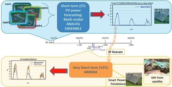
In this work the implementation of a multistep PV power forecasting tool, covering the horizons from 15 min to three days ahead with a time resolution of fifteen minutes, has been addressed in a different way, by exploiting two different methods, one devoted to deriving an accurate forecast for the short-term (ST) horizon, till three days ahead and another one for the very-short-term horizon (VST), covering the period from 15 min till three hours in advance.

The ST forecasting is an original method, based on a multimodel approach, made of different configurations of an Analog Ensemble, fed with the weather forecast derived from various NWP models. The very-short-term PV power forecast is generated based on ARIMAX method, using the PV forecast derived from the ST prediction as explanatory variable.

With regard to the methods, AnEn has already revealed its strength in previous applications on PV power forecasting, compared to other state of art methods, such as quantile regression, as confirmed by Alessandrini et al. [34] and with respect to hybrid methods combining k-Nearest Neighbors and Quantile Regression Forest and a Multi-Layer Perceptron neural network, as studied in the benchmark on regional PV power forecasting models by Pierro et al. [41]. In addition to its performance, another advantage of this method is that it requires minimal computational resources. The novelty of the AnEn used in this work consists in the multimodel approach, derived from different configurations of the AnEn, as well as the use of more than just one NWP prediction model in input to the AnEn.

For the VST, the ARIMAX has been chosen because it is a fast algorithm, therefore it is appropriate for online use. It is able to rapidly adapt to changes in operational production, such as fell in production due to breaks of arrays or degradations of inverters. It does not need to be re-trained when new measurements are available. As regards its reliability, even though it has been under-exploited so far, it has proven to be able to provide better prediction performance than an NN model by Li et al. [19]. The ARIMAX implemented in this work has the peculiarity of using the output of the ST forecast as explanatory variable, in addition to two more exogenous variables, i.e., irradiation from satellite data and a smart power persistence of the PV power.

The main originality of the work lies in the exploitation of the results of the ST in the VST, as well as the use of a multimodel approach to improve the performance of the ST. The performance variations of the multimodel ST and VST along the entire forecasting time have been evaluated, in order to detect the time horizon after which the ST could outperform the VST.

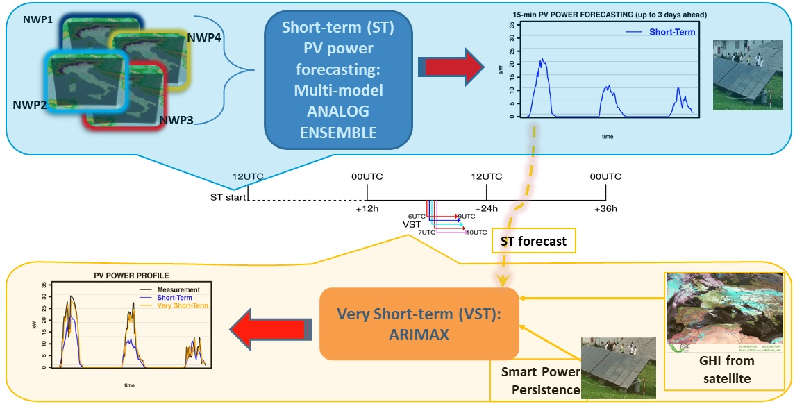
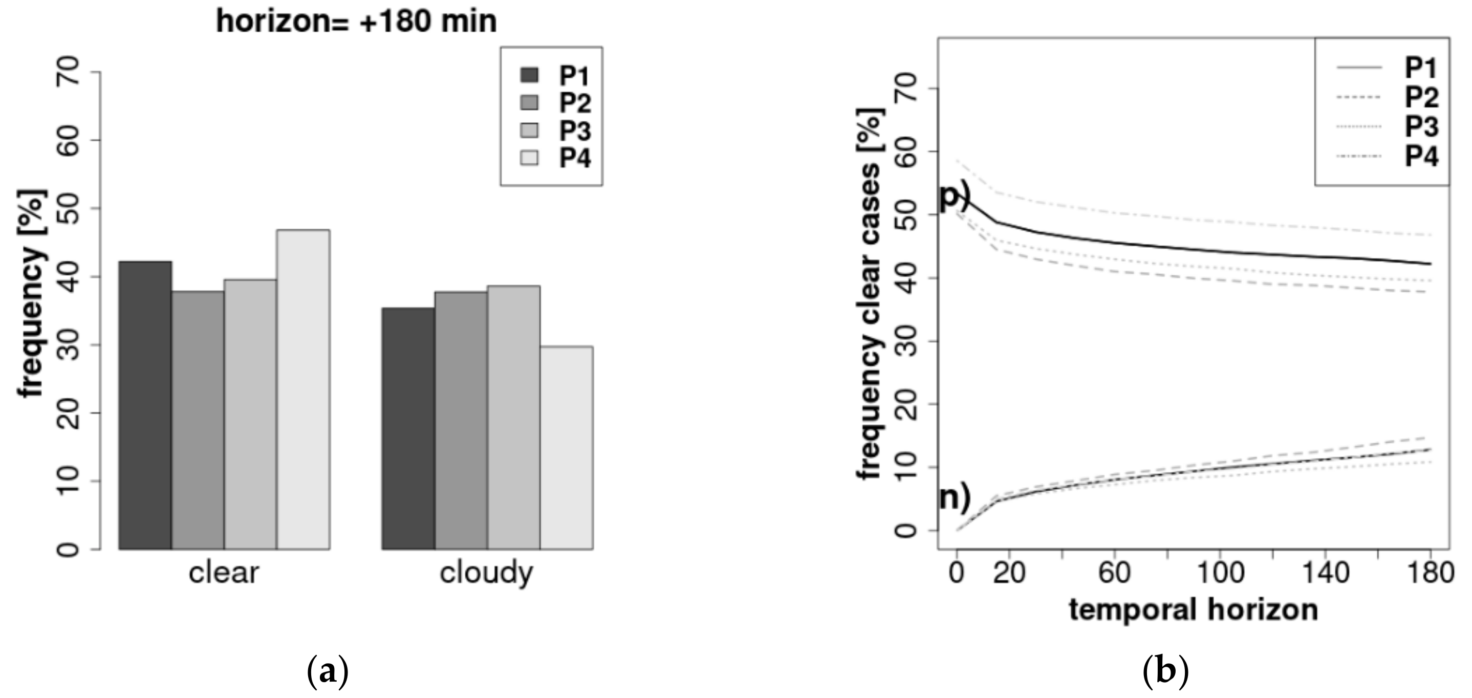
It is well known that PV power production varies accordingly to irradiance variations, that may occur at different time scales—from seconds until decades—and the frequency of variations relies with the climate of the region where the PV plant is installed. For this reason, the same power forecasting method can achieve different accuracy levels, depending on the climatic conditions of the region where the plant is placed. In order to look into this matter, the developed PV power forecasting methods have been applied to four PV plants, located in various Italian regions, characterized by heterogeneous climate and orography. Italy, in fact, is a small country, but with a large variability in orography. Approximatively 35% of the territory is mountainous, 40% hilly and is almost completely surrounded by the sea. This results in a large variety of microclimates and frequent variations in weather conditions. For this reason, the results have been specifically analyzed in view of the distribution of the cloudiness in correspondence of each site.

The work also aims at looking into several aspects of the forecasting performance, by means of the analysis of a wide range of error indexes, in order to provide an overall view on the prediction system in various climatic conditions.

Main contributions of this paper are summarized as follows:

• A new multi-time frames solar power forecasting method is developed by combining a ST and a VST forecasting system.
• The ST is based on a multimodel approach applied to the AnEn technique.
• The output of the ST is used as explanatory variable of ARIMAX in the VST.
• A smart power persistence forecast is introduced.
• The performances are evaluated in view of the cloudiness variability of the sites, exploiting meteorological satellite data.

The paper is organized as follows: in Section 2 a description of the plants on which the methods have been tested together with the data used in this work is given (Section 2.1 and Section 2.2 respectively). In the same section, the implemented methods and the performance metrics are discussed (Section 2.3 and Section 2.4 respectively). In Section 3 the results are analyzed, while Section 4 is devoted to a discussion on the results. The specific performance analysis in view of the cloudiness variation of the sites is reported in Appendix A.

2. Materials and Methods

2.1. Power Output

The PV power forecast for multiple time frames has been tested on four Italian small-scale grid-connected PV plants. The first plant, named P1, is located in the South of Italy, on flat terrain. Two other plants, named P2 and P3, are installed in central Italy. P2 is characterized by an installation in complex terrain, at an altitude of 900 m, whereas the last plant—P4—is placed in the North of Italy, in Ligury, a few kilometres from the sea. It is situated in a valley surrounded by relative high mountain ranges. Because of its position, it is characterized by peculiar climatic conditions. The siting of the plants, with the orography, is presented in Figure 1.

The plants differ each other for size, typology of panels and orientation. In particular, P4 is oriented to Est.

The main characteristics of the installations are summarized in

Table 1. Main characteristics of the PV plants. Note that P4 has an exposition of 17° East.

Plant	Nominal Power (kWp)	Type	Orientation	Inclination
P1	14.76	mono c-Si	180°	30°
P2	49.68	mono c-Si	180°	30°
P3	19.8	Polycrystalline	180°	30°
P4	14.88	mono c-Si	163°	30°

.

15-min interval power data from 2016 to the end of 2019 from the four plants have been collected in order to develop and test the ST and the VST. In particular, the ST has been trained during the period July 2016–October 2018, while the multi-time frame system has been performed and tested during the period from November 2018 until November 2019. The test, performed over a complete year, enabled it to evaluate the performance of the method in different seasonal conditions. The dataset used for the test contains only day-time data, with a size of around 15,000 samples, depending on the availability of the power measurements during the year.

In Figure 2 the temporal evolution of the PV production and the corresponding Global Horizontal Irradiation (GHI), for the four plants, from July 2016 to November 2019 is shown.

By comparing the temporal evolution of the production (graphs b, d, f, and h in Figure 2) with the progress of the GHI (graphs a, c, e, and g in the same figure), it is possible to note the strong relationship among these fields for all the plants except for plant P1 which underwent a revamp in 2019, so that its production in 2019 was higher than in previous years. On the contrary, plant P3 suffered inverter failure in May 2019, resulting in a reduction in production capacity.

It is also possible to notice the considerable variability in both inter- and intra-annual radiation and production. This simple comparison supplies a clear picture of the operational conditions that can occur and points out that a real-time forecasting method must try to quickly adapt to the always possible changes in the system characteristics as well as irradiance variations.

2.2. Meteorological Data

Different sources of meteorological information have been used in this study. Weather data have been used in part as predictors of the power forecasting methods and in part to evaluate the performance variations in function of the climatic properties of each site, as described in Section 3 and in Appendix A.

2.2.1. NWP Forecast

The forecast of the weather variables affecting PV production, used as input of the short-term PV forecast, has been derived from two different numerical weather prediction models: the Weather Research and Forecasting Model (WRF) [42] and the Regional Atmospheric Modeling System (RAMS) [43].

They are local area models, driven with initial and boundary conditions supplied by a global area model. The run of each local area model has been performed using two different global NWP models that provided the initial and boundary conditions. The used global NWP models are the Integrated Forecast System (IFS), developed by the European Centre for Medium Range Weather Forecasts, UK (ECMWF), and the Global Forecast System (GFS), developed by the National Oceanic and Atmospheric Administration, USA (NOAA).

In this study, both WRF and RAMS have been run once a day, with start at 12 UTC. Each run has supplied the weather forecast for the following three days, with a spatial resolution of 4 km and a time resolution of 1 h over a domain covering the Italian territory. For each PV plant, the weather forecast on the nearest NWP model point has been used and a temporal interpolation has been performed in order to obtain a fifteen-minute weather forecast up to three days ahead.

Because of the use of the two local area models and the two drivers, each weather variable has been forecasted by four different model chains, hereinafter referred to:

• WGN = WRF + GFS
• WES = WRF + IFS
• RGN = RAMS + GFS
• RES = RAMS + IFS

A scheme, to describe the four NWP chains, is reported in Figure 3.

The weather variables used to perform the short-term forecast are:

• Global Horizontal Irradiation (GHI)
• Diffuse Horizontal Irradiation (DHI)
• Direct Normal Irradiation (DNI)
• Wind speed at 10 m (WS)
• Relative Humidity (RHU)
• Panel Temperature (TPAN)
• Precipitable Water Content (PWC)

Some considerations about the choice of the weather input for the ST are reported in Section 2.3.1.

2.2.2. Satellite Data

Many authors agree on the benefit of using meteorological satellite information for the intra-day horizon of the PV power forecast, such as Barbieri et al. [12], Carriere et al. [40], Kühnert et al. [44]. The recent work of Yu [45] showed the performance improvement for a PV power generation prediction system based on the Eidetic three-dimensional (E3D)-long short-term memory (LSTM)-E3D-LSTM-model, when the future cloud amount from satellite data is included in the model with respect to the same model without cloud information inferred from satellite.

In this study also, for the VST PV power forecast, the information on the state of the sky in terms of cloudiness has been inferred from the geostationary satellite Meteosat Second Generation (MSG), operated by the European Organization for the Exploitation of Meteorological Satellites (EUMETSAT) [46]. The Spinning Enhanced Visible and Infrared Imager (SEVIRI), on board the MSG, provides data on 12 spectral channels, observing the Earth with a repeat cycle of 15 min and a spatial resolution of 3 km at the sub-satellite point for 11 channels, while a finer resolution of 1 km is available for the high-resolution visible channel, covering the range of wavelength 0.6–0.9 µm. Through the package CloudType of the free software SAFGEO issued by the European Organization of Meteorological Satellites (EUMETSAT), represented by the Agencia Estatal De Meteorologia (AEMET), Madrid, Spain [47], the satellite images in the different channels have been analyzed and elaborated in order to classify each satellite pixel according to a particular type of cloudiness.

With this software, the nearest pixel to each PV plant has been classified, every fifteen minutes, according to the list presented in

Table 2. Cloud type classification of the SAFGEO software.

Class	Cloud Type Category
1	Cloud-free land
2	Cloud-free sea
3	Snow over land
4	Sea ice
5	Very low and cumuliform clouds
6	Very low and stratiform clouds
7	Low and cumuliform clouds
8	Low and stratiform clouds
9	Medium and cumuliform clouds
10	Medium and stratiform clouds
11	High opaque and cumuliform clouds
12	High opaque and stratiform clouds
13	Very high opaque and cumuliform clouds
14	Very high opaque and stratiform clouds
15	High semi-transparent thin clouds
16	High semi-transparent meanly thick clouds
17	High semi-transparent thick clouds
18	High semi-transparent above low or medium clouds
19	Fractional clouds (sub-pixel water clouds)

.

On the basis of the cloudiness and considering the relative position of the sun with respect to the satellite pixel at each time, the authors have derived an estimate of the GHI on the ground by means of a polynomial regression [48].

GHI has been derived from the cloud type and the Solar Zenith Angle (SZA) by means of the general formulation:

$$GHI\mathrm{Sat}={{\displaystyle \sum }}_{i=1}^3{a}_{i,CT}\ast {(\mathit{cos}\left(SZA\right))}^i$$

(1)

where the coefficients $a_{i,CT}$ are cloud type dependent.

The estimation of the GHI, obtained from satellite data, has provided an input of the VST model—hereinafter referred to GHI-Sat.

In practice, for each time-horizon of the VST range, the predictor concerning GHI has been calculated according to these steps:

1.

Attribution of the cloud type on the closest satellite pixel to the plant, using the latest available satellite data.

2.

Calculation of the SZA on the site for the next horizons (+15 min, +30 min etc.)

Application of the abovementioned polynomial regression (Equation (1)) to derive the GHI in the future, assuming a persistence of the cloudiness and using the SZA at the time the forecast applies. In presence of cloudiness with rapid variations both in shape and in physical properties, the accuracy of this GHI forecast can rapidly worsen with increasing horizons, but it supplies a valuable update of the NWP forecast of the GHI by the way. It has been in fact proved by Dambreville et al. [49] that satellite-based methods outperform NWP forecast in the range of horizons +30 min +6 h with regard to GHI estimation.

Meteorological satellite data, besides for estimating the GHI in input at the VST model, have been used to characterize the weather conditions in correspondence of the installations in terms of cloudiness. By analyzing the cloudiness distributions on each plant, some considerations on the influence of weather conditions on the performance of the methods have arisen, as discussed both in Section 3 and in Appendix A.

2.3. PV Power Forecasting Methods

The multistep PV power forecasting has been achieved through two consecutive steps:

1.

Carrying out the short-term PV power forecast for the next three days with a time resolution of fifteen minutes. This forecast was performed once a day, at 12 UTC.

2.

Carrying out the very-short-term power forecast every fifteen minutes, with validity up to three hours ahead.

A scheme of the process is reported in Figure 4:

2.3.1. Short Term Forecast

The short-term forecast has been performed with a temporal horizon of three days and a time resolution of fifteen minutes. It has been based on a multimodel approach, both in relation to the weather information and with respect to the statistical technique used to convert weather information in power forecast.

The final ST prediction has been obtained by first evaluating a set of single power forecasts based on the Analog Ensemble (AnEn) method introduced by Delle Monache et al. [50] and then applying an optimization procedure, according to the approaches proposed by Kioutsioukis et al. [51] and applied by Collino et al. [52].

The AnEn method looks for a set of past events when some prescribed variables had assumed values close to those expected in the current forecast. For this study, the variables used to find similar past events were the weather variables affecting PV power production, derived from the NWP models mentioned in Section 2.2.1. The power measurements recorded in the past in correspondence of those “analogues” events have been used to create a probability distribution function of forecasted power. It is worth pointing out that the weather forecasts are only used to identify past moments for which the particular NWP model had provided a forecast similar to the current one, without actually entering into the production calculation process. The assumption is that the behavior of the NWP model does not change over time (the software is the same with the same parametrizations). By using a past period with power measurements and corresponding NWP forecast, it is safe to assume that, by comparing the current weather forecast with many past ones, it is possible to identify past power measurements that are presumably close to the ones we are going to predict. This condition is valid if the past period for finding similar events is long enough to ensure that most of the typical local weather conditions have occurred in the site where the plant is installed. In our case, a period of 29 months, from July 2016 to November 2018, has been used to identify the similar events.

From this set of past productions, it is possible to build a pdf from which to calculate average and median. The pdf is made up by managing an ensemble of past measurements, which naturally carry all the characteristics of the solar installation. In this way, some features, e.g., tilt, exposition or presence of azimuthal tracker and so on, are automatically taken into account. It is important to note that, because this pdf may not be normal, average and median may differ greatly from each other.

In this study, the predictors adopted to find the similar past events were: the astronomical solar angles, i.e., solar elevation (ELEV) and azimuth (AZI), the three solar irradiation components (GHI, DHI and DNI), the panel temperature (TPAN), the total precipitable water content within the vertical column of atmosphere above the solar plant (PWC), the relative humidity at 2 m (RHU), and the wind speed at 10 m above the ground (WS).

The PV panel temperature was evaluated by means of the formulation reported in Equation (2), derived by Skoplaki et al. [53]:

$$TPAN=T_{2m}+\frac{NOCT-20°}{800}GTI$$

(2)

where $T_{2m}$ is the air temperature at 2 m above ground, GTI the global tilted irradiation, and NOCT the Nominal Operating Cell Temperature proper to the module type, defined as the temperature reached by open circuited cells in a module under standard conditions.

A preliminary analysis to identify suitable variables to be used to assess similarities was carried out by analyzing the correlograms between possible features and power measurements. This analysis was performed for all PV plants, using power measurements and corresponding weather forecasts obtained from the four NWP models for one year (November 2018 to October 2019).

Figure 5a shows the correlograms, relative to plant P1, among the AnEn input variables, predicted by the NWP WES, and the production, while Figure 5b shows the highest or lowest relationships between POWER and the variables predicted by the four NWP for all the PV plants. In addition to the numeric values, the correlogram underlines stronger relationships by means of greater dimension of the circles and with warm colors, while small circles with cool colors represent lower correlation.

It is interesting to observe the high correlation of the panel temperature with power, and the very low relevance of precipitable water content and wind speed. Since TEMP is less relevant than TPAN, air temperature was not used as a predictor, also to avoid redundancies and over-weighting the temperature contribution in the selection of the similar cases. Regarding PWC, it is important to be aware that the cloud cover used in the radiative transfer models within the NWP models could be significantly different from the one obtained as output of the NWP, because it is generally derived from independent schemes (radiative transfer models usually require knowledge of the cloud optical depth provided by NWP’s microphysics, whilst most cloud cover schemes are based on columnar RHU functions). For this reason, PWC was also included in the list of AnEn features. Wind intensity was also considered, despite its low relationship with power, with a view to creating a generalized model and taking into account that wind has a significant rule in heat dissipation and could affect module efficiency, especially in locations with variability in wind regimes and for outdoor installations.

All these weather variables have been provided by the regional models mentioned in Section 2.2.1. The two regional models (WRF and RAMS), driven by the initial and boundary conditions supplied by two different global NWP (IFS and GFS), have made it possible to obtain four different NWP configuration, named RES, RGN, WES, WGN, as shown in Figure 4. Since the outputs of these models have an hourly time step to save calculation resources, the weather time series have been linearly interpolated with a resolution of 15 min, in accordance with the time resolution of the power measurements.

As mentioned above, AnEn looks for similar past events by minimizing the distance between the current set of predictors and the past ones. The metric adopted for evaluating the distance between the current vector of predictors and the past forecasts is the one reported in Equation (3), named absolute distance in the following:

$$d_{Abs}\left(t,t^{\prime }\right)={\displaystyle \sum }_{v=1}^{N_v}\frac{w_v}{{\sigma }_v}\left|F_{v,t}-A_{v,t^{\prime }}\right|$$

(3)

where v represents each variable of the set of $N_v$ predictors, $F_{v,t}$ the v-th component of the array of the current forecast for the forecast horizon t, and $A_{v,t^{\prime }}$ the v-th component of the past forecasts relative to the same temporal horizon of $F_{v,t}$. Each variable used to evaluate the distance has been previously normalized using the standard variation ${\sigma }_v$ of each variable inside the training period considered. For this study, the training period ran from July 2016 to November 2018, and the test period from November 2018 to November 2019. The training and test periods are chosen large enough to avoid monthly calendar effect, whilst yearly effects may occur due to climatological anomalies. According to the formulation reported in Equation (3), it is also possible to set different weights for each variable through $w_v$. Compared to the AnEn introduced by Delle Monache et al. [50], the AnEn implemented in this study has some different features, such as the fact that the metric compares only the predictors at the same temporal horizons, and the absolute distance is adopted instead of the Euclidean one. Furthermore, in the selection of similar past events a constraint has been imposed on the astronomical angles, considering only the events for which the past and the current zenith angle differed for less than 10 degrees, and the azimuths for less than 20 degrees, in order to guarantee similar solar positions.

For each plant, at each NWP forecasting run, different AnEn setups have been performed, by varying the configuration of the AnEn according to the following criteria, summarized in

Table 3. List of the AnEn configurations.

Configuration Parameters				NWPs
Config	${\mathit{N}}_{\mathit{p}\mathit{d}\mathit{f}}$	${\mathit{w}}_{\mathit{v}}$	PCA	RES (RAMS + IFS)	RGN (RAMS + GFS)	WES (WRF + IFS)	WGN (WRF + GFS)	MM
WI	21	yes	no	IREWI	IRGWI	IWEWI	IWGWI	IMMWI
WJ	31	yes	no	IREWJ	IRGWJ	IWEWJ	IWGWJ	IMMWJ
WM	21	no	no	IREWM	IRGWM	IWEWM	IWGWM	IMMWM
WN	31	no	no	IREWN	IRGWN	IWEWN	IWGWN	IMMWN
PM	21	no	yes	IREPM	IRGPM	IWEPM	IWGPM	IMMPM
PN	31	no	yes	IREPN	IRGPN	IWEPN	IWGPN	IMMPN

:

• The inputs used by the AnEn:

There were used weather forecasts provided by a single NWP model of the four described in Section 2.2.1 (RES, RGN, WES, WGN), or by all of them simultaneously (MM). In the latter case the meteorological input was made of 28 weather variables (the 7 meteorological variables listed above and provided by the 4 NWP models).

• The application of a pre-processing on the predictors by means of:

Principal Component Analysis (PCA). Instead of using the forecasted weather variables, the distance was calculated using the N_PCA principal components selected on the basis of the explanation of the 95% of the variance. PCA was only used to create additional ensemble members, again based on Analog Ensemble. Basically, the aim was to reduce the cardinality of the input set, especially when all four NWP models, i.e., 28 weather variables, were used, to avoid curse of dimensionality problems.

• The number of elements of the pdf:

The metric (Equation (3)) allows to identify the N_pdf past events more similar to the current one. The number N_pdf is another free parameter, usually set to the square root of the length of the training dataset. Beside the value suggested by the thumb rule (N_pdf = 21), the case N_pdf = 31 was also used.

• Application of some weights to the predictors:

Some configurations (WI and WJ) considered variable-dependent weights, obtained after a sensitivity study, whilst in the other cases each variable was normalised only for its standard deviation.

According to the presented criteria, by applying the Equation (3) it has been possible to select an ensemble of past N_pdf power measurements with which to build different probability distribution functions of the expected production. From these pdfs, the average, the median and the major percentiles have been computed for each of the configurations summarized in Table 3.

Once the configured forecasts have been performed, an optimization procedure has been applied to their ensemble E, based on the minimization of the following error, described by Kioutsioukis [51]:

$$MSE\left(\overline{f}\right)={\overline{bias}}^2+\frac{1}{M}\overline{varE}+\left(1-\frac{1}{M}\right)\overline{covE}$$

(4)

which states that the mean squared error (MSE) of an ensemble (E) of single forecasts is made up of three contributes: bias, variance and covariance of the ensemble composed of M members. In order to optimize the ensemble, both the mean and the median of each pdf have been used in Equation (4), for a total of 60 members. Since the members of the ensemble were correlated to each other, the optimized forecast (solution of Equation (4)) has been written as a weighted average of the M members:

$$\overline{f}={\displaystyle \sum }_{k=1}^M{a}_k{f}_k\stackrel{\scriptscriptstyle\mathrm{def}}{=}\frac{{\underset{\_}{K}}^{-1}\underset{\_}{u}}{({\underset{\_}{K}}^{-1}\underset{\_}{u},\underset{\_}{u})}·f$$

(5)

where $\overline{f}$ is the ensemble average, $\underset{\_}{K}$ the ensemble’s correlation matrix, $f_k$ the k-th member of the ensemble, and $\underset{\_}{u}$ is a vector of ones of length M. Following this approach, the weights $a_k$ may not be definite positive, allowing some sort of compensation between different ensemble members, i.e. between different AnEn configurations and/or NWP outputs (positive weights are obtained only if the ensemble members are uncorrelated).

The advantages of applying the ensemble optimization method are discussed in Section 3.

2.3.2. Very Short-Term Forecast

The forecast for the following three hours, with a time resolution of fifteen minutes has been based on an Auto-Regressive Integrated Moving Average Model with eXogenous input (ARIMAX). ARIMAX is a multivariate version of the time series method ARIMA and its use in PV power forecasting has been explored by only a few authors so far, such as Zhou et al. [13], Bacher et al. [17], Perez-Mora et al. [18]. ARIMA method is a generalization of ARMA modelling with the advantage of handling nonstationary time series. It was introduced by Box and Jenkins [54]. ARIMA is made up of three elements: autoregression (AR), integration (I) and moving average (MA). It is characterized by three parameters (p,d,q), where p is the number of time lags of the autoregressive model, d is the degree of differencing and q is the order of the moving-average model.

In the past only observed or predicted GHI, air temperature, or PV panel temperature were considered as input of ARIMAX devoted to forecast PV power. Yang in [55] claimed the lack of weather information on time series models developed so far. In this study an innovative autoregressive method has been carried out, focusing on the use of new exogenous inputs and exploring the usefulness of introducing irradiance data derived from satellite and power forecasts obtained from independent methods as predictors.

The exogenous variables selected as input of the very-short-term forecasting are:

• GHI from satellite data (GHI-Sat)
• GHI from satellite data (GHI-Sat)
  Smart Power Persistence (SP)
• Short-Term PV power Forecasting (ST)

The predictor GHI-Sat has been already described in Section 2.2.2.

SP is a smart power persistence, established by considering the evolution of the solar orbit.

The persistence model (or naïve model) supposes that conditions at time t will persist into the time period $t+i$ and, for this reason, the forecast for the time $t+i$ corresponds to the power registered at the time $t: P_{t+i}=P_t$, where i represents the time lag in the future, such as minutes, hours, or even days. Solar production strongly depends on the elevation of the Sun and therefore it is possible to calculate a smart power persistence in the future, normalizing the persistence with the variations of the solar zenith angle on the plant and taking into account also the dependence of the extra-terrestrial radiation with time.

The formulation of the SP is reported in Equation (6):

$$P_{t+i}=P_t\frac{I_{t+i}\ast \cos {\theta }_{t+i}}{I_t\cos {\theta }_t}$$

(6)

where $P_{t+i}$ is the SP, that is the forecasted production at the step t+i, $\theta$ is the solar zenith angle and $I_t$ is the solar constant corrected with the Sun-Earth distance at each time t.

The predictor ST consists of the PV power forecast issued the day before for each time frame corresponding to the very-short-term horizons. For example, as shown in Figure 4, the nowcasting starting at 6 UTC for the next hour (7 UTC.), will use, as predictor, the ST issued the previous day at 12 UTC with time horizon +19 h, that is the power expected at 7 UTC.

The selection of the exogeneous input derives, in part, from previous studies, performed by the authors, devoted to quantify the performance of the ARIMAX model to varying input, in part analyzing the Spearman correlation between possible predictors and power measurements. Different authors, including Ahmed et al. [9] and Yang et al. [55], assert that the real challenge in PV power forecasting is the design of the model with the optimum number of inputs, avoiding irrelevant predictors, that could lead to undesirable increase of prediction variance.

The relationships among the variables have been studied for all the plants, considering one year of measurements every fifteen minutes and the corresponding possible predictors. The initial series of predictors taken into account consisted of cos(SZA), air temperature, panel temperature, GHI derived from NWP (GHI-NWP), GHI derived from satellite, SP and ST.

The relationships were found to slightly vary from place to place and according to the forecast horizon, but GHI-Sat, SP and ST were found to be the variables most related with power measurements. In Figure 6 a graphical display of the correlation matrix is presented for the plant P1. In the graph, Figure 6a is the correlogram calculated considering the exogenous input at the time horizon of 15 min, while Figure 6b refers to the 180 min forecast. The relationships among the variables are always positive.

Considering the relationships shown in Figure 6, it is possible to note that, in addition to GHI-Sat, SP and ST, also GHI-NWP and cos(SZA) present high relationships with power, but they are mutually related also with ST of which they are inputs. Therefore, in order to avoid redundancy, these two variables have not been used as predictors in the VST.

ARIMAX model has been implemented using the function auto.arima of the package forecast v8.13 of R developed by Hyndman et al. [56], applying a pre-processing to the input, in order to normalize each variable in the range 0–1. This function builds and evaluates different ARIMAX models and finally selects the best one on the basis of different possible criteria (in this study the Akaike’s Information Criterion has been used). The selection of the “optimum” ARIMAX has been performed at each run, using the last three weeks of historical power in order to create and test different possible ARIMAX and select the best one. Due to the fact that autoregressive models run very fast, for the VST it has been possible to derive every fifteen minutes an updated model, adapted to the recent behavior of the plant.

2.4. Performance Metrics

The developed models have been evaluated considering a wide range of performance metrics: normalized Mean Bias Error (nMBE), normalized Mean Absolute Error (nMAE), normalized Root Mean Square Error (nRMSE), Forecast Skill with respect to MAE (FSMAE), Forecast Skill with respect to RMSE (FSRMSE).

The normalization of the errors has been performed with respect to the maximum value of measured power. It is common that the PV plant output does not achieve the nominal power and therefore the normalization with respect to the maximum registered, instead of the nominal power, is more useful in order to quantify the errors in operational conditions.

In Equations (7)–(11) the definitions of the error metrics are reported, considering that W^fore, W^obse, W^Mobse,, N, mod, ref represent the forecasted power at each time point, the corresponding measured power, the maximum observed power, the sample size, the forecasting model and the reference model respectively.

$$nMBE=\frac{\frac{1}{N}{{\displaystyle \sum }}_{k=1}^N\left(W_k^{fore}-W_k^{obse}\right)}{W^{Mobse}}\times 100$$

(7)

$$nMAE=\frac{\frac{1}{N}{{\displaystyle \sum }}_{k=1}^N\left|W_k^{fore}-W_k^{obse} \right|}{W^{Mobse}}\times 100$$

(8)

$$nRMSE=\left(\sqrt{\frac{1}{N}{\displaystyle \sum }_{k=1}^N{\left(W_k^{fore}-W_k^{obse}\right)}^2}\right)\times \frac{100}{W^{Mobse}}$$

(9)

$$FSMAE=1-\frac{nMA{E}_{mod}}{nMA{E}_{ref}}\times 100$$

(10)

$$FSRMSE=1-\frac{nRMS{E}_{mod}}{nRMS{E}_{ref}}\times 100$$

(11)

Regarding error metrics, the authors have decided to evaluate the forecasting skill, both with respect to nMAE and nRMSE. At present, in fact, there is no consensus about the preference for MAE or RMSE in determining the forecasting performance (see Cort et al. [57], Botchkarev et al. [58], Choi et al. [59]). It is important to be aware that each error metric describes a particular aspect of the model error characteristics. For this reason, it is useful to consider different types of metrics, in order to better describe the model performance according to various aspects, such as systematic over/under estimation, magnitude of the errors in absolute and quantification of large errors.

The errors have been calculated considering only day-time data and for each time horizon, to compare the usefulness of the methods varying the forecasting horizon.

The reference model used to calculate skill scores both for the ST and the VST forecasting is the smart power persistence, described in Section 2.3.2.

For a better understanding of the influence of ST errors to VST forecasts, the Mean Absolute Error $MAE=\frac{1}{N}{\sum }_{k=1}^N\left(W_k^{fore}-W_k^{obse}\right)$ obtained using ST and VST forecasts have been analyzed in order to calculate the real-time performance of the ST and VST during the whole test period.

In practice, we have considered different prediction horizons of the VST, from 60 min up to 150 min, although the comparison is mostly useful for the 60- and 90-min horizons. For each plant, for evaluating the real-time errors for each day $d$ belonging to the test period, the starting times $t_{start}\in \left[t_{sunrise}+{\rm K},t_{sunset}-{\rm K}\right]$ ($t_{sunrise}$ and $t_{sunset}$ are the time of sunrise and sunset respectively) and different forecast horizons ${\rm K}\in \left\{60,90,120,150\right\}$ have been considered. The forecasted ST and VST power production can be formally expressed as in Equations (12) and (13) respectively:

$$P^{ST}\left(d-1;12+t_{start};f_m\right)$$

(12)

$$P^{VST}\left(d;t_{start};f_m\right)$$

(13)

where the ST run starting at 12 UTC of the day before the current one is signed as $(d-1$), and the forecasts $f_m\in F_K$, $F_K=\left\{15, 30,\dots ,K\right\}$ with steps of 15 min. According to the same notation, the measured power production of the plant, relative to the hour $\left(t_{start}+f_m\right)$ of the day $d$, is $P^{meas}\left(d;t_{start}+f_m\right)$. The real-time forecast error is evaluated at each starting time by averaging the absolute errors for all the forecasts belonging to the set $F_K$. In particular, Equation (14) relates to the ST forecast and Equation (15) to the VST forecast.

$${\mathsf{{\rm E}}}_K^{ST}(d;t_{start})=\frac{1}{\left(K/15\right)}{\displaystyle \sum }_{f_m\in F_K}\left|P^{ST}\left(d-1;12+t_{start};f_m\right)-P^{meas}\left(d;t_{start}+f_m\right)\right|$$

(14)

$${\mathsf{{\rm E}}}_K^{VST}(d;t_{start})=\frac{1}{\left(K/15\right)}{\displaystyle \sum }_{f_m\in F_K}\left|P^{VST}\left(d;t_{start};f_m\right)-P^{meas}\left(d;t_{start}+f_m\right)\right|$$

(15)

The range of ${\mathsf{{\rm E}}}_K^{ST}$ is the interval $\left[0, {\mathsf{\Delta }}_K\right]$, which is divided into $n_{\delta }$ (set equal to 300 in this study) subintervals of equal width.

To guarantee the synchronization of the errors provided by ST and VST, data are partitioned in a set of disjoint and adjacent sets $\left\{A_r\right\}$ defined as reported in Equation (16):

$$A_r=\left\{\left(d;t_{start}\right) |\frac{\left(r-1\right){\mathsf{\Delta }}_K}{n_{\delta }}\le {\mathsf{{\rm E}}}_K^{ST}<\frac{r{\mathsf{\Delta }}_K}{n_{\delta }} \wedge r\in \left[1,n_{\delta }\right]\right\}$$

(16)

The partitioning is performed with respect to ST errors belonging to the whole test period. This means that the set $A_{\widehat{r}}$ contains the time labels of the events for which the ST errors lie in an interval of width ${\mathsf{\Delta }}_K/n_{\delta }$ starting at $(\widehat{r}-1){\mathsf{\Delta }}_K/n_{\delta }$. Naming ${\epsilon }_r^{ST}$ the centre of this interval, the total run-time error (expressed in power units) for each subinterval is defined as:

$$Q^{ST}= {\displaystyle \sum }_{\left(d;t_{start}\right)\in A_r}{\mathsf{{\rm E}}}_K^{ST}\left(d;t_{start}\right); Q^{VST}= {\displaystyle \sum }_{\left(d;t_{start}\right)\in A_r}{\mathsf{{\rm E}}}_K^{VST}\left(d;t_{start}\right)$$

(17)

and the corresponding cumulative quantities as:

$$C^{ST}\left({\epsilon }_r^{ST}\right)= {\displaystyle \sum }_{k=1}^r{Q}_k^{ST}\left({\epsilon }_k^{ST}\right); C^{VST}\left({\epsilon }_r^{ST}\right)= {\displaystyle \sum }_{k=1}^r{Q}_k^{VST}\left({\epsilon }_k^{ST}\right)$$

(18)

The analysis of the errors is discussed in Section 3.

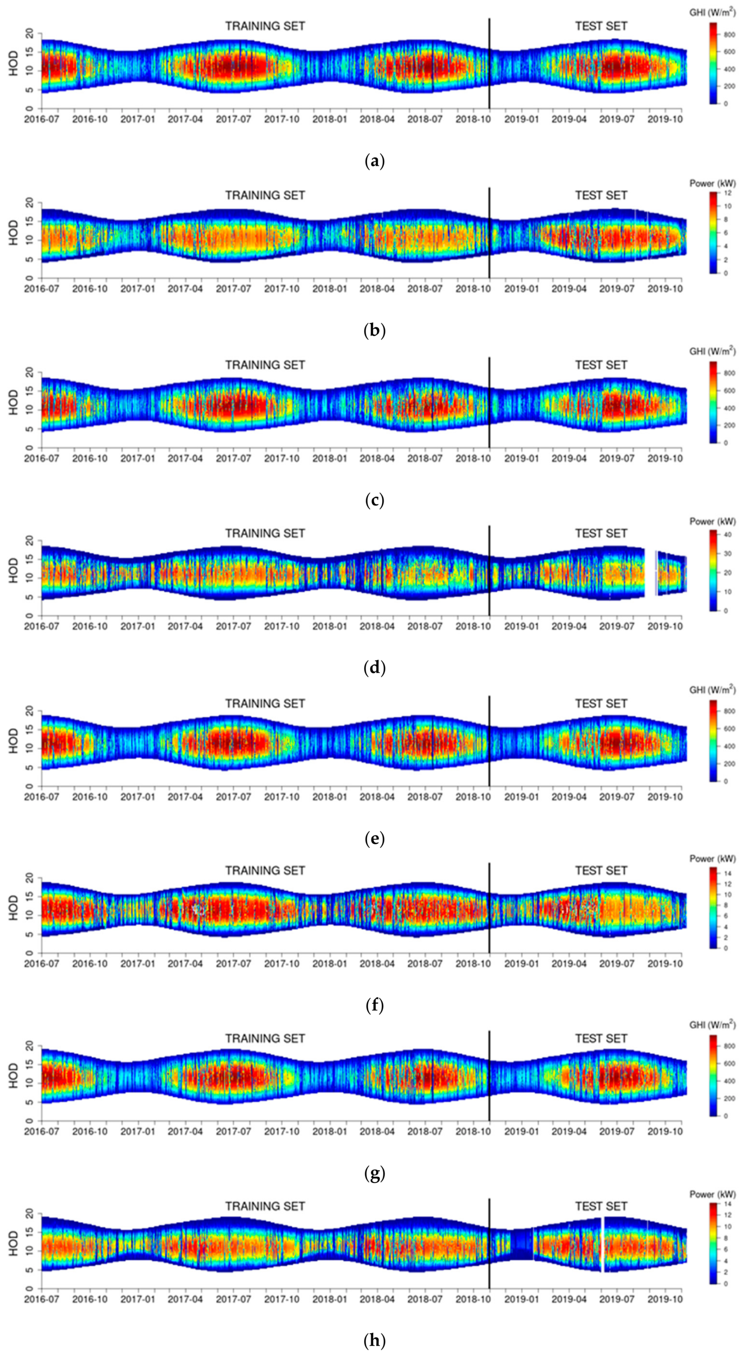
3. Results

In this work, both the ST and VST forecasting models have been applied to forecast the PV production at four different Italian sites, during the period November 2018–November 2019. The PV plants and the used dataset have been described in Section 2.1, while the analyzed error metrics have been presented in Section 2.4. All the tested methods have been compared with the smart power persistence, introduced in Equation (6) and used as reference.

Firstly, the general ability of the ST in predicting PV power, up to three days ahead has been considered.

As described in Section 2.3.1, the optimized short-term forecast has been obtained by solving Equation (5), using 60 member ensembles made up of the average and medians provided by the AnEn pdfs.

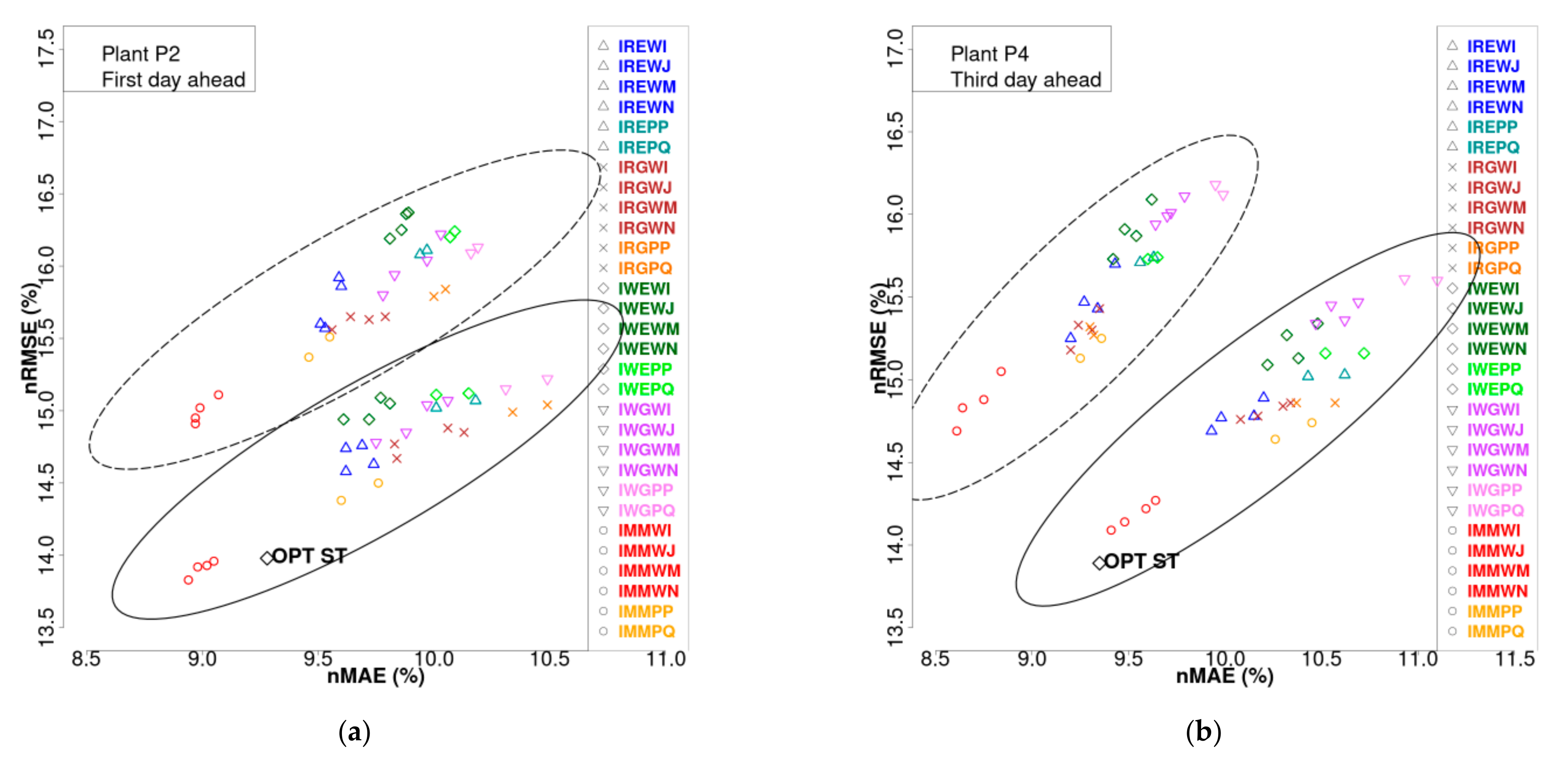
In Figure 7 the nRMSE vs. nMAE for each ensemble member is shown for the plants P2 and P4 and for the first and third forecasting day, respectively. The most relevant considerations that can be made are that medians get larger errors than averages, the MM forecasts—corresponding to the red circles and crosses at the lower ends of the ellipses—always achieve better results than any single NWP, the pre-processing with PCA generally performs worst, and finally the optimized ST always obtains smaller errors than any single AnEn forecast.

In

Table 4. nBIAS, nMAE, nRMSE, and SKILLs of the four PV plants. The values are the mean errors, in percentages, regarding the first (horizon of 12–36 h), the second (36–60 h), and the third (60–84 h) day ahead. The errors have been normalized with respect to the maximum measured value (P1_max = 12.44 kW, P2_max = 15.29 kW, P3_max = 40 kW, P4_max = 13.94 kW).

Forecast Horizon	P1				P2
	nMAE	nRMSE	FSMAE	FSRMSE	nMAE	nRMSE	FSMAE	FSRMSE
First day	9.40	13.41	27.69	36.92	9.28	13.98	33.24	37.14
Second day	9.52	13.52	34.12	41.14	9.42	14.01	38.31	41.16
Third day	9.91	13.89	30.46	38.81	9.84	14.52	36.88	39.68
Forecast Horizon	P3				P4
	nMAE	nRMSE	FSMAE	FSRMSE	nMAE	nRMSE	FSMAE	FSRMSE
First day	9.90	14.59	31.06	35.98	8.81	13.23	33.96	39.89
Second day	10.07	14.74	36.43	39.19	9.01	13.35	37.99	43.22
Third day	10.43	15.12	33.44	36.60	9.35	13.89	33.83	39.66

the normalized nMAE, nRMSE and the skills (FSMAE and FSRMSE evaluated with respect to the smart power persistence SP) of the optimized ST model are summarized. They represent the average of the errors produced in the first, second and third day of forecast during the entire verification period.

The nMAE and nRMSE of the optimized ST increase with the time horizon by about half a percentage point, moving from the first to the third day of forecasting. The better results, in terms of nMAE and nRMSE are achieved for the plant P4, probably due to its climatology, dominated by a large amount of clear sky conditions. This aspect has been investigated using satellite data in order to evaluate the general weather conditions of each site and the main findings are reported in Appendix A.

The nMAE and nRMSE of the optimized ST increase with the time horizon by about half a percentage point, moving from the first to the third day of forecasting. The better results in terms of nMAE and nRMSE are achieved for the plant P4, probably due to its climatology, dominated by a large amount of clear sky conditions. This aspect has been investigated using satellite data in order to evaluate the general weather conditions of each site and the main findings are reported in Appendix A.

Taking into account this behavior, it is interesting to consider the improvements achievable with the use of the optimized ST with respect to the smart persistence, evaluated using the observed power with lags of one, two, or three days before the forecast time for the first, second and third day of forecast respectively.

The forecast skill scores are larger than 30%, except for the FSMAE of P1 for the first day of forecast, with varying fluctuations going from the first to the third day of forecast. The nonmonotonic increase of the skills with the forecasting horizon is due to the nonconstant increase with time of the errors for the smart power persistence.

It is important to underline the ability of the optimized ST in avoiding errors of large magnitude, because the FSRMSE scores are always greater than the FSMAE ones and exceed 40% except for the plant P3, where the best score is 39.2%.

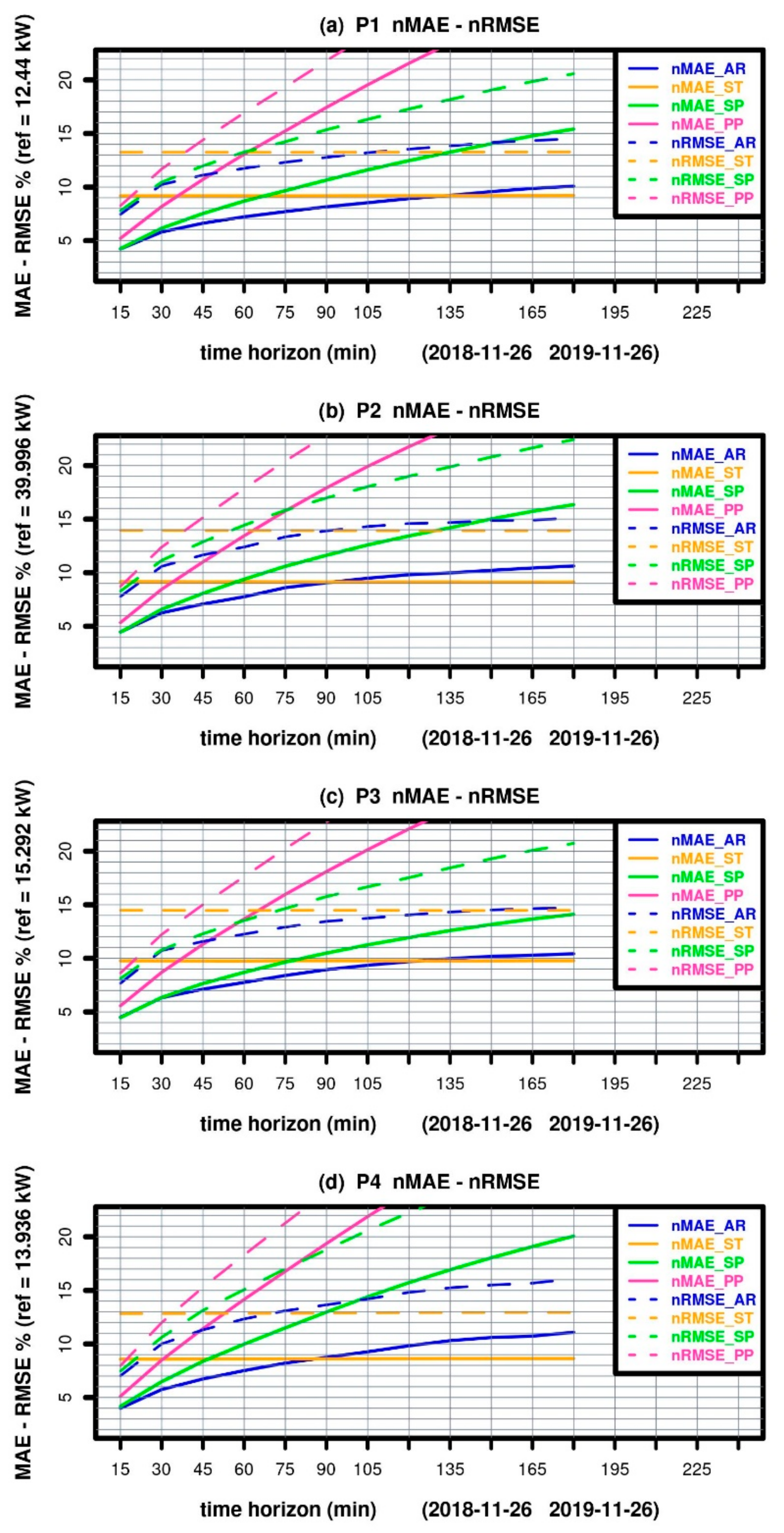
Considering the intra-day forecast, the purpose of this work was to evaluate advantages and drawbacks of different approaches, suitable for real-time applications, with varying time frames, from 15 min up to three hours ahead. In particular, having available the optimized ST forecasting for the next day, we wanted also to figure out the forecasting horizon up to which the VST outperformed the ST, in order to identify which method was preferable to use at each forecasting horizon.

Figure 8 presents the evolution of nMAE and nRMSE with the increase of the forecasting horizon, from 15 min up to the 180 forthcoming minutes for the main methods considered in this work, such as pure and smart power persistence—calculated using the last available power measurement—ARIMAX and optimized ST.

By analyzing the evolution of both nMAE and nRMSE in Figure 8, it is possible to note the outperformance of all the very-short-term forecasting methods (PP, SP, AR) with respect to the ST for the early forecasting horizons. However, after only 30 min, the ST outperforms the PP in each site.

The smart power persistence turns out to be a satisfactory PV forecasting method at least in the first hour of forecast, with nMAE ranging from about 4% to 9% with small variations depending on the plant. In the very-short forecasting range, as the time goes on, the most beneficial system, both in terms of nMAE and nRMSE, proves to be the ARIMAX. In fact, it achieves the lowest rate of errors from the beginning up to over two hours in advance for the plants P1 and P3 and up to 90 min for the plants P2 and P4. ARIMAX starts with a nMAE around 4% and a nRMSE around 7.5% and reaches values around 10.2% of nMAE and 15% of nRMSE after three hours in P1, P2 and P3 sites, while the behavior is different for P4 plant. In this case ARIMAX gains very low errors at the first horizon, with a nMAE of 3.99% and a nRMSE of 7.0%, but, after three hours, the nMAE is one percentage point larger than the one obtained in the other plants and so for nRMSE. The reason of this evolution has been investigated through analysing the climatology of the site where the plant is installed, in terms of cloudiness, as reported in Appendix A.

By analyzing the evolution of both nMAE and nRMSE in Figure 8, it is possible to note the outperformance of all the very-short-term forecasting methods (PP, SP, AR) with respect to the ST for the early forecasting horizons. However, after only 30 min, the ST outperforms the PP in each site. The smart power persistence turns out to be a satisfactory PV forecasting method at least in the first hour of forecast, with nMAE ranging from about 4% to 9% with small variations depending on the plant. In the very-short forecasting range, as the time goes on, the most beneficial system, both in terms of nMAE and nRMSE, proves to be the ARI-MAX. In fact, it achieves the lowest rate of errors from the beginning up to over two hours in advance for the plants P1 and P3 and up to 90 min for the plants P2 and P4. ARIMAX starts with a nMAE around 4% and a nRMSE around 7.5% and reaches values around 10.2% of nMAE and 15% of nRMSE after three hours in P1, P2 and P3 sites, while the behavior is different for P4 plant. In this case ARIMAX gains very low errors at the first horizon, with a nMAE of 3.99% and a nRMSE of 7.0%, but, after three hours, the nMAEis one percentage point larger than the one obtained in the other plants and so for nRMSE. The reason of this evolution has been investigated through analysing the climatology of the site where the plant is installed, in terms of cloudiness, as reported in Appendix A.

As far as concern the presence of systematic over/underestimation from the various very-short-term methods,

Table 5. Normalised BIAS and forecast skill related to MAE-FSMAE and RMSE-FSRMSE for plant P1 from 15 min up to three hours ahead.

LAG	NUM	nBIAS_AR	nBIAS_ST	nBIAS_SP	nBIAS_PP	FSMAE_AR	FSMAE_ST	FSMAE_PP	FSRMSE_AR	FSRMSE_ST	FSRMSE_PP
15	15049	0.23	−0.68	0.60	0.22	0.48	−115.88	−22.73	4.43	−69.96	−5.93
30	15035	0.14	−0.68	1.19	0.47	5.68	−49.25	−33.01	2.08	−26.84	−11.81
45	15037	0.24	−0.69	1.71	0.72	12.00	−21.99	−42.27	7.21	−10.66	−20.15
60	15036	0.30	−0.68	2.22	1.03	16.86	−5.71	−50.32	11.46	0.11	−27.66
75	15054	0.73	−0.68	2.71	1.20	20.22	5.03	−57.69	13.44	6.91	−35.88
90	15044	0.83	−0.67	3.19	1.28	23.41	13.79	−63.69	16.84	13.69	−41.99
105	15035	0.95	−0.68	3.63	1.25	26.45	20.83	−68.33	19.06	18.76	−48.26
120	15039	0.96	−0.68	4.06	1.13	28.43	26.26	−72.87	21.66	23.26	−53.44
135	15034	1.04	−0.68	4.49	0.89	30.49	30.66	−76.81	23.84	27.00	−58.10
150	15029	0.94	−0.69	4.90	0.55	31.81	34.46	−80.07	25.64	30.35	−61.84
165	15027	0.96	−0.69	5.29	0.11	33.17	37.70	−82.81	27.81	33.14	−65.62
180	15029	1.02	−0.69	5.69	-0.43	34.60	40.25	−85.78	29.47	35.48	−68.98

,

Table 6. Normalized BIAS and forecast skill related to MAE–FSMAE and RMSE–FSRMSE for plant P2 from 15 min up to three hours ahead.

LAG	NUM	nBIAS_AR	nBIAS_ST	nBIAS_SP	nBIAS_PP	FSMAE_AR	FSMAE_ST	FSMAE_PP	FSRMSE_AR	FSRMSE_ST	FSRMSE_PP
15	12916	0.20	2.28	0.36	0.00	−0.45	−105.83	−20.13	5.99	−68.43	−5.45
30	12904	0.14	2.29	0.65	−0.01	5.06	−39.09	−28.43	5.01	−25.01	−11.09
45	12912	0.31	2.29	0.88	−0.04	12.25	−13.34	−36.37	9.47	−8.18	−17.55
60	12911	0.37	2.28	1.06	−0.12	17.39	2.49	−43.21	14.08	3.38	−23.70
75	12917	0.69	2.28	1.19	−0.25	18.81	13.75	−48.70	15.69	11.99	−29.10
90	12919	0.83	2.28	1.29	−0.46	22.10	21.44	−54.07	18.09	18.00	−34.52
105	12917	0.85	2.26	1.34	−0.79	24.68	27.48	−58.20	20.63	22.80	−39.21
120	12908	0.81	2.26	1.41	−1.19	26.94	31.99	−62.05	23.24	26.75	−43.37
135	12906	0.88	2.27	1.47	−1.66	29.69	35.66	−65.42	26.15	29.98	−47.14
150	12913	0.90	2.26	1.53	−2.21	31.93	39.22	−67.36	28.56	33.11	−49.87
165	12911	0.80	2.27	1.62	−2.82	33.66	41.97	−69.71	31.18	35.74	−52.48
180	12898	0.56	2.27	1.68	−3.54	35.00	44.15	−72.27	32.58	37.94	−54.89

,

Table 7. Normalized BIAS and forecast skill related to MAE-FSMAE and RMSE-FSRMSE for plant P3 from 15 min up to three hours ahead.

LAG	NUM	nBIAS_AR	nBIAS_ST	nBIAS_SP	nBIAS_PP	FSMAE_AR	FSMAE_ST	FSMAE_PP	FSRMSE_AR	FSRMSE_ST	FSRMSE_PP
15	15979	0.05	4.00	0.13	−0.04	−0.79	−118.90	−24.87	5.40	−78.65	−6.35
30	15981	−0.03	4.00	0.17	−0.11	0.34	−53.67	−36.86	0.54	−34.19	−13.32
45	15984	−0.06	4.00	0.15	−0.24	6.83	−27.62	−47.99	5.86	−17.66	−22.10
60	15988	−0.03	3.99	0.08	−0.45	10.87	−12.13	−57.28	9.45	−6.82	−30.18
75	15957	0.12	4.01	−0.02	−0.76	12.95	−1.27	−65.48	11.82	1.15	−38.10
90	15956	0.09	4.01	−0.14	−1.14	14.75	6.82	−72.60	14.65	8.10	−44.27
105	15964	0.00	4.01	−0.27	−1.60	16.90	13.26	−78.91	17.61	13.20	−50.67
120	15961	−0.02	4.01	−0.39	−2.16	18.82	18.17	−85.04	19.83	17.44	−56.43
135	15969	−0.22	4.01	−0.55	−2.81	20.85	22.53	−89.66	22.34	21.59	−60.53
150	15963	−0.31	4.01	−0.69	−3.57	22.61	25.83	−94.58	24.76	25.05	−64.03
165	15955	−0.41	4.02	−0.80	−4.41	24.80	28.56	−98.91	27.10	27.89	−67.26
180	15960	−0.50	4.02	−0.90	−5.31	26.11	30.75	−103.50	28.96	30.15	−70.63

and

Table 8. Normalized BIAS and forecast skill related to MAE–FSMAE and RMSE–FSRMSE for plant P4 from 15 min up to three hours ahead.

LAG	NUM	nBIAS_AR	nBIAS_ST	nBIAS_SP	nBIAS_PP	FSMAE_AR	FSMAE_ST	FSMAE_PP	FSRMSE_AR	FSRMSE_ST	FSRMSE_PP
15	11339	0.20	−0.65	0.60	−0.01	4.21	−105.53	−22.64	5.80	−71.91	−6.82
30	11334	0.08	−0.65	1.11	−0.07	11.32	−32.43	−31.02	5.79	−20.84	−12.90
45	11328	0.21	−0.65	1.60	−0.15	19.61	−2.57	−36.40	13.83	2.16	−16.31
60	11322	0.25	−0.64	2.03	−0.28	24.69	13.83	−41.88	18.14	14.67	−21.52
75	11324	0.35	−0.62	2.44	−0.47	28.55	25.25	−45.93	22.98	24.39	−25.16
90	11318	0.44	−0.62	2.84	−0.72	32.54	33.68	−49.28	27.40	31.49	−28.68
105	11313	0.42	−0.60	3.25	−1.05	35.63	40.16	−52.03	31.05	37.39	−31.21
120	11311	0.26	−0.59	3.65	−1.46	37.49	45.13	−54.50	33.40	41.95	−33.63
135	11303	0.15	−0.59	3.99	−1.98	39.08	48.98	−56.92	36.02	45.75	−35.49
150	11305	0.06	−0.59	4.35	−2.57	41.24	52.14	−59.02	38.64	48.79	−37.33
165	11307	0.08	−0.59	4.69	−3.25	43.80	54.75	−60.63	41.28	51.52	−38.39
180	11306	−0.10	−0.58	5.05	−3.99	44.73	56.95	−62.21	42.66	53.89	−39.36

present the relative nBIAS for each plant in function of the time horizon. PP shows a general underestimation, with increasing values as the forecasting horizon grows, except for the plant P1, where a slight overestimation is experienced. Instead, SP shows different behaviors at the various locations. An important overestimation, with growing values as the lead-time increases, is registered for the plants P1 and P4, while lower values are obtained for P2. On the contrary, at the P3 site, the nBIAS is very low, with a slight underestimation for lead-times beyond one hour. The ST has positive nBIAS for plants P2 and P3, while there is a slight underestimation for P1 and P4.

In addition to systematic errors, both producers and system operators are interested in assessing how much a method is beneficial with respect to another one, in absolute terms, and to quantify the presence or absence of large errors. In order to make this comparison easier, the skill of the forecast with respect to the SP system, used as benchmark, has been calculated according to the Equations (10) and (11). It is important to note that, despite its simplicity, SP is a powerful prediction system. Its reliability can be verified by comparing its performance with respect to the performance of the PP, analyzing in details the progress of the errors in Figure 8. Already at the first lead time (+15 min), SP gets a nMAE one percentage point lower than PP and the gap widens more and more with increasing forecasting horizons. The authors have also implemented an ARIMA forecasting tool for each plant. ARIMA is often used as baseline for the VST, but it got worst performances with respect to SP, therefore the authors have set to using SP as a robust baseline to deal with. Table 5, Table 6, Table 7 and Table 8 report the FSMAE and the FSRMSE for each plant according to the lead-time.

As far as FSMAE concerns, with ARIMAX, the skill is always positive, except for the plants P2 and P3, where it is slightly negative at the first horizon, confirming the validity of the SP as a useful forecasting method for the first horizons.

The FSMAE of ARIMAX grows as the time goes on. The greatest benefit is registered for plant P4, with a value of 44.7% at the 180 min time horizon. This result must be nevertheless compared with ST. Even if FSMAE of ST is negative, in general, during the first hour, it exceeds ARIMAX beyond 120 min for the plants P1 and P3 and over 75 min for sites P2 and P4. By considering the FSRMSE, the behavior is different on the four plants. The skill of ARIMAX is always positive and so for ST after, at least, one hour of forecast.

Regarding the comparison between ARIMAX and ST, ST outperforms ARIMAX beyond 60 min of forecast at P4, over 90 min at P2, beyond 105 min at P1 and over 135 min at P3.

These variations suggest that it is important to analyze several error indexes to obtain an overall view of the characteristics of a PV power forecasting method.

In this work, a reliable VST forecasting, by using a very fast method, suitable for real-time operation, has been achieved by means of an ARIMAX that uses the output of the ST as explanatory variable, together with the GHI from satellite and the SP.

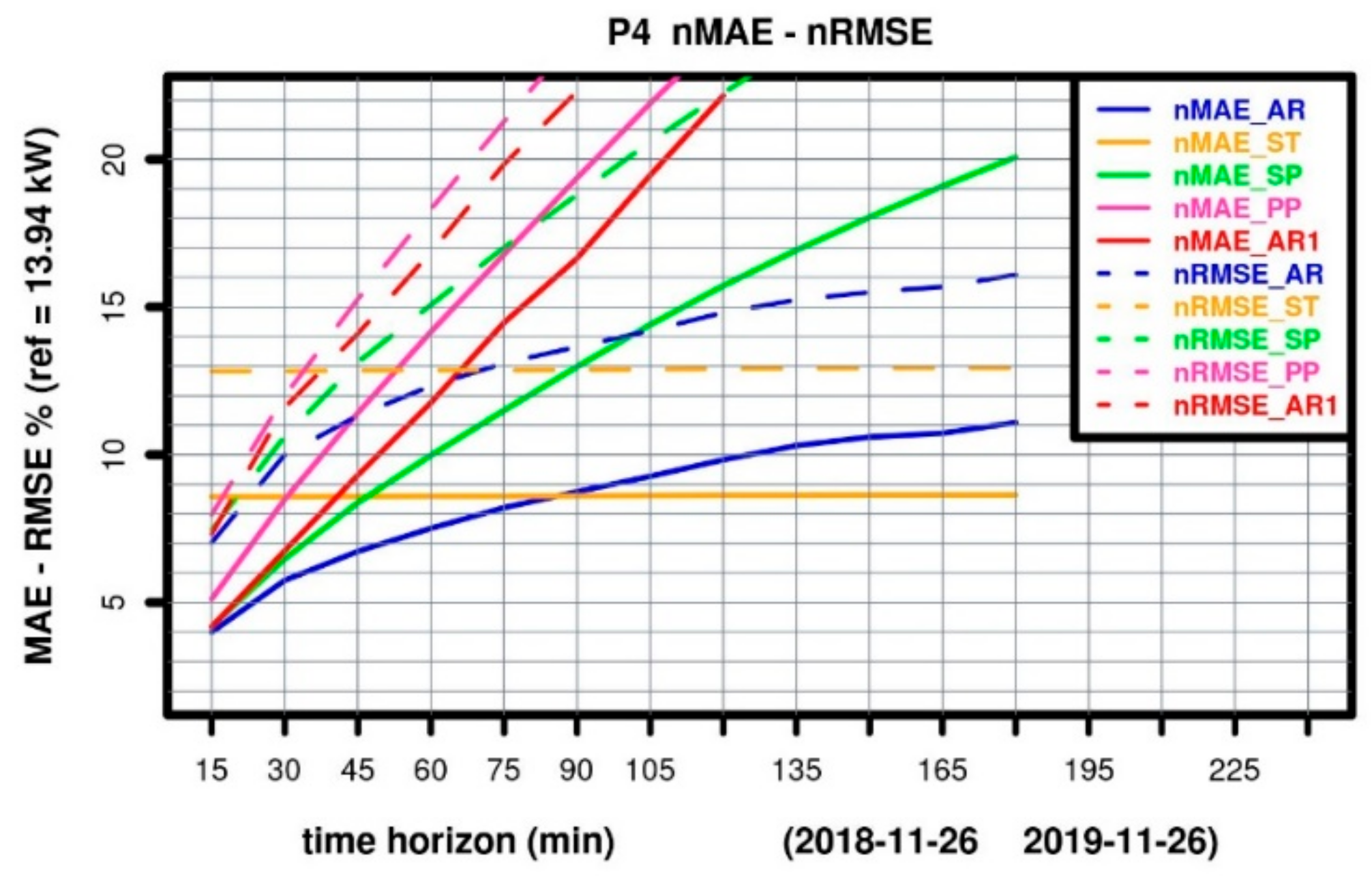
In order to give evidence of the usefulness of introducing the ST as input of the VST the authors have implemented an ARIMAX without using the ST prediction as explanatory variable. This new ARIMAX is called AR1 on the follow.

In general, the performances of AR1 are substantially lower than AR at each time horizon and it also gains worse results than SP after few lead times, as can be seen analyzing the progress of nMAE and nRMSE in Figure 9, related to plant P4. In the figure, the errors related to AR1 are shown with red lines.

In addition to consider the performance of ARIMAX without the use of ST output as exogenous variable, a comparison on the absolute MAE of ST and AR has been considered, in order to analyze the influence of the errors of the ST on the final VST. For this comparison it is meant that the VST is the one obtained from AR.

In the upper part of Figure 10, the total absolute errors $Q^{ST}\left({\epsilon }_{ST}\right)$, $Q^{VST}\left({\epsilon }_{ST}\right)$ introduced in Section 2.4 are shown, while the cumulative ones $C^{ST}\left({\epsilon }_{ST}\right)$, $C^{VST}\left({\epsilon }_{ST}\right)$ are reported in the lower part of the same figure, as a function of the ST error ${\epsilon }_r^{ST}$. The graphs on the left of Figure 10a refer to plant P1 and a forecast horizon of $K=60$ min, while those on the right of Figure 10b refer to plant P4 and a forecast horizon of $K=90$ min. The red lines refer to VST, the black ones to ST forecasts.

It can be noted that when the ST forecast is accurate, the VST fails to improve the forecast, but the associated amount of error, which is roughly twice that of the ST, is small. It should be noted that low errors can result from accurate forecasts, most often during sunny days, but also when the energy involved is small, more likely for very low sun elevation angles.

When the ST errors increase, the VST errors are definitively smaller than those of the ST, and the cumulative trends show an improvement of about 30% for the 60-min forecast horizons and around 20% for the 90-min horizons. The ability of VST to reduce ST errors is evident for any amount of ST error.

4. Discussion and Conclusions

In this work both a new short-term and a new very-short-term PV power forecasting systems have been implemented and their performances analyzed by means of the application to four small scale grid-connected plants in Italy in the period November 2018–November 2019. The ST model is mainly characterized by a multimodel approach, obtained through the exploitation of the weather forecast derived from different NWP models and an optimal combination of single forecasting systems based on the AnEn statistical technique.

The new VST system, operated by means of the ARIMAX method, stands out, in particular, for the use of the ST prediction, SP and GHI-Sat as exogenous input.

In the same study a simple, powerful prediction method has been also introduced, that is an “astronomical” correction of the pure persistence, obtained through a normalization of the solar zenith angle along the time.

Both the optimized multimodel ST and the VST have gained promising results, outperforming the respective references at each time horizon of the forecast. In particular, in terms of nMAE, the ST has obtained an improvement at least greater than 30% with respect to the smart persistence, used as baseline and of around 40% in terms of nRMSE, for each of the three day-ahead forecasting horizon.

As regard the VST the improvement with respect to the baseline is always relevant, for each horizon and rapidly increases with the time-frame. This successful result derives from the exploitation of the output of the ST as exogenous input of ARIMAX, as shown by means of a comparison with another version of ARIMAX, without the use of the ST as explanatory variable.

Through the use in combination of the ST and VST forecasts, a multi-time frames forecasting tool has been realized, covering the horizon from fifteen minutes up to three days ahead with a time resolution of fifteen minutes. Both the ST and VST are well suited for operational use for their reduced request of computing power. The VST is able to start at any time of the day and because of its speed of execution it can supply continuously updated and more accurate forecasts. Both the methods do not require historical and current weather measurements in situ, resulting easy to apply when this information is not available.

The multi-time frame tool has obtained good performances for all the plants, different from each other for size, orientation and climatic conditions of the places where they are installed, proving that they can be generalized and adopted on various plants, with no requirement of specific information on the installation. It is also important to take in account that the methods have been applied to small-scale plants, highly sensitive to changes in cloudiness conditions, therefore further improvements in the performances are expected when applied to larger plants. It is in fact well known the effect of smoothing error due to an increase in spatial scale studied by Pierro et al. [41].

The influence of the weather variability on the performances has been investigated by means of a specific analysis of the cloudiness variation in correspondence of each site. The analysis has confirmed that it is not proper to expect that a PV power forecasting method could obtain the same performances regardless of the meteorology of the place where it is applied. Therefore, it can be useful, in general, to complement the error analysis with a study of the weather conditions of each site.

With regard to the ST, other optimization systems are under study, that could lead to further improvements, while for the VST other information on the cloudiness, derived from meteorological satellites, not only in correspondence of the site but also in the surroundings, could help to capture irradiance variations in advance.