Article

A Low-Voltage DC Backbone with Aggregated RES and BESS: Benefits Compared to a Traditional Low-Voltage AC System

1
EELab/Lemcko, Department of Electromechanical, Systems and Metal Engineering, Ghent University, 8500 Kortrijk, Belgium
2
EELab, Department of Electromechanical, Systems and Metal Engineering, Ghent University, 9052 Ghent, Belgium
3
FlandersMake@UGent—Corelab EEDT-DC, Flanders Make, 9052 Ghent, Belgium
*
Author to whom correspondence should be addressed.
Submission received: 25 January 2021 / Revised: 19 February 2021 / Accepted: 23 February 2021 / Published: 4 March 2021
(This article belongs to the Special Issue Load Modelling of Power Systems)

Abstract

:
The increasing penetration of PV into the distribution grid leads to congestion, causing detrimental power quality issues. Moreover, the multiple small photovoltaic (PV) systems and battery energy storage systems (BESSs) result in increasing conversion losses. A low-voltage DC (LVDC) backbone to interconnect these assets would decrease the conversion losses and is a promising solution for a more optimal integration of PV systems. The multiple small PV systems can be replaced by shared assets with large common PV installations and a large BESS. Sharing renewable energy and aggregation are activities that are stimulated by the European Commission and lead to a substantial benefit in terms of self-consumption index (SCI) and self-sufficiency index (SSI). In this study, the benefit of an LVDC backbone is investigated compared to using a low-voltage AC (LVAC) system. It is found that the cable losses increase by 0.9 percent points and the conversion losses decrease by 12 percent points compared to the traditional low-voltage AC (LVAC) system. The SCI increases by 2 percent points and the SSI increases by 6 percent points compared to using an LVAC system with shared meter. It is shown that an LVDC backbone is only beneficial with a PV penetration level of 65% and that the BESS can be reduced by 22% for the same SSI.

1. Introduction

The increasing concern about climate change has incited the European Commission to set up a European Green Deal. The Green Deal provides an action plan to make the economy more sustainable—e.g., by the efficient usage of resources and moving to a clean and circular economy. The key target for 2030 is to achieve a share of renewable energy sources (RES) of at least 32% and an improvement in the energy efficiency by at least 32.5% [1]. It is obvious that this will lead to an energy landscape which will be highly dominated by wind and photovoltaic (PV) energy. Today, many residential and industrial distribution grid users have already installed PV on their roof. However, at the moment more than 90% of usable rooftops all over Europe are still unused [2].
The increasing penetration of PV into the distribution grid can lead to increasing congestion. This congestion could be translated towards higher energy losses and impact on power quality aspects, such as voltage rise and voltage unbalances, which constrain the PV hosting capacity. The many single-phase connected PV systems are causing unbalanced voltage variations at each phase, resulting in power quality issues in the connected appliances [3]. Concrete cases are already established in certain regions in Germany, where, due to the increase in RES, voltage and capacity issues are occurring [4]. Those problems can be avoided by implementing flexible solutions, such as demand response, battery storage, or a combination of them. A more radical solution is to reinforce the grid. It is the task of the Distribution Network Operator (DNO) to face this challenge and weigh up the cost for flexibility and grid reinforcement [5]. The study [6] investigated the impact of renewable energy sources in the European distribution grid by 2050. It was found that in general, for distribution grids with a share of RES higher than 60%, grid reinforcement is more cost-effective. Additionally, the expected massive shift from internal combustion engine-based vehicles to electrical vehicles (EV) exposes the distribution grid as well to many power quality-related issues. Similar to the issues related to the increasing PV penetration, this causes the necessity to primarily fully exploit the flexibility potential and, if absolutely necessary, reinforce the grid [7].
Low-voltage DC (LVDC) distribution systems are gaining more and more attention due to their many benefits. In [8], the power transfer capability was analysed and it was found that, with the same cable, a 1.28 times greater power could be transported by DC compared to the same system using AC. It is important to mention that for AC a traditional three-phase 400 V AC system was considered, while for DC a unipolar 800 V DC or a bipolar ±400 V DC system was used. Given that, for AC, a four-wire cable was considered, the power transfer capability could even be 2.56 when using two wires in DC in parallel for the positive and zero pole. A higher DC voltage would further increase this benefit. Consequently, for a unipolar DC system with two wires the maximal power can be transferred over a cable length that is 1.80 times longer without violating the maximal voltage drop.
As many household appliances such as EV chargers as well as distributed energy resources (DER) operate on DC, the converter stage could be eliminated. Converters contain semiconductors and capacitors, which are prone to failure. Consequently, the reliability and lifetime of these systems will increase. Secondly, due to the elimination of the conversion stage the system will be more efficient [9]. In [10], a loss analysis was conducted on a case with 20 residential houses with a community PV system and a gas engine co-generation unit. The comparison of the losses was carried out with these assets connected to a distribution system operating on 200 V AC and a system operating on ±200 V DC. The whole losses of the DC system are around 15% lower than those of the LVAC system. The same analysis [11] was conducted but only with a community PV system and an apartment with 20 residential units, operating on the same AC and DC voltage. The most interesting result of this analysis is the fact that an improvement in the efficiency is only achievable for PV installations larger than 11 kW, which produce around 12% of the consumption on a yearly basis.
Notwithstanding all these advantages, LVDC systems still have to face many challenges. Firstly, there is a lack of commercially available products such as converters and protection devices. Protection devices designed for AC rely on the natural zero-crossing of the AC current. For LVDC systems, effective protection could be achieved by using electronic-based protection devices, which are more expensive [12].
Today, almost no DC-compatible household appliances exist. It is obvious that a complete shift to LVDC will need investments and will take considerable time. Secondly, for a smoother development of those products, standardisation is needed on, for instance, the voltage level. The maximum voltage applicable for LVDC systems is 1500 V, as specified in the IEC 60038 [13]. It should be mentioned that there is no single voltage that might fit all devices, as it often depends on the application. The optimal voltage level could be optimised by a trade-off of the following system parameters: efficiency, cost, and safety [14]. In [15], a voltage of ±350 V is proposed for high loads, such as electric vehicles or PV installations. At the same time, this voltage could be used to connect household appliances, as the conversion losses will be lower due to the low voltage difference compared to the AC amplitude voltage of 325 V.
As has already been mentioned, a radical shift to LVDC in the distribution system and the residential load will take much time and investment. A hybrid structure is today more feasible and could pave the way for a gradual transition [
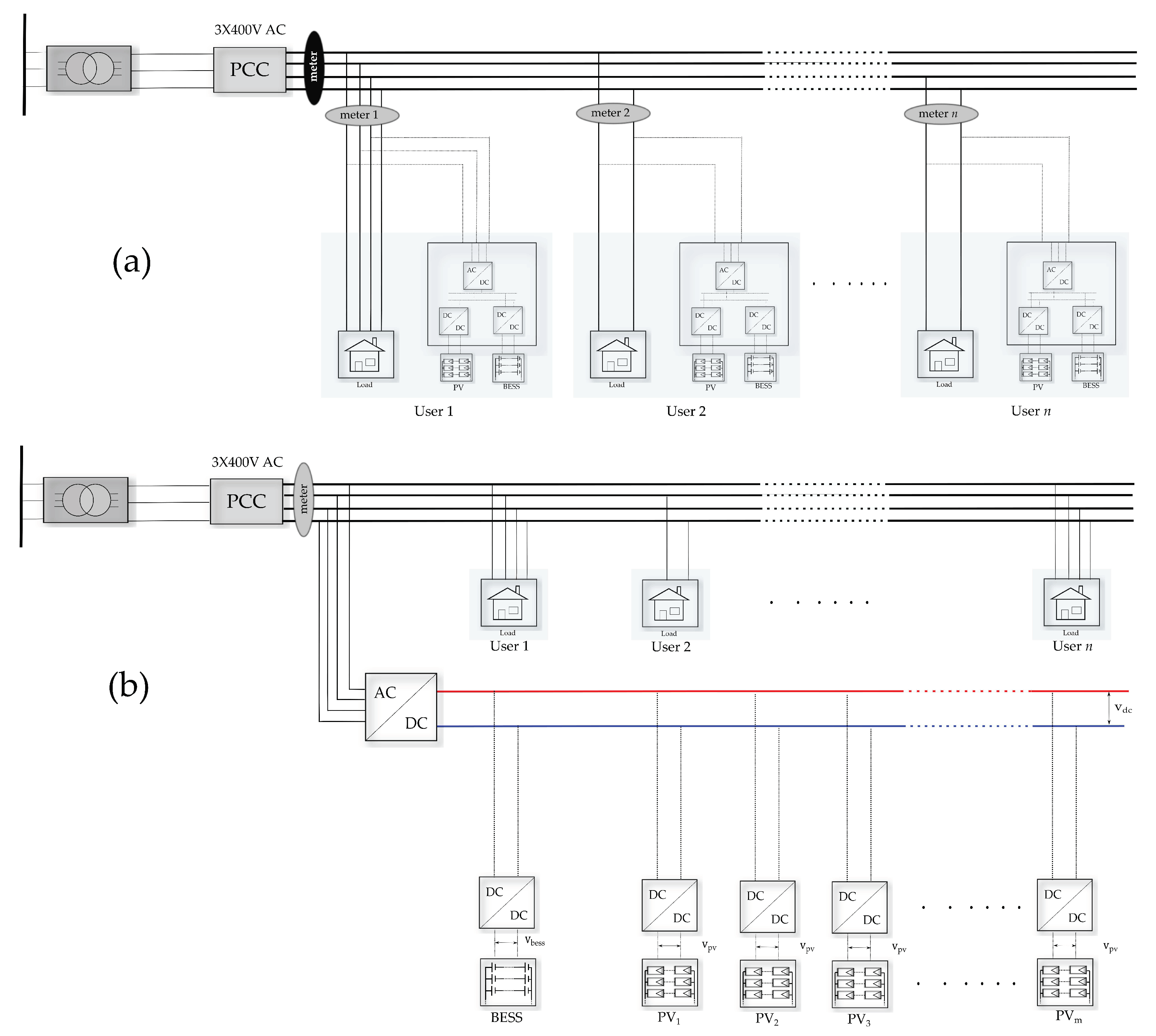
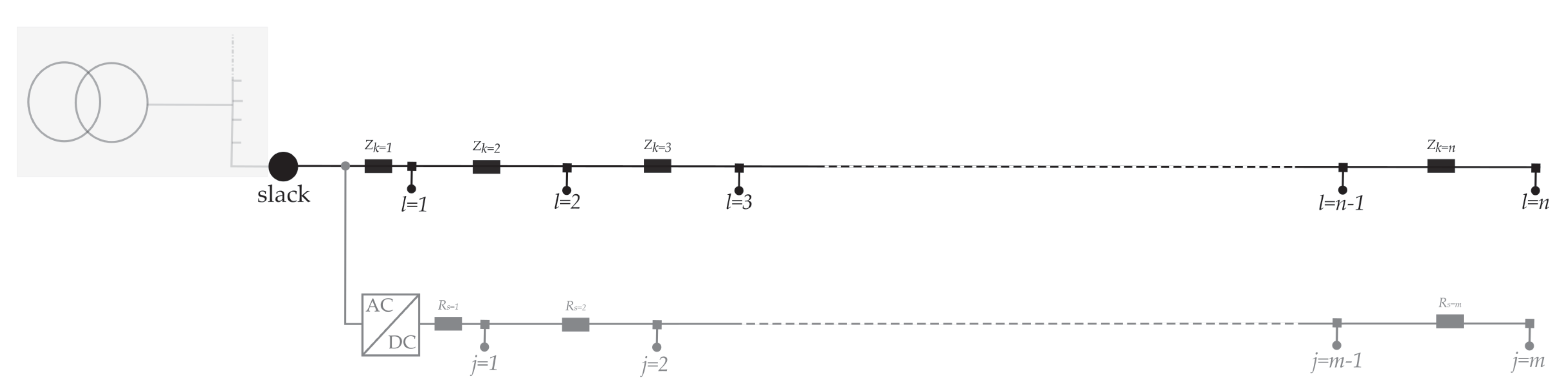
16]. In this article, a grid architecture is presented where the load is connected on a traditional low-voltage AC (LVAC) system while the PV installations and battery energy storage system (BESS) are connected to an LVDC backbone. This architecture is especially applicable in urban areas with clusters of town houses or apartments. Instead of having a PV installation for every individual grid user with a DC/AC inverter each, one larger PV installation is applied on the roofs for every building cluster and connected on the LVDC backbone. The same applies for the BESS, as a larger BESS is connected to the LVDC backbone instead of multiple small BESSs. The LVDC backbone is connected to the point of common coupling (PCC) of the LVAC system via one large DC/AC inverter. Hence, the PV and BESS connected to the LVDC backbone could be considered as a shared asset to provide the aggregated load demand on the AC side.
By aggregating residential loads, a larger share of the total load could be covered by the produced PV energy—i.e., the self-sufficiency index (SSI) increases. At the same time, this leads to a minimal storage need for the same SSI [17]. In [18] the benefit of shared PV and BESS compared to individual PV and BESS is evaluated based on the historical load data of 21 houses. This was achieved by analysing the share of the produced energy that is directly consumed by the individual or aggregated load—i.e., the self-consumption index (SCI). The SCI increases by 15 percent points when the PV energy is shared compared to in individual PV installations. When BESS and PV are shared, the SCI increases by 11 percent points compared to individual BESS and PV. The study [19] demonstrated by a very in-depth analysis, based on a set of distribution networks containing different realistic communities, the benefit of community BESS. It was found that a community BESS could be sized 35% smaller than an individual BESS for the same SSI. A shared PV installation can be very interesting for apartment residents. The large roof areas can offer economies of scale and the aggregation of the different residential loads leads to an increase in the SCI. An Australian study [20] showed that the SCI could increase by up to 30% when aggregating 25 apartment residents. The higher the aggregation level, the higher the increase in SCI compared to the SCI for an individual grid user. However, the study also also showed that, from a certain aggregation level onwards, the SCI starts to saturate, which means that the benefit of aggregation decreases.
A higher aggregation level leads to a higher load factor, which could be explained by the fact that the baseload increases proportionally but the peak demand increases non-proportionally due to the non-synchronity of the peaks. Moreover, the six parameters describing the load duration curve of an aggregated load demand show a denser distribution as the aggregation level increases. This would make the demand more predictable and so improve the flexibility potential of the community [21,22,23]. The aggregation of demand and sharing of generation and storage are activities that are stimulated by the European Union (EU), aiming at incentivising citizens in order to get them involved in the energy market. The EU presented in 2019 in their Clean Energy Package two new actors: Renewable Energy Communities (RECs) and Citizen Energy Communities (CECs) [24]. It is not within the scope of this article to discuss the legal aspects of these new actors more in detail. However, it is important to notice the evolution to a more collective approach in the energy system, both in the legal framework and in the rising number of pilot projects in that context [25]. The aim of this study is to investigate the benefits of an LVDC backbone in a community compared to a traditional AC grid. The possible benefits could be divided into the following aspects:
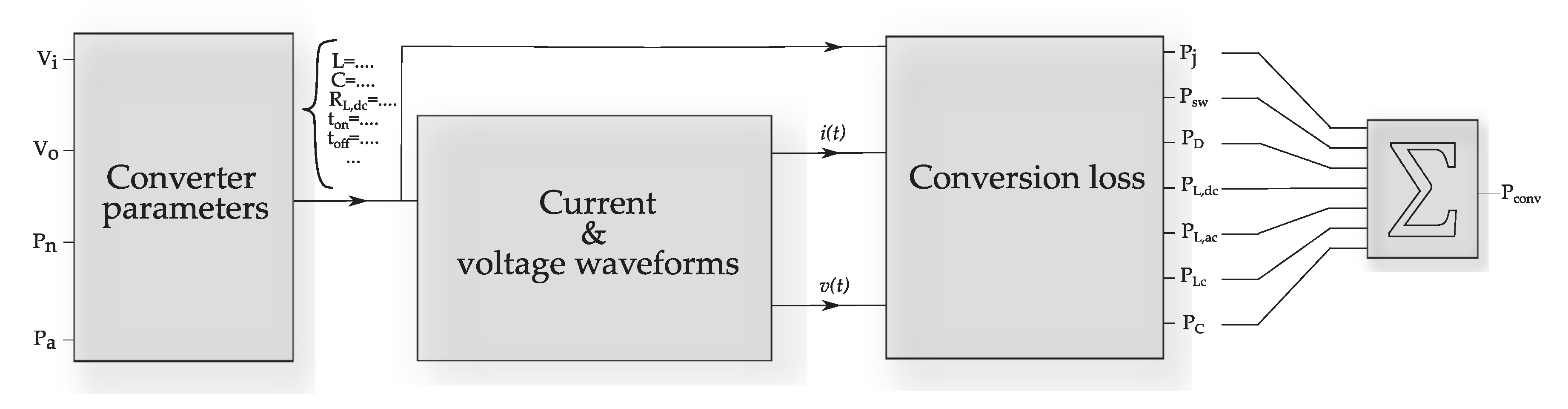
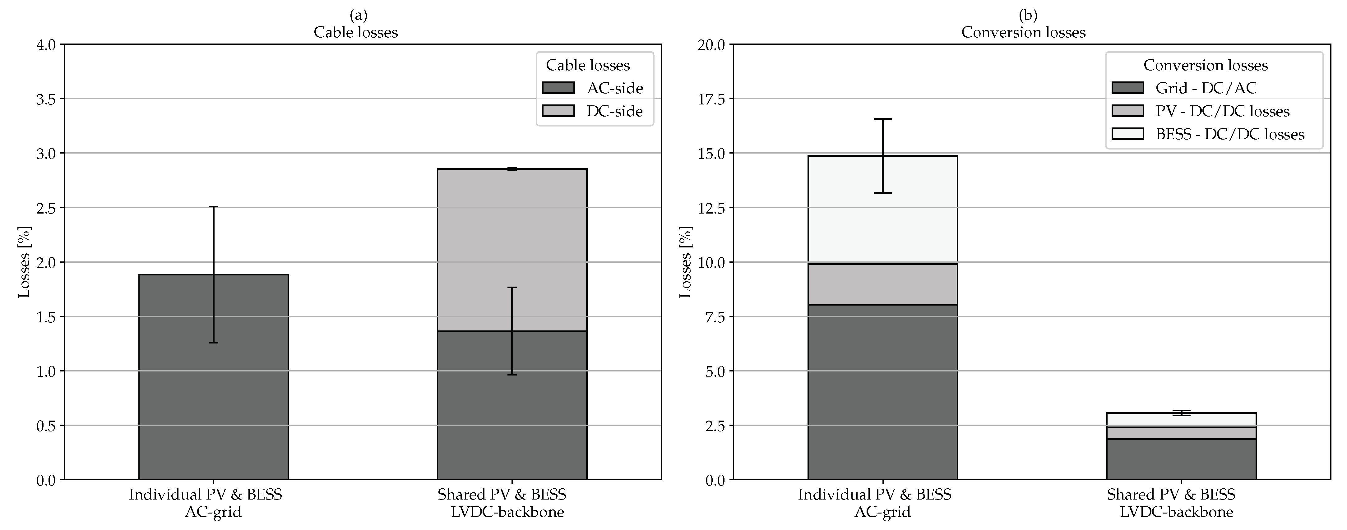
  • Conversion and cable losses: As has already been discussed, in an LVDC backbone grid architecture the number of converters is highly reduced. However, the number of conversion stages is the same compared to a traditional AC grid. The multiple small DC/AC inverters are replaced by one common inverter. The comparison of both will be performed based on converter loss models. Secondly, the cable losses will be analysed for both architectures. In a traditional AC grid, the produced and stored energy can be directly consumed by the grid user, while for an architecture with an LVDC backbone additional cable losses occur on the DC side. Nevertheless, the losses can be reduced due to the higher operating DC voltage and the reduced unbalance.
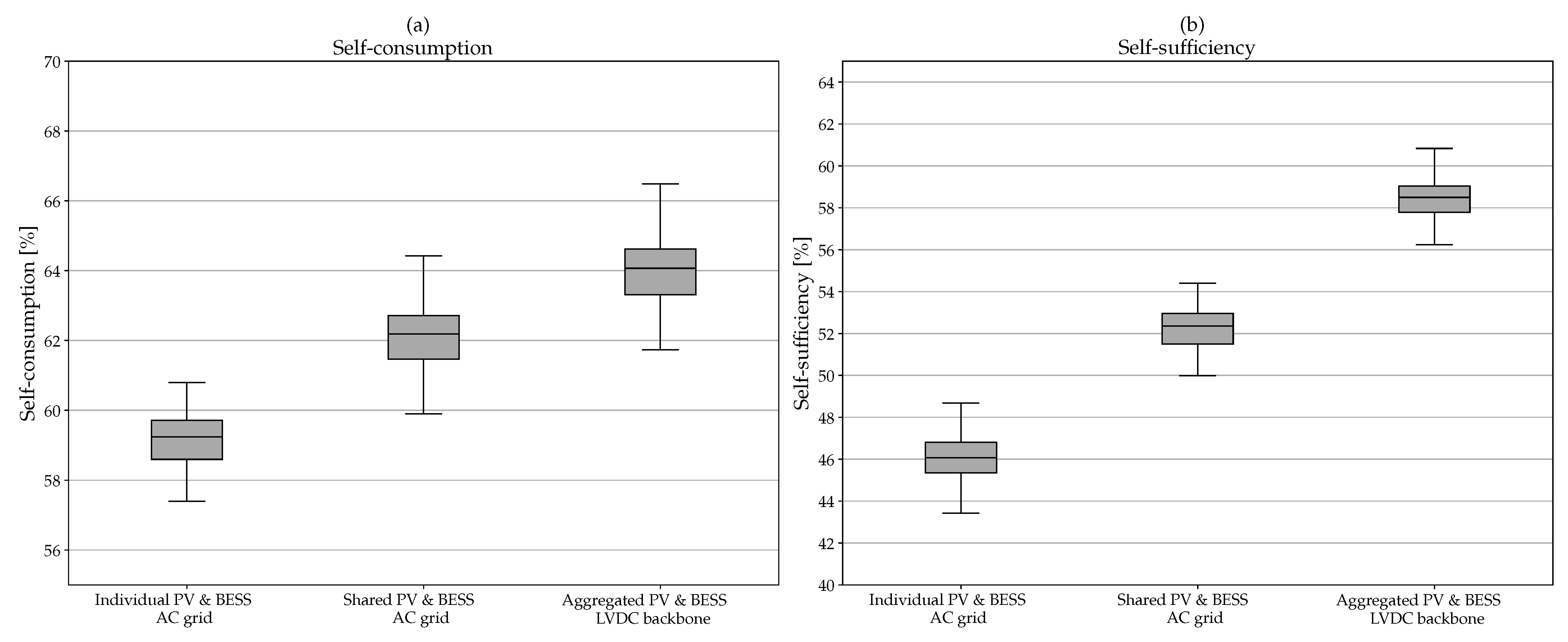
  • SCI and SSI: It has been shown in various other works that the aggregation of demand and sharing of PV and BESS increases the SCI and SSI. In this work, this will be analysed taking into account the cable and converter losses that occur. This will be carried out for three situations: a traditional AC architecture with individual PV and BESS (i) without energy sharing and (ii) with energy sharing, as well as (iii) an LVDC backbone architecture with energy sharing.
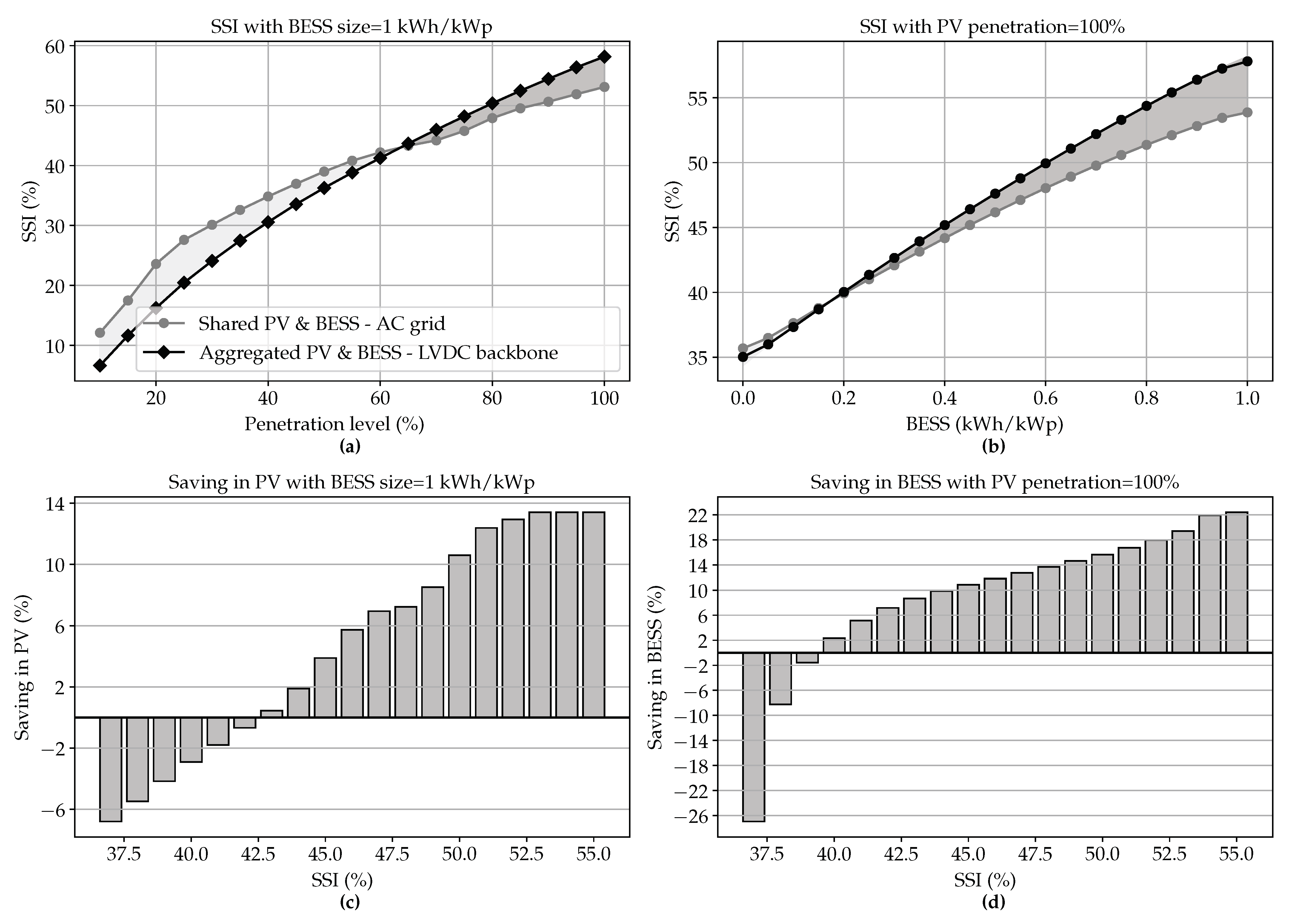
  • Savings in assets: The savings in PV and BESS are here analysed for an LVDC backbone compared to a traditional AC grid with individual PV and BESS and the possibility to share energy. The savings will be calculated assuming, as a starting point, that the same benefits in terms of SSI should be achieved as with a traditional AC architecture with energy sharing. The savings in assets could be translated into a saving of materials and therefore an environmental benefit.
In Section 2, the analysed grid architectures as well as the case study are presented. The consumption data and the solar irradiance data used in the study and the applied methodology for calculating the power losses and the SCI and SSI are discussed in Section 3. The LVDC backbone voltage applied in the study is determined based on an efficiency optimisation in Section 4. In Section 5, the final results are presented and discussed. Finally, further research aspects and conclusions are formulated in Section 6 and Section 7.

2. Studied Systems

2.1. Grid Architectures

The architectures that will be studied in this article are shown in Figure 1.
Individual PV and BESS on AC grid without the possibility to share energy (Figure 1a): Every household has its own energy meter so that the energy provider can invoice the household pro rata their electric consumption. The produced PV energy of each household that has not been directly consumed or stored is injected into the grid. As the feed-in tariff is declining every year or even phased out in some countries, it is assumed in this study that the grid user could only benefit from the self-consumed energy [26].
Shared PV and BESS on AC grid with the possibility to share energy (Figure 1a): The grid is considered as a closed distribution grid and its users forms a community. Hence, the community is considered as a single entity connected to the grid, with one single meter measuring the net consumed energy. The community will be invoiced pro rata their net consumed energy, and this cost will be divided among the participants according to their real consumption.
Shared PV and BESS on LVDC backbone (Figure 1b): The same for this architecture, however, the PV and BESS are now connected to a unipolar LVDC backbone. Instead of having small individual PV installations and BESS, a larger community PV installation as well as a community BESS is foreseen.

2.2. Case Description

For this study, a community size of 25 members is considered, as shown in Figure 2. In [27], it has been proven that, for aggregation levels higher than 20, the benefit increase for the community in terms of SSI and SCI is negligible. Moreover, based on data provided by the Flemish DNO Fluvius and originating from a suburban area, 75% of low-voltage distribution feeders have a maximum of 25 connections. Specifically for urban areas, the number of connections in feeders is typically between 15 and 25 when considering detached and semi-detached houses [28]. The community consists of 24 residential members and one small or medium-sized enterprise (SME).
The heterogeneity of members is supported by the Renewable Energy Directive (RED) and the Internal Electricity Market Directive (IEMD) in the context of providing “environmental, economic or social benefits for its shareholders or members or for the local areas where it operates, rather than financial profits” [29]. Secondly, SMEs often have a certain potential for PV due to their relatively large roof area and a load profile that is complementary to residential load profiles. The residential members consist of ten town houses and two apartment blocks with 8 and 6 apartments, which have each their own metered grid connection.
All the buildings are considered to be suitable for PV. To calculate the potential of PV, a monocrystalline PV module of Yingli (YL230 P-29b) is considered with a peak power of 230 W. A tilt angle of 35 ° and an azimuth angle of 180 ° are selected as the most appropriate configuration for the building roofs. The potential for PV is presented in Table 1.
The total cable length is identical for both grid architectures. The cable length between the different AC-connections of the houses is considered 10 m. For the LVDC backbone architecture, the cable lengths are shown in Table 1. It should be noted that when an AC grid architecture is considered, every grid user has its own PV installation as well as an individual BESS. The PV capacity on the roof is subsequently divided between the users proportional to their annual energy consumption (see Section 3.5).

3. Materials and Methods

3.1. Flowchart

Before the methodology is explained more in detail, a flowchart of the process is presented in Figure 3. When considering a traditional AC grid architecture, the process is started by populating the AC grid by randomly selected residential consumption profiles and one single SME consumption profile (Figure 3a). Thereafter, the appropriate individual PV and BESS systems are sized. Then, how the considered grid user is connected to the grid—i.e., the type of connection and, if single-phase, the connected phase—is assessed. Based on this information, a parameter table is drawn up with parameters as the in- and output voltage of the converter or information regarding the grid connection. If this information is known, the conversion losses and cable losses can be calculated and the SCI and SSI of each individual grid user can be assessed for one complete year. This process is repeated for every node, and once this is done for the 25 nodes the results are stored in a table and a new iteration is started.
For an LVDC backbone architecture (Figure 3b), the PV and BESS system is sized according to the aggregated consumption. After determining the conversion losses from the DC/DC converters, a DC power flow analysis is performed in order to compute the cable losses on the DC side. Afterwards, the losses due to the DC/AC-inverter are calculated. Before computing the cable losses on the AC side, the type of connection as well as the connected phases of the grid users on the AC side are defined. Finally, the SCI and SSI are calculated and stored and a new iteration is started. Similarly, the losses, the SCI, and SSI are computed for a complete year. This process is repeated for 100 iterations. The number of iterations is chosen as a compromise between the computation time and representativeness of the analysis. Both analyses are performed with a time horizon of one year. The calculation is run on a computer with Intel(R) Core(TM) i7-8850H CPU with a speed of 2.6 GHz and an installed RAM of 16 GB. The total computation time amounts to 41,760 s (11.6 h) for computing the AC grid architecture and 1100 s (0.31 h) for computing the LVDC backbone architecture.

3.2. Conversion Loss Model

Several approaches exist for modelling converters. However, it should be mentioned that an extensive converter model requires a large computation effort without assuring an adequate accuracy. This is due to the lack of accurate models of generally available commercial devices. Secondly, an advanced model is quite excessive for merely computing the losses. In this work, a quasi-static approach is applied which is sufficiently accurate for this purpose while requiring low computation efforts. The use of this method means that certain effects that are less significant for loss calculations are neglected in this study [30]. A few of these effects are listed below:
Effects of temperature on device phenomena. In this article, a constant temperature of 25 ° C has been assumed.
The dynamics that occur at higher frequencies due to parasitics as they have a time scale that is typically much shorter than the switching period.
Other dynamics related to the switching phenomena, such as the diode reverse recovery and the tail current of the switch.
Evaluating the power losses of converters according to the quasi-static approach entails a model that carries out the calculation of the several losses dependent on the input voltage V i , the output voltage V o , the nominal power P n , and the actual power P a (Figure 4). Based on the first three input parameters, the converter can be accordingly sized following the parameters and formulas provided in Appendix A. The current and voltage waveforms, i ( t ) and v ( t ) , are reconstructed using the principles described in [31,32] and coded in Python with the aid of the library UliEngineering. By using the quasi-static approach, the losses are computed over a single switching cycle of the concerning converter and then accumulated over a time equal to the time period of the AC grid sinewave. Once the instantaneous power loss over a time period is obtained, these losses are averaged.
Figure 5 displays the different considered converters in this work. The DC/DC buck converter steps down the input voltage while the bidirectional converter steps up the input voltage for a positive current (as shown) and steps it down for a negative current. The topology of the DC/DC bidirectional converter is based on a converter implemented in a real test setup with a BESS connected on a common DC-bus with variable voltage (see Appendix A.5). The DC/AC inverter converts a DC voltage to an AC voltage. All these conversions are accompanied by certain losses.
The mathematical formulations of these losses are given below for every component. A description of the used symbols of the converter parameters can be found in Appendix A. The auxiliary self-consumption of the converter as well as the standby losses have been neglected in this study.
Switching losses P s w : These losses occur during the transition phase of the switching state and depend on the voltage V S across the switch and the current I S flowing through the switch. The faster the switching element switches on or off, the lower the switching losses. The higher the switching frequency or parasitic capacitance, the higher these losses [33].
P s w = 1 2 I S V S ( t o n + t o f f ) f s + 1 2 C O S S V s 2 f s
Conduction losses P j in the switching elements: In the model, MOSFETs are considered as switching elements. These elements have a certain on-state resistance which causes conduction losses when the switch current with waveform i S ( t ) is flowing. The time period of the switching cycle is represented by T s .
P j = R D S , o n 1 T s 0 T s i S ( t ) 2 d t
Conduction losses P D in the diodes: The same applies for the diodes. However, the losses occuring in the diodes are often smaller than those occuring in the switching elements [34].
P D = 1 T s 0 T s i S ( t ) V F + i S ( t ) 2 r T d t
Core losses P L c in the inductor: As no materials exhibit a perfect magnetic response, losses occur in the core when the magnetic flux B changes. Thus, there is no direct proportionality with the magnitude of the current. The calculation of these losses is based on the approach of the generalised Steinmetz equation and is calculated per volume unit [35]. The improved Steinmetz parameter is obtained by Equation (5), with ω t representing the angular frequency.
P L c , V = 1 T s 0 T s k i d B d t α Δ B β α d t
k i = k ( 2 π ) α 1 0 2 π cos ω t α 2 β α d ω t
DC conduction losses P L , d c in the inductor: Due to the DC resistance of the windings, conduction losses occur. I L is the current flowing through the inductor.
P L , d c = R L , d c I L 2
AC conduction losses P L , a c in the inductor: Skin effects occur due to the high switching frequency, causing the resistance R L , d c to increase. It should be noted that here only the AC component of the current I L , a c is taken into account. Secondly, a constant current density is assumed in the current flowing part of the conductor.
P L , a c = R L , a c I L , a c 2
R L , a c = ρ l c π r c 2 π ( r c 1 π σ μ 0 f s ) 2
Conduction losses P C in the capacitor: Capacitors have a certain equivalent seriea resistance which represents conduction losses. The current flowing through the capacitor is represented by i c . The capacitor design parameters can be found in Table A5.
P C = R C 1 T s 0 T s i C ( t ) 2 d t .

3.3. Consumption Profiles

This study will be performed on the basis of a dataset of almost 1700 load profiles obtained by the Flemish DNO Fluvius. These load profiles originate from a suburban area and are logged through an automatic measurement reading during one year with a resolution of 15 min. For representing the residential consumers, the load profiles that comply with the Eurostat classification are used—i.e., profiles with a year consumption between 1000 kWh and 15,000 kWh [36]. Furthermore, the load profiles of SMEs are extracted from the dataset. Finally, the residential and SME load profiles are collected in a pool and during every iteration 25 profiles (24 residential and 1 SME) are selected to be analysed. In order to obtain an analysis that is representative of a large number of types of consumers, this process is repeated for 100 iterations and then represented as a distribution. In Figure 6, the distributions of the annual consumption for the individual residential consumers, the SMEs, and the aggregated consumption are displayed.
The distribution for individual residential consumers is clearly a left-skewed relatively dense distribution with a median of 3750 kWh (Figure 6a). The boxplot showa the interquartile range (q25–q75) and the outliers, and is overlayed by a scatter. As the SME load profiles are less represented, and as they inherently exhibit a high variance due to their different activities, a large spread is observed with a median of about 7830 kWh (Figure 6b). The distribution of the aggregated consumption has multiple skews and a quite large spread with a median of 107.9 MWh (Figure 6c).

3.4. PV-BESS System

The in-plane irradiance is calculated using the Hay & Davies transposition model [37]. As input data, the global horizontal irradiance, diffuse irradiance, and direct normal irradiance are needed. These data are provided by the Belgian Royal Meteorological Institute (RMI) together with the wind speed at a 10 m height and the ambient temperature. The time resolution of the dataset is 10 min, but it is resampled to 15 min in order to match the load data. PVLib, an open source Python library, is used to calculate the DC power output [38]. As mentioned previously, the PV installations will be oriented to the south with a tilt angle of 35 ° , which delivers the maximal yield for Belgium [39]. It is assumed that the PV installations are not exposed to shading due to obstacles. Local variations in the irradiance caused by moving clouds are assumed to be equal for the whole site.
Regarding the BESS, a battery with a C-rate of 1 has been considered in the simulation. Furthermore, as there is a certain dependency between the voltage and the state of charge (SoC) for Li-ion batteries, this has been taken into account in the proposed model in [40]. The relation between these parameters is shown in the curve below (Figure 7) and is implemented in the simulation model.
The PV and BESS system size depends on the individual consumption for a traditional AC grid architecture and on the aggregated consumption for an architecture with an LVDC backbone. For the latter, the sized PV system is spread over the j buildings in proportion to their roof surface and only one large BESS is foreseen. Furthermore, in order to investigate later on the sensitivity of the PV and BESS size, a sizing factor ζ is used. This is shown in Table 2.

3.5. System Voltage

The nominal output voltages of the battery and the PV systems as well as the DC voltage are important parameters for the design of converters, their conversion efficiency, and the cable losses. The selected voltages are shown in Table 3 and discussed below:
Battery voltage:
Single- and three-phase system: When looking at the market nowadays, two general centres of gravity are observed: low-voltage systems of 48 V and high-voltage systems in the range of 400 V. While 48 V batteries are widely available and accepted as standard for the telecommunication market, high-voltage systems can have different voltages. This makes 48 V more adequate, as it can be parallelised with existing systems, combined with other battery technologies, or easily be replaced [41,42,43]. Moreover, this voltage is within the range of the extra-low-voltage class defined by the IEC 60038. Consequently, those systems have a lower risk of electric shock than high-voltage systems. It should be noted that this voltage is the nominal voltage.
LVDC backbone: For larger systems, 48 V cells are stacked in a string configuration in order to obtain the desired voltage. Examples of such battery stacks and how they are configured can be found in [44,45].
PV voltage:
Single- and three-phase system: The Flemish regulation, the Synergrid C10/11 states that for peak powers of DER larger than or equal to 5 kVA a three phase connection is committed [46]. Small systems (<5 kVA) are here configured with five panels per string while larger systems (≥5 kVA) have ten panels per string. Knowing that the voltage for maximal power of the considered module type is 29.5 V, this leads to the voltages shown in Table 3.
LVDC backbone: For larger PV systems, the number of panels in series is further increased to 24 to obtain higher voltages in order to limit the cable losses.
DC voltage:
Single- and three-phase system: A unity amplitude modulation index ( m a = 1 ) is considered in this work to calculate the DC-bus voltage of the inverter. This is based on research [31] done in that field, were it has been found that overmodulation ( m a > 1 ) leads to a considerable increase in third harmonics in the current, which increases the current in the neutral conductor as well as the harmonic distortion of the voltage at grid side. At the other hand m a < 1 leads to a higher current and voltage harmonic distortion [47,48].
LVDC backbone: As already discussed before, the operation voltage level of LVDC systems is today a matter of debate. A trade off has to be made between reliability, safety, cost, and efficiency. For the presented LVDC architecture, the efficiency aspect is related to the cable losses but also to the conversion losses. The latter is very dependent on the nominal voltage the battery and the PV system is operating on. The optimal voltage level for maximal efficiency will be determined and used in the further analysis.

3.6. Power Flow Analysis

The aim of the power flow analysis is to compute the occurring cable losses. Therefore, a feeder model has been developed and populated with customers, represented by their power consumption. The consumption profiles obtained from the DNO, and collected iteratively in a pool, has been used for this purpose. No information about the type of connection, single-phase or three-phase, as well as the phase connection of the single-phase customer, has been delivered. For that reason, the type of connection has been exposed to a certain degree of randomness. However, as already discussed, for PV inverters of 5 kVA a three phase connection is committed. It is thus assumed that customers with an inverter power ≥5 kVA have their loads connected to the three phases in order to comply with the requirement of not having an unbalance between the phases larger than 5 kVA [46]. For systems smaller than 5 kVA, or when no PV is considered at all on AC-side, the type of connection is determined randomly based on a numerical distribution. This distribution is based on a dataset delivered by Fluvius containing the maximum power drawn from the grid as well as the type of connection for almost 34,000 customers without PV. As can be seen in Table 4, as the peak power increases the probability of having a single-phase connected customer decreases. For three-phase connected customers, the household load is considered to be symmetrical distributed over the three phases.
Single-phase loads and especially single-phase PV systems cause distribution systems to be unbalanced. Voltage unbalance has many detrimental impacts, such as an increase in losses in the transformer and in the cables [49]. It is thus necessary to perform a three phase power flow analysis to be able to accurately estimate these losses. A straightforward single-phase representation of the system to compute the power flow is exempted. For this work the system is decomposed into symmetrical components and then solved by the forward-backward sweep (FBS) power flow method for the power flow calculation at the AC-side [50]. The feeder is modelled by a primitive impedance matrix containing the self-impedances as well as the mutual impedances. For the DC-side, the power flow is also computed by the FBS method considering the resistance of the line. For both cases the slack bus is defined as the beginning of the feeder as shown in Figure 8 [51].
The output result of the power flow analysis is represented by the following collection sets:
i x , y ( t ) = { i 1 , y ( t ) , i 2 , y ( t ) , , i p , y ( t ) }
u x , y ( t ) = { u 1 , y ( t ) , u 2 , y ( t ) , , u p , y ( t ) }
Z = { Z 1 , Z 2 , , Z n }
R = { R 1 , R 2 , , R m }
y [ 1 , 2 , , 100 ] ; t [ 0 , 1 , , 35,040 ] ;
x [ 0 , 1 , 2 , 3 ] ; for ac grid
x = 0 ;   for LVDC backbone
Equations (10) and (11) represent the currents and voltages over the network, for every line x and for every iteration y. These are calculated with the assumption that the power factor is 0.95. The p currents and voltages are computed for every timestep t, with p = n for the AC grid and p = m for the LVDC backbone. For the LVDC backbone a unipolar network topology is considered. Additionally, also the impedances and resistances in Equations (12) and (13) are considered as outputs for the calculation of the losses. In Equation (14), the range of the parameters x, y and, t are shown. The power flow is analysed on a 15 min resolution, thus an array with size 35,040 x p will be obtained as result for the currents and voltages for every conductor for a complete common year. The parameters of the network used for the simulation of the power flow and the calculation of the losses are indicated in Table 5. It should be mentioned that the appropriate cable size is selected from the table in Appendix A.4 according to the largest current flowing in the network [52]. The authors do not rely on the typical feeder cable sections used in Flanders’ low voltage grid, in order to obtain an adequate comparison between the architectures with respect to the current density. The current ratings and resistances are based on buried cables with soil temperature of 20 °C with laying depth of 0.7 m conform the Belgian standard NBN HD603. The cable temperature is assumed to be constant.

3.7. Loss Calculation

The conversion losses are calculated for every converter separately considering variables such as the voltages or the produced power.
P D C D C , B E S S ( t ) = P c o n v ( v i , b e s s ( t ) , v o , d c , P m , P a ( t ) )
P D C D C , P V ( t ) = P c o n v ( v i , p v ( t ) , v o , d c , P m , P a ( t ) )
P D C A C , g r i d ( t ) = P c o n v ( v i , d c , v o , a c , P m , P a ( t ) )
The nominal power P n depends on the sizes of the systems, which are determined in Table 2. The losses occurring in the bidirectional DC/DC converter of the BESS P D C D C , B E S S ( t ) , the DC/DC converter of the PV system P D C D C , P V ( t ) , and the DC/AC inverter P D C A C , g r i d ( t ) are summed to obtain the total energy conversion losses.
E c o n v = t = 1 35 , 040 ( P D C D C , B E S S ( t ) + P D C D C , P V ( t ) + P D C A C , g r i d ( t ) ) · 0.25
This process is repeated during every iteration y for every selected load profile P c o n s , l ( t ) , and the result is stored in a 100 × 1 array. The same approach is applied for the cable losses. These are computed for every line and summed in order to obtain the total cable losses. Note that this is an element-wise (⊙) operation. For an architecture with individual assets, this is calculated as follow during every iteration:
E c a b l e , t o t , a c = t = 1 35,040 x = 0 3 i x , y ( t ) 2 R · 0.25
For an architecture with shared assets on an LVDC backbone, the cable losses are calculated for the AC-part and for the DC-part (second part of Equation (22)) separately with for the DC-part x = 0 .
E c a b l e , t o t , b b = t = 1 35,040 x = 0 3 i x , y ( t ) 2 R · 0.25 + t = 1 35,040 i x , y ( t ) 2 2 · R · 0.25

3.8. SCI and SSI

The SCI represents the share of the produced PV energy that is instantly consumed or stored in the BESS. This is expressed by the ratio of instantly consumed or stored PV energy, excluding the occurring conversion losses P c o n v , l ( t ) , to the total produced energy. The SSI represents the share of the energy consumption that is instantly supplied by the PV installations or the BESS, excluding the occurring conversion losses. For an architecture with individual assets without energy sharing these indexes are expressed as shown below:
S C I l = t = 1 35,040 m i n ( P p v , l ( t ) , P c o n s , l ( t ) + P B E S S , c h , l ( t ) ) P c o n v , l ( t ) P p v , l ( t )
S S I l = t = 1 35,040 m i n ( P p v , l ( t ) , P c o n s , l ( t ) + P B E S S , d i s c h , l ( t ) ) P c o n v , l ( t ) l = 1 n P c o n s , l ( t )
For an architecture with individual assets but with the possibility to share energy, the l individual consumption profiles, PV profiles and BESS charge profiles are aggregated and the SCI and SSI is calculated in the same manner but including the AC cable losses P c a b l e , t o t , a c ( t ) .
S C I = t = 1 35,040 m i n ( l = 1 n P p v , l ( t ) , l = 1 n ( P c o n s , l ( t ) ) + P B E S S , c h , l ( t ) ) P c o n v ( t ) P c a b l e , t o t , a c ( t ) l = 1 n P p v , l ( t )
S S I = t = 1 35,040 m i n ( l = 1 n P p v , l ( t ) , l = 1 n ( P c o n s , l ( t ) ) + P B E S S , d i s c h , l ( t ) ) P c o n v ( t ) P c a b l e , t o t , a c ( t ) l = 1 n P c o n s , l ( t )
When the PV systems and BESSs are aggregated on an LVDC backbone, the SCI and SSI are calculated as follow:
S C I = t = 1 35 , 040 m i n ( j = 1 m P p v , j ( t ) , l = 1 n ( P c o n s , l ( t ) ) + P B E S S , c h ( t ) ) P c o n v ( t ) P c a b l e , t o t , b b ( t ) j = 1 m P p v , j ( t )
S S I = t = 1 35,040 m i n ( j = 1 m P p v , j ( t ) , l = 1 n ( P c o n s , l ( t ) ) + P B E S S , d i s c h ( t ) ) P c o n v ( t ) P c a b l e , t o t , b b ( t ) l = 1 n P c o n s , l ( t )

4. Optimal Voltage Level

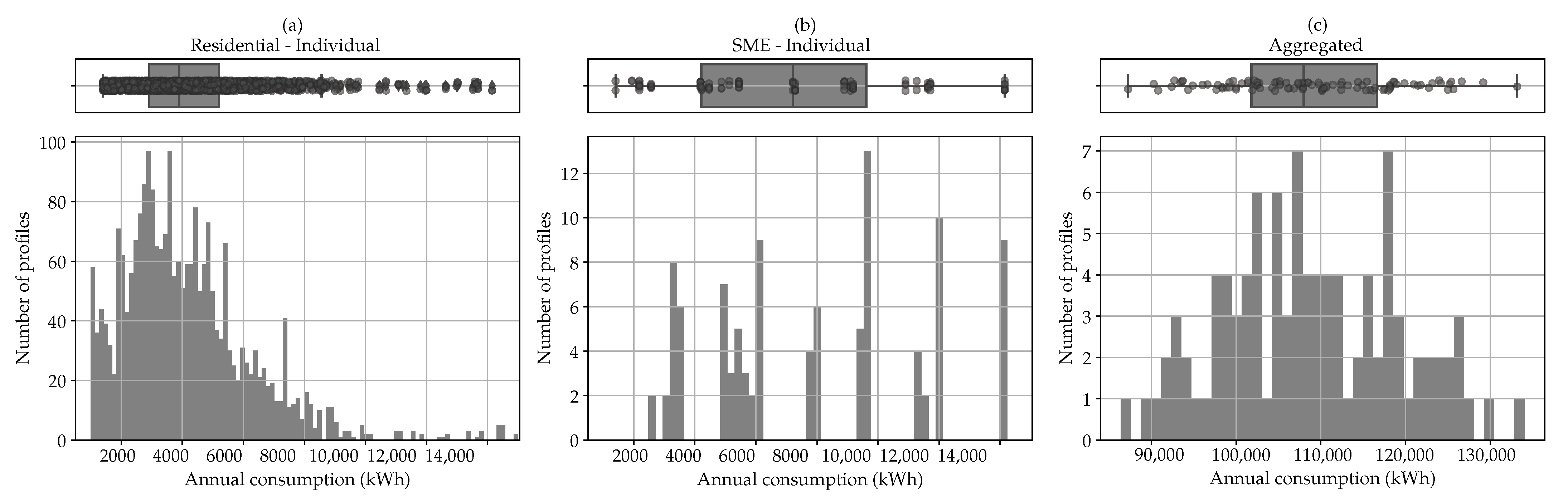
For this study, the determination of the optimal voltage level is confined to the efficiency aspect. A holistic approach taking into account, e.g., the safety aspect or the economic aspect, for the determination of the optimal voltage is certainly a requirement in the light of the development of such grid architectures in the near future as well as the establishment of the according standards. Moreover, as already discussed, the efficiency optimal backbone voltage depends strongly on the system voltages. This implicates that a case-by-case approach is required therefore, or at least a classification in function of the system scale. However, the system voltages selected in this study are surely representative for grid systems of this order of magnitude. For the median aggregated load of 107.9 MWh and ζ = 1 the installed PV power amounts 107.9 kWp and the BESS capacity amounts 107.9 kWh.
The voltage is directly related to the power transfer capability; the higher the voltage, the more power can be transferred with the same cable. Inversely, when the power is considered constant, a higher voltage leads to a lower current and a smaller required cable section. The cable section is sized according to the maximum cable ampacity delivered by the manufacturer and shown in Appendix A.4 with the additional condition that the voltage in the network does not exceed the imposed voltage limit. Due to lack of international or national standards, this voltage limit is based on the Finish SFS-6000 standard which limits the DC voltage to the range –25% to +10% [53]. Secondly, this voltage limit is assumed as a compromise to minimise the conversion losses whilst installing an affordable and, from practical point of view, a manageable cable.
In 
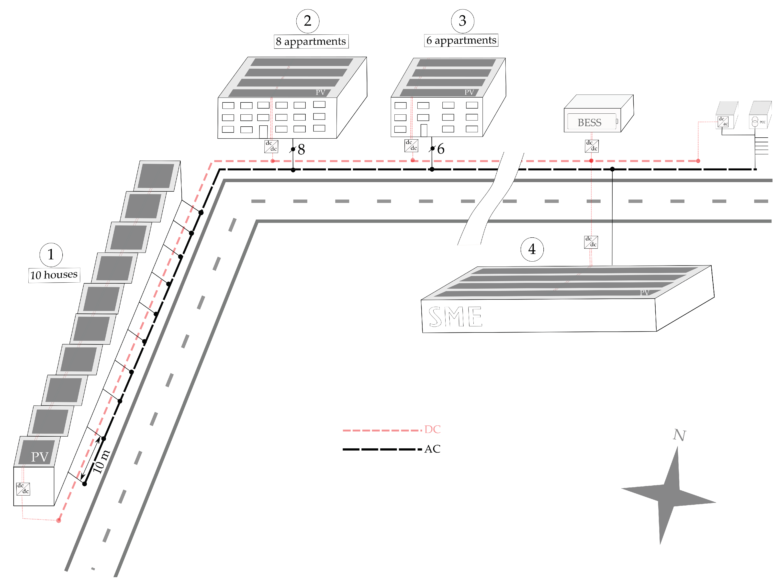
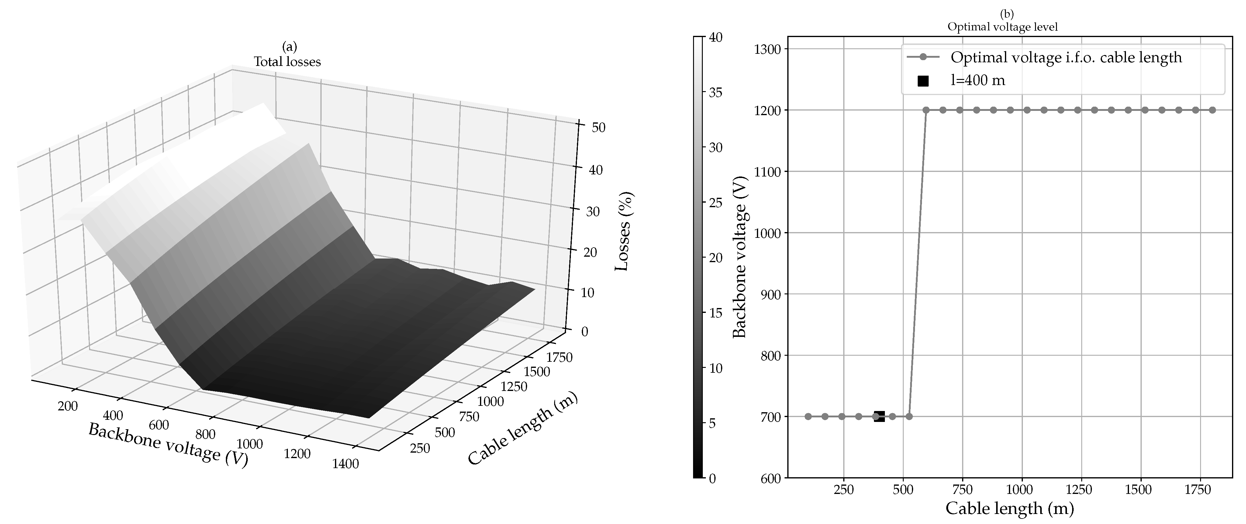
Figure 9a, the median of the losses at DC-side is plotted in function of the backbone voltage and the total cable length for the presented case. The length of the cable between the different connections is in proportion with the cable lengths given in Table 1. The analysis is limited to voltages within the upper limit level of 1500 V imposed by the IEC 60038 standard for LVDC [54]. A margin of 100 V has been applied for eventual voltage rise. It is obvious that a low voltage leads to considerable higher conduction losses. As the voltage increases the conversion losses are manifesting to a higher extent, which can be explained by the increasing voltage ratio. Although, for longer cables the cable losses are manifesting on a higher degree. This is clearly perceptible in Figure 9b, while the optimal voltage amounts 700V for cable lengths up to 525 m, for longer cable lengths the optimal voltage amounts 1200 V. For a cable length of 400 m, the optimal voltage is 700 V and the losses are almost 4.5% of the total produced or discharged energy.

5. Results and Discussion

5.1. Conversion and Cable Losses

In this paragraphm the occurring losses are analysed from the slack bus on to the end of the AC feeder and the LVDC backbone with sizing factor ζ = 1 . As the analysis is performed 100 times on a dataset selection of 25 consumption profiles, the results are shown as a distribution. When comparing the cable losses in Figure 10a, it is noticed that on AC-side the losses decrease with at least 0.5 percent points for an LVDC backbone architecture. This is due to the absence of PV injection and the many single-phase PV installations on AC-side causing voltage unbalances and thus, an increasing homopolar current which causes increasing cable losses in the neutral conductor. The losses at DC-side are very significant and leads to an unfavourable energy balance regarding the cable losses, compared to the traditional AC grid. There is no self-consumption at DC-side, except the BESS on the second last node. As a consequence the peak power transported by the LVDC backbone is high, resulting in high currents and, given the quadratic relation, much higher losses. Secondly, for the traditional AC grid the losses gradually rise for every node starting from the end of the feeder, while on the LVDC backbone the current of the aggregated PV system flows in a larger part of the cable. Overall, the losses for an LVDC backbone architecture are 0.9 percent points lower.
Regarding the conversion losses shown in Figure 10b, the energy savings are very substantial. A reduction of at least 12 percent points is observed. First, the favourable system voltages play an important role to this. Due to the low voltage ratio, the several conduction losses as well as the switching and core losses are minimal. Furthermore, the larger scale of the system ensures a better efficiency. This can be explained by the fact that the switching and core losses are not proportional to the scale of the system. The on-state resistance R D S , O N of the MOSFET declines at a faster rate than the increase rate of the continuous drain current I c . The opposite applies for the switching times t o n and t o f f , it increases at a slower rate than the continuous drain current. This can be seen in the table added in Appendix A.2. The core losses of the inductor are basically independent on the magnitude of the current but on the derivative of the magnetic flux density. Larger systems within e.g., the range of 100 kW have relatively less switching and core losses than smaller systems of e.g., 3.8 kW. Analysis of the share of the conversion losses of every converter reveals that the DC/AC-inverter losses reduce from 8% to 1.8% and the BESS DC/DC converter losses reduce from 4.9% to 0.6%. The energy savings for these converters is relatively higher than for the PV DC/DC-converter for which the losses reduce from 1.8% to 0.5%. The higher loss reduction for the DC/AC-inverter and the BESS DC/DC-converter is the result of the larger scale and the lower voltage ratio.
The error bars in the plot represent the 25th (q25) and 75th (q75) percentile of the distribution. It should be noted that, for the conversion losses, the error bars represent the variance of the total conversion losses. For the losses on AC-side, regardless the grid architecture, the variance is quite considerable. Conversely, for the losses on DC-side the variance is very small to negligible. This can be attributed to the relatively denser distribution (of the aggregated consumption shown in Figure 6) compared to individual consumers. Moreover, the sizing of the converters differs less for an LVDC backbone architecture than for a traditional AC grid. In Appendix B the power flows as well as the loss profiles for a cloudy winter day and a sunny summer day are shown for both architectures considering arbitrarily selected load profiles.

5.2. SCI and SSI

As already discussed, aggregating load consumption and allowing energy sharing within a community creates benefits in terms of SCI and SSI. When a traditional AC grid is considered with individual meters the median of the SCI is, as shown in Figure 11a, 59%. If the produced energy as well as the BESSs is shared—i.e., a community is created with shared meter—the SCI increases by 3 percent points to 62%. Aggregation of PV and BESS on an LVDC backbone leads to a further increase in the SCI to 64%, caused by the significant increase in the conversion efficiency. When considering only the interquartile range (q25–q75), the spread is quite similar for the three situations and there is no overlap, which means that an increase in SCI is very probable. Although, the minimum and maximum in the three situations overlaps. For an LVDC backbone architecture the maximum decrease is about 2.5 percent points while the maximum increase is 6.6 percent points compared to an AC grid with shared meter.
The SSI, which is in fact a measure of the purchased energy from the grid, increases substantially (Figure 11b). For a traditional AC grid with individual meters, the median of the SSI amount 46%. An increase in more than 6 percent points is achieved for an AC grid with shared assets and 12.5 percent points for an LVDC backbone architecture. As there is no overlap between the distributions (q0.35–q99.65), it could be stated with high certainty that an LVDC backbone has a benefit compared to a traditional AC grid. These significant benefits are the consequences of aggregating the consumption and the decreased conversion losses. When aggregating different consumption profiles the load factor increases compared to an individual consumption profile. This is mainly due to the general non-synchronity of the daily peak demand between individual users [21]. As the size of the PV system for an AC grid with shared assets and for an LVDC backbone is proportional to the aggregation level, the increase in the SCI is not as high as the increase in the SSI.

5.3. Saving in BESS and PV

Until now, the analysis has only been based on a 100% PV penetration level and a BESS capacity of 1 kWh per kWp PV. In order to investigate for which PV or BESS sizes an LVDC backbone is beneficial, a sensitivity analysis is performed. The analysis consists of a calculation of the SSI for the traditional AC grid architecture with shared PV and BESS and an LVDC backbone with aggregated PV and BESS. The PV penetration level defines the percentage of grid users having a PV installation, or when an LVDC backbone architecture is considered, the ratio of the PV produced energy to the aggregated consumption. Figure 12a shows that for systems with PV penetration level lower than 64% an LVDC backbone architecture is not beneficial. The additional cable losses on the DC-side are then more significant as well as the increasing conversion losses due to the smaller converters. The increase rate of the SSI declines for both architectures with increasing PV penetration level since more PV surpluses cannot be consumed directly.
The relationship of the BESS size, expressed in kWh/kWp, and the SSI is shown in Figure 12b. A slight declining increase rate of the SSI is observed with increasing BESS. This is mainly due to the seasonal character of the solar irradiance. However, the rate is declining much faster for the AC grid architecture than for the LVDC backbone architecture. This can be attributed to the fact that for larger BESS sizes the conversion efficiency increases due to the scale effect. For BESS smaller than 0.18 kWh/kWp, a LVDC backbone is not beneficial, the conversion efficiency is lower and the cable losses at DC-side are having the upper hand.
It has already been proven in this study that an LVDC backbone architecture leads to an increase in the SSI for PV and BESS sizes that are large enough. Inversely, it can be stated that these assets could be sized smaller while resulting in the same SSI as the AC grid architecture, which means that on annual basis the same amount of energy has to be purchased from the grid. The SSI has been considered in this analysis as it is easily translatable to an economic value. When considering a BESS size of 1 kWh/kWp (Figure 12c) a saving in PV is achievable when the minimal desired SSI is 43%. As the desired SSI increases, the saving in PV increases too until it reaches a maximum realisable saving of 13.5% for a SSI of 53%. As the BESS size is proportional to the installed PV capacity it is obvious that the same saving can be achieved for the BESS capacity. In Figure 12d the saving in BESS is represented for a grid with a PV penetration level of 100%. A saving in BESS can be achieved when the minimal desired SSI is 40%. As the desired SSI increases, the potential saving in BESS increases gradually. Important to notice is that an LVDC backbone is not beneficial when no BESS is foreseen. This can be translated to the fact that the saving in conversion losses of the BESS has a significant contribution to the total saving. The maximum saving is achieved when a SSI is desired of 55%, the saving is than 22% compared to the needed BESS in a traditional AC grid with shared meter for the same desired SSI. These results exhibit the possible benefit of an LVDC backbone in urban areas with high PV penetration level.

6. Further Investigation

It has been proven that the LVDC backbone architecture has many benefits, especially in terms of SSI and conversion efficiency. This grid architecture has the potential to be implemented in existing grids where the distribution cable is highly congested and a reinforcement is needed. A second possible application are new districts where the penetration of PV is expected to be high. Furthermore, the LVDC backbone could also be a way to optimise the electrical vehicle (EV) infrastructure integration in the low voltage distribution grid. Advantages of EV integration on DC are inter alia simplified control and better efficiency [55,56]. These advantages could be quantified during later investigations.
An important parameter related to the efficiency is the voltage level. This has been considered as a constant 700 V in order to obtain maximal efficiency. However, a dynamic voltage level could possibly be more efficient given the inherent voltage variations of the PV installations and BESSs. In a future work a voltage optimisation control will be set up and the dynamic voltage solutions will be studied. More generally, the optimal voltage level should also be assessed to following aspects: safety, reliability and cost. After all, the usefulness of a bipolar LVDC backbone will be investigated which could be interesting when having multiple PV installations of different scale.
One of the main differences between the AC grid architecture and the LVDC backbone architecture is the number of converters. For an LVDC backbone the number of converters can be drastically reduced. Moreover, it is found that the nominal power of the converters is not proportional to its weight, which means that a larger system will have a lower specific weight than a small system (Figure 13a). As a consequence, this grid architecture contributes to the reduction in the material footprint which is promoted by the European Commission, notwithstanding the need of an additional cable [57]. The latter has to be compared with the material footprint for a reinforced AC grid with the same capabilities in order to obtain a fair comparison. Furthermore, the cable will be exposed to its maximal ampacity only during a limited number of hours a year, i.e., when the PV production is maximal in the summer. This means that the cable could eventually be sized smaller provided that the emergency ampacity would not be exceeded. Additionally, the material needed for grid connection of PV and BESS as well as the protection devices for both architectures should be compared. Based on these aspects a complete analysis could be made assessing the potential material reduction [58].
Additionally, the orientation and tilt angle of the PV installation is in this study considered the same for the whole installation. The study [59] showed that for individual consumers a benefit in terms of SSI is possible as well as lower cable losses due to lower peak power. However, it should be investigated whether a multi-oriented aggregated PV installations in a community could lead to a further increase in the SSI and a decrease in the losses in the LVDC backbone.
Finally, an economic analysis will provide insight into the feasibility of such a grid architecture, which is important for, e.g., investors, grid operators, and energy cooperatives. Only when it is proven that the investment in the infrastructure is beneficial and reduces the cost for society compared to the traditional architecture could this system be realised. This means that a total cost of ownership analysis should be performed as well as a payback analysis. These analyses should include the cost for grid connection, the system balance cost (e.g., PV modules, converters, mounting frames, and cables) as well as the labour cost. Figure 13b illustrates that the specific cost per power unit for inverters decreases as the nominal power increases, which means that a larger system is considerably cheaper than multiple small converters [43]. The cable investment cost constitutes mainly the cost for earthworks, such as the trenching or digging work, and the purchase cost of the cable. Based on data published by the Flemish DNO [60], the cost for the placement of a cable is only about 10% of the total investment cost. As a consequence, the placement of an additional cablewill not constitute a substantial share of the total cost.

7. Conclusions

In this article, the benefit of a hybrid AC/DC grid architecture with an LVDC backbone for the connection of PV and BESS has been analysed. Firstly, the optimal voltage level of the LVDC backbone was investigated. It was found that for cable lengths less than 500 m, the conversion losses take the upper hand. As a consequence, the optimal voltage is equal to the nominal voltage of the PV installation and BESS. For longer cable lengths, the optimal voltage increases in order to reduce the cable losses. Due to the optimal voltage selection, the conversion losses are drastically reduced compared to a traditional AC grid. The reduction amounts to 12 percent points. Regarding the cable losses, they increased by 0.9 percent points due to the additional cable and due to the high PV power injected into the LVDC backbone. The reduction in voltage unbalances as well as the absence of PV injection in the AC grid causes the cable losses on the AC side to reduce by 0.4 percentage points.
The SCI is found to increase by 5 percent points compared to an AC grid with individual assets and 2 percent points compared to an AC grid with shared assets. The SSI increases by 12.5 percent points compared to an AC grid with individual assets and 6 percent points compared to an AC grid with shared assets. In both the SCI and SSI, the saving in losses of the LVDC backbone have an impact. These benefits can be translated to a reduced amount of energy injected to the grid and a more significant reduction in energy purchased from the grid. The increase in SSI is only achievable for grids where the PV penetration level is higher than 64%. As the penetration level increases, the benefit of an LVDC backbone increases compared to an AC grid with shared assets. Furthermore, it has been found that for an LVDC backbone without BESS, the SSI is less favourable. Only when the BESS size is larger than 0.18 kWh per kWp installed PV, does the SSI become higher.
When a constant BESS size of 1 kWh/kWp is considered, a saving of 13.5 percent of PV capacity is realisable by aggregating PV and BESS in an LVDC backbone instead of having an AC grid with shared assets. This means that the BESS size can also be reduced to the same extent. When the PV penetration level is 100%, a saving of BESS capacity of 22% is achieved. In addition to this, the number of converters is highly reduced and only one large DC/AC inverter is needed. Based on manufacturer data, it has been found that the specific weight decreases with the increasing nominal power of the inverter. These material savings as well as the economic viability of the LVDC backbone could be further investigated in future work. However, the economies of scale of energy communities coupled with the reduction in PV and BESS size for an LVDC backbone will likely lead to a shorter payback time. This, in turn, leads to a better return on investment, and the possibly of a lower energy invoice for the members of the community.
The benefit of a dynamic voltage in terms of efficiency will similarly be investigated and a dynamic voltage optimisation control will be developed. Regarding the power quality issues in the low-voltage distribution grid caused by the high PV penetration level, this is highly reduced due to (i) the segregation of load and generation storage and (ii) the aggregation of PV and BESS on DC. After all, this study showed that the LVDC backbone architecture has various benefits and can be a solution for an optimal integration of PV and BESS, aiming at an increased SSI ofor energy communities.

Author Contributions

Conceptualisation, H.A. and J.D.; methodology, H.A. and J.D.; software, H.A.; validation, H.A.; formal analysis, H.A.; investigation, H.A. and J.D.; resources, J.D.; data curation, J.D.; writing—original draft preparation, H.A.; writing—review and editing, H.A., J.D., L.V., J.K. and R.C.; visualisation, H.A.; supervision, J.D. and L.V.; project administration, J.D., L.V. and J.K.; funding acquisition, J.D. and L.V. All authors have read and agreed to the published version of the manuscript.

Funding

This publication frames within the EMPOWER2.0 project, which receives financial support from the European Fund for Regional Development via the Interreg North Sea Region Programme. The sole responsibility for the content of this publication lies with the authors. It does not necessarily reflect the opinion of the European Union. Neither the Interreg North Sea Region Programme nor the European Commission are responsible for any use that may be made of the information contained therein. More information: https://northsearegion.eu/empower-20/ (accessed on 23 November 2020).

Institutional Review Board Statement

Not applicable.

Informed Consent Statement

Not applicable.

Acknowledgments

The authors would like to thank the Flemish distribution system operator Fluvius for providing the dataset of consumption profiles and the grid data. Secondly, the authors would also like to thank the RMI for providing the meteorological data that have been used as input for the calculation of the irradiance and the PV system model.

Conflicts of Interest

The authors declare no conflict of interest.

Appendix A. Parameters and Specifications

Appendix A.1. General Parameters

Table A1. General parameters.
SymbolParameterValue
V F Diode forward voltage1.45 V
r T Dynamic resistance0.5 m Ω
f s , d c d c Switching frequency DC/DC-converters50 kHz
f s , d c a c Switching frequency DC/AC-converters4 kHz
Δ u Maximal allowable voltage ripple5%
Δ i Maximal alowable current ripple5%
μ 0 Permeability of free-space 4 π 10 7 H/m
μ r Relative permeability of the core material256
ρ Specific resistance of the inductor winding1.68 × 10 8 Ω m
B m a x Saturated magnetic flux density of core material0.5 T
α Steinmetz material constant 11.43
β Steinmetz core material constant 21.585
kSteinmetz core material constant 315.144
σ Conductivity of the inductor winding5.96 × 10 7 S/m
A e , t y p e Effective area of the typical core279 mm2
l e , t y p e Effective length of the typical core144 mm
l e , t y p e Effective turn length of the typical conductor97 mm
l a i r Air gap length10 mm
JAllowed current density in the inductor winding2 × 10 6 A/m
KWindow utilization factor of the inductor0.5

Appendix A.2. Switch Parameters

Table A2. MOSFET parameters.
ID (A)Vce (V)RDS,ON ( Ω )ton (ns)toff (ns)Coss (nF)Type
5170016110.012C2M1000170D
1012000.285.210.80.023C2M0280120D
159000.1727250.04E3M0120090D
3510000.06520190.06C3M0065100K
7217000.04548650.171C2M0045170D
1189000.0240630.296NTHL020N090SC1
21912000.012351500.66APTMC60TLM14CAG
42312000.0042761682.57CAS300M12BM2
80017000.014857900.35SND 0800M170100
100017000.00842705701.2855SNG 1000X170300

Appendix A.3. Converter Design Equations

Table A3. Inductor design parameter calculation.
DC/DC BuckDC/DC BoostDC/AC Inverter
Inductance (mH) L = ( V i V o ) t o n Δ I m a x L = ( V o V i ) t o f f Δ I m a x L = V d c Δ I m a x m f s
Area product A p = L I m a x J K B m a x
Scale factor S f = A p A p , t y p e
Effective core length (m) l e = l e , t y p e S f
Effective core area (m3) A e = A e , t y p e S f
Total reluctance (Ampère-Turns/Wb) t = f e + a i r = l e μ 0 μ r A e + l a i r μ 0 A e
Turns N = L
Total conductor length (m) l c = l c , t y p e S f N
Winding conductor radius (m) r c = I J π
Total conductor DC resistance ( Ω ) R L , D C = ρ N L w , t y p e S f A c
Core volume (m3) V c = V c , t y p e S f 3
Table A4. Capacitor design parameter calculation.
DC/DC BuckDC/DC Boost
Capacitor (F) C = Δ I m a x 8 f s Δ V m a x
Equivalent serie resistance ( Ω ) R C = Δ V m a x Δ I m a x

Appendix A.4. Cable Parameters

Table A5. Maximal permissible current I z and cable resistance r t for EAXVB cable.
A (mm 2 ) I z (A) r t ( Ω /km)
351400.868
501650.641
702050.443
952450.32
1202800.253
1503150.206

Appendix A.5. Test Setup Bidirectional BESS DC/DC Converter

Figure A1. Specifications of the real test setup.
Energies 14 01420 g0a1

Appendix B. Power Flows and Losses Visualisation

Appendix B.1. Traditional AC Grid Architecture

Figure A2. Visualisation of the total power flows and losses for the AC grid architecture with (a) the power flows and (b) the conversion and cable losses for a cloudy day in the winter and (c) the power flows and (d) the conversion and cable losses for a sunny day in the summer.
Energies 14 01420 g0a2

Appendix B.2. LVDC Backbone Architecture

Figure A3. Visualisation of the total power flows and losses for the LVDC backbone architecture with (a) the power flows and (b) the conversion and cable losses for a cloudy day in the winter and, (c) the power flows and (d) the conversion and cable losses for a sunny day in the summer.
Energies 14 01420 g0a3

References

  1. 2030 Climate & Energy Framework. Available online: https://ec.europa.eu/clima/policies/strategies/2030_en (accessed on 1 November 2020).
  2. Hemetsberger, W.; Schmela, M.; Beauvais, A.; Breyer, C. 100% Renewable Europe: How to Make Europe’s Energy System Climate-Neutral before 2050; SolarPower Europe: Brussels, Belgium, 2020; pp. 8–14. [Google Scholar]
  3. Patil, A.; Girgaonkar, R.; Musunuri, S.K. Impacts of increasing photovoltaic penetration on distribution grid—Voltage rise case study. In Proceedings of the 2014 International Conference on Advances in Green Energy (ICAGE), Thiruvananthapuram, India, 17–18 December 2014; Volume 10, pp. 100–105. [Google Scholar]
  4. Bayer, B.; Matschoss, P.; Thomas, H.; Marian, A. The German experience with integrating photovoltaic systems into the low-voltage grids. Renew. Energy 2018, 119, 129–141. [Google Scholar] [CrossRef]
  5. Klyapovskiy, S.; You, S.; Michiorri, A.; Kariniotakis, G.; Bindner, H.W. Incorporating flexibility options into distribution grid reinforcement planning: A techno-economic framework approach. Appl. Energy 2019, 254, 113662. [Google Scholar] [CrossRef] [Green Version]
  6. Allard, S.; Debusschere, V.; Mima, S.; Tuan, T.Q.; Hadjsaid, N.; Criqui, P. Considering distribution grids and local flexibilities in the prospective development of the European power system by 2050. Appl. Energy 2020, 270, 114958. [Google Scholar] [CrossRef]
  7. Clement-Nyns, K.; Haesen, E.; Driesen, J. The Impact of Charging Plug-In Hybrid Electric Vehicles on a Residential Distribution Grid. IEEE Trans. Power Syst. 2010, 25, 371–380. [Google Scholar] [CrossRef] [Green Version]
  8. Agustoni, A.; Borioli, E.; Simioli, G.; Tironi, E.; Ubezio, G. LV DC distribution network with distributed energy resources: Analysis of possible structures. In Proceedings of the 18th International Conference and Exhibition on Electricity Distribution (CIRED 2015), Turin, Italy, 6–9 June 2005; Volume 18, pp. 6–9. [Google Scholar]
  9. Yang, S.; Bryant, A.; Mawby, P.; Xiang, D.; Ran, L.; Tavner, P. An Industry-Based Survey of Reliability in Power Electronic Converters. IEEE Trans. Ind. Appl. 2011, 18, 480–486. [Google Scholar]
  10. Kakigano, H.; Miura, Y.; Ise, T. Loss evaluation of DC distribution for residential houses compared with AC system. In Proceedings of the 2010 International Power Electronics Conference (ECCE ASIA), Sapporo, Japan, 21–24 June 2010; pp. 480–486. [Google Scholar] [CrossRef]
  11. Kakigano, H.; Miura, Y.; Ise, T.; Van Roy, J.; Driesen, J. Basic Sensitivity Analysis of Conversion Losses in a DC Microgrid. In Proceedings of the International Conference on Renewable Energy Research and Applications (ICRERA 2012), Nagasaki, Japan, 11–14 November 2005; pp. 1–6. [Google Scholar] [CrossRef]
  12. Emhemed, A.A.S.; Burt, G.M. An Advanced Protection Scheme for Enabling an LVDC Last Mile Distribution Network. IEEE Trans. Smart Grid 2014, 5, 2602–2609. [Google Scholar] [CrossRef] [Green Version]
  13. Rodriguez-Diaz, E.; Chen, F.; Vasquez, J.C.; Guerrero, J.M.; Burgos, R.; Boroyevich, D. Voltage-Level Selection of Future Two-Level LVdc Distribution Grids: A Compromise Between Grid Compatibiliy, Safety, and Efficiency. IEEE Electrif. Mag. 2016, 4, 20–28. [Google Scholar] [CrossRef] [Green Version]
  14. International Electrotechnical Commission. Technology Report LVDC: Electricity for the 21st Century; International Electrotechnical Commission: Geneva, Switzerland, 2017. [Google Scholar]
  15. Evans, M.A.V. Why Low Voltage Direct Current Grids? A Case-Study Assessment of Using Direct Current in Low Voltage Distribution; Delft University of Technology: Delft, The Netherlands, 2013. [Google Scholar]
  16. Ploumpidou, E. Supporting the Transition to DC Micro Grids in the Built Environment; Eindhoven University of Technology: Eindhoven, The Netherlands, 2017. [Google Scholar]
  17. Freitas, S.; Reinhart, C.; Brito, M.C. Minimizing storage needs for large scale photovoltaics in the urban environment. Sol. Energy 2018, 159, 375–389. [Google Scholar] [CrossRef]
  18. Luthander, R.; Widén, J.; Munkhammar, J.; Lingfors, D. Self-consumption enhancement of residential photovoltaics with battery storage and electric vehicles in communities. Energy 2016, 112, 221–231. [Google Scholar] [CrossRef]
  19. Barbour, E.; Parra, D.; Awwad, Z.; González, M.C. Community energy storage: A smart choice for the smart grid? Appl. Energy 2018, 212, 489–497. [Google Scholar] [CrossRef] [Green Version]
  20. Roberts, M.B.; Bruce, A.; MacGill, I. PV for appartment buildings: Which side of the meter? In Proceedings of the Solar Research Conference, Melbourne, Australia, 30 November–2 December 2017. [Google Scholar]
  21. Claeys, R.; Delerue, T.; Desmet, J. Assessing the influence of the aggregation level of residential consumers through load duration curves. In Proceedings of the IEEE ISGT-Europe, Bucharest, Romania, 29 September–2 October 2019; pp. 1–5. [Google Scholar]
  22. Poulin, A.; Dostie, M.; Fournier, M.; Sansregret, S. Load duration curve: A tool for technico-economic analysis of energy solutions. Energy Build. 2008, 40, 29–35. [Google Scholar] [CrossRef]
  23. Sevlian, R.A.; Rajagopal, R. A model for the effect of aggregation on short term load forecasting. In Proceedings of the 2014 IEEE PES General Meeting, Washington, DC, USA, 27–31 July 2014; pp. 1–5. [Google Scholar]
  24. Roberts, J.; Frieden, D.; d’Herbermont, S. Complie: Energy Community Definitions. 2019. Available online: https://www.compile-project.eu/wp-content/uploads/Explanatory-note-on-energy-community-definitions.pdf (accessed on 18 November 2020).
  25. Hannoset, A.; Peeters, L.; Tuerk, A. Bridge H2020: Energy Communities in the EU Task Force Energy Communities. 2019. Available online: https://www.h2020-bridge.eu/wp-content/uploads/2020/01/D3.12.d_BRIDGE_Energy-Communities-in-the-EU-2.pdf (accessed on 18 November 2020).
  26. Interreg Europe. Renewable Energy Self-Consumption: A Policy Brief from the Policy Learning Platform on Low-Carbon Economy. 2020. Available online: https://www.interregeurope.eu/fileadmin/user_upload/plp_uploads/policy_briefs/Energy_self-consumption__Policy_brief_final.pdf (accessed on 12 February 2021).
  27. Schlund, J.; Pflugradt, N.; Steber, D.; Muntwyler, U.; German, R. Benefits of Virtual Community Energy Storages compared to Individual Batteries based on Behaviour Based Synthetic Load Profiles. In Proceedings of the IEEE ISGT-Europe, Sarajevo, Bosnia and Herzegovina, 21–25 October 2018; pp. 1–6. [Google Scholar]
  28. Gonzalez, C.; Geuns, J.; Weckx, S.; Wijnhoven, T.; Vingerhoets, P.; De Rybel, T.; Driesen, J. LV Distribution Network Feeders in Belgium and Power Quality Issues due to Increasing PV Penetration Levels. In Proceedings of the IEEE ISGT-Europe, Berlin, Germany, 14–17 October 2012; pp. 1–8. [Google Scholar]
  29. Lowitzsch, J.; Hoichka, C.E.; van Tulder, F.J. Renewable energy communities under the 2019 European Clean Energy Package—Governance model for the energy clusters of the future? Renew. Sustain. Energy Rev. 2019, 122, 1–13. [Google Scholar] [CrossRef]
  30. Maksimovic, D.; Stankovic, A.M.; Thottuvelil, V.J.; Verghese, G.C. Modeling and simulation of power electronic converters. Proc. IEEE 2001, 89, 898–912. [Google Scholar] [CrossRef]
  31. Vázquz, N.; López, J.V. 11—Inverters. In Power Electronics Handbook; Rashid, M.H., Ed.; Elsevier: Tampa, FL, USA, 2018; pp. 289–339. [Google Scholar]
  32. Czarkowski, D. 10—DC-DC Converters. In Power Electronics Handbook; Rashid, M.H., Ed.; Elsevier: Tampa, FL, USA, 2018; pp. 275–289. [Google Scholar]
  33. Xiong, Y.; Sun, S.; Hongwei, J.; Shea, P.; Shen, Z.J. New Physical Insights on Power MOSFET Switching Losses. IEEE Trans. Power Electron. 2009, 24, 525–531. [Google Scholar] [CrossRef]
  34. Rafiq, M.; Hasan, M.F.U. Design and Analysis of 60 kW DC-DC Converter for Hybrid Electric Vehicle Applications. Master’s Thesis, Chalmers University of Technology, Göteborg, Sweden, 2011. [Google Scholar]
  35. Venkatachalam, K.; Sullivan, C.R.; Abdallah, T.; Tacca, H. Accurate prediction of ferrite core loss with nonsinusoidal waveforms using only Steinmetz parameters. In Proceedings of the 2002 IEEE Workshop on Computers in Power Electronics, Mayaguez, PR, USA, 3–4 June 2002; Volume 8, pp. 36–41. [Google Scholar]
  36. Eurostat. Energy Statistics—Electricity Prices for Domestic and Industrial Consumers, Price Components. Available online: https://ec.europa.eu/eurostat/cache/metadata/en/nrg_pc_204_esms.htm (accessed on 18 November 2020).
  37. Davies, J.A.; Hay, J.E. Calculation of the solar radiation incident on an inclined surface. In Proceedings of the 1st Canadian Solar Radiation Data Workshop, Toronto, ON, Canada, 17–19 April 1978; pp. 59–72. [Google Scholar]
  38. Holm, W.F.; Clifford, W.H.; Mikofski, M.A. pvlib python: A python package for modeling solar energy systems. Open Source Softw. 2018, 3, 884. [Google Scholar]
  39. Jacobson, M.Z.; Jadhav, V. World estimates of PV optimal tilt angles and ratios of sunlight incident upon tilted and tracked PV panels relative to horizontal panels. Sol. Energy 2018, 169, 55–66. [Google Scholar] [CrossRef]
  40. Erdinc, O.; Vural, B.; Uzunoglu, M. A dynamic lithium-ion battery model considering the effects of temperature and capacity fading. In Proceedings of the International Conference on Clean Electrical Power, Capri, Italy, 9–11 June 2009; pp. 383–386. [Google Scholar]
  41. PVEurope. What Goes into Designing an Effective High-Voltage Battery? Dr Vetter of the Fraunhofer ISE Explains. Available online: https://www.pveurope.eu/energy-storage/what-goes-designing-effective-high-voltage-battery-dr-vetter-fraunhofer-ise-explains (accessed on 18 November 2020).
  42. Bellini, E. Lithium Battery for Low- and Also High-Voltage Storage. Available online: https://www.pv-magazine.com/2020/06/09/lithium-battery-for-low-and-high-voltage-storage/ (accessed on 19 November 2020).
  43. Europe-Solarstore. Available online: https://www.europe-solarstore.com/batteries.html (accessed on 5 November 2020).
  44. Larson, S. Energy Storage in Utility Systems. Available online: https://na.eventscloud.com/file_uploads/05612c1b0b638b14d1ede35138c07afc_EnergyStorage_HRS_2019-02-04.pdf (accessed on 26 November 2020).
  45. Delta Electronics. Delta Lithium-ion Battery Energy Storage Container. Available online: https://filecenter.deltaww.com/Products/Download/18/1805/0803%20DM05-Container-201807.pdf (accessed on 26 November 2020).
  46. Synergrid. Specifieke Technische Voorschriften Voor Elektriciteitsproductie-Installaties die Parallel Werken met het Distributienet. Available online: http://www.synergrid.be/download.cfm?fileId=Technical_prescription_C10-11_ed2-1_20190901_tekst_NL.pdf&language_code=NED (accessed on 3 November 2020).
  47. Chicco, G.; Schlabbach, J.; Spertino, F. Characterisation and assessment of the harmonic emission of grid-connected photovoltaic systems. In Proceedings of the IEEE Russia Power Tech, St. Petersburg, Russia, 27–30 June 2005; pp. 1–7. [Google Scholar]
  48. Brenna, M.; Chiumea, R.; Gandolfi, C. Harmonic analysis: Comparison between different modulation strategies for three phase inverter connecting Distributed Generation. In Proceedings of the International Conference on Clean Electrical Power, Ischia, Italy, 14–16 June 2011; pp. 231–236. [Google Scholar]
  49. Schwanz, D.; Möller, F.; Rönnberg, S.K.; Meyer, J.; Bollen, M.H.J. Stochastic Assessment of Voltage Unbalance Due to Single-Phase-Connected Solar Power. IEEE Trans. Power Deliv. 2017, 32, 852–861. [Google Scholar] [CrossRef]
  50. Ulinuha, A.; Masoum, M.A.S.; Islam, S.M. Unbalance power flow calculation for a radial distribution system using forward-backward propagation algorithm. In Proceedings of the Australasian Universities Power Engineering Conference, Sydney, Australia, 4–7 December 2007; pp. 1–6. [Google Scholar]
  51. Kersting, W.H. Distribution System Modeling and Analysis; CRC Press LLC: Las Cruces, NM, USA, 2002. [Google Scholar]
  52. Kabelwerk EUPEN AG. Technische Gegevens Voor Energie- en Stuurstroom Laagspanningskabel 0.6/1 kV; Ed. 06/2016-08-18; EUPEN AG: Eupen, Belgium, 2016. [Google Scholar]
  53. Suomen Standardisoimisliitto. FS 6000 Sähköasennusstandardisarja; SESKO Standardization: Helsinki, Finland, 2017. [Google Scholar]
  54. International Electrotechnical Commission. IEC standard voltages. In International Standard—IEC-60038; Ed.06/2009; International Electrotechnical Commission: Geneva, Switzerland, 2009. [Google Scholar]
  55. Locment, F.; Sechilariu, M. Modeling and Simulation of DC Microgrids for Electric Vehicle Charging Stations. Energies 2015, 8, 4335–4356. [Google Scholar] [CrossRef]
  56. Aluisio, B.; Bruno, S.; De Bellies, L.; Dicorato, M.; Forte, G.; Trovato, M. DC-Microgrid Operation Planning for an Electric Vehicle Supply Infrastructure. Appl. Sci. 2019, 9, 2687. [Google Scholar] [CrossRef] [Green Version]
  57. European Commission. A New Circular Economy Action Plan for a Cleaner and More Competitive Europe. Available online: https://ec.europa.eu/commission/presscorner/detail/en/qanda_20_419 (accessed on 3 November 2020).
  58. Zhuang, X.L.; Niu, H.Q.; Zhang, Q.F.; Ye, K.F.; Sun, G.H. Experimental Study on the Emergency Ampacity of XLPE Cable and Its Application. Appl. Mech. Mater. 2014, 599, 931–934. [Google Scholar] [CrossRef]
  59. Azaioud, H.; Desmet, J.; Vandevelde, L. Benefit Evaluation of PV Orientation for Individual Residential Consumers. Energies 2020, 13, 5122. [Google Scholar] [CrossRef]
  60. Fluvius. Fluvius 2020 Elektriciteit Tariefbladen Finaal. Available online: https://www.fluvius.be/sites/fluvius/files/2019-12/fluvius-aansluittarieven-elektriciteit-2020.pdf (accessed on 3 November 2020).
Figure 1. Illustration of the considered architectures with (a) a traditional AC grid with individual BESS and PV with an individual meter or shared meter (b) and an LVDC backbone with shared PV and BESS.
Energies 14 01420 g001
Figure 2. Illustration of the studied case with an LVDC backbone.
Energies 14 01420 g002
Figure 3. Iterative process for assessment of (a) a traditional AC grid architecture and (b) an LVDC backbone architecture.
Energies 14 01420 g003
Figure 4. Conversion loss model.
Energies 14 01420 g004
Figure 5. Converter circuits: (a) is a DC/DC buck converter, (b) is a DC/DC bidirectional boost converter, and (c,d) are single- and three-phase DC/AC inverters.
Energies 14 01420 g005
Figure 6. Distribution of the annual consumption for (a) the residential individual consumption, (b) the consumption of SMEs, and (c) the aggregated consumption.
Energies 14 01420 g006
Figure 7. Battery voltage in the function of the SoC.
Energies 14 01420 g007
Figure 8. Busses and nodes in the feeder and in the LVDC backbone.
Energies 14 01420 g008
Figure 9. Optimal voltage: (a) sensitivity analysis on voltage in function of total losses and (b) optimal voltage in function of the cable length.
Energies 14 01420 g009
Figure 10. (a) Cable losses and (b) conversion losses.
Energies 14 01420 g010
Figure 11. Distribution of the (a) self-consumption and (b) self-sufficiency for the three grid architectures.
Energies 14 01420 g011
Figure 12. Sensitivity analysis of SSI in function of (a) the PV penetration level, (b) the BESS size and the savings in (c) PV and (d) BESS for aggregated PV and BESS on an LVDC backbone compared to a traditional AC grid with shared PV and BESS.
Energies 14 01420 g012
Figure 13. Prices and weight information of DC/AC-inverters with (a) the weight per nominal power unit and (b) the price per nominal power unit.
Energies 14 01420 g013
Table 1. Rooftop PV potential for every building.
Building Cluster
j
Rooftop Area Suitable for PV (m 2 )
A j
PV Potential (kWp)
P pot , j
Cable Length to
Next DC-Connection (m)
135050.8145
249071.155
336052.3145
451074.155
Total1710248.3400
Table 2. PV and BESS system sizing.
AssetLVACLVDC
PV P p v , l = t = 1 35 , 040 P c o n s , l ( t ) · 0.25 · ζ 1000 P p v , j = j = 1 n t = 1 35 , 040 P c o n s , l ( t ) · 0.25 · ζ 1000 · A j A t o t
BESS E B E S S , l = P p v , l E B E S S = j = 1 n P p v , j
Table 3. Nominal system voltages.
Single Phase SystemThree Phase SystemLVDC Backbone
BESS v i , b e s s 48 V48 V720 V
PV v i , p v 147.5 V295 V708 V
DC-voltage v i , d c ; v o , d c 325 V650 V-
AC-voltage v o , a c 230 V400 V400 V
Table 4. Probability of single-phase connection in function of the peak power.
Peak Power (kW)1–22–33–44–55–66–77–8
Single-phase connections100.0%87.9%81.2%65.8%54.5%37.7%29.6%
Peak Power (kW)8–99–1010–1111–1212–1313–1414–15
Single-phase connections9.0%33.3%0.5%0.7%0.0%0.0%0.0%
Table 5. Network parameters.
ParameterValue
Cable typeEAXVB
Conductors4
Core materialAlu
l (m)400
AC-connections n25
DC-connections m4
A t (mm 2 )
r t ( Ω /km)See Appendix A.4
I z (A)
Publisher’s Note: MDPI stays neutral with regard to jurisdictional claims in published maps and institutional affiliations.

