Normalized Model Reference Adaptive Control Applied to High Starting Torque Scalar Control Scheme for Induction Motors

Abstract

Recently, a novel high-starting torque scalar control scheme (HST-SCS) for induction motor(s) (IM) emerged. It expands the scalar control application field beyond centrifugal pumps, blowers, and fans, moving, for instance, some conveyor belts with nominal torque loading. This paper proposes a normalized model reference adaptive control (N-MRAC) applied to HST-SCS for IM. First, the proposal extends the MRAC, resulting inn a class of nonlinear systems encompassing the IM dynamical model. It uses a normalized information vector, jointly with a direct control approach, reducing the trial and error adaptive controller tuning. Second, a properly designed N-MRAC is applied to regulate the starting stator current within the variable speed drive under investigation. As a result, the proposed methodology keeps the HST-SCS as a simple control scheme without needing variable observers or parameter estimators and employing tuning information only from the motor nameplate and datasheet. Test bench experiments with a 10 HP motor validate the proposal effectiveness.

1. Introduction

IM feeds by variable frequency drive(s) (VFD) [1] have been widely used in variable speed applications. Compared to other electrical motors, IM have lower costs, higher efficiency, and lower maintenance, which explain their increasingly widespread use.

One of the most employed VFD is the scalar control scheme (SCS) [2,3]. It is used in low-performance applications, demanding a low starting-electromagnetic torque, up to 25% of the nominal torque. Examples of these applications are: blowers, fans, and centrifugal pumps [4]. Furthermore, it has the simplest control scheme of all the VFD, not needing parameters or variables estimators.

Efforts have been made to improve the SCS. The work of [5] analyses its slow and even oscillatory transient speed behavior and proposes two methods to mitigate them. Furthermore, the work by [6] proposes an optimal v/f ratio based on a reactive power estimate. On the other hand, the SCS has a steady-state speed accuracy of between 1% and 4% [2,4,5], which some works aim to improve i.e., in [7], after using closed-loop speed control, while [8] proposes a PI slip controller. The work by [9] proposes a rotor angular speed observer based on a spectral search method.

Other proposals to improve the steady-state speed-accuracy have developed slip speed estimators. Several examples of these are: the work by [10], based on an electromagnetic torque estimator, the proposal by [11] uses a gap power estimation, [12] utilizes a stator flux observer, and [13,14] employs the ratio between the rated slip and rated stator current. The proposals by [6,10,11,12] require IM parameters or variables estimation.

The above mentioned research improves several aspect of the standard SCS. Nevertheless, they do not address the reduced starting-electromagnetic torque issue described in the second paragraph, as in [15]. This method depends on a stator resistance estimator and a stator flux observer [15]. Later, the HST-SCS proposed in [16] avoids parameters and variable estimators. However, this last approach has a multiple-input and multiple-output (MIMO) controller. Hence, it shows speed and current chattering issues after switching the controller output vector voltage to the non-aligned scalar boost voltage. This issue is improved in [17] by including a scalar HST output that smoothly switches to the standard boost voltage curve of the SCS [2,14].

Hence, the viable solution [17] proposed an HST-SCS for IM, which adds to the standard SCS [2,3,14] the high starting torque capability while keeping a control scheme without using parameter estimates or variable observers. As a result, it expands the SCS applications beyond centrifugal pumps, blowers, and fans [2,14]. The HST-SCS move, for instance, loaded conveyor belts requiring 100% of the nominal torque at the start and no steady-state speed accuracy [17].

The HST-SCS [17] uses a normalized adaptive passivity-based controller (N-APBC) [18], based on the adaptive concepts given in [19]. It uses the adjustment setting of [16] that improves the APBC given in [18] by reducing trial and error tuning. Moreover, it normalized the APBC given in [16], decreasing its tuning dependency on the operational range and motor power.

In contrast to [17], this paper’s main contribution proposes a novel N-MRAC and its application to HST-SCS for IM. It extends the MRAC for a class of nonlinear systems, encompassing the IM dynamical model while using a normalized information vector, reducing trial and error adjustments. Later, an N-MRAC design regulates the IM starting stator current, keeping a simple control scheme. The solution only uses tuning information from the motor nameplate and datasheet, not needing variable observers or parameter estimators.

The paper is organized as follows. Section 2 describes the block diagram, control strategy, and method background of the HST-SCS. Later, Section 3 depicts the proposed N-MRAC and its application to HST-SCS, including its block diagram. Section 4 includes and discusses the comparative results obtained after testing both HST-SCS strategies. Finally, the conclusions present an appraisal of the main findings.

2. Preliminaries

Figure 1 describes the general block diagram of the HST-SCS, which is based on Figure 1 from [17] and is more detailed.

Here, the operator establishes the required rotor angular speed ${\omega }_r^{*}$. Based on this, the method automatically defines the required angular electrical frequency ${\omega }_e^{*}$ through the angle $\rho ={\int }_0^t{\omega }_e^{*}d\tau$ and the needed stator voltage amplitude $V_s^{*}$. This last is alternated using the the Park inverse transformation $e^{-j\rho }$ [14,20], obtaining the two-phase alternating $\alpha -\beta$ instantaneous voltage, i.e., $u_{s\alpha \beta }^{*}=e^{-j\rho }{V}_s^{*}$. Later, $u_{s\alpha \beta }^{*}$ is converted to the three-phase using the Clarke transformation $T_{2\to 3}$ [21,22], having $u_s^{*}={\left[u_a^{*}{u}_b^{*}{u}_c^{*}\right]}^T=T_{2\to 3}{u}_{s\alpha \beta }^{*}$. The following sections describe the details.

2.1. Required Angular Electrical Frequency ${\omega }_e^{*}$

The required angular electrical frequency ${\omega }_e^{*}$ is computed as follows [17]:

$$\begin{array}{c}{\omega }_e^{*}=\left(\frac{p}{2}\right){\omega }_r^{*}+{\omega }_{slip},\mathrm{with}{\omega }_{slip}={\omega }_{slipn}\frac{I_{sd}}{I_{sdn}},\hfill \\ {\omega }_{slipn}={\omega }_{en}-\left(\frac{p}{2}\right){\omega }_{rn},\mathrm{with}{\omega }_{en}=\frac{4\pi f_n}{p},\hfill \\ \mathrm{and}{I}_{sdn}=\sqrt{2}{I}_{sn}P{F}_n.\hfill \end{array}$$

(1)

Many mentioned steady-state nominal variables are taken from the motor nameplate, such as the rated current per phase $I_{sn}$, power factor $P{F}_n$, electrical frequency $f_n$, number of poles p, and rated rotor angular speed ${\omega }_{rn}$. The variable ${\omega }_{slip}$ is the slip speed. Furthermore, ${\omega }_{slipn}$ is its nominal value calculated as the difference between the rated synchronous speed ${\omega }_{en}$ and the rated rotor angular speed ${\omega }_{rn}$. The variable $I_{sdn}$ is the rated direct stator current component. Moreover, the measured direct stator current component $I_{sd}$ is obtained from the Park transformation $e^{j\rho }$ [3,14] and Clarke, after sensing the stator current $i_s$.

The following section identifies the needed voltage calculation.

2.2. Needed Voltage Amplitude $V_s^{*}$

The HST-SCS applies the required stator voltage amplitude (2) next defined [17]:

$$V_s^{*}=\left\{\begin{array}{cc}{V}_{s0}^{*}(\mathrm{HST}\mathrm{controller})& ifEn=1\&V_{s0}^{*}<V_{s1}^{*}\hfill \\ V_{s1}^{*}=\sqrt{2}(P_1{\omega }_e^{*}+V_{boost})& if{V}_{s2}^{*}<V_{s1}^{*}\le V_{s0}^{*}\hfill \\ V_{s2}^{*}=\sqrt{2}{P}_2{\omega }_e^{*}& if;V_{s1}^{*}<V_{s2}^{*}\le V_{s3}^{*}\hfill \\ V_{s3}^{*}=\sqrt{2}{V}_{sn}& if{V}_{s3}^{*}<V_{s2}^{*}\hfill \end{array}.\right.$$

(2)

Here, depending on the required angular electrical frequency ${\omega }_e^{*}$, once the VFD is enabled (En=1), the needed stator voltage amplitude $V_s^{*}$ swaps between the different voltage curves $V_{s0}^{*}$, $V_{s1}^{*}$, $V_{s2}^{*}$, and $V_{s3}^{*}$. This last, $V_{s3}^{*}$, protects the IM, avoiding its operation over the nominal stator voltage $V_{sn}$, taken from the nameplate. From zero to ${\omega }_e^{*}$, it starts with $V_{s0}^{*}$ acting as a starting adaptive-current source, initially using a N-APBC [17]. Later, as ${\omega }_e^{*}$ increases, it switches to $V_{s1}^{*}$, having the boost voltage $V_{boost}$, adjusted from 3% to 50% of $V_{sn}$. This curve applies under the cut angular frequency ${\omega }_c$, tuned from 40% to 50% of ${\omega }_{en}$ [14]. Finally, over the cut angular frequency ${\omega }_c$, it applies $V_{s2}^{*}$. Here, the proportional controller parameters $P_1$ and $P_2$ are computed as follows:

$$P_1=\left(\frac{V_{sn}}{{\omega }_{en}}-\frac{V_{boost}}{{\omega }_c}\right)\mathrm{and}{P}_2=\left(\frac{V_{sn}}{{\omega }_{en}}\right).$$

(3)

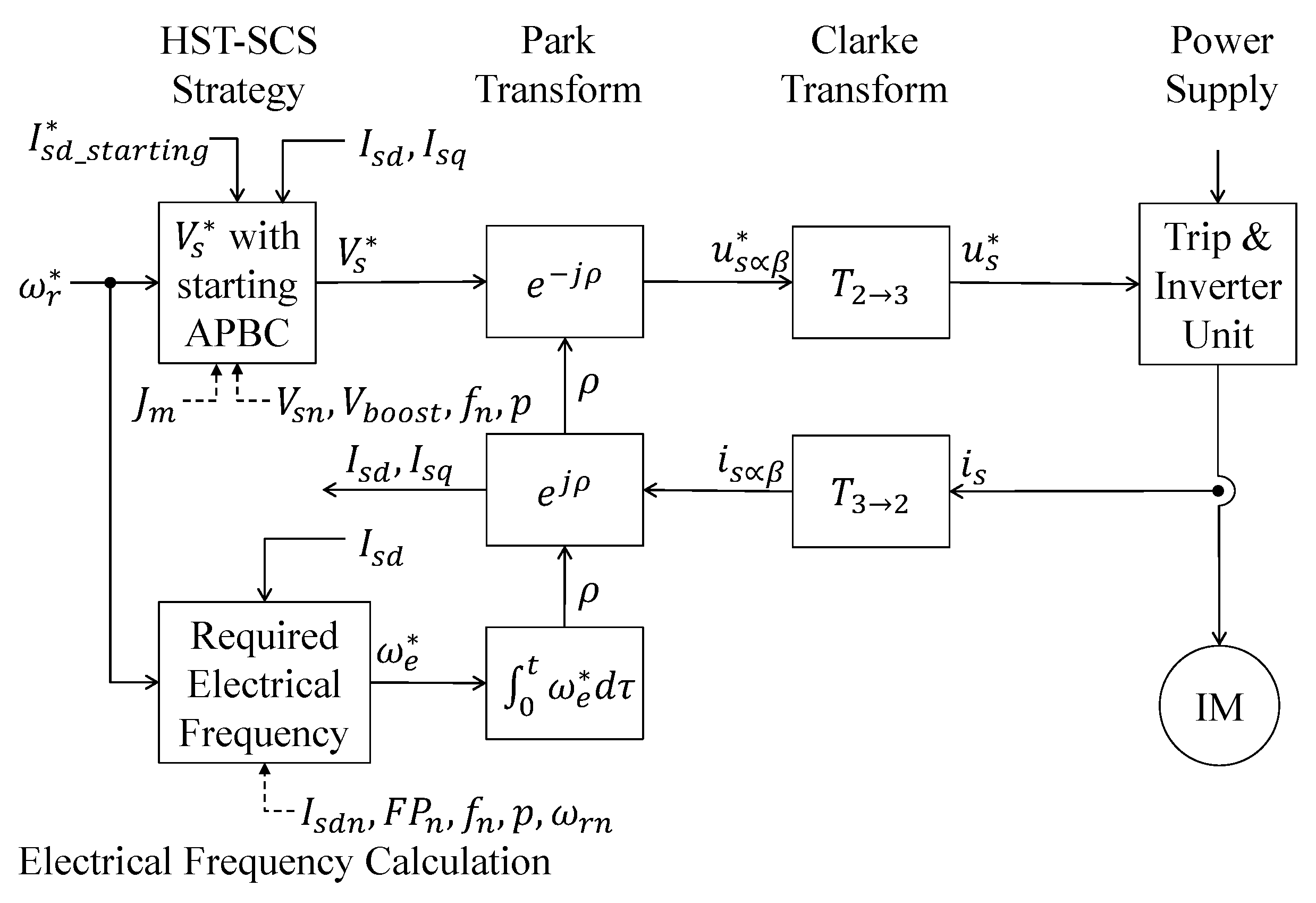
2.3. Methodology Background

The HST-SCS relies on the steady-state IM equivalent circuit per phase. Here, on the one hand, it applies the Kirchhoff’s stator voltage law [3,17,21]. Then, it neglects the stator impedance voltage drop, simplifying the obtained equation as follows:

$$u_s^{*}=\stackrel{dropvoltage\approx 0}{\overbrace{R_s{i}_s+j{\omega }_e^{*}{L}_s^{\prime }{i}_s}}+j{\omega }_e^{*}\stackrel{{\Phi }_s}{\overbrace{L_m{i}_m}}\Rightarrow \left|{\Phi }_s\right|\sim \frac{|u_s|}{{\omega }_e^{*}},$$

(4)

where $R_s$ and $L_s^{\prime }$ are the stator resistance and leakage inductance, respectively. $L_m$ is the magnetizing inductance. Moreover, $i_s$ is the stator phase current, $u_s$ is the stator phase voltage, and $i_m$ is the magnetizing phase current. Based on (4), the voltage curves $V_{s1}^{*}$ and $V_{s2}^{*}$ aim to keep a constant stator flux magnitude $|{\Phi }_s|$ for the ranged ${\omega }_e^{*}$.

On the other hand, the voltage curve $V_{s0}^{*}$, does not use the stator flux magnitude dependence $|{\Phi }_s|\sim \frac{V_s}{{\omega }_e^{*}}$ (4), but its dependence on the magnetizing current, $|{\Phi }_s|=L_m\left|i_m\right|$ [17]. After having that $i_m=i_s-i_r$ and replacing the rotor current $i_r$ expression, we have [17]:

$$\begin{array}{c}|{\Phi }_s|=L_m|i_m|=L_m|i_s-\stackrel{i_r}{\overbrace{\frac{j{L}_m}{\frac{R_r}{{\omega }_{slip}}+j{L}_r}{i}_s}}|,\hfill \\ |{\Phi }_s|=L_m|i_s\left(\frac{\frac{R_r}{{\omega }_{slip}}+j{L}_r^{\prime }}{\frac{R_r}{{\omega }_{slip}}+j{L}_r}\right)|,\hfill \end{array}$$

(5)

where $L_r^{\prime }$ is the rotor leakage inductance. Considering this, the HST-SCS aims to keep a constant starting flux magnitude by fixing the stator phase current $i_s$ (5) at the start. As a result, it guarantees a high starting electromagnetic torque capability, as can be seen next, with $K_p$ a proportionality constant [17]:

$$T_{em}=\stackrel{K_p}{\overbrace{3\left(\frac{p}{2}\right){|\frac{j{L}_m}{\frac{R_r}{{\omega }_{slip}}+j{L}_r}|}^2}}{\left|i_s\right|}^2.$$

(6)

Remark 1.

As shown in Figure 1, the proposed HST-SCS keeps a constant starting stator current direct component $I_{sd\_starting}^{*}$ instead of the needed starting stator current $I_{s\_starting}^{*}$. Moreover, it uses a N-APBC to regulate it [16,17].

The following section proposes using a N-MRAC instead of a N-APBC. Furthermore, it directly controls the starting stator current $i_{s\_starting}$.

3. Proposal

In this section, based on the described IM dynamical d-q model [17], this paper extends an MRAC and applies it to HST-SCS for IM.

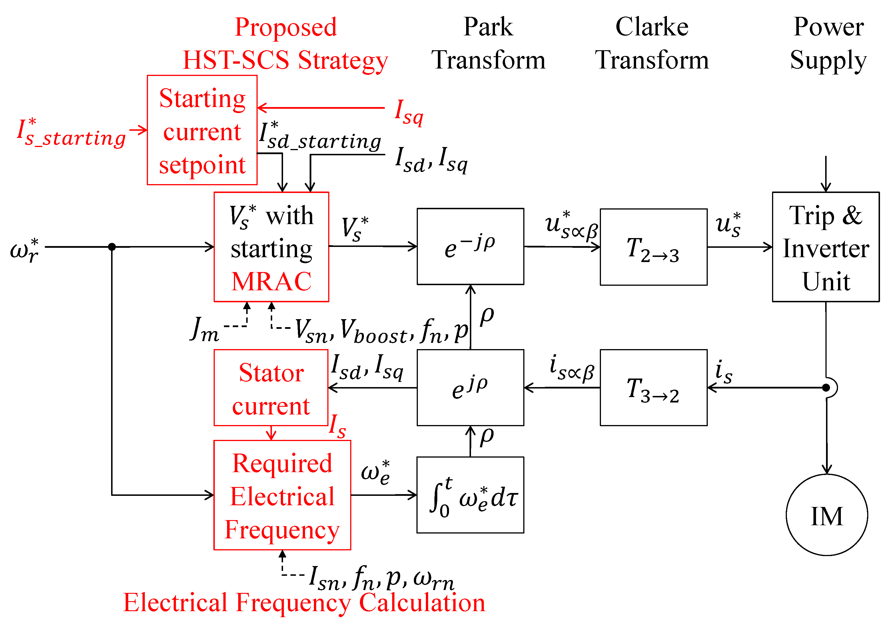
3.1. Proposed N-MRAC for Nonlinear Systems

Let us consider the following class of the nonlinear system:

$$\begin{array}{c}\dot{y}\left(t\right)=\alpha a\left(y\right)+\beta b\left(y\right)u\left(t\right),\hfill \\ \dot{z}\left(t\right)=q(z,y).\hfill \\ \end{array}$$

(7)

Here, the output is $y\left(t\right)\in \Re$, the control input is $u\left(t\right)\in \Re$. The unknown parameters are $\beta \in \Re$ and $\alpha \in {\Re }^{1xm}$. The known nonlinear functions are $b\left(y\right)\in \Re$ and $a\left(y\right)\in {\Re }^m$. It is assumed that it has bounded-input bounded-output (BIBO) internal dynamics $z\left(t\right)\in {\Re }^v$. The dimensions m and v are natural numbers.

The following Theorem 1 extends a direct MRAC [19] to nonlinear systems of the form (7).

Theorem 1.

After considering the desired model reference output $y_m$, and applying the following N-MRAC to the nonlinear system (7), it guarantees that $\underset{t\to \infty }{lim}e\left(t\right)=0$, with $e\left(t\right)=y_m\left(t\right)-y\left(t\right)$:

$$\begin{array}{cc}{\dot{y}}_m\left(t\right)=-A_m{y}_m\left(t\right)+B_m{y}^{*}\left(t\right),\hfill & \hfill \mathrm{model}\mathrm{reference}\\ u\left(t\right)=b{\left(y\right)}^{-l}\theta {\left(t\right)}^T\overline{\Omega \left(t\right)},\hfill & \hfill \mathrm{adaptive}\mathrm{controller}\\ {\theta }^T={\int }_0^t\Gamma e{\overline{\Omega \left(t\right)}}^{T}d\tau ,\mathrm{with}{\theta }^T\left(0\right)=0,\hfill & \hfill \mathrm{adaptive}\mathrm{controller}\mathrm{parameter}\\ {\overline{\Omega \left(t\right)}}^T=100\left[\stackrel{\overline{a\left(y\right)}}{\overbrace{\frac{a\left(y\right)}{a_n}}}\stackrel{\overline{y\left(t\right)}}{\overbrace{\frac{y\left(t\right)}{y_n}}}\stackrel{\overline{y^{*}\left(t\right)}}{\overbrace{\frac{y^{*}\left(t\right)}{y_n^{*}}}}\right],\hfill & \hfill \mathrm{normalized}\mathrm{information}\mathrm{vector}\\ \mathrm{with}\Gamma =\frac{\gamma 100}{1+{100}^2},\hfill & \hfill \mathrm{normalized}\mathrm{fixed}\mathrm{gain}\\ \mathrm{and}{B}_m=S{A}_m.\hfill & \hfill \mathrm{with}\mathrm{S}\mathrm{a}\mathrm{scaling}\mathrm{factor}\end{array}$$

(8)

Here, $y^{*}\left(t\right)$ is the desired trajectory. The normalization factors $a_n$, $y_n$, and $y_n^{*}$ correspond to the maximum operational range of $a\left(y\right)$, $y\left(t\right)$, and $(y^{*}\left(t\right)$, respectively. The normalized information vector considers these factor and has a 100 range. Then, the fixed-gain $\Gamma \in {\Re }^{+}$, having a form $\frac{\gamma \xi }{1+{\xi }^2}$ [19]—Section 5.5, with $\xi =100$ herein due to range of $\overline{\Omega }$, becomes $\frac{\gamma 100}{1+{100}^2}$. It is conformed by the terms $\frac{100}{1+{100}^2}$ for a fast tuning assuring a reasonable operating range and the design parameter $\gamma \in \left[0.1,10\right]$, which allows a fine-tuning adjustment. Moreover, the reference model input $y^{*}$ and output $y_m$ may be expressed in different units of measurement, to which the scaling factor $S\in {\Re }^{+}$ relates.

Appendix A describes the theoretical proof of the proposed N-MRAC. Moreover, the following section includes a design example of the proposed method applied to the HST-SCS of IM.

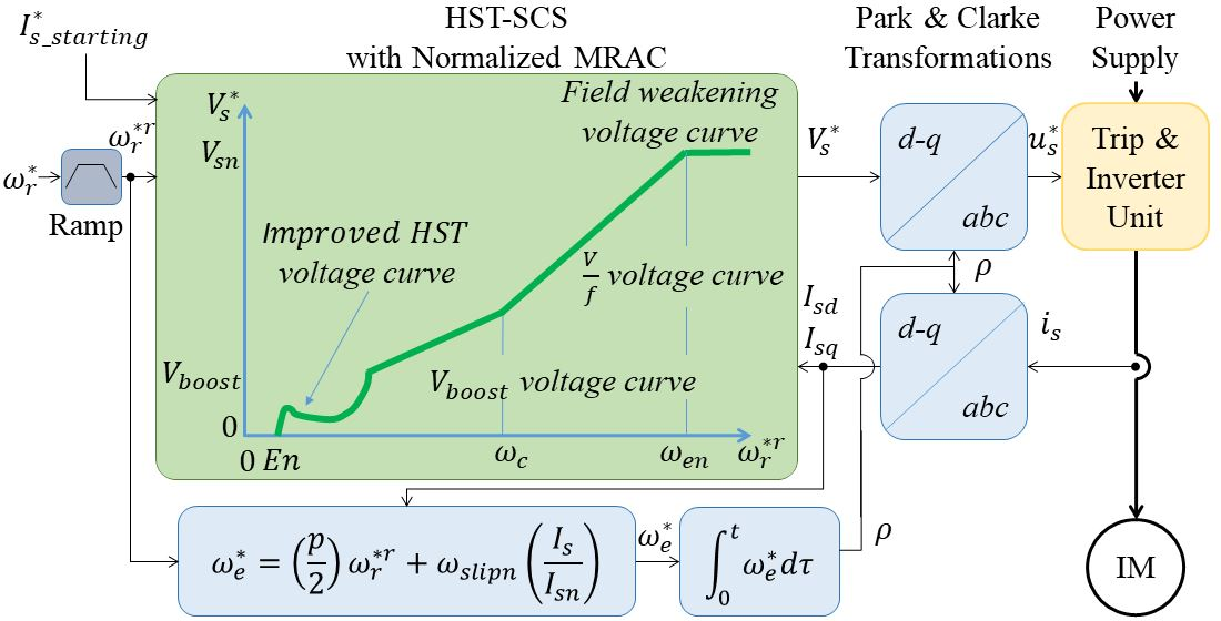
3.2. N-MRAC Applied to HST-SCS for IM

This section uses an N-MRAC as an alternative to the N-APBC proposed in [17] to directly controls the starting stator current $i_{s\_starting}$ as required by (5) and (6).

Figure 2 describes the general block diagram of the proposed HST-SCS, improved after using a N-MRAC and direct control of the stator current $i_s$.

The following subsections describe the details.

3.2.1. Calculus for the Angular Electrical Frequency ${\omega }_e^{*}$

Taken from a proven industry solution [14], here, the slip speed ${\omega }_{slip}$ depends on the rated current per phase $I_{sn}$, and the consumed stator current per phase $I_s$, instead of using the relations given in (1). Hence, the required angular electrical frequency ${\omega }_e^{*}$ computes as follows:

$$\begin{array}{c}{\omega }_e^{*}=\left(\frac{p}{2}\right){\omega }_r^{*}+{\omega }_{slip},\mathrm{with}{\omega }_{slip}={\omega }_{slipn}\frac{I_s}{I_{sn}},\hfill \\ {\omega }_{slipn}={\omega }_{en}-\left(\frac{p}{2}\right){\omega }_{rn},\mathrm{with}{\omega }_{en}=\frac{4\pi f_n}{p}.\hfill \end{array}$$

(9)

The nominal slip ${\omega }_{slipn}$ is calculated as in (1). Please note that $I_{sn}$ and $I_s$ are RMS values used in (9). Hence, the proposal computes $I_s$ as the RMS of the instantaneous vector magnitude $I_{sdq}$ considering it is a sinusoidal signal, and as a function of its instantaneous components as follows:

$$\begin{array}{c}{I}_s=\frac{I_{sdq}}{\sqrt{2}},\mathrm{with}{I}_{sdq}=\sqrt{I_{sd}^2+I_{sq}^2}\hfill \end{array}$$

(10)

The following section describes the required stator voltage amplitude, which follows the same structure as [17] but with a N-MRAC instead of a N-APBC.

3.2.2. Proposed HST-SCS Voltage Amplitude $V_s^{*}$

The proposed HST-SCS considers that IM dynamical d-q model has the form of (7), where the output is $y\left(t\right)=I_{sd}\in \Re$, the control input is $u\left(t\right)=V_{sd}\in \Re$. The unknown parameters are $\beta =\frac{1}{\sigma L_s}$ and $\alpha =\left[A_{1upper}1A_{2upper}\right]\in {\Re }^5$. The known nonlinear functions are $b\left(y\right)=1$ and $a\left(y\right)={\left[I_{sd}{I}_{sq}{\omega }_e^{*}{I}_{sq}\frac{p}{2}{\omega }_r{I}_{sq}\frac{p}{2}{\omega }_r{I}_{sq}\right]}^T\in {\Re }^5$. Moreover, the internal dynamics equals $z\left(t\right)={\left[I_{sq}{\Phi }_{rd}{\Phi }_{rq}{\omega }_r\right]}^T\in {\Re }^4$, defined as follows:

$$q(z,y)=\left[\begin{array}{c}{A}_{1lower}\left[\begin{array}{c}{I}_{sd}\\ I_{sq}\end{array}\right]-{\omega }_e^{*}{I}_{sd}+A_{2lower}\frac{p}{2}{\omega }_r\left[\begin{array}{c}{I}_{sd}\\ I_{sq}\end{array}\right]+\beta V_{sq}\\ C\left[\begin{array}{c}{\Phi }_{rd}\\ {\Phi }_{rq}\end{array}\right]+d\left[\begin{array}{c}{I}_{sd}\\ I_{sq}\end{array}\right]\\ -\frac{b_p}{J}{\omega }_r-\frac{1}{J}\left(\frac{3p{L}_m}{4L_r}\left[\begin{array}{c}{\Phi }_{rd}\\ {\Phi }_{rq}\end{array}\right]\left[\begin{array}{cc}0& 1\\ -1& 0\end{array}\right]\left[\begin{array}{c}{I}_{rd}\\ I_{rq}\end{array}\right]-T_l\right)\end{array}\right].$$

(11)

Here, the stator current direct component $I_{sd}$ is the variable to be controlled via the stator voltage direct component $V_{sd}$. $I_{sq}$ and $V_{sq}$ are the quadrature components of the stator current and the voltage, respectively. ${\Phi }_{rd}$ is the rotor flux direct component, and ${\Phi }_{rq}$ is the rotor flux quadrature component. The rotor angular speed ${\omega }_r$ is assumed to be equal ${\omega }_r^{*}$. Furthermore, the mechanical viscous damping is $b_p$, the motor-load inertia is J, and the load torque is $T_l$. Here, the vector $A_{1upper}\in {\Re }^2$ and $A_{1lower}\in {\Re }^2$ are upper and lower rows of the matrix $A_1$, respectively. The vector $A_{2upper}\in {\Re }^2$ and $A_{2lower}\in {\Re }^2$ are the upper and lower rows of matrix $A_2$, respectively. Moreover, C, d, $A_1$, and $A_2$ are defined as follows [17]:

$$\begin{array}{c}C=\left[\begin{array}{cc}-\frac{R_r}{L_r}& {\omega }_{slip}\\ -{\omega }_{slip}& -\frac{R_r}{L_r}\end{array}\right],d=\frac{R_r{L}_m}{L_r},\\ A_1=\left[\begin{array}{cc}-\frac{R_s^{\prime }}{\sigma L_s}& 0\\ 0& -\frac{R_s^{\prime }}{\sigma L_s}\end{array}\right]-\frac{L_m{R}_r}{\sigma L_s{L}_r^2}d{C}^{-1},A_2=-\frac{L_m{R}_r}{\sigma L_s{L}_r}d\left[\begin{array}{cc}0& 1\\ -1& 0\end{array}\right]C^{-1}.\end{array}$$

(12)

Furthermore, $\sigma$ is the leakage or coupling coefficient, given by $\sigma =1-L_m^2/\left(L_r{L}_s\right)$, $R_s^{\prime }$ is the stator transient resistance, with $R_s^{\prime }=R_s+\left(L_m^2{R}_r\right)/\left(L_r^2\right)$.

After applying the N-MRAC (1) to the IM model, once considering its nonlinear parameters and functions $\alpha$, $\beta$, $a\left(y\right)$, and $b\left(y\right)$, the HST controller conforming the voltage curve $V_{s0}^{*}$ of (2) takes the form:

$$\begin{array}{c}{V}_{s0}=\theta {\left(t\right)}^T\overline{\Omega \left(t\right)},\hfill \\ {\theta }^T={\int }_0^t\Gamma e{\overline{\Omega \left(t\right)}}^{T}d\tau ,\mathrm{with}\Gamma =\frac{\gamma 100}{1+{100}^2},\mathrm{and};{\theta }^T\left(0\right)=0,\hfill \\ \overline{\Omega \left(t\right)}=100{\left[\stackrel{{\overline{\Omega }}_1}{\overbrace{\frac{I_{sd\_starting}^{*}}{I_{sn}}}}\stackrel{{\overline{\Omega }}_2}{\overbrace{\frac{I_{sd}}{I_{sn}}}}\stackrel{{\overline{\Omega }}_3}{\overbrace{\frac{I_{sq}}{I_{sn}}}}\stackrel{{\overline{\Omega }}_4}{\overbrace{\frac{{\omega }_e^{*}{I}_{sq}}{{\omega }_{en}{I}_{sn}}}}\stackrel{{\overline{\Omega }}_5}{\overbrace{\frac{{\omega }_r^{*}{I}_{sd}}{{\omega }_{rn}{I}_{sn}}}}\stackrel{{\overline{\Omega }}_6}{\overbrace{\frac{{\omega }_r^{*}{I}_{sq}}{{\omega }_{rn}{I}_{sn}}}}\right]}^T,\hfill \\ \mathrm{where}e\left(t\right)=I_{sm}\left(t\right)-I_{sn}\left(t\right),\mathrm{with}{\dot{I}}_{sm}\left(t\right)=-A_m{I}_{sm}\left(t\right)+B_m{I}_{s\_starting}^{*},\hfill \\ \mathrm{and}{B}_m=A_m=\frac{5m}{{\tau }_{elect}}.\hfill \end{array}$$

(13)

Here, designer tuning parameters $m\in \left[0.1,10\right]$ and $\gamma \in \left[0.1,10\right]$ to adjust the convergence rate, the electrical time constant ${\tau }_{elect}=\frac{{\tau }_{mech}}{10}$ and the mechanical time constant ${\tau }_{mech}=\frac{1}{2J_m}$ [16,17]. The adaptive controller parameter is $\theta \in {\Re }^6$. The fixed-gain $\Gamma \in {\Re }^{+}$ depends on the design parameter $\gamma \in \left[0.1,10\right]$ to adjust the convergence rate. The following section defines the setpoint $y^{*}\left(t\right)=I_{sd\_starting}^{*}$.

3.2.3. Setpoint of the Starting Stator Current Direct Component $I_{sd\_starting}^{*}$

As the HST-SCS theory [17] relies on the equalities $|{\Phi }_s|\sim |i_s|$ (5) and $T_{em}=K_p{\left|i_s\right|}^2$ (6), the proposed HST-SCS directly controls the starting stator current $I_{s\_starting}^{*}$ establishing the stator current direct component $I_{sd\_starting}^{*}$ based on it, as follows:

$$\begin{array}{c}{I}_{sd\_starting}^{*}=\sqrt{2I_{s\_starting}^2-I_{sq}^2}.\hfill \end{array}$$

(14)

Finally, after applying the proposed N-MRAC to the HST-SCS of IM, the following section describes the experimental results that validate it in practice.

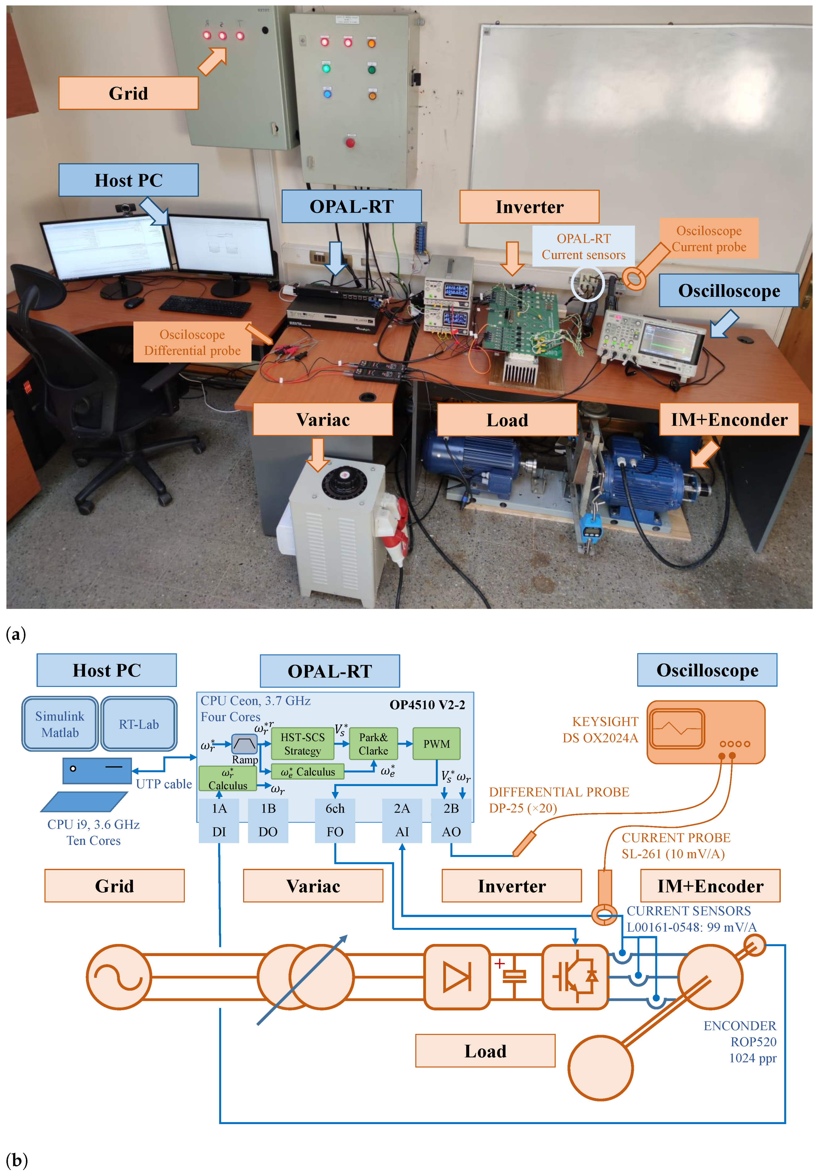
4. Experimental Results

A laboratory test bench allows for conducting experiential testing and obtaining comparative experimental results. It has a real-time simulator controller OPAL-RT 4510 v2, controlling a two-level voltage source inverter unit feeding an IM-load assembly. It inherently uses a bipolar pulse width modulation (PWM) switching at 8 kHz, giving the trip pulses via fiber optic (FO) cables. Simulink version 8.9 and Matlab R2017a running on a Host PC allows building the standard, previous, and proposed HST-SCS, and downloading them to the control platform using the software RT-LAB v2020.2.2.82. Figure 3 shows the test bench used to validate the proposal.

Table 1. Data from the motor nameplate and datasheet.

Symbol	Quantity	Values
$P_n$	rated output power	$7.5$ kW
$V_{sn}$	rated phase voltage	220 V
$I_{sn}$	rated phase current	$15.5$ A
$P{F}_n$	rated power factor	$0.85$
$f_n$	rated electrical frequency	50 Hz
p	poles number	4
${\omega }_{rn}$	rated rotor angular speed	152 rad/s
$J_m$	motor inertia (data-sheet)	0.2 kgm/s${}^2$

depicts the IM main data from the motor nameplate and datasheet. It allows calculating the rated electrical frequency ${\omega }_{en}=\frac{4\pi f}{p}=314.16$ rad/s, the rated electromagnetic torque $T_n=\frac{1000P_n}{{\omega }_{rn}}=49.2$ Nm, and configuring the HT-SCS.

The following section describes the HST-SCS configuration tested.

4.1. HST-SCS Experimental Setup

The experimental setup considers the standard HST-SCS from [14], the previous HST-SCS from [17], and the HST-SCS proposed herein for comparison purposes.

Table 2. Tuning parameters for HST-SCS [17] versus proposed HST-SCS.

Tuning	Standard	Previous	Proposed
Parameter	HST-SCS [14]	HST-SCS [17]	HST-SCS
$V_{boost}$	$40\%V_{sn}$	$40\%V_{sn}$	$40\%V_{sn}$
${\omega }_c$	$50\%{\omega }_{en}$	$50\%{\omega }_{en}$	$50\%{\omega }_{en}$
${\omega }_{min}$	$3\%{\omega }_{en}$	―	―
K	―	$m100J_m$	―
$A_m,B_m$	―	―	$m100J_m$
$\Gamma$	―	$\frac{1}{1+{100}^2}$	$\frac{100}{1+{100}^2}$
$I_{sd}^{*}$	―	$\beta \sqrt{2}{I}_{sn}P{F}_n$	―
$I_s^{*}$	―	―	$I_{sn}$
m	―	6	1
		(malfunctioning below 6)

presents the tuning parameters.

For comparison purposes, with the existing HST-SCS proposed in [17], the following sections repeat the tests made in the manuscript [17]. Hence, the test starts at 0 s and results are shown for over 6 s. Moreover, the applied speed command considers the step wave speed of 200 rpm, 100 rpm, 1500 rpm, 1300, 1100 rpm, at times 1 s, $1.4$ s, $1.7$ s, 4 s, and 5 s, respectively. Furthermore, the following section repeats the tests made in [17] for a starting load torque equals 16% of rated torque and 100% of rated torque.

4.2. Comparative Experimental Results and Discussion

4.2.1. Starting Load Torque equals 16% Tnom

The Prony brake, acting as a load, was set at 21 NM at the rated angular rotor speed of 1455 rpm. It results in a load torque equals $19.6$ Nm (16% of the rated torque) at 200 rpm and 100 rpm, 21 Nm at 1500 rpm, $20.7$ Nm at 1300 rpm, and $20.5$ NM at 1100 rpm. Then, we developed the comparative experiment, having the previously described speed command considered in [17].

Figure 4, Figure 5 and Figure 6 display standard SCS, previous HST-SCS [17], and the proposed HST-SCS experimental results, respectively. Each figure presents the oscilloscope waveforms of the required stator phase voltage amplitude $V_s^{*}$, the rotor angular speed ${\omega }_r$, and the consumed stator phase current $i_{sab}$. As described in Figure 3, the oscilloscope only has four measurement channels, with two of them displaying the signals $V_s^{*}$ and ${\omega }_r$ obtained from the OPAL-RT. The first one has a 200 V per division as indicated in the oscilloscope. The second one has a 1000 rpm per division, although the oscilloscope shows its unit in V.

As shown in Figure 4, Figure 5 and Figure 6, and discussed in [17], the HST-SCS scheme has a peak of 45 A of starting current, lower than the 75 A of standard SCS. This last is characterized by applying the $V_{boost}$ voltage at ${\omega }_{min}$ instead of 0, such as the HST-SCS schemes. Thus, standard SCS has a rotor speed delay of $0.1$ s. The HST-SCS methods start at $1.4$ s, faster than the standard SCS, which begins at $1.5$ s. These are the advantages of the HST-SCS strategies, having a faster speed response and a lower peak current consumption, when compared with standard SCS. Furthermore, the following section shows the additional advantages of starting with a load torque of 100% of the rated torque.

Remark 2.

The obtained results validate in practice the N-MRAC proposed for nonlinear systems and applied to the HST-SCS for IM as an alternative to the N-APBC used in [17].

For all three methods, the voltage curves change smoothly. The adaptive starting voltage curves $V_{s0}^{*}$ switches to the boost voltages curves $V_{s1}^{*}$ around $1.65$ s for the HST-SCS methods, and from $V_{s1}^{*}$ to the $V/f$ voltage curve $V_{s2}^{*}$ around 3 s, including the standard SCS. Moreover, the actual rotor speed follows the required rotor speed with a steady-state accuracy of $1.5$% for speeds over 500 rmp. For lower speeds, the HST-SCS strategies show $1.0$%, lower than the $1.3$% of standard SCS.

Let us now discusses the advantages of the proposed HST-SCS (results are shown in Figure 6) over the previous HST-SCS [17] of Figure 5. As expected, the MRAC current controller shows a smoother response than APBC. Hence, the proposed HST-SCS has a flatter and lower required voltage $V_s^{*}$ and consumed currents $i_a$ and $i_b$. The peak current of the proposed HST-SCS is 36 A, lower than the 40 A of the previous HST-SCS [17].

4.2.2. Starting Load Torque equals 100% Tnom

The Prony brake applied 50 NM with the IM running at the rated angular rotor speed of 1455 rpm. This tuning results in a load torque, equals $49.2$ Nm (the rated torque) at 200 rpm and 100 rpm, $50.6$ Nm at 1500 rpm, $50.4$ Nm at 1300 rpm, and $50.2$ NM at 1100 rpm.

Figure 7 and Figure 8 show the previous HST-SCS [17] and proposed HST-SCS experimental results, respectively. Each figure presents oscilloscope waveforms of a-b line voltage and phase currents, during 100 ms around 4.2, and oscilloscope waveforms of $V_s^{*}$, ${\omega }_r$, and phase currents $i_a$ and $i_b$.

The accomplished experiments verified the results from [16,17] confirming that standard SCS cannot start with rated load torque. Here, Figure 7 and Figure 8 show that, as expected, the IM with HST-SCS started loaded with a nominal torque load achieving the proposed goal. It was done after the HST-SCS applied a DC voltage magnetizing the IM, such as the field-oriented control (FOC). The previous (see Figure 7) and proposed HST-SCS (see Figure 8) have a step stator current reference at $1.4$ s after enabling the VFD.

Moreover, there is no speed and current chattering issues reported in [16], improving the HST-SCS proposed in [16]. It was achieved after all voltage curves changed smoothly, when switching from the voltage $V_{s0}^{*}$ (adaptive starting voltage curve) to the $V_{s1}^{*}$ (boost voltage curve) around $2.3$ s and from the $V_{s1}^{*}$ to the $V_{s2}^{*}$ ($V/f$ voltage curve) around $3.6$ s.

There is a higher speed-response time at the beginning of the simulation. It results from the starting-adaptive controller action, which assures HST capability in this zone. Furthermore, the actual rotor speed follows the required rotor speed with a steady-state accuracy of 2%, as expected for a VFD with the SCS method. It is due to having an open-loop speed control. In contrast to SCS methods, as described in [17], closed-loop speed control FOC or DTC schemes have $0.01$% steady-state speed accuracy, and sensorless strategies have $0.1$%.

Let us now compare the results of the previous HST-SCS from [17], described in Figure 7, and the proposed HST-SCS shown in Figure 8. Again, as in previous subsection, the proposed current N-MRAC shows a smoother $V_s^{*}$ and $I_{s\_starting}$ response than the N-APBC proposed in [17]. The proposal has a slightly lower DC starting current than the previous HST-SCS, 20 A versus 23 A, respectively, between $1.4$ s and 2 s. Moreover, the proposed HST-SCS peak current is 48 A, lower than the previous HST-SCS 56 A. As a result, the proposed HST-SCS has lower integral absolute error (IAE) and integral square input (ISI) indexes than the previous HST-SCS proposed in [17]. These are $38.3$ and $2.613\times {10}^5$ for the proposed HST-SCS and 43 and $2.618\times {10}^5$ for the previous one.

5. Conclusions

This paper proposes a novel N-MRAC for a class of nonlinear systems and its application to the HST-SCS for IM. It started expanding the direct approach of the MRAC strategy, considering a normalized information vector and fixed gains. Appendix A describes its theoretical proof, while experimental results validate, in practice, a design example applied to the HST-SCS of IM.

The proposed N-MRAC is an alternative solution to the N-APBC proposed in [17]. Future work should consider obtaining indirect and combined N-MRAC approaches.

The proposed HST-SCS with N-MRAC assures 100% of the starting electromagnetic torque surpassing the typical 25% of the standard SCS. It does it at the expense of adding a voltage curve at the start, based on an adaptive controller. Moreover, in the proposed method, there is no need for estimators of IM parameters or variables. The proposal only needs information from the IM nameplate and datasheet for its tuning. Hence, it still has a simple control scheme compared to the schemes of FOC and the direct torque control (DTC).

The comparative experiments carried out, considering the N-MRAC and the N-APBC HST-SCS [17], show that both strategies follow the required speed with high starting torque. However, the N-MRAC exhibits lower performance indexes.

References

1. Hannan, M.; Jamal, A.; Mohamed, A.; Hussain, A. Optimization techniques to enhance the performance of induction motor drives: A review. Renew. Sustain. Energy Rev. 2017, 2, 1611–1626. [Google Scholar] [CrossRef]
2. Bose, B.K. Modern Power Electronics and AC Drives; Prentice Hall PTR: Upper Saddle River, NJ, USA, 2002. [Google Scholar]
3. Vas, P. Electrical Machines and Drives: Space Vector Theory Approach; Oxford Clarendon Press: Oxford, UK, 1992. [Google Scholar]
4. Varma, G.H.K.; Barry, V.R.; Kumar Jain, R. A Total-Cross-Tied-Based Dynamic Photovoltaic Array Reconfiguration for Water Pumping System. IEEE Access 2022, 10, 2169–3536. [Google Scholar] [CrossRef]
5. Carbone, L.; Cosso, S.; Kumar, K.; Marchesoni, M.; Passalacqua, M.; Vaccaro, L. Stability Analysis of Open-Loop V/Hz Controlled Asynchronous Machines and Two Novel Mitigation Strategies for Oscillations Suppression. Energies 2022, 15, 1404. [Google Scholar] [CrossRef]
6. Lee, K.; Han, Y. Reactive-Power-Based Robust MTPA Control for V/f Scalar-Controlled Induction Motor Drives. IEEE Trans. Industy Electron. 2022, 69, 169–178. [Google Scholar] [CrossRef]
7. Otkun, O. Scalar speed control of induction motors with difference frequency. J. Polytech. 2020, 238, 267–276. [Google Scholar] [CrossRef]
8. Bala Duranay, Z.; Guldemir, H.; Tuncer, S. Implementation of a V/f Controlled Variable Speed Induction Motor Drive. Int. J. Eng. Technol. 2020, 8, 35–48. [Google Scholar]
9. Tshiloz, K.; Djurovic, S. Scalar controlled induction motor drive speed estimation by adaptive sliding window search of the power signal. Int. J. Electr. Power Energy Syst. 2017, 91, 80–91. [Google Scholar] [CrossRef]
10. Koga, K.; Ueda, R.; Sonoda, T. Constitution of V/f control for reducing the steady-state speed error to zero in induction-motor drive system. IEEE Trans. Industy Appl. 1992, 28, 463–471. [Google Scholar] [CrossRef]
11. Munoz-García, A.; Lipo, T.A.; Novotny, D.W. A new induction motor V/f control method capable of high-performance regulation at low speeds. IEEE Trans. Industy Appl. 1998, 34, 813–821. [Google Scholar] [CrossRef] [Green Version]
12. Wang, C.C.; Fang, C.H. Sensorless scalar-controlled induction motor drives with modified flux observer. IEEE Trans. Energy Convers. 2003, 18, 181–186. [Google Scholar] [CrossRef]
13. Smith, A.; Gadoue, S.; Armstrong, M.; Finch, J. Improved method for the scalar control of induction motor drives. IET Electr. Power Appl. 2003, 7, 487–498. [Google Scholar] [CrossRef] [Green Version]
14. Control Techniques. Commander SE Advanced User Guide; Control Techniques Drives Limited: Hong Kong, China, 2002. [Google Scholar]
15. Zhang, Z.; Bazzi, A.M. Robust Sensorless Scalar Control of Induction Motor Drives with Torque Capability Enhancement at Low Speeds. In Proceedings of the 2019 IEEE International Electric Machines Drives Conference (IEMDC), San Diego, CA, USA, 12–15 May 2019; pp. 1706–1710. [Google Scholar]
16. Travieso-Torres, J.C.; Vilaragut-Llanes, M.; Costa-Montiel, A.; Duarte-Mermoud, M.A.; Aguila-Camacho, N.; Contreras-Jara, C.; Alvarez-Gracia, A. New adaptive high starting torque scalar control scheme for induction motors based on passivity. Energies 2020, 13, 1276. [Google Scholar] [CrossRef] [Green Version]
17. Travieso-Torres, J.C.; Contreras-Jara, C.; Díaz, M.; Aguila-Camacho, N.; Duarte-Mermoud, M.A. New Adaptive Starting Scalar Control Scheme for Induction Motor Variable Speed Drives. IEEE Trans. Energy Convers. 2021, 37, 729–736. [Google Scholar] [CrossRef]
18. Travieso-Torres, J.C.; Duarte-Mermoud, M.A.; Sepúlveda, D.I. Passivity-based control for stabilization, regulation and tracking purposes of a class of nonlinear systems. Int. J. Adapt. Control. Signal Process. 2007, 21, 582–602. [Google Scholar] [CrossRef]
19. Narendra, K.S.; Annaswamy, A.M. Stable Adaptive Systems; Dovers Publications: Mineola, NY, USA, 2005. [Google Scholar]
20. Park, R.H. Two-reaction theory of synchronous machines generalized method of analysis-part I. Trans. Am. Inst. Electr. Eng. 1929, 48, 716–727. [Google Scholar] [CrossRef]
21. Mandic, D.P.; Kanna, S.; Xia, Y.; Moniri, A.; Junyent-Ferre, A.; Constantinides, A.G. A data analytics perspective of power grid analysis-part 1: The Clarke and related transforms. IEEE Signal Process. Mag. 2019, 36, 110–116. [Google Scholar] [CrossRef]
22. O’Rourke, C.J.; Qasim, M.M.; Overlin, M.R.; Kirtley, J.L. A geometric interpretation of reference frames and transformations: dq0, Clarke, and Park. IEEE Trans. Energy Convers. 2019, 34, 2070–2083. [Google Scholar] [CrossRef] [Green Version]
Figure 1. General block diagram of the HST-SCS for IMs, based on [17].
Energies 15 03606 g001
Figure 2. General block diagram of the propose HST-SCS for IMs, remarking the differences in red.
Energies 15 03606 g002
Figure 3. Test bench configuring. (a) Mirror-flipped picture of the test bench. (b) Block diagram of the test bench.
Energies 15 03606 g003
Figure 4. Oscilloscope waveforms of V s * , ω r , and i a and i b , for the standard HST-SCS [14].
Energies 15 03606 g004
Figure 5. Oscilloscope waveforms of V s * , ω r , and i a and i b , for the previous HST-SCS [17].
Energies 15 03606 g005
Figure 6. Oscilloscope waveforms of V s * , ω r , and i a and i b , for the proposed HST-SCS.
Energies 15 03606 g006
Figure 7. Previous HST-SCS [17] experimental results. (a) Oscilloscope waveform of a-b line voltage and phase currents, during 100 ms around 4.2 s. (b) Oscilloscope waveforms of V s * , ω r , and phase currents i a and i b .
Energies 15 03606 g007
Figure 8. Proposed HST-SCS experimental results. (a) Oscilloscope waveform of a-b line voltage and phase currents, during 100 ms around 4.2 s. (b) Oscilloscope waveforms of V s * , ω r , and phase currents i a and i b .
Energies 15 03606 g008