Improving the Maximum Power Extraction from Wind Turbines Using a Second-Generation CRONE Controller

Abstract

Developing precise and robust algorithms that can help in obtaining maximum power yield in a variable speed wind turbine is an important area of research in wind engineering. The present manuscript proposes a technique that utilizes a second-generation CRONE controller for the maximum power tracking technique (MPPT) to maximize power generation in a wind energy conversion system (WECS) based on a double-fed induction generator (DFIG). The authors propose this novel method because the classical controllers cannot provide adequate performance in terms of extracting the maximum energy from variable speed wind turbines when applying a real wind profile and they cannot guarantee the high stability of the WECS. Moreover, this novel controller sufficiently handles problems related to the control effort level. The performance of the second-generation CRONE method was mathematically modeled using MATLAB/Simulink and compared with four other types of MPPT control techniques, which include a proportional-integral linear controller (PI), nonlinear sliding mode controller (SMC), backstepping controller (BS), and fuzzy logic controller (FLC). Two different wind profiles, a step wind profile and a real wind profile, were considered for the comparative study. The response time, dynamic error percentage, and static error percentage were the quantitative parameters compared, and the qualitative parameters included set-point tracking and precision. This test demonstrated the superiority of the second-generation CRONE controller in terms of all of the compared parameters.

1. Introduction

Since the topic of global warming and the global concern for environmental protection have become more prominent, sustainable development has become a concept that consistently accompanies all industrial and economic sectors and influences all new projects. In the context of the electrical energy production sector, governments seek to significantly restrict their dependence on fossil fuel resources, which are known for both their unstable prices and very high greenhouse gas emissions. Electric power operators have been pushed to diversify their energy resources mix, especially with clean and renewable energy from biomass, geothermal energy, solar energy, and wind power sources, which are a consequence of solar energy [1,2].

Recently, this trend has been reinforced by ecological considerations. Indeed, the huge consumption of traditional fossil energy sources leads to serious environmental damage. Therefore, the majority of countries in the world are now involved in the fight against climate change. As far as renewable energies are concerned, there are three main families: thermal (geothermal, solar thermal, etc.), electromagnetic (photovoltaic modules), or mechanical (wind and swell waves) [3]. In particular, wind energy can be used for pumping water after its conversion into mechanical energy or it can be converted into electrical energy through appropriate generators [4]. This second type of conversion has developed considerably all over the world, both through industrial and domestic installations in connection with the electrical power distribution grid [4,5].

Four zones dominate the operation of a wind energy system (Figure 1). The first zone (Zone I) is marked by a low wind velocity that cannot turn the wind turbine to deliver electrical energy. In the second zone (Zone II), the wind turbine system must be controlled to raise the supplied power adequately with changes in wind velocity (by way of MPPT algorithms), and the pitch angle of the blades is maintained at its minimal value. In the third zone (Zone III), while the wind velocity exceeds the nominal optimal value, the blades’ pitch angle must be controlled to ensure the provided power is kept at its desired value. Finally, in Zone IV, the speed of the wind is higher and not suitable, as it can destroy the wind turbine system. Hence, emergency installation devices stop the wind turbine immediately to protect it against eventual damages [5,6].

There are two types of wind energy generators (WEGs): fixed speed WEGs and variable speed WEGs [7,8]. However, the second type offers a wide range operation in terms of wind speed, improved overall efficiency, and higher power-capturing capabilities. Therefore, variable speed WEGs are more advantageous than WEGs with fixed speeds [4].

Nowadays, DFIGs based on variable speed wind turbine systems are the most widely used technology in onshore and offshore wind farms [9,10]. Their key advantage, which is not the only one, is their possession of three-phase static converters, which are dimensioned for a part of the nominal energy of the DFIG [11]. This effect makes DFIGs economical profitable compared to other existing electromechanical conversion solutions (permanent magnet synchronous machines (PMSGs), for example) [12]. Indeed, DFIGs operate at a speed range of ±30% of the speed of synchronization, thus ensuring the minimization of the dimensioning of static converters, as they are linked between the DFIG rotor winding and the electric distribution grid [3].

A wind energy system is considered highly non-linear and characterized by huge and sudden wind speed variations, so the utilization of an MPPT controller is important to order to optimize the generator speed and output power measurements to maximize output power regardless of wind speed [5,6]. The controller allows the maximum MPPT power point to be reached and tracked at all wind speeds [7,8].

There are several maximum power point tracking (MPPT) controls for extracting the maximum amount of energy from wind turbine systems in the literature. In addition, the efficiency and performance of wind turbine systems depend on the efficiency of the used maximum power point tracking (MPPT) control technique [7]. Each MPPT technique can be characterized according to the following criteria: speed of convergence, required sensors, complexity, cost, simplicity of implementation, and other criteria. Therefore, in several research papers [13,14], researchers have sufficiently discussed various MPPT algorithms. Generally, there are two types of MPPT methods. The first category is designated as the direct method and includes the optimum relation-based MPPT (ORB), the hill-climbing search (HCS) (or perturb and observe) and incremental conductance (INC). The second category, on the other hand, is known as indirect control and refers to techniques such as power signal feedback (PSF), optimal torque control (OTC), and tip speed ratio (TSR) [15,16].

The ORB-based MPPT method requires a perfect relationship between speed, wind turbine power output, converter DC voltage, current, and power. The lack of a sensor and fast tracking are the key advantages of this algorithm [17]. However, this technique demands characteristic curves in order to understand the turbine power and converter DC current at different wind speed values. Therefore, the maximum power point can be tracked by observing the optimum current curve [18].

The HCS is an unreliable and a resilient technique which requires previous wind turbine characteristics. For a given function, this algorithm provides the local maximum point. The main drawback of this technique is the likelihood of identifying the wrong direction to reach the most significant power point under a sudden change of the wind direction [19].

INC requires sensors and wind turbine and generator parameters. Therefore, the main advantages of this technique are cost reductions and improvements in terms of reliability [20]. The power-speed slope allows for the determination of the operating point of the MPPT. However, the drawback of this algorithm is its instability with respect to variations in turbine inertia under a variable speed wind profile [21].

The PSF approach uses a power control loop which integrates inputs regarding the wind turbine maximum power curve [22]. While the TSR controller is characterized by its simplicity of design, the drawback of this method is its need for an optimal power coefficient and an optimal tip-speed ratio [23].

The OTC-based MPPT method implies changing the generator torque according to the relevant power reference torque at all wind speed values [24]. This technique is characterized by its simplicity, fast response, and efficiency. Moreover, wind speed changes are not reflected in the reference signal because of the absence of direct wind speed measurements [13].

Another intelligent method for determining the maximum power point is called the artificial neural network (ANN). This technique involves taking different input variables and handling them to obtain the maximum power [25]. For this controller, there is no condition with respect to the assigned nodes numbers and all neural networks include an input layer, an output layer, and a hidden layer. This controller is a reliable alternative to conventional MPPT controllers. However, the disadvantages of ANNs include the empirical nature of the development of the model, increased computing loads, their black box structure, and over-fitting issues. In addition, this method demands the use of a look-up table containing predefined data [26].

In [6], the researchers proposed a fuzzy regulator to enhance the performance of the predictive torque control model. Indeed, the variable-weight model known as predictive torque control was applied to a real wind turbine to extract the maximum power. On the other hand, in [27], a stochastic model predictive yaw control (SMPYC) strategy based on intelligent scenarios generation (ISG) was proposed to improve in the energy capture efficiency of a wind turbine. The ISG technique is used to generate scenarios that characterize its application, then the yaw action is optimized via the proposed scenario-based SMPYC and can be performed to enhance the power capture efficiency of wind turbines.

Likewise, several research works have focused on linear control methods such as H∞ [28], and other researchers have compared linear and non-linear controllers. The researchers in [29] used the CRONE (French abbreviation: “Commande Robuste d’Ordre Non Entier”) controller for the MPPT technique in the context of a WECS-based on hybrid excitation synchronous generator (HESG). But this strategy is used only for linear systems, hence non-linear systems must be linearized. The CRONE controller is widely used in the field of vehicles, as it demonstrates a high level of robustness for this type of application [30,31].

According to what exists in the literature, this research work can be considered the first work that uses the CRONE controller for the MPPT technique for a WECS based on a DFIG. It is also the first work that validates and compares the results of this controller with four other MPPT techniques applied to the same system. Generally, few works based on the CRONE technique are used in the field of wind energy conversion systems to extract the maximum wind power [29].

The objective of this paper was to elaborate on MPPT-based control via the controlling of the mechanical speed of a wind turbine. Indeed, the second-generation CRONE controller is proposed to ensure the follow up of the set-point, which is a function of the wind velocity, and to ensure system stability. This new control strategy for a DFIG-based WECS is compared to four other existing controllers, which are, respectively, a proportional-integral (PI) linear controller, a nonlinear sliding mode controller (SMC), a backstepping (BS) controller, and a fuzzy logic controller. Hence, the results of the analysis show that the CRONE controller designed in this study provides great precision, good reference tracking, and a high level of efficiency enhancement compared to the other controllers used in this paper. Moreover, this method allowed the wind turbine aerodynamic system to work with good stability. This controller significantly reduced the response time of the system.

This research paper will be organized as follows: the second section, following the introduction, is reserved for the mathematical modeling of the wind turbine and its mechanical parts; the third section details the proposed control method and four other strategies; a discussion of the obtained results and a comparative study are provided in Section 4; and, finally, the conclusion and some additional perspectives are summarized in Section 5.

2. Mathematical Model of the Wind Energy Conversion System

The wind power that passes through a surface S can be expressed as [1]:

$$P_V=\frac{\rho S{V}^3}{2}$$

(1)

where V is the wind velocity (m/s), ρ is equal to 1.225 kg/m³, which is the air density and R is the radius of the turbine blade.

The wind turbine can capture only a fraction of the wind energy and the captured aerodynamic power of the turbine can be formulated as [1,2]:

$$P_t=C_p{P}_V=\frac{1}{2}\rho \pi R^2{V}^3{C}_p\left(\lambda ,\beta \right)$$

(2)

C_p is the power coefficient representing the wind turbine’s aerodynamic efficiency.

The blade pitch angle β and the tip speed ratio λ are involved in the expression of C_p.

The tip-speed ratio is defined as [13]:

$$\lambda =\frac{{\mathsf{\Omega }}_{t}R}{V}$$

(3)

with ${\mathsf{\Omega }}_t$ (rad/s) being the turbine angular speed on the low-speed side of the turbine gearbox.

In this paper, $C_p$ is written in the following form [13]:

$$C_p\left(\lambda , \beta \right)=0.5\left(\frac{116}{\lambda i}-0.4\beta -5\right)exp\left(\frac{-21}{\lambda i}\right)+0.0068\lambda$$

(4)

with $\frac{1}{\lambda i}$=$\frac{1}{\lambda +0.08\beta }-\frac{0.035}{{\beta }^3+1}$.

The aerodynamic torque of the turbine is defined as [1]:

$$C_t=\frac{P_t}{{\mathsf{\Omega }}_t}=\frac{1}{2}\rho \pi R^3{V}^3{C}_c\left(\lambda ,\beta \right)$$

(5)

where C_c represents the torque coefficient [1]:

$$C_c=\frac{C_p}{\lambda }$$

(6)

Figure 2 reflects the evolution of the power coefficient C_p in its relationship with the tip-speed ratio and blade pitch angles β.

From Figure 2, it can be noted that for every blade pitch angle β there is a specific optimal tip-speed ratio λ that ensures the maximum value of the coefficient C_p. In addition, the power coefficient achieves its highest value (C_pmax = 0.48) when β = 0, then the tip-speed ratio becomes constant at its optimal specific value (λ_opt = 8.1). Therefore, it is possible to elaborate a control law that allows for the capturing of the maximum wind power whatever the wind speed until the maximum generator power is reached. This target can be achieved by using the MPPT. By other means, to set λ at its specific optimum desired value and to maximize the generated wind turbine power, the speed Ω_t must be linearly varied with the wind speed V changes. In this case, the optimal rotational speed Ω_t^opt can be given for the maximum mechanical transmission of the wind turbine by the following expression [18]:

$${\mathsf{\Omega }}_t^{opt}=\frac{{\lambda }_{opt}}{R}$$

(7)

Equation (2) can be written as [16]:

$$P_t^{opt}=\frac{1}{2}\rho \pi R^2{V}^3{C}_p^{max}\left({\lambda }_{opt},{\beta }_{opt}\right)$$

(8)

Equation (8) shows that a small variation in the wind speed results in a large variation in the generated power P_t.

The gearbox adapts the turbine speed (slow shaft) to the generator speed (fast shaft). The elasticity and friction of the gearbox are neglected. Thus, the energy losses are considered to be zero. The mathematical model of the gearbox is presented as [3,16]:

$${\mathsf{\Omega }}_t=\frac{{\mathsf{\Omega }}_g}{G}$$

(9)

where ${\mathsf{\Omega }}_t$ is the turbine speed, ${\mathsf{\Omega }}_g$ is the generator speed, and G is gearbox gain.

The proposed mechanical model, in this work, considers the total inertia $J$ as the sum of the transferred turbine inertia $J_t$ and the inertia of the generator $J_g$ [16]:

$$J=\frac{J_t}{G^2}+J_g$$

(10)

The equations of both the electromagnetic and mechanical torques are written as follows [15]:

$$\frac{d{\mathsf{\Omega }}_g}{dt}=C_{mec}=C_g-C_{em}-C_f$$

(11)

Therefore, the mechanical speed evolution ${\mathsf{\Omega }}_g$ depends on the mechanical torque applied to the rotor $C_g$, the electromagnetic torque $C_{em}$, and the viscous friction torque $C_f$ given by the relation [32]:

$$C_f=F_v{\mathsf{\Omega }}_g$$

(12)

where F_v is the friction coefficient.

Figure 3 presents the aerodynamic model of the studied wind turbine system. This scheme indicates that the rotation speed of the generator ${\mathsf{\Omega }}_g$ and the turbine speed can be controlled by acting on the electromagnetic torque $C_{em}$ of the generator.

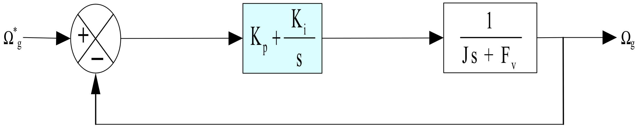
3. MPPT Strategy with Speed Control

The control algorithms strategy consists of adjusting the generator’s electromagnetic torque to push the mechanical speed to pursue a reference value. The latter will maximize the extracted power of the turbine [13]. Consequently, the speed of the generator must be controlled. For a given operating point (fixed wind speed), the maximum aerodynamic mechanical power can be reached if the wind system is operating at its maximum value of the power coefficient C_p [18]. Moreover, this can be realized when the tip-speed ratio (λ) achieves its desired optimum value λ_opt. Therefore, the desired speed of the generator ${\mathsf{\Omega }}_g^{*}$ is obtained by using Equations (3), (7) and (9) as follows:

$${\mathsf{\Omega }}_g^{*}=G\frac{{\lambda }_{opt}}{R} V$$

(13)

The overall scheme of the proposed MPPT strategy is shown in Figure 4, where the electromagnetic torque reference $C_g^{*}$, which is used to control the speed of the DFIG rotor, is obtained at the output of the speed controller.

3.1. CRONE Controller

The CRONE strategy is a frequency-domain method for robust control. Indeed, the corrected open loop’s transfer function for this approach is characterized by a non-integer order, namely a fractional order [33].

The CRONE control system design (CSD) approach was presented and designed in the 1980s [33,34,35,36,37,38] (see Figure 5). It was designed based on common unity feedback configuration systems.

This control strategy has three generations:

▪

The first generation of CRONE is used in cases where only the gain variations of the studied nominal model are to be controlled.

▪

The second CRONE control strategy is used when there are both variations for the gain and the transitional frequencies of the controlled model.

▪

The third generation CRONE is used when there are several uncertain parameters other than gain and phase [33,37].

For these three generations, the transfer function of the open-loop or controller is developed by using integro-differential equations of fractional order [39,40].

3.1.1. The First-Generation CRONE Method

The first CRONE CSD generation strategy is based on a constant-phase controller and centers on the specific desired open-loop gain crossover frequency ω_cg, calculated via a band-limited real fractional differentiator [39,40,41].

$$C(s)=C_0{\left(\frac{\frac{s}{{\omega }_l}+1}{\frac{s}{{\omega }_h}+1}\right)}^n$$

(14)

with C₀, ω_l, ω_h, and n being real parameters.

The constant-phase controller guarantees the robustness of the phase margin when the phase plant remains constant around the frequency ω_cg in the case of plant perturbations leading to gain variations around ω_cg only.

The CRONE controller has to embed an order-n_F low-pass filter and an order-n_I band-limited integrator to manipulate the steady-state error and the effort level of the control. Hence, the 1st generation CRONE controller is presented as follows [38,41]:

$$C_F(s)=C_0\frac{1}{{\left(1+\frac{s}{{\omega }_F}\right)}^{n_F{}^{\prime }}}{\left(\frac{\frac{s}{{\omega }_l}+1}{\frac{s}{{\omega }_h}+1}\right)}^n{\left(1+\frac{{\omega }_I}{s}\right)}^{n_I}$$

(15)

with ω_I, ω_F being positive reals and n_I, n_F being positive integers.

This controller can be defined as a PI^n_IDⁿF^n_F controller. Hence, with a rational approximation of the fractional element of (15) an implementable version of this controller can be defined. It is achieved using the recursive distribution of real-valued poles and zeros [41]:

$${\displaystyle \prod _{i=1}^N\left(\frac{\frac{s}{{\omega }_i^{\prime }}+1}{\frac{s}{{\omega }_i}+1}\right)}$$

(16)

where ${\omega }_i^{\prime }$ and ω are reals and N is a positive integer.

Moreover [39,41]:

$$\begin{array}{l}\eta =\frac{{\omega }_{i+1}^{\prime }}{{\omega }_i^{\prime }};\alpha =\frac{{\omega }_i}{{\omega }_i^{\prime }};\log (\alpha )=n\log (\alpha \eta );\alpha \eta =\left(\frac{{\omega }_h}{{\omega }_l}\right)\\ \end{array}$$

(17)

To ensure the robustness of the phase margin, the ω_cg must be located in the frequency range where the phase of the plant remains constant. However, only the variation of the gain-like plant may happen [37,38,39,40,41].

When the previous condition is not verified, the second-generation CRONE CSD strategy should be used [41].

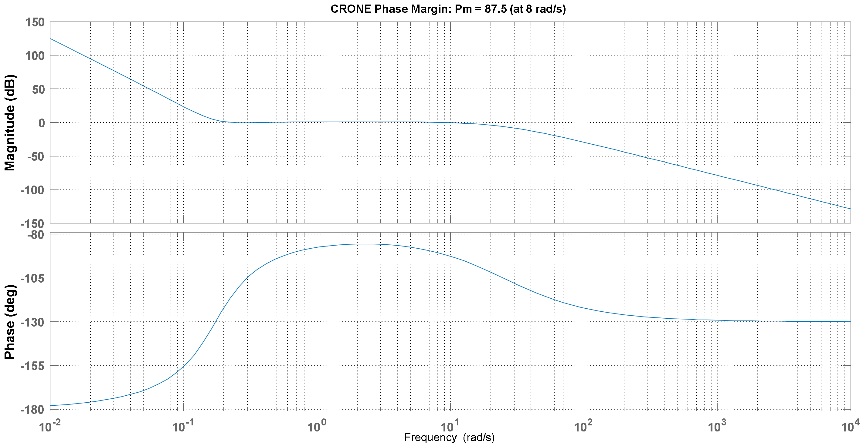
3.1.2. The Second-Generation CRONE Method

For some systems, and due to problems related to controlling the effort-level, it is very difficult, or even impossible, to take an ω_cg from the frequency range where the phase of the plant remains constant. However, Bode [42] indicated that a robust controller can allow the open-loop transfer function to be determined by a fixed phase in a practical and useful band. The achievement of Bode was “The design of single loop stable amplifiers” which have variable tube gains [40,41,42].

Consequently, the second-generation CRONE method considers the open-loop transfer function in the vicinity of ω_cg as a transfer function of a fractional integrator [41].

$$\beta (s)={\left(\frac{{\omega }_{cg}}{s}\right)}^n$$

(18)

With n being a positive integer.

Depending on gain variations, the vertical template, which is the vertical sliding of the vertical Nichols locus, is permitted to have [35,41]:

• A constant phase margin,
• A resonant peak Mr,
• A modulus margin, which is the minimal distance between the critical point and the open-loop Nyquist locus,
• The damping ratio of the closed-loop system.

By using integer orders n_l and n_h, and to enable the controller to process robustness, accuracy, and control effort problems, the nominal open-loop transfer function is given as follows [38,39,40,41]:

$${\beta }_0(s)=K{\left(1+\frac{s}{{\omega }_h}\right)}^{-n_h}{\left(\frac{1+\frac{s}{{\omega }_h}}{\frac{s}{{\omega }_l}}\right)}^n{\left(\frac{1+\frac{s}{{\omega }_l}}{\frac{s}{{\omega }_l}}\right)}^{n_l}$$

(19)

where:

n_l is an integer order and it must be set to adjust the accuracy supplied by the control system;

n_h is an integer order and it must be set to have a proper or bi-proper controller.

The ratio of the nominal open-loop and the plant transfer function presents the fractional controller C_F(s) [41]:

$$C_F(s)=\frac{{\beta }_0(s)}{G_0(s)}$$

(20)

In summary, the rational transfer function C_R(s) (i.e., with integer orders) can be presented by substituting the fractional element of (20) using the rational approximation (16).

3.1.3. The Third Generation CRONE Method

There are cases where the vertical Nichols locus does not slide on itself. These cases are more delicate and general than the problem of gain-like plant variations [33].

It is more suitable to take a Nichols locus, which is always determined as a straight-line segment around the specific frequency ω_cg, for the plant nominal parametric state, but with any space direction. Hence, the open-loop transfer function in this case is determined by the real element with regard to the imaginary “i” of a fractional-order complex integrator transfer function [33,41]:

$$\beta (s)={\mathrm{Re}}_{/i}{\left(\frac{{\omega }_{cg}}{s}\right)}^n$$

(21)

with s = σ + jω ∈ C_j and n = a + ib ∈ C_j.

Where:

• “a” is the real order which determines the Nichols locus phase placement is called the generalized template.
• “b” is the imaginary order which determines the Nichols locus angle with respect to the vertical.

The concept of the third generation CRONE method is to try to optimize the parameters of the nominal open-loop transfer function β₀(s), which embeds a band-limited complex fractional-order integration [41].

$${\beta }_0(s)={\beta }_m(s).{\beta }_l(s).{\beta }_h(s)$$

(22)

where [39]:

$${\beta }_l(s)=C_l{\left(\frac{{\omega }_{-N^{-}}}{s}+1\right)}^{n_l}$$

(23)

$${\beta }_h(s)=C_h{\left(\frac{s}{{\omega }_{N^{+}}}+1\right)}^{-n_h}$$

(24)

$${\beta }_m(s)={{\displaystyle \prod _{k=-N^{-}}^{N^{+}}{C}_k^{sign(b_k)}\left({\alpha }_k\frac{\frac{s}{{\omega }_{k+1}}+1}{\frac{s}{{\omega }_k}+1}\right)}}^{a_k}{\left[{\mathrm{Re}}_{/i}{\left\{{\alpha }_k\frac{\frac{s}{{\omega }_{k+1}}+1}{\frac{s}{{\omega }_k}+1}\right\}}^{i{b}_k}\right]}^{-q_{k}sign(b_k)}$$

(25)

with a_k, b_k, ω_k, ω_k+1, ω_r, α_k, C_k, C_h and C_l ∈$ℝ$ and N⁺, N⁻ and q_k ∈$\mathbb{N}$.

The gains, “C”, were taken in such a way that ωr has to be the nominal closed-loop resonant frequency. Then, the optimization is simplified considerably by the open-loop transfer function parameterization of complex fractional orders [39,40,41].

In the process of optimization, a complex order can be considered as a large set of parameters that are included in common rational controllers. Consequently, the fractional controller CF(s) is presented by its frequency response as follows [41]:

$$C_F(j\omega )=\frac{{\beta }_0(j\omega )}{G_0(j\omega )}$$

(26)

The rational transfer function CR(s) parameters with a predefined low-order structure are adjusted to accommodate the desired frequency response C_F(jω). This goal can be achieved by using any frequency domain system identification approach [41].

The advantages of this approach include the fact that despite the complexity of the control system problem, a controller order reduced value, which is usually around 6, can be used [35,41].

3.1.4. CRONE Method Design for Wind Turbine MPPT

Depending on the CRONE generation, the non-integer, real, or complex order will be obtained to allow the definition of the open-loop transfer function, which is optimal in terms of speed, overshoot, and accuracy with some parameters [35]. Based on the WECS model specifications, the second CRONE generation was used in this research work [41].

The CRONE control approach is based on the determination of the open loop’s transfer function β(s) (27) for the nominal state of the plant G(s). This function β(s) must guarantee, around the desired bandwidth ω₀ = 8 rad/s, a very good phase margin, i.e., greater than 80° [39].

The angular velocity’s closed-loop’s settling is fixed at 8 s, which is technically logic for the WECS based on a DFIG. Furthermore, the rotor current settling is set at 0.01 s to guarantee that the inner current’s loop must be at least ten times faster than the outer velocity loop. To ensure a ratio of 10, which is usual, between the two loops, the velocity loop’s bandwidth is set at 8 rad/s, taking into account that the rotor current loop’s bandwidth is about 310 rad/s [41].

Thus, the open loop’s transfer function β(s) (see Figure 5) is determinate by the following equations [41]:

$$\beta (s)=K_{CRONE}(s).G(s)$$

(27)

where G(s) is the uncertain plant model [3,18]:

$$G(s)=\frac{\mathrm{\Omega }}{C_m-C_{em}}=\frac{1}{J.s-F_V}$$

(28)

where J is the moment of the inertia and Fv is the coefficient of the viscous friction.

The open-loop transfer function can be written as follows [29,41]:

$$\beta (s)=K_u{\left(1+\frac{s}{{\omega }_h}\right)}^{-n_h}{\left(\frac{1+\frac{s}{{\omega }_h}}{\frac{s}{{\omega }_l}}\right)}^n{\left(\frac{1+\frac{s}{{\omega }_l}}{\frac{s}{{\omega }_l}}\right)}^{n_l}$$

(29)

$$K_u={\left(\frac{{\omega }_0}{{\omega }_l}\right)}^{n_l}.{\left(1+{\left(\frac{{\omega }_0}{{\omega }_l}\right)}^2\right)}^{\left(\frac{n-n_l}{2}\right)}.{\left(1+{\left(\frac{{\omega }_0}{{\omega }_h}\right)}^2\right)}^{{}^{\left(\frac{n_h-n_l}{2}\right)}}$$

(30)

with:

${\omega }_l=\frac{{\omega }_0}{10\sqrt{a}}$; ${\omega }_h={\omega }_{0}10\sqrt{a}$; $a=\Delta {\beta }^{\frac{1}{n}}$ and $n=\frac{180-M\varphi }{90}$

Where:

K_CRONE(s): the CRONE controller

Ku: the constant which ensures the unity gain at the specific desired frequency ω₀.

ω_h, ω_l: the high and low transitional frequencies.

n_h, n_l,, and n: The order at high frequency, the order at the low frequency, and the order around the crossover frequency, respectively.

Δβ: The variation of the gain in the open-loop.

Mϕ: The desired phase margin in degrees.

In this work, Mϕ was set to 85°. n_h and n_l were taken to be equal to 1.5 and 2, respectively, for the purpose of limiting the input sensitivity and guaranteeing a zero steady-state error, respectively.

The CRONE toolbox [43] is used to synthesize the CRONE controller as follows:

$$K_{CRONE}=\frac{2.67s^2+0.517s+0.08}{s^3+25.2s^2}$$

(31)

Figure 6 proves that a good phase margin of 87.2° is reached at around 8 rad/s, which is the crossover frequency.

3.2. PI Controller

The loop of speed control described in Figure 7 is designed from the equation of the dynamics of the rotating bodies [14,44].

The closed-loop transfer function is written as follows [44]:

$$\frac{{\mathsf{\Omega }}_{g\left(s\right)}}{{\mathsf{\Omega }}_{g^{*}\left(s\right)}}=\frac{2\xi .{\omega }_n.s+{\omega }_n^2}{s^2+2\xi .{\omega }_n.s+{\omega }_n^2}=\frac{\frac{K_i+K_p.S}{J}}{s^2+\frac{K_p+F_v}{J}.s+\frac{K_i}{J}}$$

(32)

Both of the parameters $K_p$ and $K_i$, of the proportional-integral controller, are given by the following expressions [44]:

$$\left\{\begin{array}{c}{K}_p=2\xi .{\omega }_n.J-F_V\\ K_i=J.{\omega }_n^2\end{array}\right.$$

(33)

3.3. Nonlinear Backstepping (BS) Controller

The backstepping methodology can be presented as a technique for organizing a studied system into several cascading sub-systems. The execution of the design methodology on a general level results in the establishment of a control law via feedback which is systematically associated with a Lyapunov function or the equivalent. A control law method stabilizing the studied system is derived from a Lyapunov function to prove the stability [45]. The important properties of the overall stability of each subsystem are obtained by defining a stabilizing function at each stage of the representation of the model in cascade subsystems. One of the greatest advantages engendered by the backstepping algorithm method is the of maintaining of the features of the initial system in the obtained control laws [46]. This is the great asset of the backstepping control, especially when compared to other control methods [47]. The backstepping control method is implemented to create a control law using Equation (11) in order to force the system to follow the required trajectory.

The tracking error is defined as [45]:

$$e\left({\mathsf{\Omega }}_g\right)={\mathsf{\Omega }}_g^{*}-{\mathsf{\Omega }}_g$$

(34)

The derivative of Equation (34) is expressed as [46]:

$$\dot{e}\left({\mathsf{\Omega }}_g\right)=\dot{{\mathsf{\Omega }}_g^{*}}-\dot{{\mathsf{\Omega }}_g}$$

(35)

Considering the following Lyapunov function [45,46]:

$$v\left(e\right)=\frac{1}{2}e{\left({\mathsf{\Omega }}_g\right)}^2$$

(36)

The derivative of the Lyapunov function can be written as [45]:

$$\dot{v}\left(e\right)=e\left({\mathsf{\Omega }}_g\right).\dot{e}\left({\mathsf{\Omega }}_g\right)=e\left({\mathsf{\Omega }}_g\right).\left(\dot{{\mathsf{\Omega }}_g^{*}}+\frac{1}{J}\left(C_{em}+f_v.{\mathsf{\Omega }}_g-C_g\right)\right)$$

(37)

The function of the stabilizing control of backstepping is defined by the following equations [45]:

$$C_{em}^{*}=-J.\dot{{\mathsf{\Omega }}_g^{*}}-f_v.{\mathsf{\Omega }}_g+C_g-K_1.e\left({\mathsf{\Omega }}_g\right)$$

(38)

$K_1$ is a specific positive constant [45].

Substituting (38) in (37), the derivative with respect to time can be reformulated as:

$$\dot{v}\left(e\right)=-K_1.e{\left({\mathsf{\Omega }}_g\right)}^2<0$$

(39)

3.4. Sliding Mode Controller (SMC)

The sliding mode control strategy is the combination of a non-linear control method and a variable structure method. Furthermore, the several control structures are created in such a way that the trajectories always converge to a defined adjacent region of the sliding structure which presented the system’s normal behavior [48]. This will slide along the boundaries of the control structures [49]. Moreover, the system motion, as it slides along these boundaries, is named as a sliding mode and the sliding surface is the geometrical locus consisting of the boundaries [48].

To design the command $C_{em}^{*}$, the surface relative degree is set to 1. On the other hand, the sliding surface is determined in the following manner [50]:

$$S\left({\mathsf{\Omega }}_g\right)={\mathsf{\Omega }}_g^{*}-{\mathsf{\Omega }}_g$$

(40)

Choosing the following Lyapunov function [49]:

$$V\left(S\left({\mathsf{\Omega }}_g\right)\right)=\frac{1}{2}S{\left({\mathsf{\Omega }}_g\right)}^2$$

(41)

Its time derivative is [49]:

$$\dot{V}\left(S\left({\mathsf{\Omega }}_g\right)\right)=S\left({\mathsf{\Omega }}_g\right).\dot{S}\left({\mathsf{\Omega }}_g\right)$$

(42)

with: $\dot{S}\left({\mathsf{\Omega }}_g\right)=\dot{{\mathsf{\Omega }}_g^{*}}-\dot{{\mathsf{\Omega }}_g}$.

Substituting Equation (11) in (42), the obtained equation is [49]:

$$\dot{S}\left({\mathsf{\Omega }}_g\right)=\dot{{\mathsf{\Omega }}_g^{*}}+\frac{1}{J}\left(C_{em}+f_v.{\mathsf{\Omega }}_g-C_g\right)$$

(43)

By replacing the expression of $C_{em}$ by the equivalent commands $\left(C_{emeq}+C_{emn}\right)$ in Equation (43), we find:

$$\dot{S}\left({\mathsf{\Omega }}_g\right)=\dot{{\mathsf{\Omega }}_g^{*}}+\frac{1}{J}\left(\left(C_{emeq}+C_{emn}\right)+f_v.{\mathsf{\Omega }}_g-C_g\right)$$

(44)

In the steady-state and during the sliding mode and we obtain: $C_{emn}=0$, $S\left({\mathsf{\Omega }}_g\right)=0,$ and $\dot{S}\left({\mathsf{\Omega }}_g\right)=0$. From the previous equations, we extract the expression of the equivalent command $C_{emeq}$ [49]:

$$C_{emeq}=-J.\dot{{\mathsf{\Omega }}_g^{*}}-f_v.{\mathsf{\Omega }}_g+C_g$$

(45)

Using Equations (45) in (44), the sliding surface derivative can be reformulated as [49,50]:

$$\dot{S}\left({\mathsf{\Omega }}_g\right)=\frac{1}{J}{C}_{emn}$$

(46)

To guarantee the convergence of the Lyapunov function, we take [49]:

$$C_{emn}=-K_2.sign\left(S\left({\mathsf{\Omega }}_g\right)\right)$$

(47)

where $K_2$ is a positive constant.

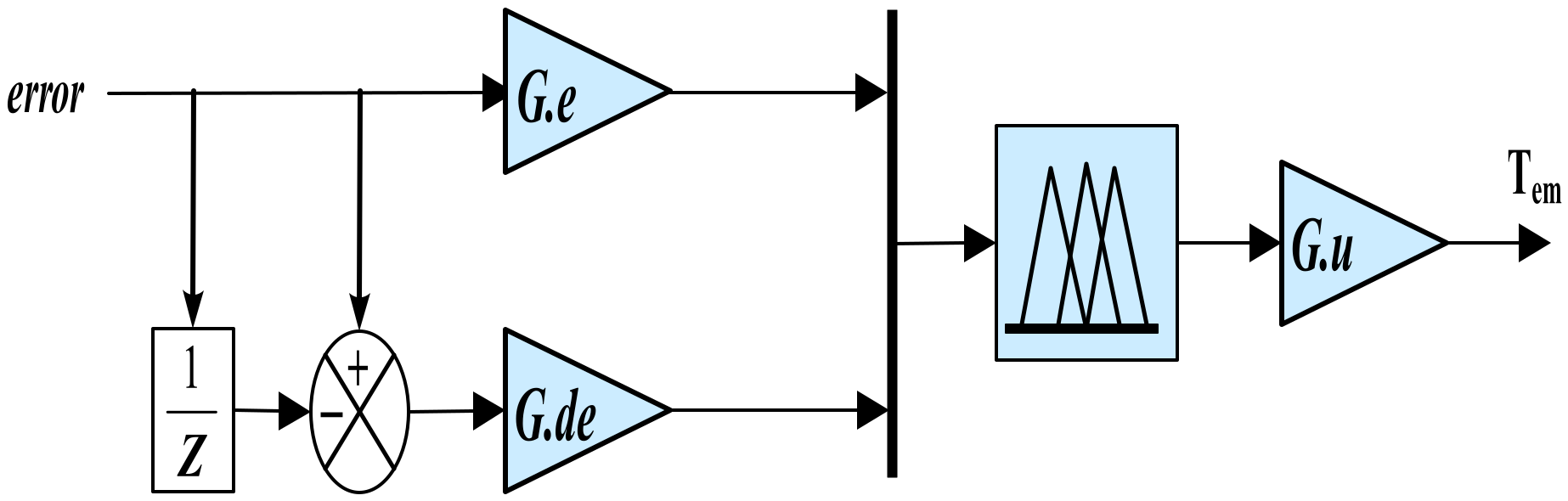
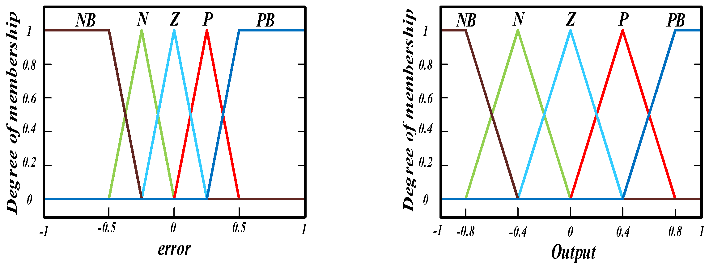
3.5. Fuzzy Logic Controller (FLC)

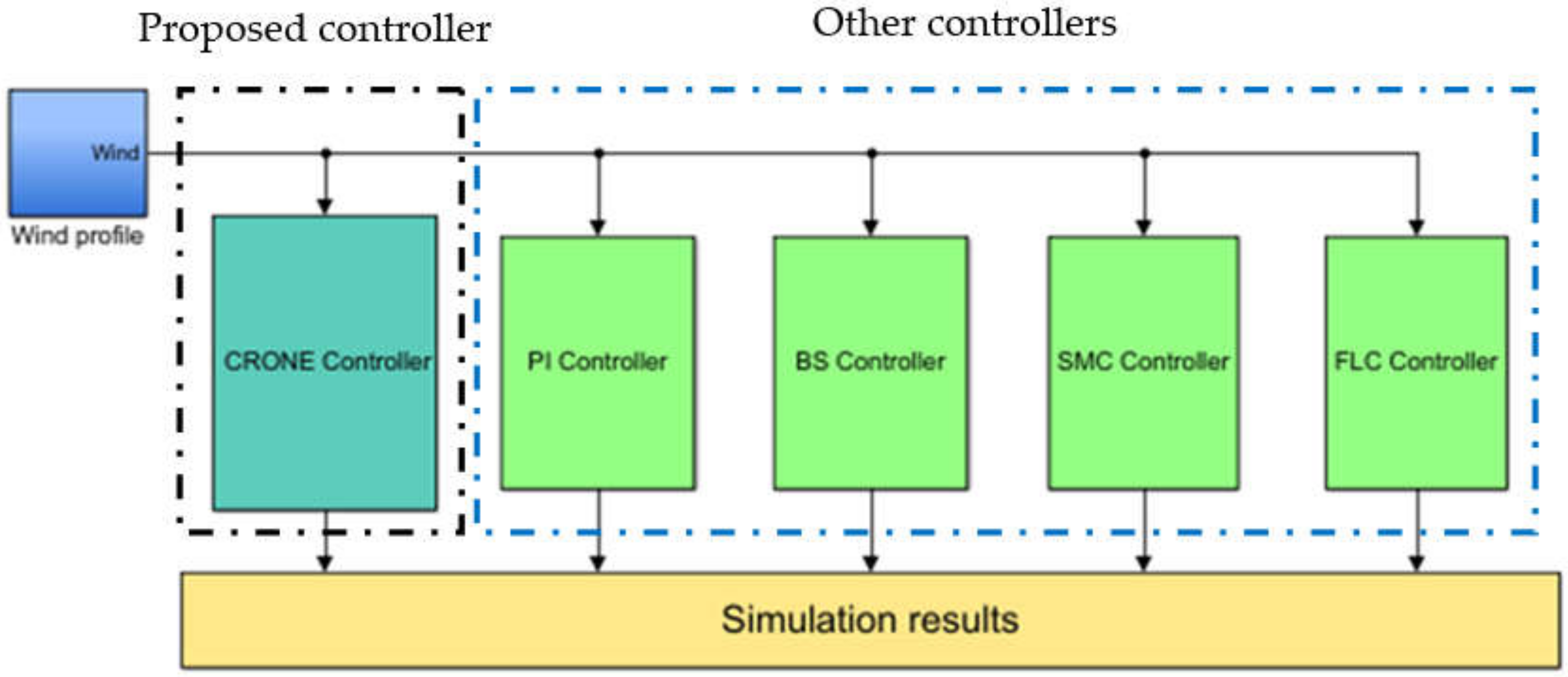
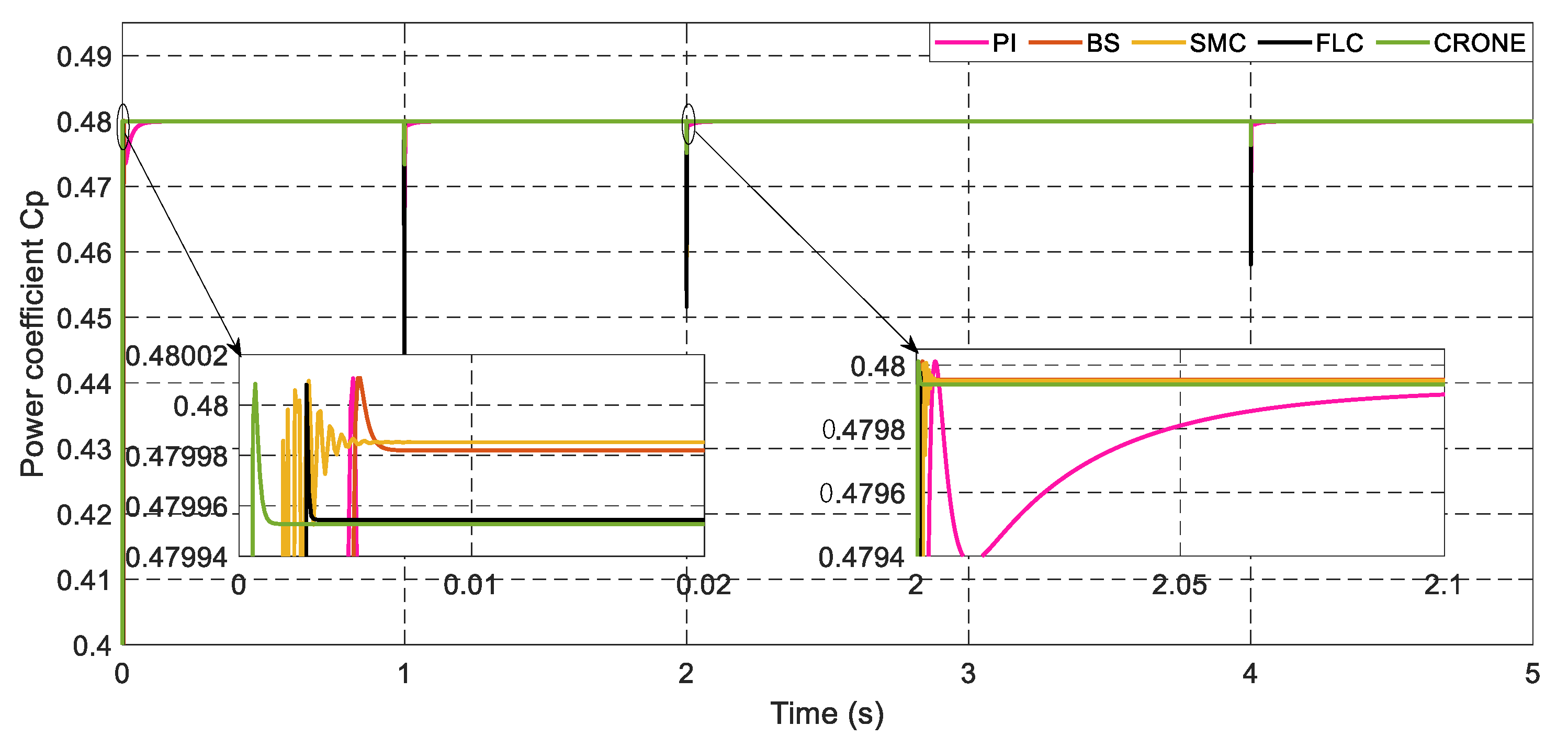
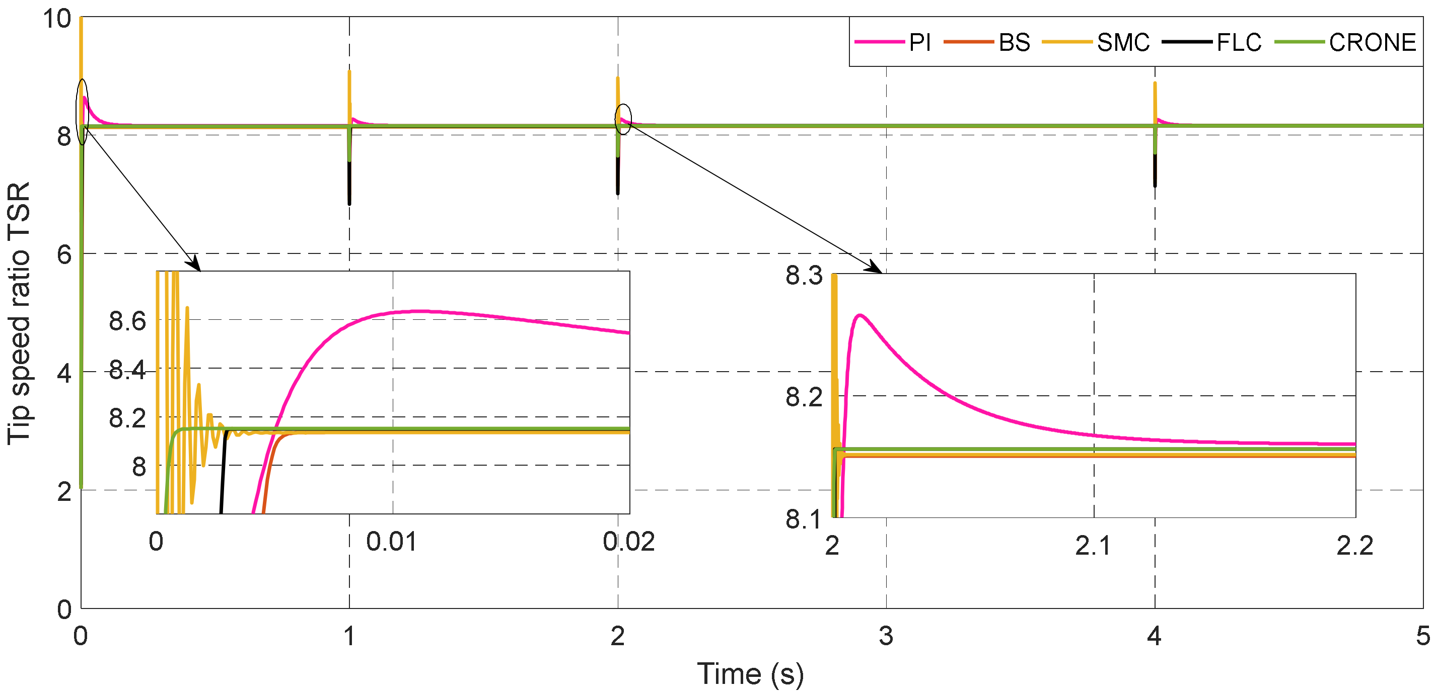
The design of a fuzzy controller is described in Figure 8. Such a controller is considered a robust and intelligent adaptive tool for complex non-linear systems. It requires the selection of the linguistic variables, the membership functions, the defuzzification strategy, and the method of inference [51]. This controller is employed to adjust the mechanical velocity in order to pursue the reference value for maximizing the extracted power of the turbine based on the rules presented in

Table 1. Set of rules generated for FLC.

Output		de(t)
		NB	N	Z	P	PB
e(t)	NB	NB	NB	N	N	Z
	N	NB	N	N	Z	P
	Z	NB	N	Z	P	P
	P	N	Z	P	P	PB
	PB	Z	P	P	PB	PB

, where ‘e’ (error speed) and ‘de’ are used as inputs, while Tem (electromagnetic torque) designates the output [52]. Consequently, the variables, which are mentioned above, are represented by NB, N, Z, P, and PB, indicating negative big, negative, zero, positive, and positive big, respectively [51,52].

The input and output functions of the triangular membership are described in Figure 9. They have seven fuzzy subsets. Furthermore, the fuzzy inference is performed based on the Sugeno technique, and the defuzzification uses the gravity center to identify the output of this FL control strategy [53].

4. Results

In this part of the paper, the performance of the proposed CRONE strategy is investigated and compared to others based on the following reference values: tracking, robustness, the dynamic response, the static error, and the system stability. The overall energy conversion system, considering a 1.5 MW wind turbine, was simulated using Matlab/Simulink (see Figure 10), with the presented parameters in

Table 2. Parameters of the turbine.

Parameters	Value
Number of blades	3
Blade radius R	35.25 m
Gearbox gain G	90
Friction coefficient (Fv)	2.4·10−3 N.m.s/rad
Moment of inertia (J)	1000 kg.m2

.

To validate the static and dynamic performance of the studied wind system in this paper, two different wind speed scenarios were applied for the simulation results.

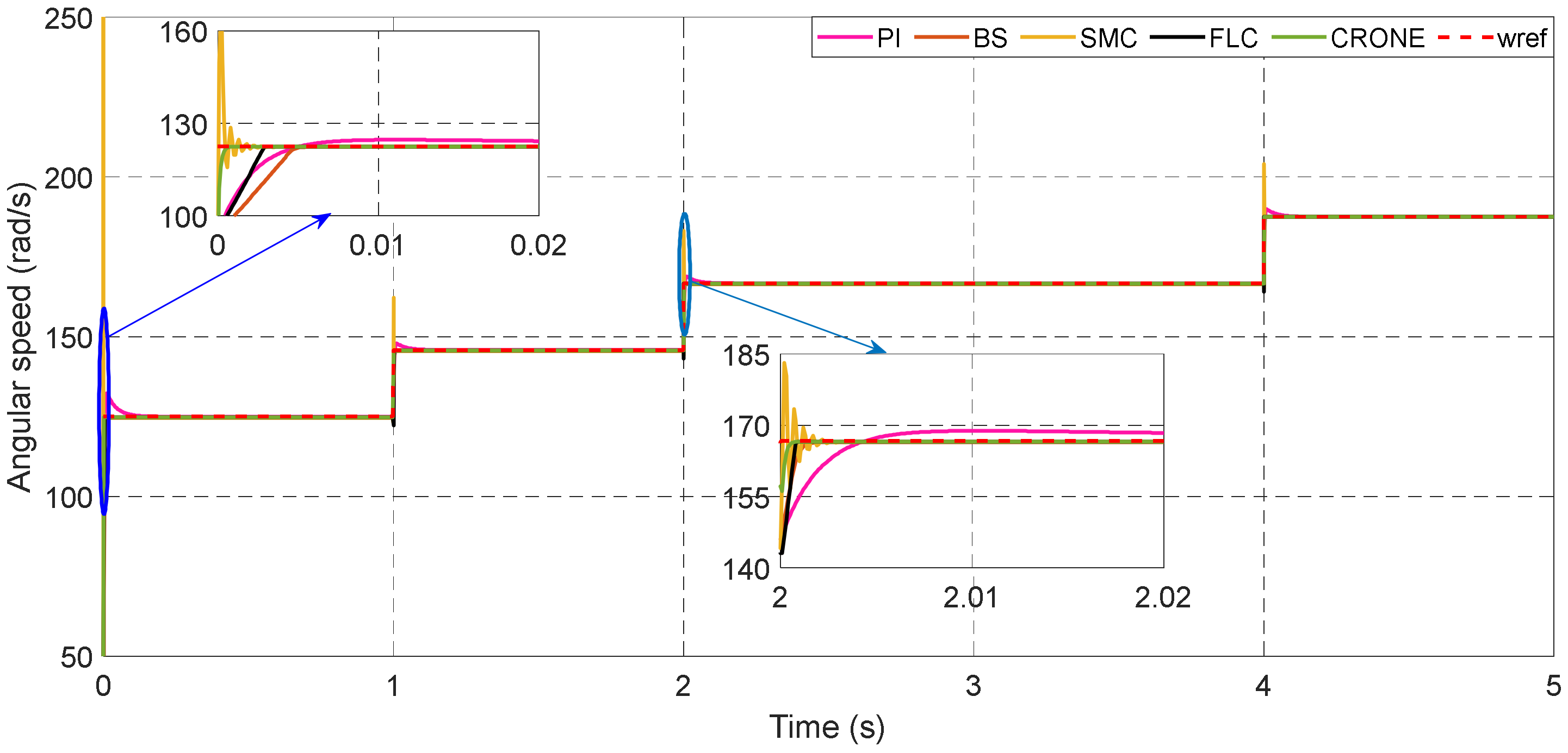
4.1. Tracking Test with Speed Step Profile

To determine the best choice of MPPT algorithm for a proposed variable wind speed turbine (VSWT), a tracking test must be performed for the control strategies to assess their merit in terms of being robust against radical changes in the wind profile, as shown in Figure 11. This wind profile is a standard profile used by the authors previously to compare various algorithms.

Figure 12, Figure 13, Figure 14 and Figure 15 show the static evolution of the five MPPT strategies with regard to mechanical velocity control. The obtained results clearly show that the dynamic performance of the system based on the CRONE controller is very efficient when compared to the other controllers, SMC, PI, BS, and FLC, under a moderate wind speed disturbance. With these variant conditions, it can be noted that the power coefficient C_p (Figure 12) takes a maximum value of 0.480015 for a blade pitch angle which is maintained at its minimum desired value (β = 0°).

The error close to the starting time (time zero) is high because the damping at the start of the turbine was very high at the beginning of the operation.

Based on these results and analysis, the second-generation CRONE controller was found to be the fastest in achieving the steady-state. Hence, the recovery time upon wind speed change was also faster for this algorithm. The PI controller, on the other hand, was found to be the slowest and least efficient method, as the response time was 166 times longer than the second-generation CRONE controller.

Table 3. Comparative study of the five MPPT controllers for a step wind profile.

Performance	PI	BS	SMC	FLC	CRONE
Response time (ms)	200	5.2	3.5	4	1.2
Static errors (%)	4.3	2.1	3.5	0.9	0.3
Set-point tracking	Good	Good	Good	Very good	Very good
Precision	Medium	Medium	High	Very high	Very high

, below, represents a qualitative and quantitative synthesis of the comparison of all five proposed controllers (PI, SMC, BS, FLC, and CRONE) in terms of the static error, response time, and set-point tracking precision.

The above simulation tests were necessary, but they are not sufficient to realistically validate the five controllers. Indeed, the test scenario does not represent a real wind profile in a real meteorological context. To deal with this problem, the studied methods were investigated with a real stochastic wind profile.

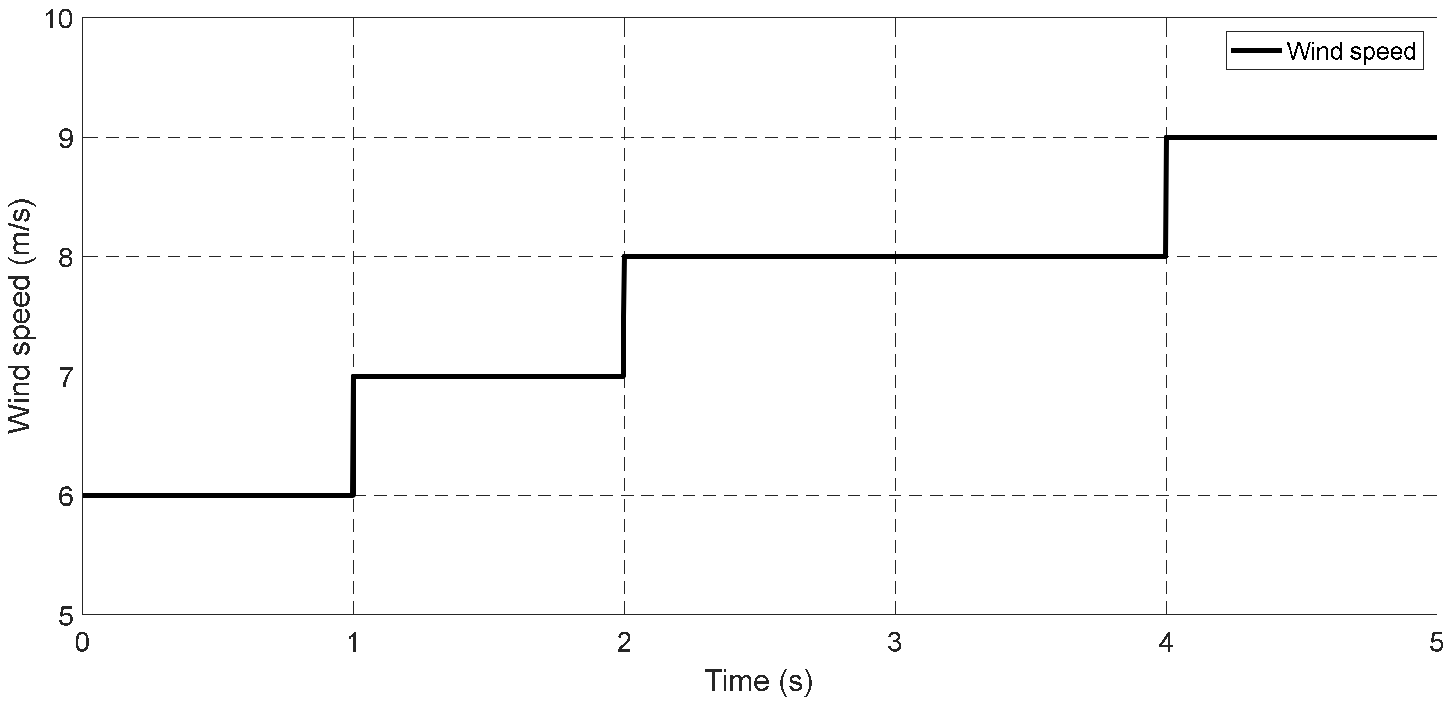
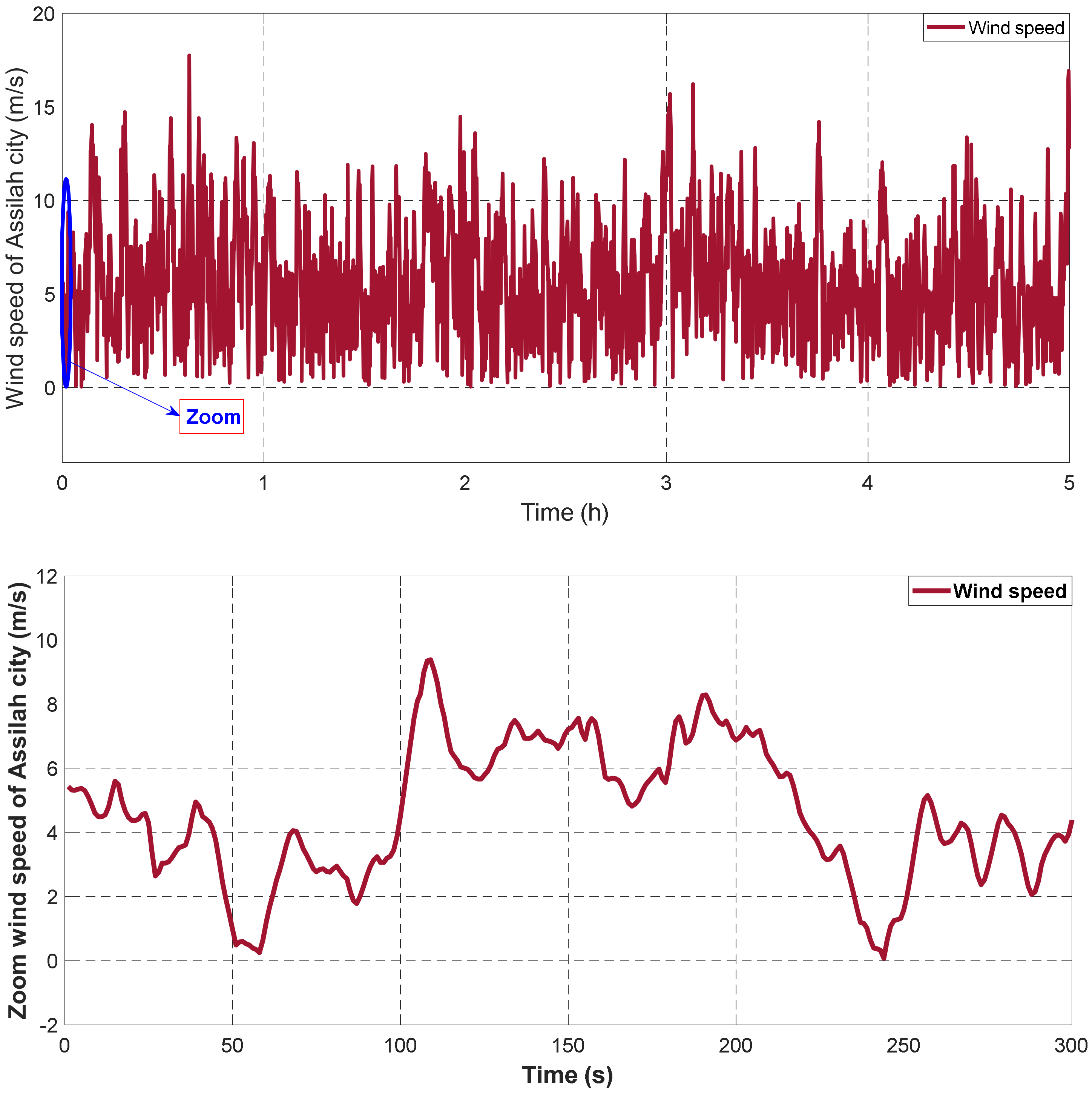
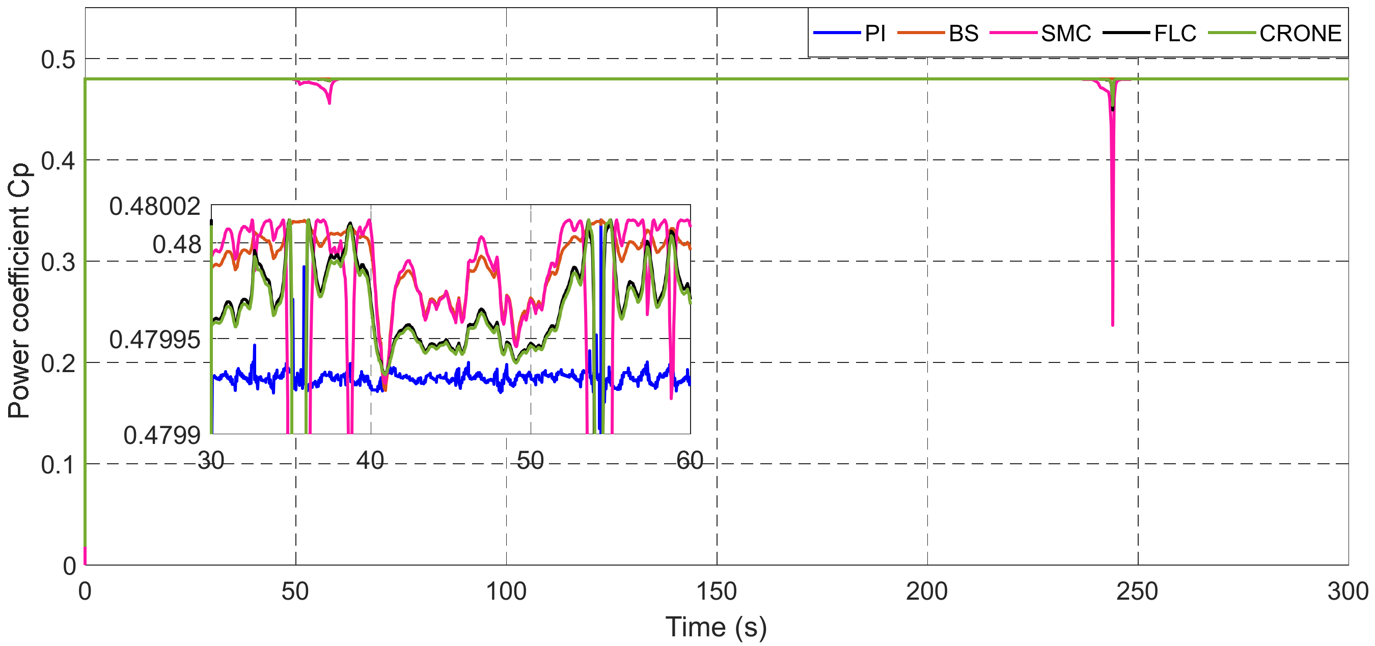
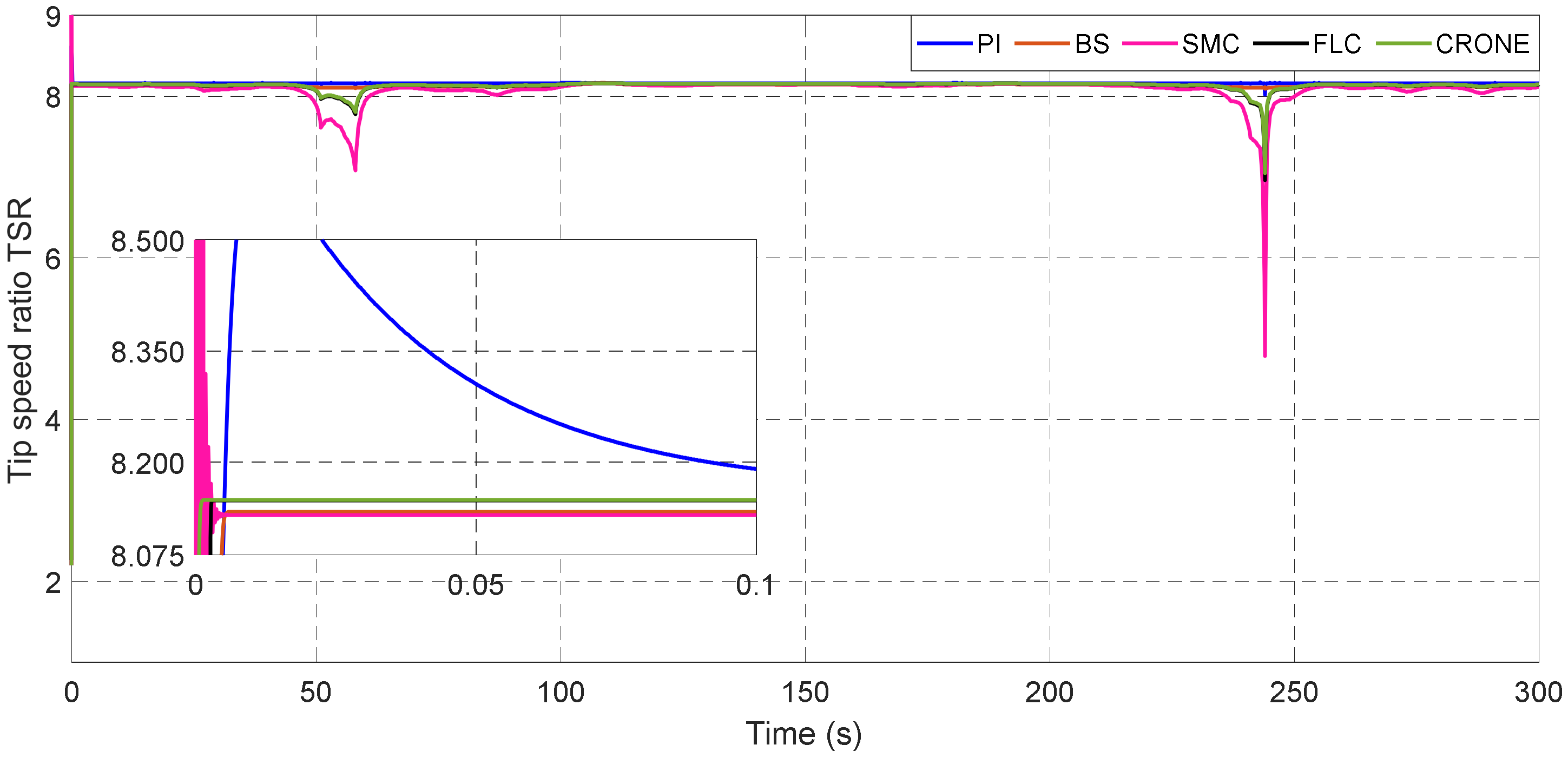
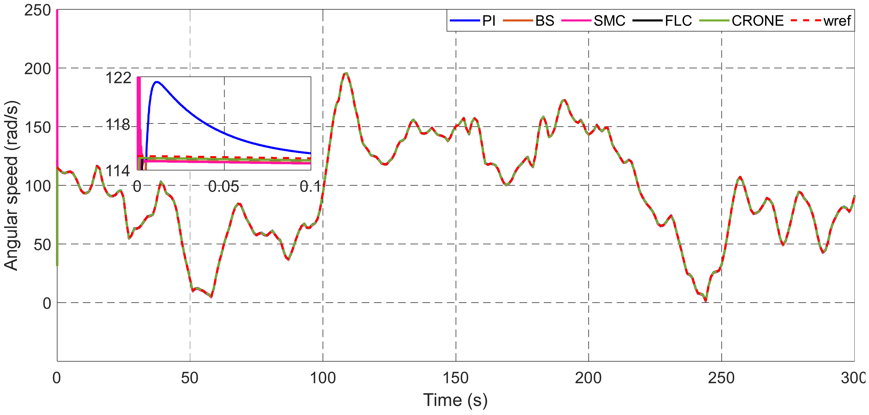
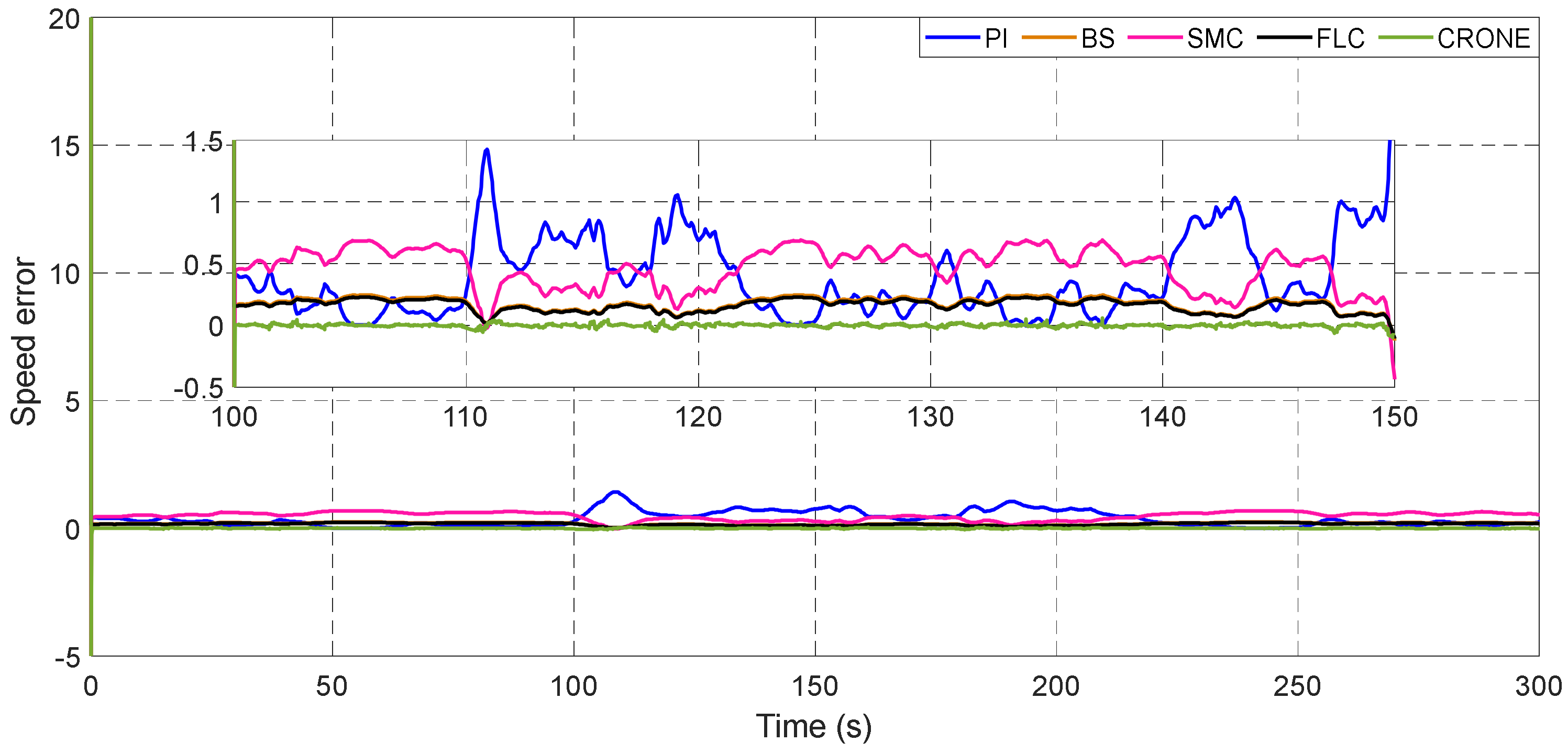
4.2. Tracking Test with Variable Real Wind Speed Profile

In this test, the simulated real wind profile of the city of Assilah in Morocco varies between 0 m/s and 13 m/s, as shown in Figure 16.

To extract the maximum value of supplied power, the speed ratio was fixed at the value λ_opt = 8.1 (Figure 13), which is in keeping with the maximum power coefficient C_pmax = 0.48 (Figure 16) for any wind speed variation.

The MPPT simulation results concerning the five proposed control methods (PI, SMC, BS, FLC, and CRONE) and a mechanical speed control law prove clearly that for each wind speed value, the mechanical speed perfectly followed its desired references in the case of all methods, but with disturbing significant static errors in the cases of the sliding mode and PI controllers, as can be seen in Figure 17, Figure 18, Figure 19 and Figure 20.

Moreover, it is noted that the CRONE controller and the fuzzy logic controller (FLC) methods both reached the static regime with small response times and a negligible static error. In contrast, the PI controller, the sliding mode controller (SMC), and the BS controller are characterized by a slightly slow response time, with minimal fluctuations in the case of the sliding mode controller (SMC) and a very important overshot in the cases of the PI and sliding mode controllers in the dynamics regime.

The error close to the starting time (time zero) is high because the damping at the start of the turbine was very high at the beginning of the operation.

Table 4. Comparative study for the real wind speed of Essaouira city, Morocco.

Performance	PI	BS	SMC	FLC	CRONE
Response time (ms)	255	6.4	5.5	4	2.1
Dynamic errors (%)	8.3	4.1	6.1	0.9	0.45
Set-point tracking	Good	Good	Good	Very good	Very good
Precision	Medium	Medium	High	Very high	Very high

below represents a qualitative and quantitative synthesis of the comparison of all five proposed controllers (PI, SMC, BS, FLC, and CRONE) in terms of the dynamic error, response time, and setpoint tracking precision. This table highlights the remarkable improvements obtained by the CRONE controller. In fact, among these improvements, the optimization of the response time, set-point tracking, precision, and dynamic error can be noted.

In order to position the proposed method in the field of research on MPPT strategies, a comparative study was realized between the proposed CRONE controller and two others control methods existing in two separate research papers. This study is illustrated in

Table 5. Comparative study between the proposed CRONE strategy and other works.

Reference Paper	MPPT Technique	Response Time (s)	Static Errors (%)	Set-Point Tracking
[16]	OTC	0.02488	--	Good
[54]	Backstepping	0.005	1.1	Good
Proposed method	CRONE	0.0012	0.3	Very good

. The comparison was carried out using several performance indexes.

It is clear that the CRONE controller provides the fastest response time compared to the other algorithms, and it represents a static error that is negligible.

5. Conclusions

This work was motivated by the efficiency and performance of the CRONE controller with respect to vehicles and HESG-based WECS systems. This motivation led the authors to test and implement this controller for a DFIG-based WECS for power wind turbine extraction.

In this study, the second-generation CRONE controller was designed and then tested against four MPPT strategies under a real wind profile. These controllers were a PI controller, a non-linear control based on sliding modes (SMC), a backstepping controller (BS), and a fuzzy logic controller (FLC).

The simulation results demonstrate that the application of the CRONE controller demonstrated the best performance and it proved to be the most suitable strategy for the chosen wind conversion power system in comparison with the other controllers studied in this work, whether in terms of the dynamic response, reference tracking, precision, static and dynamic error, or robustness. So, the second-generation CRONE controller will improve the performance of and overcome some of the obstacles found in current MPPT methods. This novel controller perfectly handles the problems of control effort level, and it significantly reduces the response time (0.0012 s).

Future work will address the validation of the best controller studied in this research paper using a real-time implementation in the dSPACE card.

References

1. Yessef, M.; Bossoufi, B.; Taoussi, M.; Lagrioui, A.; Chojaa, H. Improved Hybrid Control Strategy of the Doubly-Fed Induction Generator Under a Real Wind Profile. In Digital Technologies and Applications; ICDTA 2021. Lecture Notes in Networks and Systems; Motahhir, S., Bossoufi, B., Eds.; Springer: Cham, Switzerland, 2021; Volume 211. [Google Scholar] [CrossRef]
2. Hannachi, M.; Elbeji, O.; Benhamed, M.; Sbita, L. Optimal tuning of the proportional–integral controller using particle swarm optimization algorithm for control of permanent magnet synchronous generator based wind turbine with tip speed ratio for maximum power point tracking. Wind. Eng. 2021, 45, 400–412. [Google Scholar] [CrossRef]
3. Bekiroglu, E.; Yazar, M.D. MPPT Control of Grid Connected DFIG at Variable Wind Speed. Energies 2022, 15, 3146. [Google Scholar] [CrossRef]
4. Chhipa, A.A.; Kumar, V.; Joshi, R.R.; Chakrabarti, P.; Jasinski, M.; Burgio, A.; Leonowicz, Z.; Jasinska, E.; Soni, R.; Chakrabarti, T. Adaptive Neuro-Fuzzy Inference System-Based Maximum Power Tracking Controller for Variable Speed WECS. Energies 2021, 14, 6275. [Google Scholar] [CrossRef]
5. Pan, L.; Zhu, Z.; Xiong, Y.; Shao, J. Integral Sliding Mode Control for Maximum Power Point Tracking in DFIG Based Floating Offshore Wind Turbine and Power to Gas. Processes 2021, 9, 1016. [Google Scholar] [CrossRef]
6. Song, D.; Tu, Y.; Wang, L.; Jin, F.; Li, Z.; Huang, C.; Xia, E.; Rizk-Allah, R.M.; Yang, J.; Su, M.; et al. Coordinated optimization on energy capture and torque fluctuation of wind turbines via variable weight NMPC with fuzzy regulator. Appl. Energy 2022, 312, 118821. [Google Scholar] [CrossRef]
7. Chen, Z.; Yin, M.; Zou, Y.; Meng, K.; Dong, Z.Y. Maximum Wind Energy Extraction for Variable Speed Wind Turbines with Slow Dynamic Behavior. IEEE Trans. Power Syst. 2017, 32, 3321–3322. [Google Scholar] [CrossRef]
8. Rodríguez-Amenedo, J.L.; Arnaltes, S.; Rodríguez, M.A. Operation and Coordinated Control of Fixed and Variable Speed Wind Farms. Renew. Energy 2008, 33, 406–414. [Google Scholar]
9. Yessef, M.; Bossoufi, B.; Taoussi, M.; Lagrioui, A.; El Mahfoud, M. Evaluation of Adaptive Backstepping Control Applied to DFIG Wind System Used on the Real Wind Profile of the Dakhla-Morocco City. In WITS 2020. Lecture Notes in Electrical Engineering; Bennani, S., Lakhrissi, Y., Khaissidi, G., Mansouri, A., Khamlichi, Y., Eds.; Springer: Singapore, 2022; Volume 745. [Google Scholar] [CrossRef]
10. Bossoufi, B.; Karim, M.; Taoussi, M.; Aroussi, H.A.; Bouderbala, M.; Motahhir, S.; Camara, M.B. DSPACE-based implementation for observer backstepping power control of DFIG wind turbine. IET Electr. Power Appl. 2020, 14, 2395–2403. [Google Scholar] [CrossRef]
11. Taoussi, M.; Bossoufi, B.; Bouderbala, M.; Motahhir, S.; Alkhammash, E.H.; Masud, M.; Zinelaabidine, N.; Karim, M. Implementation and Validation of Hybrid Control for a DFIG Wind Turbine Using an FPGA Controller Board. Electronics 2021, 10, 3154. [Google Scholar] [CrossRef]
12. Zhou, F.; Liu, J. A Robust Control Strategy Research on PMSG-Based WECS Considering the Uncertainties. IEEE Access 2018, 6, 51951–51963. [Google Scholar] [CrossRef]
13. Abdullah, M.A.; Yatim, A.H.M.; Tan, C.W.; Saidur, R. A review of maximum power point tracking algorithms for wind energy systems. Renew. Sustain. Energy Rev. 2012, 16, 3220–3227. [Google Scholar] [CrossRef]
14. Kumar, D.; Chatterjee, K. A Review of Conventional and Advanced MPPT Algorithms for Wind Energy Systems. Renew. Sustain. Energy Rev. 2016, 55, 957–970. [Google Scholar] [CrossRef]
15. Elbeji, O.; Hannachi, M.; Benhamed, M.; Sbita, L. Maximum power point tracking control of wind energy conversion system driving a permanent magnet synchronous generator: Comparative study. Wind. Eng. 2021, 45, 1072–1081. [Google Scholar] [CrossRef]
16. Nasiri, M.; Milimonfared, J.; Fathi, S.H. Modeling, analysis and comparison of TSR and OTC methods for MPPT and power smoothing in permanent magnet synchronous generator-based wind turbines. Energy Convers. Manag. 2014, 86, 892–900. [Google Scholar] [CrossRef]
17. Hannachi, M.; Elbeji, O.; Benhamed, M.; Sbita, L. Comparative study of four MPPT for a wind power system. Wind. Eng. 2021, 45, 1613–1622. [Google Scholar] [CrossRef]
18. Abdullah, M.A.; Yatim, A.H.M.; Tan, C.W. An Online Optimum-Relation-Based Maximum Power Point Tracking Algorithm for Wind Energy Conversion System. In Proceedings of the 2014 Australasian Universities Power Engineering Conference, AUPEC 2014—Proceedings, Perth, WA, Australia, 28 September–1 October 2014. [Google Scholar]
19. Lalouni, S.; Rekioua, D.; Idjdarene, K.; Tounzi, A. Maximum Power Point Tracking Based Hybrid Hill-Climb Search Method Applied to Wind Energy Conversion System. Electr. Power Compon. Syst. 2015, 43, 1028–1038. [Google Scholar] [CrossRef]
20. Hosseini, S.H.; Farakhor, A.; Haghighian, S.K. Novel Algorithm of Maximum Power Point Tracking (MPPT) for Variable SpeedPMSG Wind Generation Systems through Model Predictive Control. In Proceedings of the ELECO 2013—8th International Conference on Electrical and Electronics Engineering, Bursa, Turkey, 28–30 November 2013; pp. 243–247. [Google Scholar]
21. Hohm, D.P.; Ropp, M.E. Comparative Study of Maximum Power Point Tracking Algorithms. Prog. Photovolt. Res. Appl. 2003, 11, 47–62. [Google Scholar] [CrossRef]
22. Cheng, M.; Zhu, Y. The State of the Art of Wind Energy Conversion Systems and Technologies: A Review. Energy Convers. Manag. 2014, 88, 332–347. [Google Scholar] [CrossRef]
23. Pagnini, L.C.; Burlando, M.; Repetto, M.P. Experimental Power Curve of Small-Size Wind Turbines in Turbulent Urban Environment. Appl. Energy 2015, 154, 112–121. [Google Scholar] [CrossRef]
24. Apata, O.; Oyedokun, D.T.O. An Overview of Control Techniques for Wind Turbine Systems. Sci. Afr. 2020, 10, e00566. [Google Scholar] [CrossRef]
25. Ata, R. Artificial Neural Networks Applications in Wind Energy Systems: A Review. Renew. Sustain. Energy Rev. 2015, 49, 534–562. [Google Scholar] [CrossRef]
26. Thongam, J.S.; Bouchard, P.; Ezzaidi, H.; Ouhrouche, M. Artificial Neural Network-Based Maximum Power Point Tracking Control for Variable Speed Wind Energy Conversion Systems. In Proceedings of the IEEE International Conference on Control Applications, St. Petersburg, Russia, 8–10 July 2009; pp. 1667–1671. [Google Scholar]
27. Song, D.; Li, Z.; Wang, L.; Jin, F.; Huang, C.; Xia, E.; Rizk-Allah, R.M.; Yang, J.; Su, M.; Joo, Y.H. Energy capture efficiency enhancement of wind turbines via stochastic model predictive yaw control based on intelligent scenarios generation. Appl. Energy 2022, 312, 118773. [Google Scholar] [CrossRef]
28. Moradi, H.; Vossoughi, G. Robust control of the variable-speed wind turbines in the presence of uncertainties: Acomparison between H∞ and PID controllers. Energy 2015, 90, 1508–1521. [Google Scholar] [CrossRef]
29. Mseddi, A.; Le Ballois, S.; Aloui, H.; Vido, L. Robust control of a wind conversion system based on a hybrid excitation synchronous generator: A comparison between H∞ and CRONE controllers. Math. Comput. Simul. 2019, 158, 453–476. [Google Scholar] [CrossRef]
30. Benine-Neto, X.; Moreau, P. Lanusse, Robust control for an electro-mechanical anti-lock braking system: The CRONE approach. IFAC-PapersOnLine 2017, 50, 12575–12581. [Google Scholar] [CrossRef]
31. Bouvin, J.L.; Moreau, X.; Benine-Neto, A.; Oustaloup, A.; Serrier, P.; Hernette, V. CRONE control of a pneumatic self-leveling suspension system. IFAC-PapersOnLine 2017, 50, 13816–13821. [Google Scholar] [CrossRef]
32. Hannachi, M.; Elbeji, O.; Benhamed, M.; Sbita, L. Optimal torque maximum power point technique for wind turbine: Proportional–integral controller tuning based on particle swarm optimization. Wind. Eng. 2021, 45, 337–350. [Google Scholar] [CrossRef]
33. Lanusse, P.; Sabatier, J.; Nelson Gruel, D.; Oustaloup, A. Second and Third Generation CRONE Control-System Design. In Fractional Order Differentiation and Robust Control Design. Intelligent Systems, Control and Automation: Science and Engineering; Springer: Dordrecht, The Netherlands, 2015; Volume 77. [Google Scholar] [CrossRef]
34. Oustaloup, A. Systèmes Asservis Linéaires D’ordre Fractionnaire; Masson: Paris, France, 1983. [Google Scholar]
35. Oustaloup, A. La Commande CRONE; Hermes Editor: Paris, France, 1991. [Google Scholar]
36. Oustaloup, A.; Mathieu, B.; Lanusse, P. The CRONE control of resonant plants: Application to a flexible transmission. Eur. J. Control. 1995, 1, 113–121. [Google Scholar] [CrossRef]
37. Lanusse, P. De la Commande CRONE de Première Génération à la Commande CRONE de Troisième Generation. Ph.D. Thesis, University Bordeaux I, Bordeaux, France, 1994. [Google Scholar]
38. Åström, K.J. Model Uncertainty and Robust Control Design; COSY Workshop, ESF Course: Valencia, Spain, 1999. [Google Scholar]
39. Lanusse, P.; Oustaloup, A.; Sabatier, J. Step-by-step presentation of a 3rd generation CRONE controller design with an anti-windup system. In Proceedings of the Fifth EUROMECH Nonlinear Dynamics Conference, Eindhoven, The Netherlands, 7–12 August 2005. [Google Scholar]
40. Lanusse, P.; Oustaloup, A.; Sutter, D. Multi-scalar CRONE control of multivariable plants. In Proceedings of the WAC’96-ISIAC Symphosia, Montpellier, France, 27–30 May 1996. [Google Scholar]
41. Lanusse, P.; Malti, R.; Melchior, P. CRONE control system design toolbox for the control engineering community: Tutorial and case study. Philos. Trans. R. Soc. A 2012, 371, 0149. [Google Scholar] [CrossRef] [Green Version]
42. Bode, H.W. Network Analysis and Feedback Amplifier Design; Van Nostrand: New York, NY, USA, 1945. [Google Scholar]
43. CRONE Toolbox. Available online: http://cronetoolbox.ims-bordeaux.fr (accessed on 21 April 2022.).
44. Xiao, F.; Zhang, Z.; Yin, X. Fault Current Characteristics of the DFIG under Asymmetrical Fault Conditions. Energies 2015, 8, 10971–10992. [Google Scholar] [CrossRef] [Green Version]
45. Bossoufi, B.; Karim, M.; Taoussi, M.; Aroussi, H.A.; Bouderbala, M.; Deblecker, O.; Motahhir, S.; Nayyar, A.; Alzain, M.A. Rooted Tree Optimization for the Backstepping Power Control of a Doubly Fed Induction Generator Wind Turbine: dSPACE Implementation. IEEE Access 2021, 9, 26512–26522. [Google Scholar] [CrossRef]
46. Taoussi, M.; Karim, M.; Bossoufi, B.; Hammoumi, D.; El Bakkali, C.; Derouich, A.; El Ouanjli, N. Low-Speed Sensorless Control for Wind Turbine System. WSEAS Trans. Syst. Control. 2017, 12, 405–417. [Google Scholar]
47. Yessef, M.; Bossoufi, B.; Taoussi, M.; Lagrioui, A. Enhancement of the direct power control by using backstepping approach for a doubly fed induction generator. Wind. Eng. 2022. [Google Scholar] [CrossRef]
48. Yessef, M.; Bossoufi, B.; Taoussi, M.; Lagrioui, A.; Chojaa, H.; Majout, B.; El Alami, H. Robust Control of a Wind Conversion System Based on a Doubly Fed Induction Generator: A Comparison Between Adaptive Backstepping and Integral Sliding Mode Controllers. In Digital Technologies and Applications; ICDTA 2022. Lecture Notes in Networks and Systems; Motahhir, S., Bossoufi, B., Eds.; Springer: Cham, Switzerland, 2022; Volume 454. [Google Scholar] [CrossRef]
49. Chojaa, H.; Derouich, A.; Chehaidia, S.E.; Zamzoum, O.; Taoussi, M.; Elouatouat, H. Integral sliding mode control for DFIG based WECS with MPPT based on artificial neural network under a real wind profile. Energy Rep. 2021, 7, 4809–4824. [Google Scholar] [CrossRef]
50. Li, P.; Xiong, L.; Wu, F.; Ma, M.; Wang, J. Sliding mode controller based on feedback linearization for damping of sub-synchronous control interaction in DFIG-based wind power plants. Int. J. Electr. Power Energy Syst. 2019, 107, 239–250. [Google Scholar] [CrossRef]
51. Chojaa, H.; Derouich, A.; Taoussi, M.; Zamzoum, O.; Yessef, M. Optimization of DFIG Wind Turbine Power Quality Through Adaptive Fuzzy Control. In Digital Technologies and Applications; ICDTA 2021. Lecture Notes in Networks and Systems; Motahhir, S., Bossoufi, B., Eds.; Springer: Cham, Switzerland, 2021; Volume 211. [Google Scholar] [CrossRef]
52. Aissaoui, H.E.; Ougli, A.E.; Tidhaf, B. Neural Networks and Fuzzy Logic Based Maximum Power Point Tracking Control for Wind Energy Conversion System. Adv. Sci. Technol. Eng. Syst. J. 2021, 6, 586–592. [Google Scholar] [CrossRef]
53. Tiwari, R.; Babu, N.R. Fuzzy logic based MPPT for permanent magnet synchronous generator in wind energy conversion system. IFAC 2016, 49, 462–467. [Google Scholar] [CrossRef]
54. Nadour, M.; Essadki, A.; Nasser, T. Comparative analysis between PI & backstepping control strategies of DFIG driven by wind turbine. Int. J. Renew. Energy Resour. 2017, 7, 1307–1316. [Google Scholar]
Figure 1. Different operation zones of a wind turbine.
Energies 15 03644 g001
Figure 2. Power coefficient as a function of λ and β.
Energies 15 03644 g002
Figure 3. Aerodynamic model of the wind turbine.
Energies 15 03644 g003
Figure 4. MPPT Strategy with speed control.
Energies 15 03644 g004
Figure 5. CRONE Control System Design diagram.
Energies 15 03644 g005
Figure 6. Bode plot of the controlled open-loop.
Energies 15 03644 g006
Figure 7. Typical regulator PI structure.
Energies 15 03644 g007
Figure 8. Fuzzy logic MPPT controller.
Energies 15 03644 g008
Figure 9. Inputs and output membership degree.
Energies 15 03644 g009
Figure 10. Matlab/Simulink architecture of the designed controllers.
Energies 15 03644 g010
Figure 11. Wind step speed profile (m/s).
Energies 15 03644 g011
Figure 12. Power coefficient for PI, BS, SMC, FLC, and CRONE controllers.
Energies 15 03644 g012
Figure 13. Tip speed ratio for PI, BS, SMC, FLC, and CRONE controllers.
Energies 15 03644 g013
Figure 14. Angular rotor speed for PI, BS, SMC, FLC, and CRONE controllers.
Energies 15 03644 g014
Figure 15. Speed error for PI, BS, SMC, FLC, and CRONE controllers.
Energies 15 03644 g015
Figure 16. Wind speed profile of Assilah, Morocco.
Energies 15 03644 g016
Figure 17. Power coefficient for PI, BS, SMC, FLC, and CRONE controllers.
Energies 15 03644 g017
Figure 18. Tip speed ratio for PI, BS, SMC, FLC, and CRONE controllers.
Energies 15 03644 g018
Figure 19. Angular rotor speed for PI, BS, SMC, FLC, and CRONE controllers.
Energies 15 03644 g019
Figure 20. Speed error for PI, BS, SMC, FLC, and CRONE controllers.
Energies 15 03644 g020