1. Introduction
The search for truly sustainable sources of energy has translated into renewed interest in low-power, low-impact small-scale hydraulic power devices. Those devices notably include devices that bypass traditional dam-based installations, whose biological and hydropower performance were investigated in recent research [
1,
2], as well as hydrokinetic turbines (e.g., [
3,
4]), which may be installed on floating or unchanneled installations. One type of hydrokinetic device that is of particular interest in this work is the free-stream water wheel.
Free-stream water wheels last made significant contributions to power production in 19th Century Europe [
5]. They consist of a partially immersed rotor with a horizontal rotation axis mounted perpendicular to the flow. The device rests floating at the surface of the river, exposed to undisturbed water flow without any kind of obstruction to the river’s biological continuity. This type of device is often suggested for power generation due to its minimal effect on aquatic life. Modern studies of similar devices in the scientific literature include [
6,
7,
8,
9,
10], as well as [
11,
12,
13,
14,
15]—see our coverage of this literature in [
16,
17]; a good review is provided in [
18].
Research inspired by the
Fluss-Strom consortium with support from the German Federal Ministry of Education and Research [
19] has allowed for the investigation of the hydraulic power performance of free-stream water wheels. First, the physical limits constraining the performance of such machines were described in [
20]. In a second step, the key performance characteristics of the free-stream wheel were identified in [
16]. To this purpose, a family of 30 two-dimensional computational fluid dynamics (
cfd) simulations had been set up, backed by experimental validation on a small-scale model. The study, in which various geometrical and operational parameters were varied, allowed observing and quantifying phenomena such as negative power delivery during the entry of the blades into the water (“splash-in” losses), as well as at the exit due to water pickup (“splash-out” losses). The main performance metrics of interest had been identified as the hydraulic power coefficient (the ratio of power produced at the shaft to the hydraulic power corresponding to the immersed blade frontal area, later defined in Equation (
6)), and the rotor power coefficient (the ratio of power produced at the shaft to the hydraulic power corresponding to the total wheel frontal area, defined in Equation (
7) further down).
In subsequent research, an optimisation study was carried out [
17], attempting to maximise both the hydraulic and rotor power coefficients of such wheels using two-dimensional
cfd simulations. In that study, the blade geometry was parametrised as a single relaxed spline connecting three points, whose position was determined using two angles. In total, five parameters were varied, resulting in a very large breadth of possible designs of various depths and radii. The
cfd simulations were steered by a genetic optimisation algorithm. After nearly 2000 evaluations had been carried out, a set of design guidelines was proposed, describing a Pareto-optimal family of wheels. General trends were also described, concluding that the operators seeking to maximise power, without a constraint on the production cost of the wheel or the depth of the river, should opt for larger wheels with lower depth relative to the radius of the wheel, while those operators with a lower budget should choose smaller wheels with a higher depth relative to the radius of the wheel.
Energy losses associated with blade splash-in and splash-out were a point of interest in this previously published study. In particular, it was observed that when the geometry was such that the blades would be fully immersed at the nadir point, those losses would be reduced. A preliminary study distinct from the optimisation was then conducted, indicating that increasing the radius of the blades’ root resulted in significantly smoother power delivery.
The objective of the present work is to further explore this design trend. In addition to reducing splash-in and -out losses, increasing the blades’ root radius (thus making them shorter) results in lower material usage and lighter structural requirements. Nevertheless, a trade-off is to be expected, since power delivery will obviously tend towards zero as the blades’ area tends to zero. Importantly, this trade-off may depend on the wheel configuration, and conversely, the optimum design parameters identified in [
17] may need to be re-evaluated when the blades are shortened.
In the present work, a dual-objective optimisation is conducted using a genetic algorithm, on the basis of two-dimensional cfd simulations. The optimisation considers a range of geometrical designs for a given wheel diameter, attempting to simultaneously maximise both the smoothness of the power delivery and the power output. In this manner, the present paper sets to answer the question: “Which optimal blade geometry or geometries result in the most valuable output for the operator of the free-stream water wheel?”. It will be shown that the optimisation results point towards a single design with fully immersed blades, resulting in a more reactive and more powerful design than those identified in previous research.
2. Blade Geometry and Performance Characterisation
The free-stream water wheel geometry considered in this work is shown in
Figure 1. The geometry of a single blade, a relaxed spline connecting three points positioned using two angles (
and
), is based on the design presented in the previously published optimisation [
17]. The tip radius (
R) is a set constant, at
(corresponding to one of the top-performing wheels in the previous study). Notably, the altitude of the blade root (measured with
, the vertical distance from the horizon line to the root of the blade, positive downwards) is now a variable. A new nondimensional parameter,
, is thus introduced as below:
The performance analysis tool used in this work was introduced in [
16]. It is recalled briefly again here, since it is useful in describing the performance and power delivery mechanism for the free-stream water wheel. In later sections, this tool will be used to compare different design configurations and evaluate their performance.
The depth
of the wheel is nondimensionalised as the wet radius fraction
by dividing by the tip radius
R, as shown below:
As shown in
Figure 1,
is the angle between the blade tip water entry and exit. The position of the blade during the power stroke is measured as the stroke angle
(varying along the path of the blade in water). It is nondimensionalised as
.
The number of blades
is also parametrised as an equivalent number of blades
, which represents the mean number of blades below the horizon line:
The hydraulic power output of the wheel is nondimensionalised as
as below:
As detailed in [
16], when the performance of the wheel is to be measured relative to its hydraulic footprint, the hydraulic power coefficient
is used:
where
is the rotor width. Conversely, when the performance of the wheel is to be measured relative to its own, full size, the rotor power coefficient
is used:
The power developed by any water wheel is deconstructed in terms of the contributions of individual blades by averaging out the blade power coefficient
over a number of blades (
), which can be later used to recover an averaged hydraulic power. In this way, as detailed in [
16], a single plot of
and
is able to describe the power output of the complete wheel, as used later in
Section 5.4.
Finally, an important performance indicator for free-stream wheels is the smoothness of the mechanical power delivery. Previous work has shown that blade splash-in, in particular, results in short-duration, high-intensity power absorption by the blades when they enter the water. In this way, power is temporarily lost by the rotor in favour of the water. This highly undesirable phenomena is quantified using the work ratio
(in which ntg stands for “net-to-gross”), defined according to Equation (
8) below.
Low values of work ratio are indicative that significant power is expended by the rotor in favour of the water during the travel of the blades. When , on the contrary, no energy is ever lost by the blades.
3. Optimisation Setup
3.1. Objective Functions
In contrast to the study it builds upon [
17], the present optimisation study focuses on reducing internal energy losses associated with blade entry and exit from the water. The study considers a wheel with a given radius and depth; thus, the hydraulic and rotor power coefficients vary monotonically together and do not need to be considered both at once. By contrast, the quality of the power delivery is of great interest here. Therefore, the two objectives pursued simultaneously in this work are:
3.2. Numerical Model
The reference simulation model used for the present optimisation study was carried over from [
16,
17], in which it was described in detail. For brevity, only a brief summary of numerical settings is given, summarised in
Table 1.
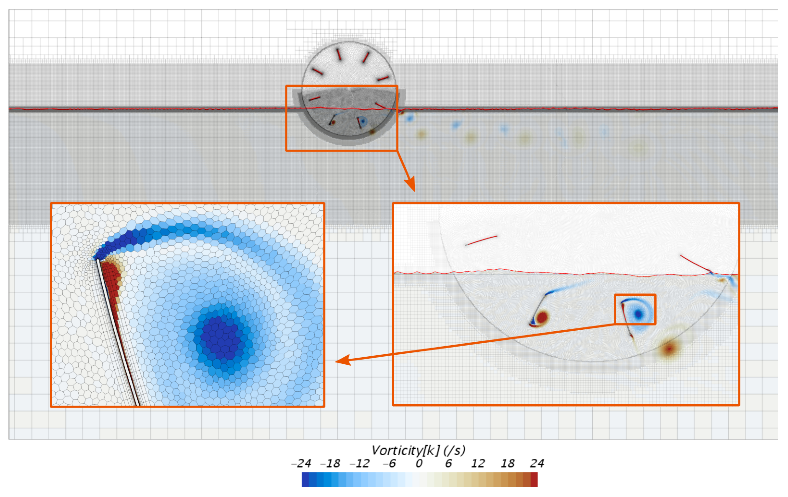
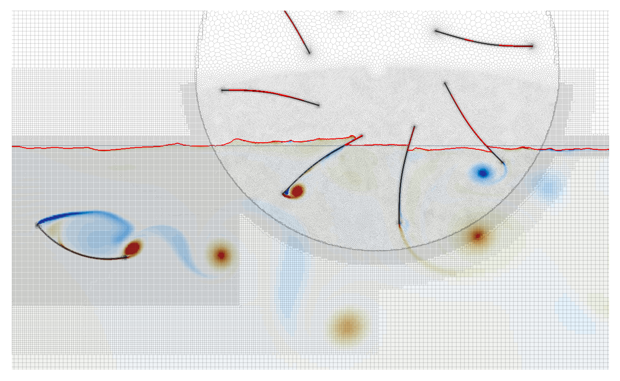
The meshes are periodically re-meshed to provide local refinement near the water surface. One simulation case, with generated vortices after 15
of physical time, is shown in
Figure 2 as a reference visualisation. The mesh refinement zones and flow domain are also represented there.
The computational domain has a width of 35
and height of 19
. The position of the centre of the wheel is constant across simulations and located at 15
from the inlet and 13
from the bottom of the domain. This simulation model has been already validated by experimental work in [
16], with power values reproduced with less than a 10% difference and identical trends. It was also shown that the results obtained in the reference simulation model were independent of the grid size. In the present study, additional surface refinement was carried out at the root of the blades, but all other settings were left intact.
The simulations were run with a time step of 10−3 s until 15 s of time elapsed. The power transmitted by each blade at every time step (except for the initial 3 s, during which the flow settles) was extracted as csv files and post-processed using in-house Python scripts.
3.3. Design Variables
In principle, the main input variable of interest—the fraction
, which determines to what extent the blades are shortened—may simply have been added to the input parameters considered in the previous study. Those are the wheel tip radius tip
R, the wet radius fraction
, the number of blades (
), and the two pivot angles (
,
), which determine the blade geometry. Doing so would have brought the total number of possible design configurations to 4.6 million. The number of variables and their range were thus limited, with consideration of the high computational and human costs involved. Thus, two input parameters, the wet radius fraction (
) and the tip radius (
R), were kept constant with a fixed value of 0.5 and
, respectively, which further means that the immersed depth of the wheel was fixed at
according to Equation (
2); this already reduced the number of the possible design configurations to 56,784. Furthermore, the ranges of the parameters were narrowed down based on knowledge obtained during the previous optimisation carried out in [
17], avoiding well-identified combinations that resulted in very low, sometimes purely negative, power output. This reduced the scope to a great extent, with 3600 possible design configurations after applying all constraints. To produce reliable results, it was expected that an optimum would be reached after evaluating approximately 10% of the domain, making the study feasible given the computational budget available.
For the current optimisation study, values of
were taken in intervals of 0.1 from −0.2 (with the root of the blade protruding above the horizon, as with most conventional designs) to 0.9 (for which the blade occupies only 0% of the wet frontal area), for a total of 12 discrete values. This range and those of the other input parameters are summarised in
Table 2. The free-stream inlet velocity (
) and tip-speed ratio were set to
/
and 0.5 throughout the optimisation study.
3.4. Software and Hardware Setup
The software selected to carry out the optimisation proper is the
moga genetic optimisation module of Dakota 6.10 [
21], a widely used open-source toolbox.
Individual instances of the parametrised cfd simulations were spawned by Dakota, running on a low-power desktop computer. Those simulation setups were then transferred using bash shell scripts to the “Neumann” high-performance cluster of the University of Magdeburg; each simulation (scripted using Java macros) was then run using Star-ccm+ on a single 16-cpu node after going through the job queue system. Once the simulation was complete, essential output data would be queried back to the desktop computer, where Python scripts would post-process the results and pass them back to Dakota.
4. Optimisation Process
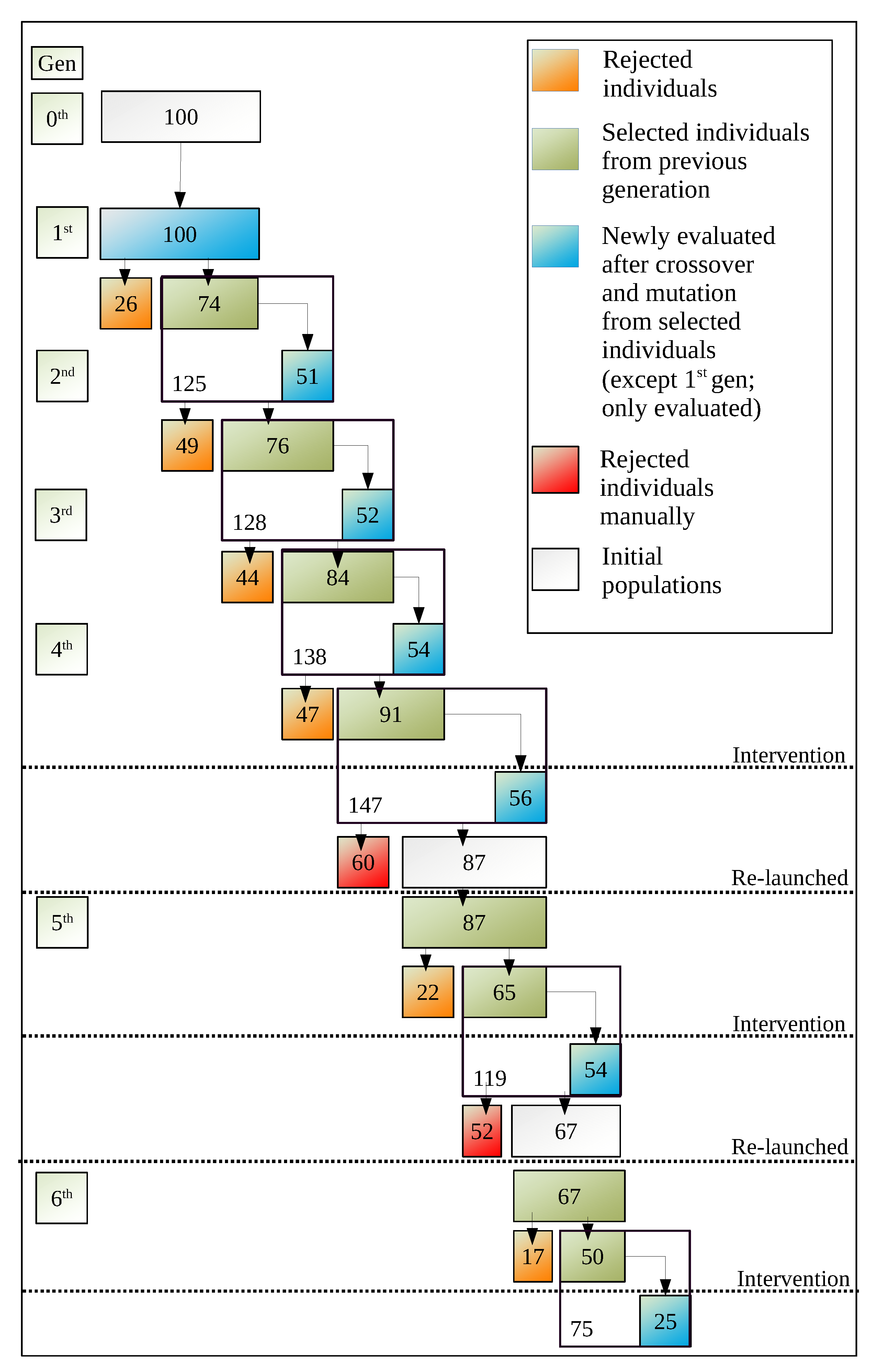
The optimisation loop was initialised with a first generation of 100 candidates, 12 of which were based on geometries known to perform well in the previous study, while the other 88 were constructed using Dakota’s Latin hypersquare algorithm (lhs). Initially, as a part of the first phase, the fitness of these 100 evaluated candidates was appraised by Dakota, and it carried out a selection based on their fitness. Only individuals in the five ranks closest to the latest Pareto front were selected; the remaining were rejected. These selected individuals were used as the input for the crossover and mutation operations, in order to constitute the next generation.
Crossover was performed between randomly selected parents, and mutation was also performed between candidates from the pool of selected individuals, in order to generate new individuals in each generation. These newly created individuals, characterised by a new set of input parameters, were then sent for evaluation by Star-
ccm+ in order to evaluate the value of objective functions in the next generation. The resulting evaluated candidates were then sent back to Dakota for selection, and the process moved forward until either convergence was reached or the optimisation was interrupted. The flow of individual evaluations during the optimisation in this paper is presented in
Figure 3.
In order for the genetic optimisation to converge meaningfully, the instantaneous Pareto front must be uniformly populated. Over the first four generations of the optimisation, it was observed that large regions within the Pareto front had no individuals. Therefore, the optimisation was interrupted, and more aggressive crossover and mutation settings were applied. Those settings are listed in
Table 3; they were used to re-launch the optimisation study, effectively starting the fifth generation based on a manual selection of the top 30% of the designs in the fourth generation. Two similar manual interventions were performed in the following generations, in order to ensure that the optimisation was converging appropriately.
When the present study completed, a total of 392 unique designs were explored. The evaluation of these designs took a total of 66,000 cpu-hours over three months.
5. Results and Analysis
5.1. Best-Performing Individuals
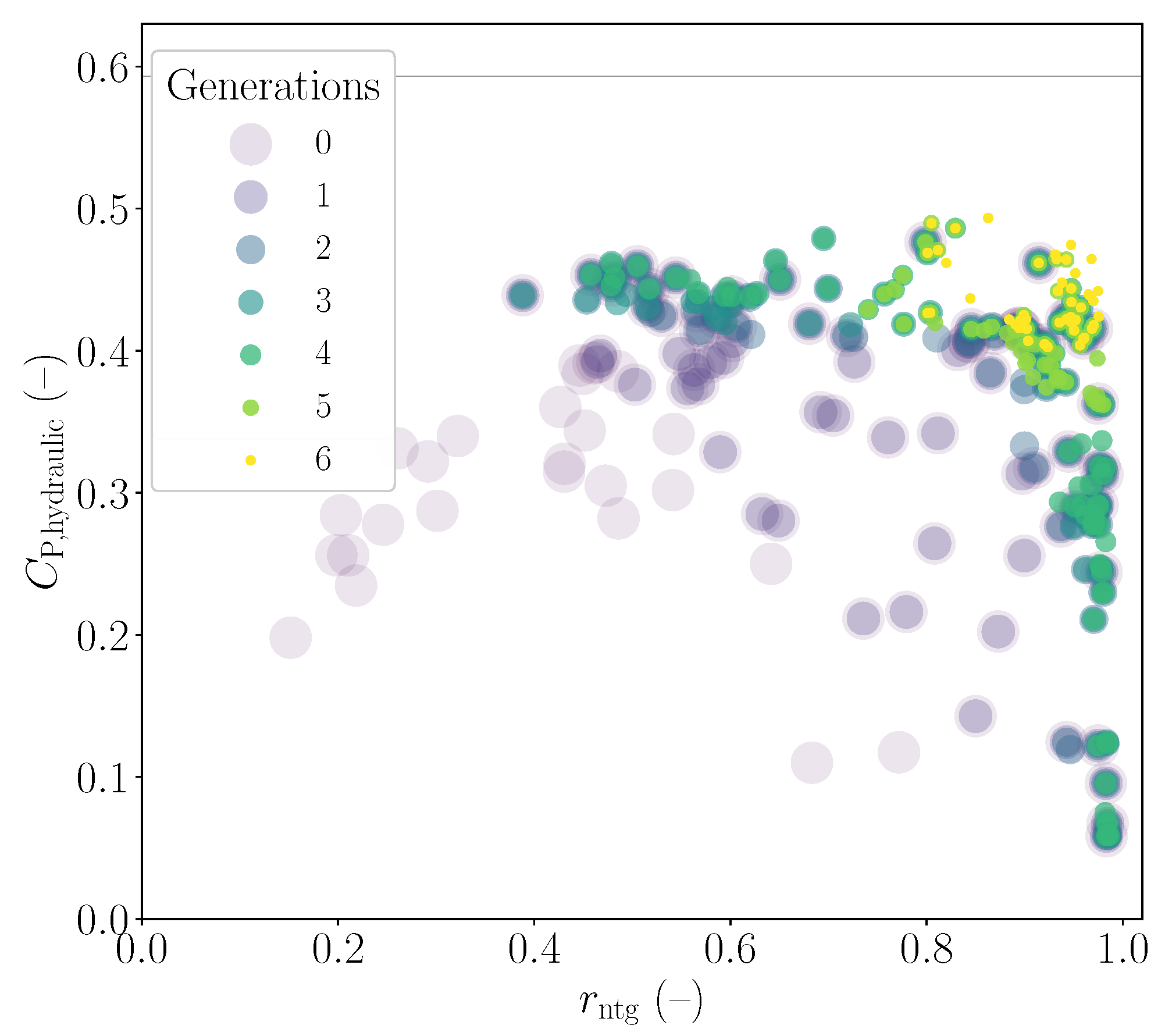
The performance of all candidates in every generation is plotted in
Figure 4, where the horizontal and vertical axes respectively represent
and
, the two objective functions to be maximised. There, candidates of later generations are depicted with smaller, lighter-coloured dots. It can be observed from the figure that after the fourth generation, two groups of candidates, each favouring one objective, emerged. As the optimisation reached the sixth generation, the performance of the selected individuals converged towards the top right of the figure.
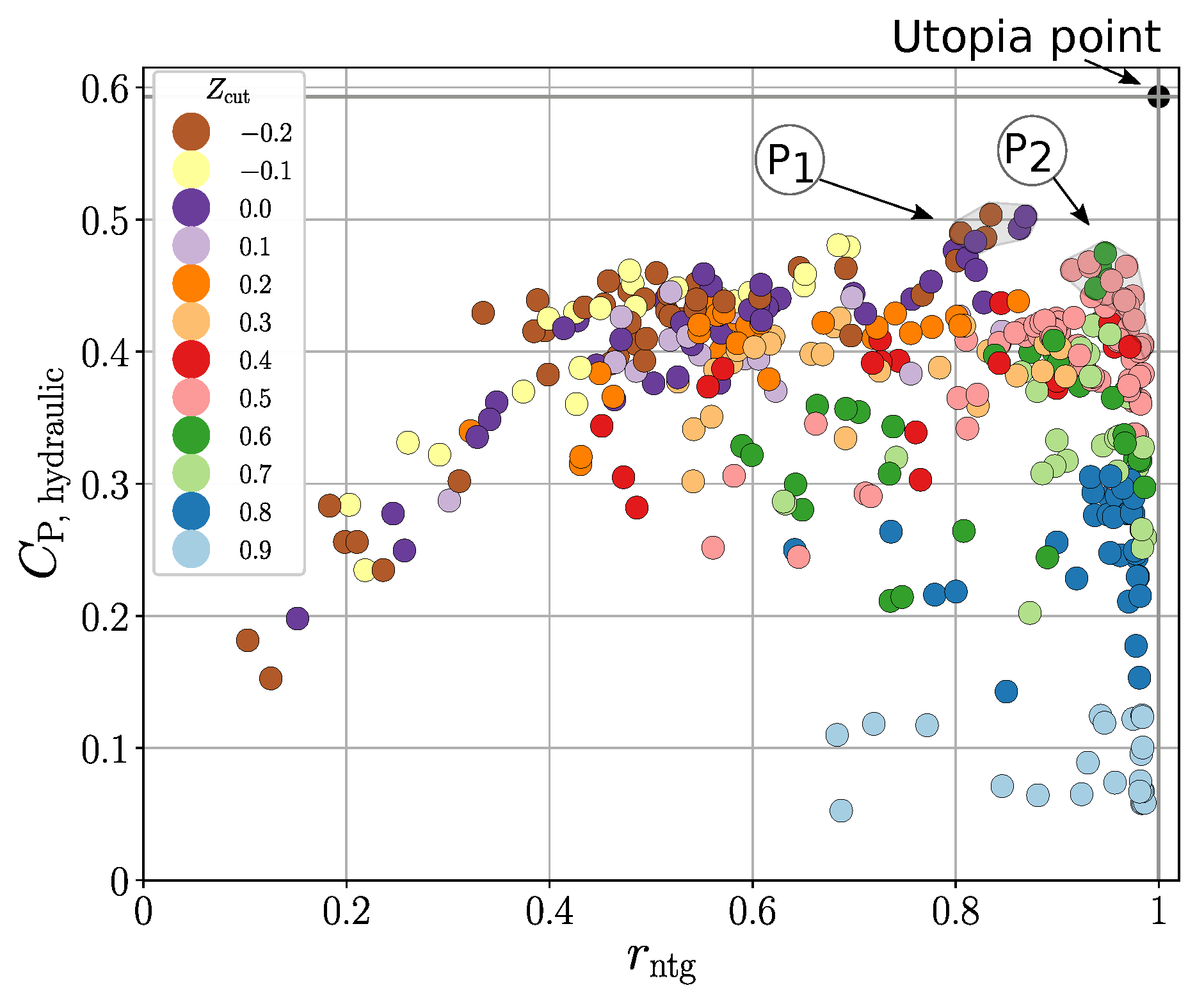
Before the performance of the Pareto-optimal individuals is further analysed, the dependence of individuals on the parameter
can be visualised; this is done in
Figure 5, where the data from
Figure 4 are shown coloured according to the values of
. Two groups of candidates, named as P1 and P2, were selected manually, based on their performance. Trends can be identified in the combination of input parameters possessed by each of these groups. Candidates from group P1 feature maximum
; in general, wheels of group P1 feature fewer, long, and inclined blades. By contrast, individuals from group P2 feature the maximum work ratio, and their blades are shorter, straighter, and in greater number. Wheels of group P1 and P2 are displayed in
Figure 6.
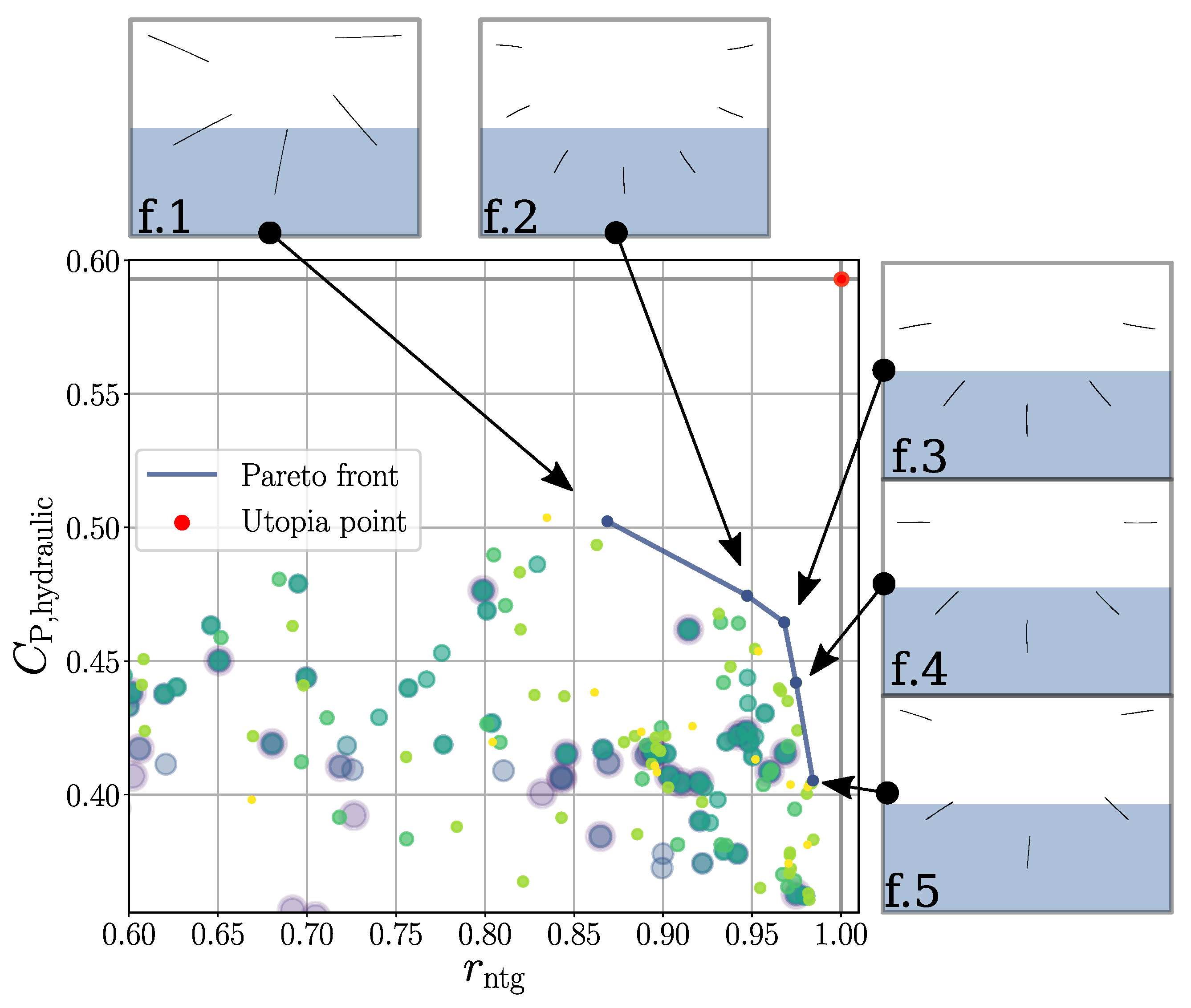
In the present case, the outer-most layer of individuals from the Pareto-optimal group was considered for further investigation. This Pareto front consists of five individuals (from here on designated f.1 to f.5), which are depicted together with their geometry in
Figure 7. There, the blue-shaded region represents an arbitrarily selected group of individuals of interest, and the scale of both axes is so that only high-performing individuals are shown. From here on, these five Pareto-optimal candidates are further investigated, in order to converge towards one optimal design.
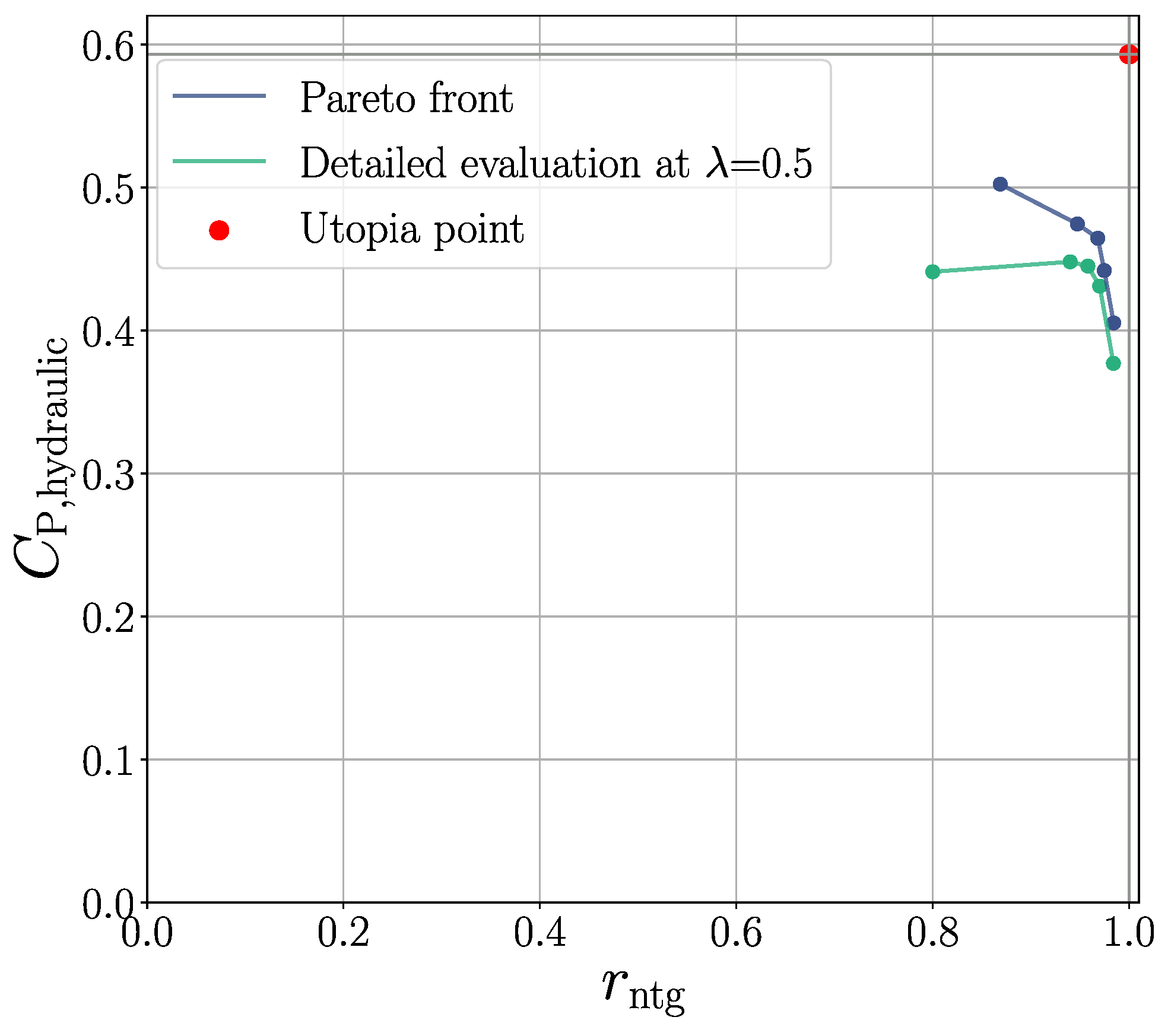
5.2. Detailed Evaluation of Top Candidates
During the optimisation, power values were extracted from
cfd simulations after 3
had elapsed (allowing the flow to settle down after initialisation) and until 15
had been simulated. In order to describe with even better accuracy the performance of the best candidates in the optimisation, an additional 3600
cpu-hours were invested by running these simulations over a longer duration of physical time. This methodology was developed earlier as a part of the water wheel optimisation in [
17]: first, the power output was ignored until five blades had entered and left the water. Then, the power was extracted during a duration corresponding to 15 blades passing through the water. Time intervals obtained in this way varied according to the number of blades for each design configuration; cases with fewer blades required a longer amount of physical time. Finally, the durations considered to analyse power extraction in this study ranged from 16 to 71
.
Once the power had been evaluated according to those criteria, the corresponding results (i.e., objective functions) were plotted along with the results of initial evaluations, as in
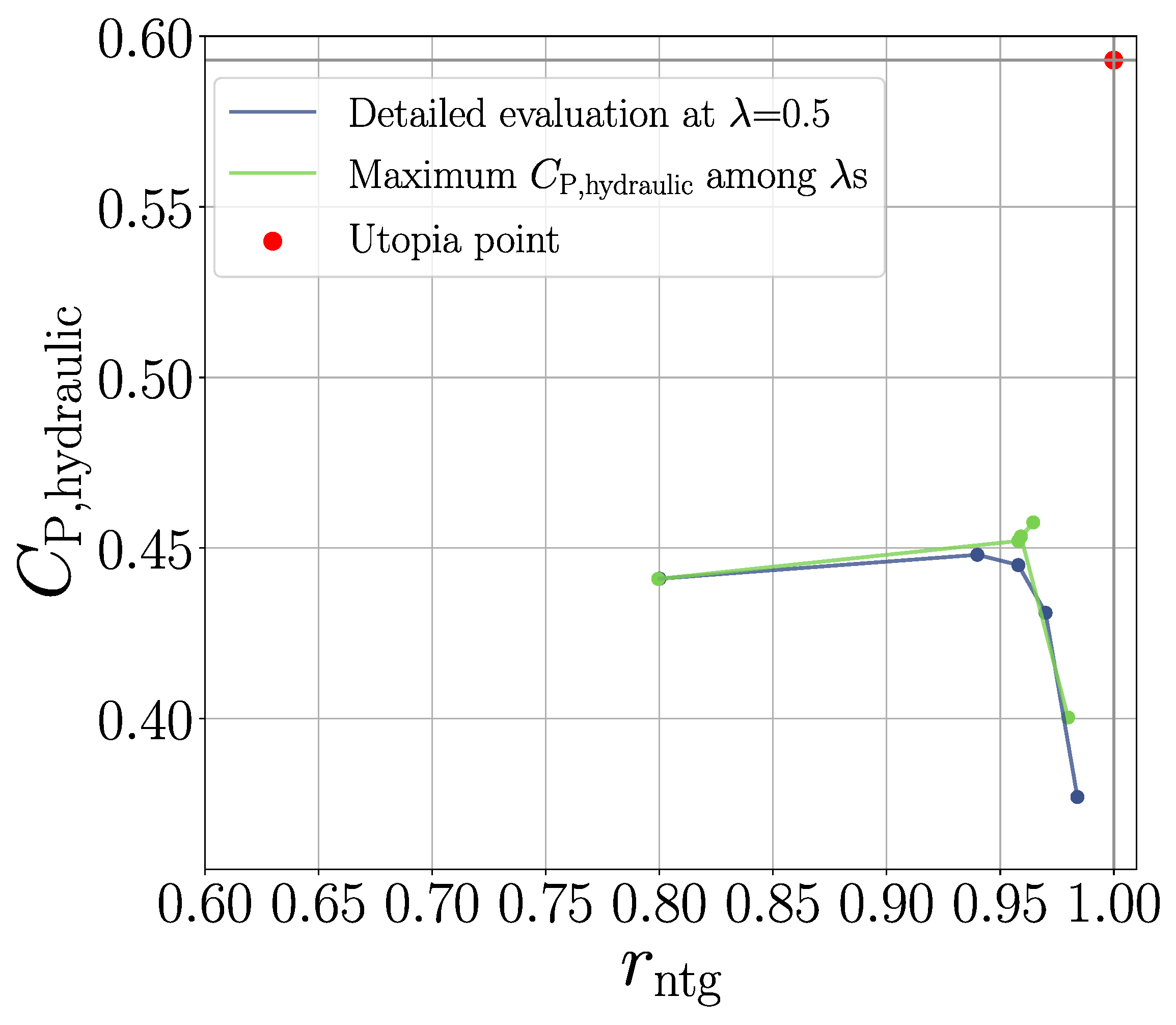
Figure 8, where blue and green dots indicate initial and detailed evaluations, respectively. It can be observed from this figure that the hydraulic power coefficient and work ratio decreased noticeably for all designs, particularly so for design f.1. The corresponding changes are listed in
Table 4. This detailed analysis reveals the lower robustness of the designs in group P1, maximising
; in that group, interactions with the free surface were very strong, with the formation of large waves and strong near-surface vortices, making accurate
cfd evaluations very challenging. On the other hand, changes in
were much smaller—down to 0—as seen in
Table 4. This means that an evaluation based on maximising
leads to robust designs, highlighting the superiority of group P2 for practical applications.
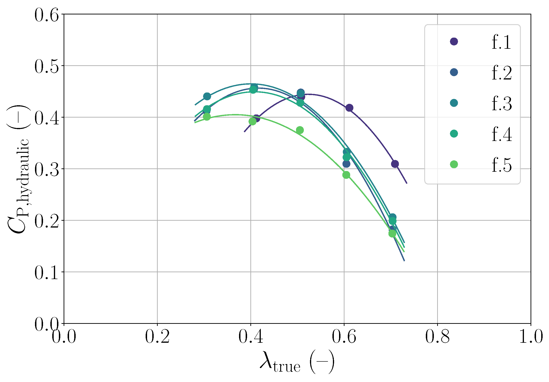
5.3. Optimum Tip-Speed Ratio
All evaluations carried out up to this point were configured with tip-speed ratio
. Further simulations of each of the five top-performing wheel configurations were then carried out with different values of the tip-speed ratio, in order to obtain power curves and identify the wheels’ optimum rotation speed. The experimental work carried out previously in the laboratory to validate the simulation model had already confirmed that this type of device produced maximum
at a tip-speed ratio near 0.5 [
16]. Thus, the range of studied tip-speed ratios was selected accordingly, i.e.,
[0.3, 0.7], in intervals of 0.1, translating into another 19 simulation cases carried out by investing an additional 15,000
cpu-hours. The obtained results are plotted in
Figure 9, where the
of these 19 configurations is plotted with respect to the tip-speed ratio.
From the results of these 19 simulations, the tip-speed ratio corresponding to the maximum
was selected for each of the five configurations. Both objective functions of these five designs are plotted in
Figure 10, along with the previously obtained performance values corresponding to
for comparison. Note that the scales do not start at zero, focusing on the high-efficiency region. An improvement in at least one objective function can be observed for wheels f.2 to f.5, whereas design case f.1 shows no improvement (as expected from observing
Figure 9, where it can be seen that the optimum tip-speed ratio is indeed 0.5). Remember that case f.1 has particularly long blades, with
.
The following key points can be made, based on this analysis of the Pareto-optimal group of wheels:
Wheels with longer blades have an optimum tip-speed ratio of 0.5, whereas wheels with short blades work most efficiently around .
Both extreme cases on the Pareto front (i.e., f.1 and f.5) could be discarded as these indicate lower performance compared to evaluations f.2 to f.4.
The remaining three best cases, i.e., f.2 to f.4, feature almost the same geometry, differing mainly by the number of blades. This could already be observed in
Figure 7, since parameter
has a very small influence on the geometry of short-bladed wheels.
5.4. Analysis of Best Evaluations
According to the method described earlier in
Section 2, building on top of former work [
16], the power stroke of each of these configurations, represented in a diagram showing
over the nondimensional stroke angle
, can be studied. Indeed, before discarding the two least-performing designs (f.1 and f.5) from the pool of best designs according to the results above, it is worth analysing the underlying power curves, as they give information about power production along the blade stroke, visualising and quantifying losses associated with blade entry and exit from the water, as well as interference between blades.
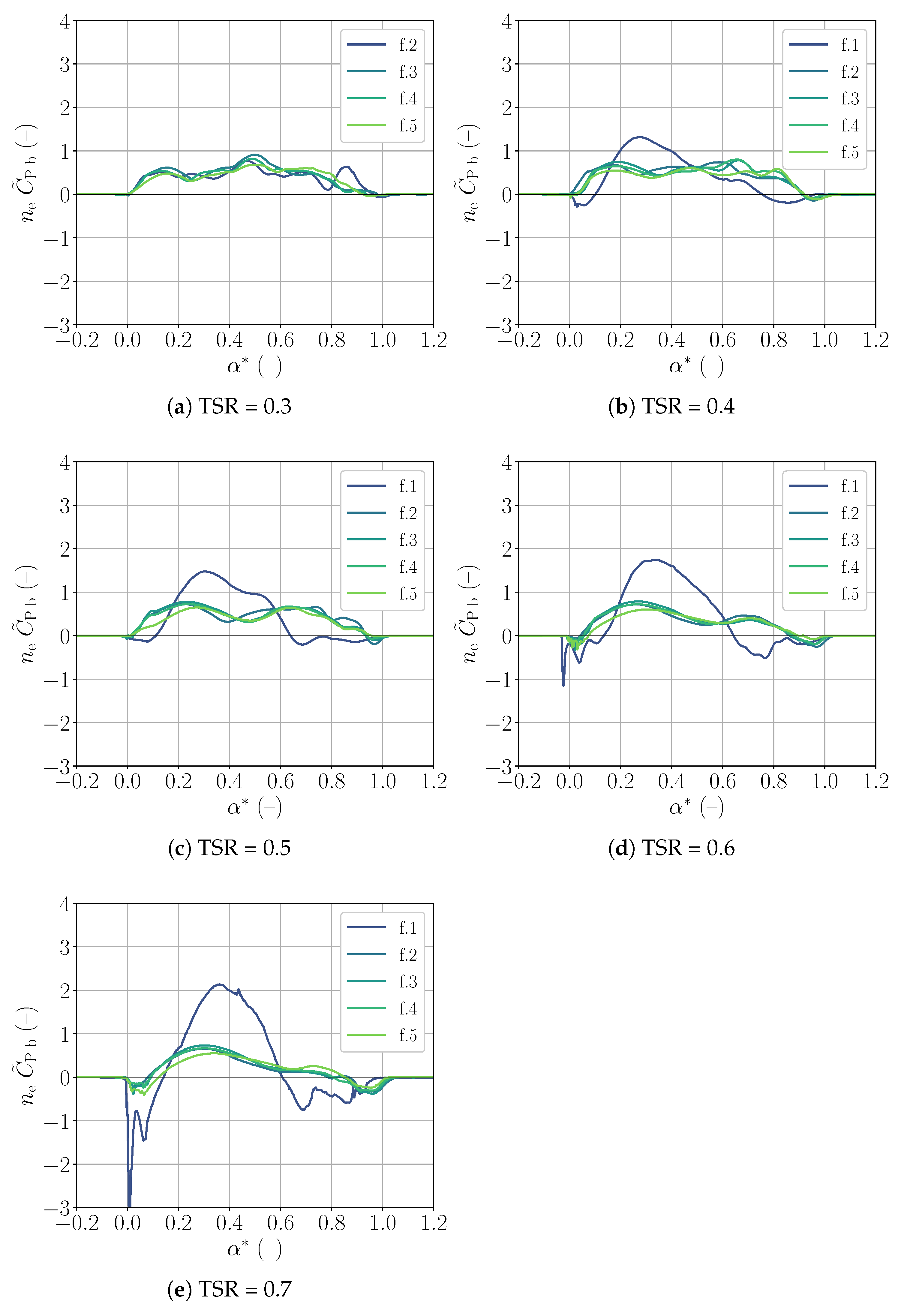
The corresponding plots are shown in
Figure 11 sorted according to the tip-speed ratio. In this figure, when
= 0, the tip of the blade crosses the horizon into the water; when
= 1, it crosses the horizon out of the water. The net area under any curve represents the time-averaged hydraulic power coefficient for the corresponding case. Positive values in these plots indicate zones where the blade is generating power (extracting energy from the water and transferring it to the shaft); negative values indicate zones where energy is lost by the blade into the water. This occurs for example when the blade splashes into or moves out of the water.
It can be observed from
Figure 11 that the power stroke curves of wheels f.2 to f.5 are largely similar. In contrast, for the f.1 water wheel, as visible from the dark blue line, the energy loss at the entry and exit is distinctly larger, and it increases with the tip-speed ratio. At the same time, the peak blade power is also largest for design f.1. Therefore, this particular wheel induces much stronger fluctuations on the generator shaft, which translates as structural stresses.
At their optimal tip-speed ratio (
Figure 11b), the wheels with short blades (i.e., f.2 to f.5) produced power for 92% of the stroke duration on average. Power is delivered in a regular manner, growing rapidly at first and then maintaining a value close to the mean power delivery up until late in the stroke. At the optimal rotation speed (
), power is delivered up until
= 0.9 (at which point the blade is 48
past the nadir point), when the blade is operating in the wake of two other blades further upstream. This is evidence that, as had been tentatively suggested in [
17], the optimum free-stream water wheel is clearly not a purely drag-based machine. The optimisation clearly indicates that for this radius and depth, wheels with fully immersed blades (
= 0.5) perform best, both from the point of view of net power output and the quality of mechanical power delivery.
Among the five wheels selected as part of the Pareto front, the three wheels f.2, f.3, and f.4 showed better performance compared to f.1 and f.5. Since those three wheels have a very similar geometry and performance, the configuration with the lowest number of blades was selected, reducing the construction cost and maximising simplicity, therefore, the wheel f.4 was designated as the optimal design in this study.
5.5. Comparison of Optimised Designs between Different Studies
A comparison of the best evaluations obtained in the present study with those obtained in our previous optimisation study [
17] is carried out below.
The previous optimisation study considered a much larger domain, with wheel diameters ranging from 0.4 to 6 in diameter, and 0.2 to 1 in depth; the work ratio was not considered. To address this very broad domain, a family of Pareto-optimal wheels (named “Magdeburg”) was proposed. Within this family, the design configuration corresponding to = 0.5 and R = (the same input parameters as those of the study presented here) was selected, in order to compare performance in the present study.
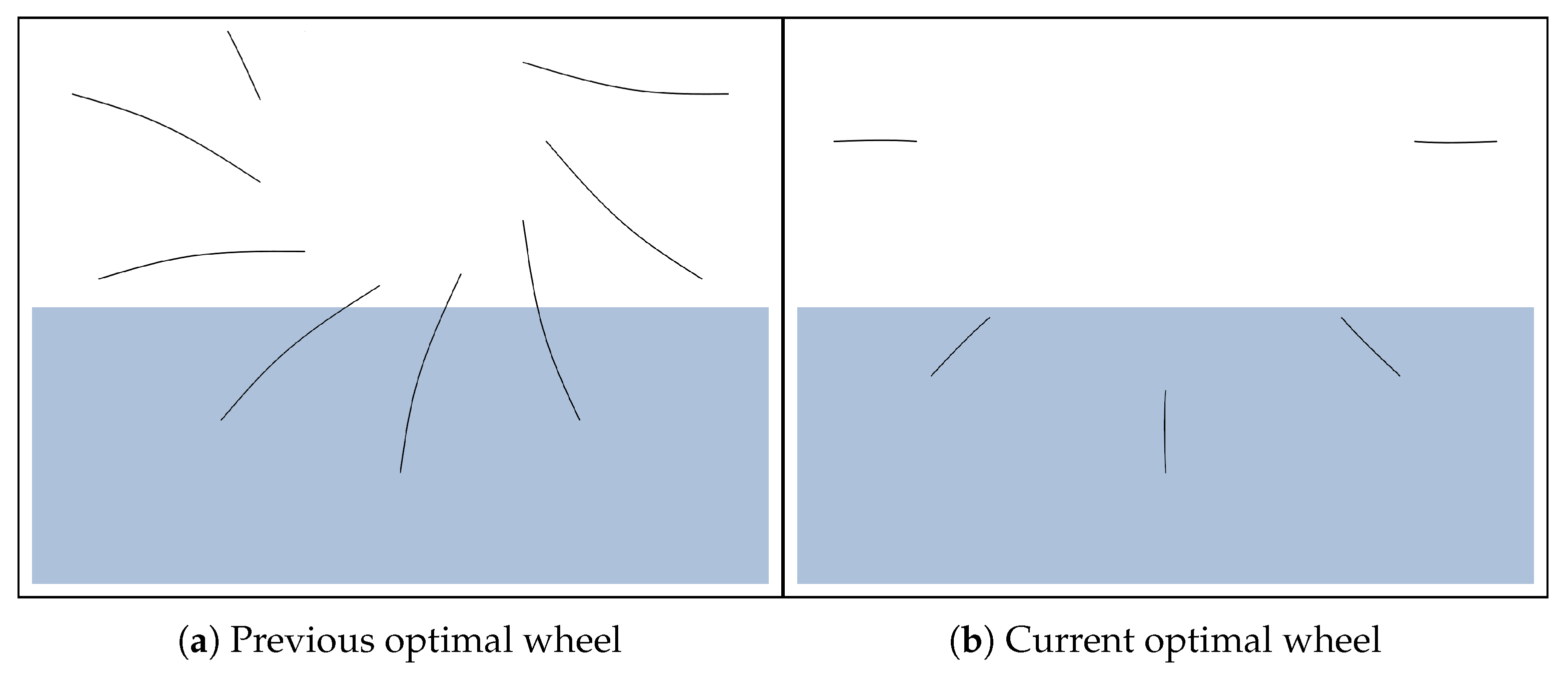
The geometries of the wheel selected from the previous optimisation study and of the optimal wheel from the current study are shown in
Figure 12. The previous study constrained the geometry so that the root of blades would remain above the water surface, while the current study finally recommends an immersed root blade.
The performance of each wheel was evaluated, with each operated at its respective optimum tip-speed ratio. The results of this comparison are presented in
Table 5.
It was observed that the work ratio of the optimised wheel obtained from the current study was 113% higher than the wheel suggested from the previous study. Moreover, the hydraulic- and rotor-based power coefficients were further improved by 8% and 8.2%, respectively. We note that this improvement in the power output has the same order of magnitude as the uncertainty associated with carrying out shorter evaluations during the optimisation proper, compared to more detailed evaluations (as visible in
Figure 8). Nevertheless, the improvement here is quantified by comparing two wheels with the same, rigorous method.
The total blade surface area per unit width for the current optimal wheel is /, which is 71% less than the area of the wheel proposed by the model in the previous study ( /). This translates into substantial material savings and will also lead to a reduction in production cost and structural weight.
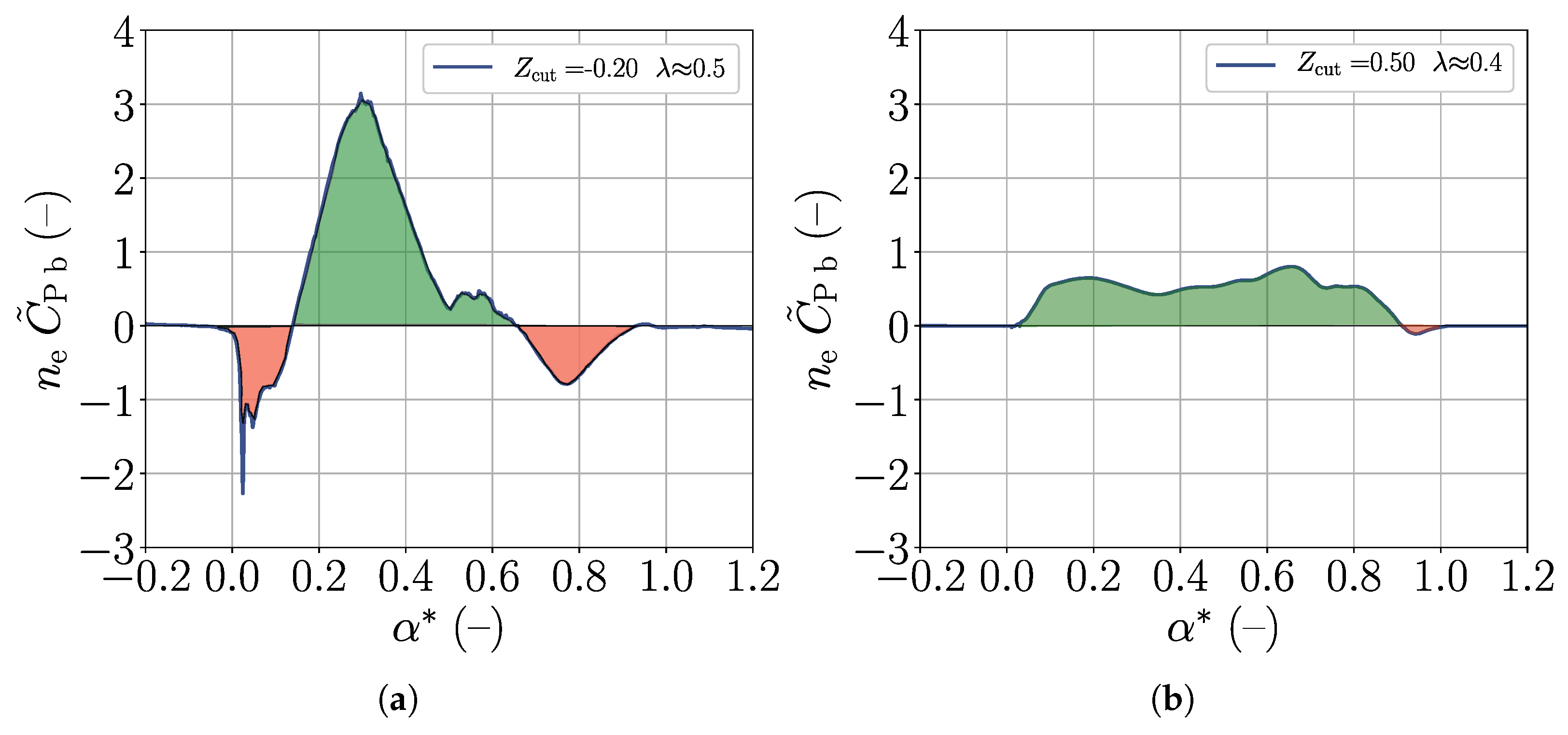
The performance of both wheels is compared in
Figure 13, using the approach described in
Section 2. In this figure, the green and red areas under the curve represent positive and negative contributions of power to the net hydraulic power, respectively.
It can be seen from
Figure 13a that in the wheel selected out of the previously proposed optimal family of designs, considerable energy loss occurs due to the entry splash and blade exit. These occur for
∈ [0–0.14] and
∈ [0.66–1]. The maximum torque occurs at around 40% of the stroke, and large oscillations in power delivery are observed, which is not desirable. By contrast, in the case of the current optimal wheel, in the current optimised wheel, losses become almost insignificant (
Figure 13b). Power is produced consistently between
values ranging from 0.01 to 0.92.
Thus, the concept of the immersed blade design is proven to be beneficial when maximising the performance of a free-stream water wheel with a radius of and a depth of , at least for the free-stream velocity of 1.2 m s−1 considered here. This suggests that the performance of wheel designs with other configurations may also be improved by increasing the blade root radius. This hypothesis is investigated in the following paragraphs.
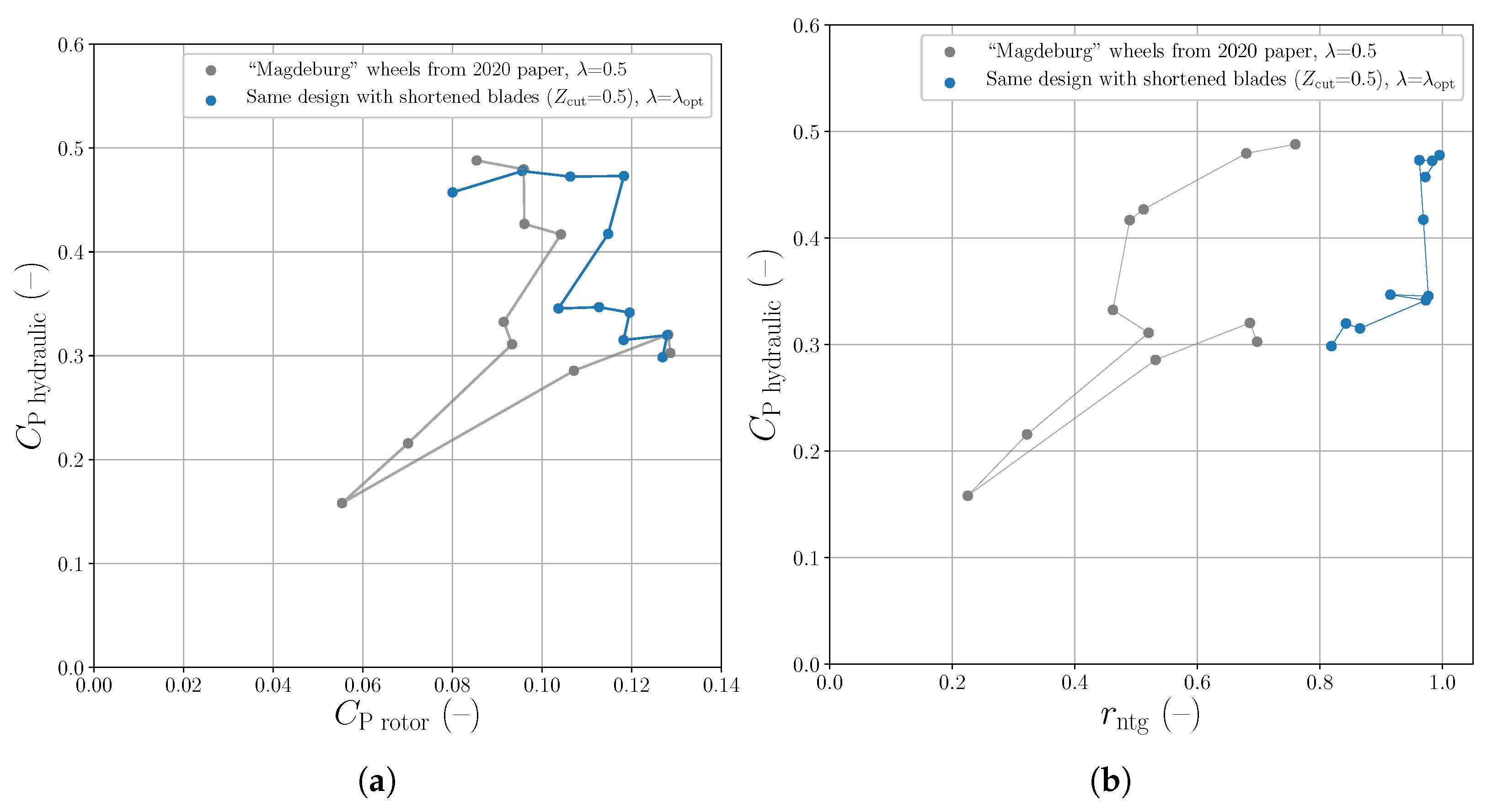
5.6. Revised “Magdeburg” Standard-Optimal Model
The previously published optimisation led to proposed design guidelines covering a wide range of designs, in an attempt to cover broadly the Pareto front that appeared when maximising simultaneously the pure hydraulic performance (measured using
) and the power density of the device (measured using
). Eleven wheel designs produced using those guidelines were then evaluated more thoroughly, revealing that their performance was not fully Pareto-optimal in this regard, especially for
values between 0.55 and 0.75. In light of the results obtained in the present work while studying a more restricted parameter range, results from the former optimisation were revisited. To this end, eleven wheels built according to the “
Magdeburg” guidelines were modified so that their blades were shortened with
= 0.5. The flow through each of those wheels was simulated for five values of
, and their performance was evaluated according to the detailed method described in
Section 2 above, consuming a total of 29,000
cpu-hours.
The results from this new evaluation are described in
Figure 14. In
Figure 14a, the vertical and horizontal axes display respectively the hydraulic and rotor power coefficients (the two objective functions that were to be maximised in [
17]). The grey dots are the wheels from the previous “Magdeburg” family, evaluated at
, as first presented in [
17]. The blue dots indicate the performance of the modified wheels–identical in all respects, except for their shortened blades—operated at their optimal tip-speed ratio (
for most wheels). In that figure, it is seen that for all but the largest and smallest wheels, the power output of the wheels is significantly increased when the blades’ size is reduced so that
= 0.5.
In
Figure 14b, the vertical axis again stands for the hydraulic power coefficient, but the horizontal axis represents the work ratio. The performance of the same wheels (from both the previous and the current study) is displayed using the same colour code. Since the work ratio was not considered as an objective function in the former optimisation, it is not a surprise that neither curve resembles a Pareto front. Nevertheless, the effect of shortening the blades is very clear: the work ratio of all wheels is drastically improved, with eight of the short-bladed wheels reaching
.
Those results make it unambiguous that reducing the length of the free-stream water wheel’s blades, so that the blades become fully immersed in the water during the power stroke, increases the performance of wheels with diameters and depths far below and above those of the wheel optimised in the present work. Even though this final investigation only identifies local optima, in the wait for a further optimisation, the guidelines published in [
17] are hereby updated to add
= 0.5 for every wheel.
6. Further Work
A potentially effective and relatively simple method for increasing the power output of the free-stream water wheel is to use a ducting device; optimal geometries for similar turbines have already been devised using numerical tools [
22,
23]. Work is under way that aims to identify an optimum deflector shape for the free-stream waterwheel using the very methods presented in the present article (
Figure 15).
Ultimately, the identification of the blade immersion fraction
as a significant design parameter in the present study calls for a new optimisation, in which this parameter would be added to the parameters varied in [
17] and which would search for geometries that maximise the hydraulic power coefficient, rotor power coefficient, and work ratio. This new optimisation, ranging again across a wide range of configurations, would ensure that optimal combinations of all input parameters (
,
,
,
,
R, and
) are attained all across the design space.
Lastly, the wheels’ performance ought to be studied with three-dimensional simulations, since the restriction to two dimensions is likely the largest methodological limitation of the current study. Although those are considerably more computationally expensive and do not currently allow for large-scale optimisations, the effect of flow in directions parallel to the wheel shaft, in particular on the power output, needs to be studied; this will be the subject of further research in the laboratory.
7. Conclusions
This numerical study of the free-stream water wheel, a low-density, low-impact hydropower device designed to operate at the surface of rivers, indicates that best performance is obtained with designs with fully immersed blades.
The present article expanded upon the work published in [
16,
17], in which robust two-dimensional numerical models for simulating and analysing free-stream water wheels were introduced. After the wheels’ geometry was parametrised to include a blade root immersion parameter, a genetic optimisation was carried out, varying blade pivot angles (
,
) and number of blades (
) while the tip-radius (
R) and wet radius fraction (
) remained fixed. The present study aimed to simultaneously maximise
and
, seeking for the best compromise between power production and the smoothness of power delivery.
After nearly 400 iterations obtained over three months, the optimiser converged towards a group of five Pareto-optimal designs. Extended post-processing and performance analysis of these allowed singling out an optimum design configuration (design f.4). A detailed comparison between the newly obtained optimum wheel and a comparable wheel extracted from the optimised family of designs in the previous study reveals the following:
The optimised wheel design, featuring fully immersed blades ( = 0.5) and the accordingly adapted blade geometry, results in a 113% increase in the work ratio, while still improving the hydraulic and rotor power coefficient by 8%, compared to the wheel suggested by the previously established design guidelines.
The recommended number of blades () and cut radius fraction () of the optimised design translate into a 71% reduction in total blade area, corresponding to significant reduction in weight, bulk, and material usage.
Applying the same geometrical modification to the complete set of wheel designs obtained in previously published studies reveals that performance is markedly improved in nearly every case, whether measured in terms of the hydraulic power coefficient, rotor power coefficient, or work ratio. In this manner, the two-dimensional study presented here, after 114,000 cpu-hours of computational time, unambiguously indicates that the optimal free-stream water wheel design has fully immersed blades, which produce power for most of the power stroke in a continuous fashion. This shows that lift, and not just drag, is also a primary energy conversion mechanism for those machines. Future work will make further use of the tools presented here in order to identify the optimal geometry for deflectors positioned upstream or below the wheel, as well as to study three-dimensional effects in the fluid flow and power dynamics of the free-stream water wheel.
Author Contributions
Conceptualisation, methodology, O.C.; writing—original draft preparation, A.S. and O.C.; software, investigation, validation, visualisation, A.S., O.C. and A.J.; writing—review and editing, A.S., O.C., A.J., S.H. and D.T.; supervision, project administration, funding acquisition, S.H. and D.T. All authors have read and agreed to the published version of the manuscript.
Funding
This work was initially supported by funding provided by the Fluss-Strom project financed by the Bundesministerium für Bildung und Forschung (German Federal Ministry of Education and Research) under Project Number 1714. One author benefited from the help of the Landeshauptkasse Sachsen-Anhalt.
Institutional Review Board Statement
Not applicable.
Informed Consent Statement
Not applicable.
Data Availability Statement
Not applicable.
Acknowledgments
The present work is partly based on the Master’s Thesis of the first author.
Conflicts of Interest
The authors declare no conflict of interest. The funders had no role in the design of the study; in the collection, analyses, or interpretation of the data; in the writing of the manuscript; nor in the decision to publish the results.
Nomenclature
| variable blade stroke angle () |
| nondimensional blade stroke angle, varies between 0 and 1 between horizon crossings (–) |
| blade angle at tip () |
| blade angle at pivot point () |
| mechanical shaft power developed by rotor () |
| tip-speed ratio (–) |
| optimal tip-speed ratio (–) |
| angular velocity of wheel () |
| density of water () |
| fixed blade stroke angle () |
| power coefficient of a single blade, averaged over several blades (–) |
| frontal area of wheel exposed to water () |
| total frontal area of wheel () |
| coefficient of power based on frontal immersed area in the water (–) |
| coefficient of power based on total frontal area of wheel (–) |
| wet radius fraction (–) |
| vertical distance of blade root from water surface () |
| depth of wheel in the water from water surface, positive downwards () |
| width of the blades () |
| number of blades (–) |
| effective number of blades (–) |
| R | tip-radius () |
| vertical distance of reference blade root from centre of wheel () |
| free-stream velocity () |
| work ratio (–) |
| cut radius fraction (–) |
References
- Müller, S.; Cleynen, O.; Hoerner, S.; Lichtenberg, N.; Thévenin, D. Numerical analysis of the compromise between power output and fish-friendliness in a vortex power plant. J. Ecohydraul. 2018, 3, 86–98. [Google Scholar] [CrossRef]
- Powalla, D.; Hoerner, S.; Cleynen, O.; Müller, N.; Stamm, J.; Thévenin, D. A computational fluid dynamics model for a water vortex power plant as platform for etho- and ecohydraulic research. Energies 2021, 14, 639. [Google Scholar] [CrossRef]
- Hoerner, S.; Kösters, I.; Vignal, L.; Cleynen, O.; Abbaszadeh, S.; Maître, T.; Thévenin, D. Cross-flow tidal turbines with highly flexible blades—Experimental flow field investigations at strong fluid–structure interactions. Energies 2021, 14, 797. [Google Scholar] [CrossRef]
- Hoerner, S.; Abbaszadeh, S.; Cleynen, O.; Bonamy, C.; Maître, T.; Thévenin, D. Passive flow control mechanisms with bioinspired flexible blades in cross-flow tidal turbines. Exp. Fluids 2021, 62, 104. [Google Scholar] [CrossRef]
- Müller, W. Die Wasserräder, 2nd ed.; Verlag Moritz Schäfer: Leipzig, Germany, 1939. [Google Scholar]
- Paudel, S. Experimental and Numerical Study of Dethridge Wheel for Pico-Scale Hydropower Generation. Ph.D. Thesis, Technische Universität Darmstadt, Department of Civil and Environmental Engineering, Darmstadt, Germany, 2016. [Google Scholar]
- Paudel, S.; Saenger, N. Dethridge wheel for pico-scale hydropower generation: An experimental and numerical study. In Proceedings of the 28th IAHR Symposium on Hydraulic Machinery (IOP Conference Series: Earth and Environmental Science), Grenoble, France, 2016; Volume 49, p. 102007. [Google Scholar]
- Quaranta, E.; Revelli, R. CFD simulations to optimize the blade design of water wheels. Drink. Water Eng. Sci. 2017, 10, 27. [Google Scholar] [CrossRef] [Green Version]
- Nguyen, M.H.; Jeong, H.; Yang, C. A study on flow fields and performance of water wheel turbine using experimental and numerical analyses. Sci. China Technol. Sci. 2018, 61, 464–474. [Google Scholar] [CrossRef]
- Quaranta, E.; Revelli, R. Hydraulic behavior and performance of breastshot water wheels for different numbers of blades. J. Hydraul. Eng. 2017, 143, 04016072. [Google Scholar] [CrossRef]
- Nishi, Y.; Inagaki, T.; Li, Y.; Omiya, R.; Hatano, K. Research on the flow field of undershot cross-flow water turbines using experiments and numerical analysis. In Proceedings of the 27th IAHR World Congress, Montreal, QC, Canada, 2014; Volume 22. [Google Scholar] [CrossRef]
- Nishi, Y.; Inagaki, T.; Li, Y.; Hatano, K. Study on an undershot cross-flow water turbine with straight blades. Int. J. Rotat. Mach. 2015, 2015, 817926. [Google Scholar] [CrossRef]
- Nishi, Y.; Hatano, K.; Inagaki, T. Study on performance and flow field of an undershot cross-flow water turbine comprising different number of blades. J. Therm. Sci. 2017, 26, 413–420. [Google Scholar] [CrossRef]
- Nishi, Y.; Hatano, K.; Okazaki, T.; Yahagi, Y.; Inagaki, T. Improvement of performance of undershot cross-flow water turbines based on shock loss reduction. Int. J. Fluid Mach. Syst. 2020, 13, 30–41. [Google Scholar] [CrossRef]
- Nishi, Y.; Yahagi, Y.; Okazaki, T.; Inagaki, T. Effect of flow rate on performance and flow field of an undershot cross-flow water turbine. Renew. Energy 2020, 149, 409–423. [Google Scholar] [CrossRef]
- Cleynen, O.; Kerikous, E.; Hoerner, S.; Thévenin, D. Characterization of the performance of a free-stream water wheel using computational fluid dynamics. Energy 2018, 165, 1392–1400. [Google Scholar] [CrossRef]
- Cleynen, O.; Engel, S.; Hoerner, S.; Thévenin, D. Optimal design for the free-stream water wheel: A two-dimensional study. Energy 2021, 214, 118880. [Google Scholar] [CrossRef]
- Quaranta, E. Stream water wheels as renewable energy supply in flowing water: Theoretical considerations, performance assessment and design recommendations. Energy Sustain. Dev. 2018, 45, 96–109. [Google Scholar] [CrossRef]
- Spiewack, M.W. Grundlastfähige Energiegewinnung Durch Ökologisch Verträgliche Flusswasserkraftanlagen; 2015. Available online: http://flussstrom.eu/ (accessed on 1 June 2021).
- Cleynen, O.; Hoerner, S.; Thévenin, D. Characterization of hydraulic power in free-stream installations. Int. J. Rotat. Mach. 2017, 2017. [Google Scholar] [CrossRef]
- Adams, B.M.; Bauman, L.; Bohnhoff, W.; Dalbey, K.; Ebeida, M.; Eddy, J.; Eldred, M.; Hough, P.; Hu, K.; Jakeman, J.; et al. Dakota, a Multilevel Parallel Object-Oriented Framework for Design Optimization, Parameter Estimation, Uncertainty Quantification, and Sensitivity Analysis: Version 6.10 User’s Manual (Sandia Technical Report SAND2014-4633); 2019. Available online: https://dakota.sandia.gov//sites/default/files/docs/6.10/Users-6.10.0.pdf (accessed on 21 April 2022).
- Mohamed, M.; Janiga, G.; Pap, E.; Thévenin, D. Optimal blade shape of a modified Savonius turbine using an obstacle shielding the returning blade. Energy Convers. Manag. 2011, 52, 236–242. [Google Scholar] [CrossRef]
- Kerikous, E.; Thévenin, D. Optimal shape and position of a thick deflector plate in front of a hydraulic Savonius turbine. Energy 2019, 189, 116157. [Google Scholar] [CrossRef]
Figure 1.
Schematic diagram of the parametrised water wheel geometry studied in this work, in which one blade is shown with a red thick spline (the number of blades is a variable in this study). This spline connects three points positioned using two angles
and
, as in the previously published optimisation [
17]. In this work, the altitude of those points is not modified, but the blade is “cut” (shortened) so that its root is located at a variable distance
from the horizon line. Water flows from left to right with free-stream velocity
, and the wheel rotates in the anti-clockwise direction with angular velocity
.
Figure 2.
Flow field from one simulation case in the optimisation, displaying the rotating polygonal mesh rotating relative to the fixed trimmed background mesh. Fine prism cells on the blade surfaces bring the average wall values down to below 1. Water flows from left to right, and air is above the water surface (red line). Colour denotes vorticity (with the colour scale saturated at ±24 s−1). The flow is shown after 15 have been simulated.
Figure 3.
Genetic algorithm flowchart, with the number of evaluations (designs) rejected, selected, and evaluated in each of the generations.
Figure 3.
Genetic algorithm flowchart, with the number of evaluations (designs) rejected, selected, and evaluated in each of the generations.
Figure 4.
Performance of all cases evaluated during the optimisation, coloured according to generation, with hydraulic power coefficient on the vertical axis and work ratio on the horizontal axis. A horizontal line at indicates the Betz limit.
Figure 4.
Performance of all cases evaluated during the optimisation, coloured according to generation, with hydraulic power coefficient on the vertical axis and work ratio on the horizontal axis. A horizontal line at indicates the Betz limit.
Figure 5.
Scatter plot of all 392 evaluations, colourised with respect to their cut radius fraction (). Two groups are identified manually, according to their performance and geometry. Group P1 features individuals with a relatively high hydraulic coefficient and also large blades (low values of ). In group P2, individuals have lower hydraulic coefficient and a higher work ratio; they also feature short blades (high values of ).
Figure 6.
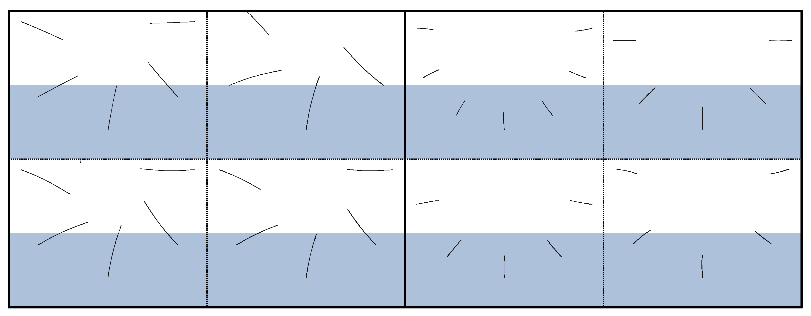
Geometries of water wheels from the broader Pareto front of the optimisation. Shown on the left are four geometries from group P1; on the right, four geometries are depicted from P2 group. In this figure, blade thickness is slightly exaggerated for a clearer representation.
Figure 6.
Geometries of water wheels from the broader Pareto front of the optimisation. Shown on the left are four geometries from group P1; on the right, four geometries are depicted from P2 group. In this figure, blade thickness is slightly exaggerated for a clearer representation.
Figure 7.
The top-5 best evaluations (Pareto front) of the optimisation, connected with a thick blue line. The respective geometries are also depicted. Dots indicate evaluations, with their colour and size indicating the generation they were produced in. The scales of both axes is such that only a portion of evaluated candidates are represented.
Figure 8.
Performance of the top-five designs (Pareto front) evaluated once with a standard duration of physical time (15
, as with all individuals during the optimisation) and once with thorougher criteria (as detailed in the text). The relative change in performance for all five configurations is detailed in
Table 4.
Figure 9.
The hydraulic power coefficient of the five Pareto-optimal candidates, plotted as a function of the tip-speed ratio . The line colours correspond to the design configurations described in the legend. The corresponding trend curves are plotted using 2nd-order polynomial best-fit models.
Figure 9.
The hydraulic power coefficient of the five Pareto-optimal candidates, plotted as a function of the tip-speed ratio . The line colours correspond to the design configurations described in the legend. The corresponding trend curves are plotted using 2nd-order polynomial best-fit models.
Figure 10.
Performance of the top-five (Pareto-optimal) individuals, selecting evaluations with maximum among different values of for each case. Note that the scales of both axes do not start at zero, focusing on the high-efficiency region.
Figure 10.
Performance of the top-five (Pareto-optimal) individuals, selecting evaluations with maximum among different values of for each case. Note that the scales of both axes do not start at zero, focusing on the high-efficiency region.
Figure 11.
Nondimensional blade power curves () as a function of nondimensional stroke angle () for the five Pareto-optimal wheels, plotted in separate diagrams for different tip-speed ratios. The part of the curves below the zero-line corresponds to energy transferred from the wheel to the water, which should obviously be avoided.
Figure 12.
Sketch of the geometry of the optimal wheel obtained from the previous optimisation study (top) and the optimal wheel from the current study (bottom), for the same radius and depth.
Figure 12.
Sketch of the geometry of the optimal wheel obtained from the previous optimisation study (top) and the optimal wheel from the current study (bottom), for the same radius and depth.
Figure 13.
Torque distribution represented by vs. curve for previous (top) and current (bottom) optimisation study. (a) Wheel selected from previous optimisation. (b) Optimal wheel from current study.
Figure 13.
Torque distribution represented by vs. curve for previous (top) and current (bottom) optimisation study. (a) Wheel selected from previous optimisation. (b) Optimal wheel from current study.
Figure 14.
Performance of wheels of the “Magdeburg” family of designs, constructed in previously published work [
17], compared to the same wheels modified with their blades shortened at
= 0.5. In those two series of simulations, the wheels range from 6
in diameter (wheels with the best
) down to
in diameter (wheels with best
). Part (
a) displays the wheels’ power output performance (hydraulic vs. rotor power coefficient), while part (
b) displays the wheels’ hydraulic power coefficient vs. work ratio
.
Figure 15.
A two-dimensional
cfd simulation based on the current work, also steered with a genetic optimiser, as part of the search for an optimal deflector shape to improve the power characteristics of the free-stream waterwheel. The colour scale and visualisation match those of
Figure 2.
Figure 15.
A two-dimensional
cfd simulation based on the current work, also steered with a genetic optimiser, as part of the search for an optimal deflector shape to improve the power characteristics of the free-stream waterwheel. The colour scale and visualisation match those of
Figure 2.
Table 1.
Numerical settings of reference simulation model used in this study. All settings are carried over from References [
16,
17], where they were discussed in greater detail.
Table 1.
Numerical settings of reference simulation model used in this study. All settings are carried over from References [
16,
17], where they were discussed in greater detail.
| software | Star-ccm+ (v14.04) |
| approach | 2D unsteady, segregated |
| meshing | rotating region: polygonal, |
| | non-rotating region: trimmed |
| mesh interface | overset |
| multiphase model | vof (air, water) |
| turbulence model | k-sst |
| boundary conditions | velocity inlet, slip walls top |
| | and bottom, mass-flow outlet |
| wall treatment on blades | all- wall treatment |
Table 2.
Range of input parameters for the present study, selected partly based on the results presented in [
17].
Table 2.
Range of input parameters for the present study, selected partly based on the results presented in [
17].
| Parameter | Range | Interval |
|---|
| Number of blades () | [6, 15] | 1 |
| Beta1 (), degrees | [0, 25] | 5 |
| Beta2 (), degrees | [10, 30] | 5 |
| Cut radius fraction () | [−0.2, 0.9] | 0.1 |
| Tip radius (R), m | 1.8 | – |
| Wet radius fraction () | 0.5 | – |
Table 3.
Genetic algorithm settings used to control Dakota’s moga algorithm for each of the three phases of the optimisation.
Table 3.
Genetic algorithm settings used to control Dakota’s moga algorithm for each of the three phases of the optimisation.
| Criteria | Phase 1 | Phase 2 | Phase 3 |
|---|
| crossover_type | shuffle random |
| num_parents | 2 | 3 | 3 |
| num_offspring | 2 | 3 | 3 |
| crossover_rate | 0.5 | 0.7 | 0.65 |
| mutation_type | offset normal |
| mutation_scale | 0.2 | 0.4 | 0.2 |
| mutation_rate | 0.5 | 0.75 | 0.5 |
| fitness_type | layer rank |
| replacement_type | below limit = 5 |
| shrinkage_fraction | 0.75 | 0.75 | 0.75 |
Table 4.
Change in the performance (value of objective functions) of the five top-performing individuals after a detailed evaluation was performed.
Table 4.
Change in the performance (value of objective functions) of the five top-performing individuals after a detailed evaluation was performed.
| Wheel Id | | |
|---|
| f.1 | −0.061 (−12.2%) | −0.069 (−7.8%) |
| f.2 | −0.026 (−5.5%) | −0.007 (−0.7%) |
| f.3 | −0.019 (−4.1%) | −0.010 (−1%) |
| f.4 | −0.011 (−2.5%) | −0.005 (−0.5%) |
| f.5 | −0.028 (−6.9%) | 0.000 (0%) |
Table 5.
On the left, one design among a family of optimal designs obtained in the previous optimisation study [
17], selected because its radius matches that of the current study. On the right, the optimum designed obtained in the current optimisation study. The performance of both wheels is evaluated at their optimum tip-speed ratio.
| Wheel Selected Out of Previous Optimisation | Current Optimal Wheel, Design f.4 |
|---|
| Input variables | Input variables |
| = 11 | = 8 |
| = 10 | = 0 |
| = 25 | = 10 |
| = −0.2 | = 0.5 |
| = 0.5 | = 0.4 |
| Objective functions | Objective functions |
| = 0.42 | = 0.45 |
| = 0.10 | = 0.11 |
| = 0.45 | = 0.96 |
| Publisher’s Note: MDPI stays neutral with regard to jurisdictional claims in published maps and institutional affiliations. |
© 2022 by the authors. Licensee MDPI, Basel, Switzerland. This article is an open access article distributed under the terms and conditions of the Creative Commons Attribution (CC BY) license (https://creativecommons.org/licenses/by/4.0/).


