Relevance of Optimized Low-Scale Green H₂ Systems in a French Context: Two Case Studies

Abstract

Hydrogen has been identified as a very promising vector for energy storage, especially for heavy mobility applications. For this reason, France is making significant investments in this field, and use cases need to be evaluated as they are sprouting. In this paper, the relevance of H${}_2$ in two storage applications is studied: a domestic renewable electricity production system connected to the grid and a collective hydrogen production for the daily bus refill. The investigation consists of the sizing of the system and then the evaluation of its performance according to several criteria depending on case. Optimizations are made using Bayesian and gradient-based methods. Several variations around a central case are explored for both cases to give insights on the impact of the different parameters (location, pricing, objective, etc.) on the performance of the system.Our results show that domestic power-to-power applications (case 1) do not seem to be competitive with electrochemical storage. Meanwhile, without any subsidies or incentives, such configuration does not allow prosumers to save money (+16% spendings compared to non-equipped dwelling). It remains interesting when self-sufficiency is the main objective (up to 68% of energy is not exchanged). The power-to-gas application (case 2, central case), with a direct use of hydrogen for mobility, seems to be more relevant according to our case study, we could reach a production cost of green H${}_2$ around 5 €/kg, similar to the 3–10 $/kg found in literature, for 182 houses involved. In both cases, H${}_2$ follows a yearly cycle, charging in summer and discharging in winter (long term storage) due to low conversion efficiency.

1. Introduction

1.1. Context

Energy storage is one of the key technologies that allow (or will allow) a better use of energy resources, and in particular will allow the solving of the problems linked to the integration of renewable resources, which are by nature variable in time [1,2,3,4]. In simple terms, the problem is to satisfy an energy need at a given moment and at a given point, from sources that vary in time and are spread over a territory. The link between these two actors is called a “grid”, which becomes a “smart-grid” when specific functions are added to [1]. It is thus possible to manage production, by starting or stopping certain devices that support it (hydraulic energy, gas power station, for example). One can also manage demand by favoring or penalizing the use of energy at certain times (mainly via the price signal), or even by taking control of equipment, by Direct Load Control (DLC) and Demand-Side Management (DSM). However, the most flexible way to achieve this adaptation is to use the storage device [5,6,7]. Unfortunately, storage almost systematically involves energy dissipation related to the necessary conversions, as well as for some forms of storage, a loss of capacity over time. Thus, because of these non-idealities, the implementation of a storage system must be carefully considered and analyzed, over time, in terms of energy and economy at least. The environmental aspects, over the complete life cycle of the device, must also be taken into consideration. Thus, associated with the cost of installation, storage systems—whatever their nature—must be designed and operated to achieve maximum performance. Thus, the scientific literature abounds [5,8,9,10,11,12,13] and much of it focuses on the expected behavior and performance of a storage system. When focusing on systems adapted to the residential sector, one must consider small capacity and diffuse systems. These residential micro-smart-grids—or smart-storage—have several singular characteristics. Thus, one generally converges to an electrical energy production system (often PV, sometimes wind) whose production is oriented towards self-consumption. The power calls are generally very variable because they do not benefit from the “averaging” effects due to the multiplicity of consumers. The very structure of the system can be variable over time, the classic example being the electric vehicle, which extends the storage capacity but whose presence is not continuous and difficult to predict. Finally, the residential sector raises issues of space, but also of equipment safety and maintenance. For these reasons, we limit the renewable energy source to photovoltaic cells and do not incorporate in this study wind turbines or concentrated solar systems that are better suited for bigger installations [14,15,16].

1.2. Literature Review

In [17], the authors study the performance of a system with PV, battery storage (stationary and from electrical vehicles), and access to the main-grid. They propose and evaluate an energy management strategy by incorporating the notion of non-critical load which presents tolerances on their operating domain (voltage may be 20% below the nominal value). This equipment thus provides an additional degree of freedom to the algorithm for minimizing the demand on the grid. Note here (again) that the system, the consumptions, and the PV production are perfectly defined (including vehicle presence/kilometre and non-critical load scheduling). However, the authors show an overall reduction of the grid call (thus an increase of the self-consumption share) and a 50% reduction of the peak power demand. In [18], an analysis of the main simulation/optimization tools are available, with a prevalence of the Homer tool should it be for a standalone system [19,20,21], a network of small systems [22,23], or for facilities [24,25,26,27,28]. From an economic point of view, Zakeri et al. [29] show that financial mechanisms encouraging self-consumption (instead of reinjection) would be relevant. They announce a savings of 41 to 74% for a combined storage/PV system. More generally, Ref. [30] presents a review of the literature on the economic benefits of microgrids. They conclude that there is potentially a substantial economic gain, while insisting that the monetization strategy must be adapted to the specificities of the deployment site. The literature incorporating a hydrogen storage is also very abundant [13,31,32,33,34]. In [35], the authors present an Energy Management System (EMS) adapted to a smart autonomous electrical grid (SAEG) connecting production resources (controllable: Diesel Generator and not controllable: Wind Turbine, PV) and consumers (which can be reactive so consumption can be shifted, or not). The storage is constituted by a couple electrolyzer/fuel cell, the H${}_2$ being stored in gaseous form in a tank, as well as the battery of the electric vehicles present in some dwellings. The objective function has three sub-objectives: (1) minimization of the operational cost, (2) maximization of the reliability, and (3) reduction of the unsatisfied (for the reactive consumers, the difference between the desired consumption, and the energy actually supplied). The minimization is performed using a shuffled frog leaping algorithm (SFLA). They show that the presence of storage facilities improves sub-objects 1 and 2 but tends to increase the rebound effect driven by insatiability. This raises the question of the weighting of the sub-objectives to build the global objective function, and thus the influence of this choice on the “optimal” solution obtained. In Ref. [36], an optimization of a mini-grid integrating PV, battery and hydrogen, in an insular context is presented, where, despite the presence of a main grid, energy autonomy is desired. Thus, the objective function integrates the maximization of the financial efficiency and the minimization of the grid call. The authors conclude about the need to develop design tools, requiring a precise description of the application case (available resources and consumption). Then, Ref. [37] presents a micro-grid including a wind turbine, a hydrogen storage, and a battery storage through an electric vehicle. As the installation actually exists, the results of modelling are compared to measurements (average error less than 2%). Finally, Ref. [38] presents a comparison of the performance of an isolated micro-grid (PV, batteries and H${}_2$) according to two strategies. The first one is qualified as “myopic control” in the sense that only the present state is taken into consideration to make decisions. The second approach implements a prediction of the production and consumption over a future time horizon of 12 h in order to refine the control strategy. However, the authors remain unclear on the method used to obtain these predictions.

1.3. Contributions to Novelty

With the global trend gearing for energy storage technologies, and public investment soaring on those technologies, as France with its “France relance” [39] plan, the relevance of those technologies should be evaluated for usage by a private individual connected to the national grid, as they could be important users of those technologies. Meanwhile, the concrete applications of H${}_2$ energy vector are not that clear in the French context. Thus, this work proposes to study the relevance of using one or two energy storage technologies, electrochemical batteries and gaseous hydrogen systems under three different French climates and different energy allocation strategies (self-sufficient, economic), exogenous conditions (price raise, transit cost) and configurations (number of dwellings, rooftop coverage). First, a Power-to-Power (P2P) paradigm is studied, before moving to a Power-to-Gaz (P2G) paradigm, before concluding on the usage of those technologies and how to enhance them.

Even if a software was developed specifically for this study, we believe that the main contributions to novelty of this article revolve around the assessment of these two case studies within the French context.

2. Methodology

2.1. Algorithm Architecture

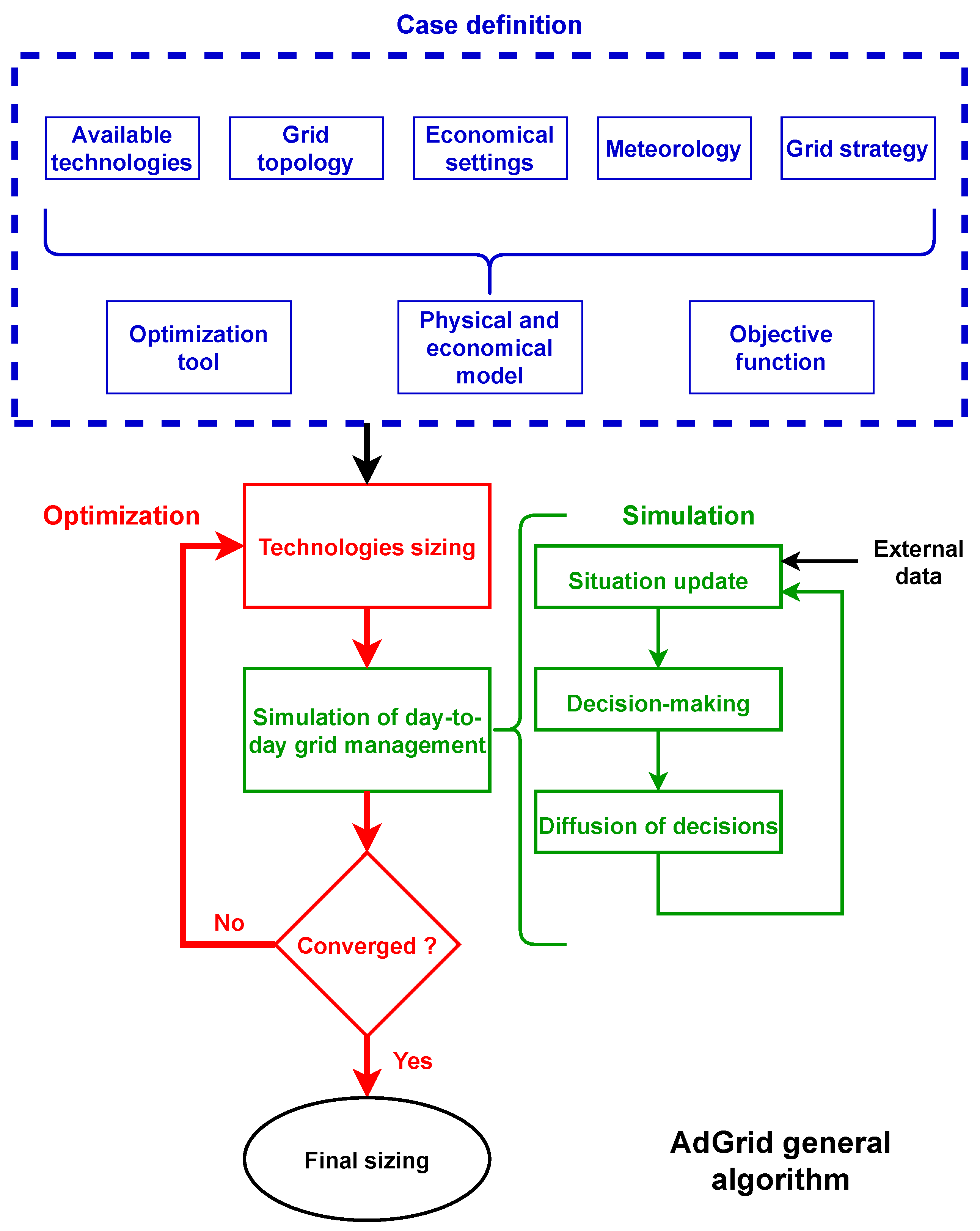
A proprietary code, written in Python 3.8, was developed for this study. It is object-oriented and separates into three parts: case definition, simulation and optimization (Figure 1).

In the “case definition” part, the various pieces of equipment of the energy chain and how they are connected to each other are defined, the meteorological conditions, the objective function (economic, independence, maximum consumption…) as well as the optimization tool (genetic algorithm, particle swarm optimization, Bayesian, Levenberg–Marquardt…) and the energy allocation strategy.

The “simulation” part assembles the various components following the defined topology and runs the model accordingly to the energy allocation strategy. A time step of 1 h will be used so as to not have to take into account the transitory phases.

Regarding the “optimization” part, its role is to manage the optimization schema of the simulations using the instruction of the user.

Such an architecture enables easily changing configuration.

2.2. Physical Model

2.2.1. PhotovoltaïCs

The PV panel model is based on [40]. In this model, the electrical power produced $P_{PV}$ [$\mathrm{W}$] is directly proportional to the received irradiation (global irradiation I [$\mathrm{W} {\mathrm{m}}^{-2}$] in the collector panel) and to the collector area, this latter being equal to 2 m${}^2$. The number of PV panels is noted $N_{PV}$. The proportionality coefficient, ${\eta }_{PV}$, which corresponds to the overall conversion efficiency of the photovoltaic chain, takes into account phenomena intrinsic to photovoltaic conversion (intrinsic conversion efficiency and its decrease with temperature), inverter/MPPT efficiencies, losses in cables, etc.

The efficiency is assumed to decrease linearly (coefficient $\alpha >0$ [${\mathrm{K}}^{-1}$]) above a reference temperature (which corresponds to the standard test conditions STC: 25 ${}^{\circ }\mathrm{C}$ and 1000 $\mathrm{W} {\mathrm{m}}^{-2}$) and $T_{PV}\left(t\right)$ [${}^{\circ }\mathrm{C}$] the operating temperature of the panel, which depends on the ambient temperature $T_{\infty }\left(t\right)$ and the irradiation:

$$\begin{array}{c}\hfill T_{PV}\left(t\right)=T_{\infty }\left(t\right)+\left({\displaystyle \frac{NOCT-20}{800}}\right)·I\left(t\right)\end{array}$$

(1a)

$$\begin{array}{c}\hfill P_{PV}\left(t\right)={\eta }_{PV,conv}·N_{PV}·P_{PV,STC}·\left[{\displaystyle \frac{I\left(t\right)}{1000}}·\left(1-\alpha ·(T_{PV}\left(t\right)-25)\right)\right]\end{array}$$

(1b)

The NOCT (Normal Operating Cell Temperature) is the equilibrium temperature of a panel placed in an atmosphere at 20 ${}^{\circ }\mathrm{C}$ and subjected to a flow of 800 m².

The PV panel’s max power per house was computed with geometrical considerations. In order to calculate the area available $A_{av.}$, a house of 7 × 10 m${}^2$ was chosen, $A_h$ with a roof angle $\theta$ of $\frac{\pi }{4}$, where only the best half of the roof can be covered. It gives 50 m${}^2$ of area available, corresponding to a maximum of 17 kW/house, as the irradiation peak, $I_{max}$, is equal to 360 W$·$m${}^{-2}$:

$$\begin{array}{c}\hfill A_{av.}=0.5·\frac{A_h}{cos\left(\theta \right)}=50{\mathrm{m}}^2\end{array}$$

(2a)

$$\begin{array}{c}\hfill P_{peak}^{PV}=A_{av.}·I_{max}=17\mathrm{kW}/\mathrm{house}\end{array}$$

(2b)

2.2.2. Electrolyzer and Fuel Cell

A static efficiency was used for both the electrolyzer and the fuel cell. These efficiencies, ${\eta }_{el}$${\eta }_{fc}$, contain all the information useful to build a simplified model of the behavior of an electrolyzer. This approach also allows us to take into account the auxiliary energy consumption associated with the control and regulation systems, but also, when integrated in the electrolyzer apparatus, to the compression stage.

The energy efficiencies are defined from a system point of view, with respect to the Higher Heating Value of hydrogen ($HHV=286\mathrm{kJ} {\mathrm{mol}}^{-1}=141.86\times {10}^6\mathrm{J} {\mathrm{kg}}^{-1}$) for the fuel cell and the Lower Heating Value ($LHV=242.7\mathrm{kJ} {\mathrm{mol}}^{-1}=120.38\times {10}^6\mathrm{J} {\mathrm{kg}}^{-1}$) for the electrolyser, as made by [33]:

$$\begin{array}{c}\hfill {\eta }_{el}={\displaystyle \frac{{\dot{m}}_{el}·HHV}{P_{el}}}\end{array}$$

(3a)

$$\begin{array}{c}\hfill {\eta }_{fc}={\displaystyle \frac{P_{fc}}{{\dot{m}}_{{\mathrm{H}}_2,fc}·LHV}}\end{array}$$

(3b)

2.2.3. Hydrogen Storage

The storage of hydrogen in the energy context is done either in pure form under pressure in the gaseous state, or in the form of metal hydride [41,42,43].

It is considered here that the H${}_2$ is stored under pressure in a tank with a static volume $V^{tank}$ and temperature $T^{tank}$ and a pressure $p^{tank}\left(t\right)$ [44,45]. A virial equation was used as the equation of state for the H${}_2$ stored. Compressibility factor Z was calculated with data taken from [46]. It has been validated up to 1000 bar and up to 473 K. Moreover, as H${}_2$ is used as a fuel, the energy in the tank is the product of the mass and of the Higher Heating Value (HHV). Thus:

$$E^{tank}\left(t\right)=Z(p,T)·\frac{p^{tank}\left(t\right)·V^{tank}·M^{{\mathrm{H}}_2}·HHV}{R·T^{tank}}$$

(4)

It is also considered that the max charging and discharging rate of the tank are, in practice, respectively limited by the electrolyzer and the fuel cell limits.

2.2.4. Battery

Electrochemical storage [47] is modeled here by considering a homogeneous set of individual batteries regarded as a single battery of capacity $C_{nom}^{bat}$ whose charge ($C^{bat}\left(t\right)$) evolves at each time step $\mathsf{\Delta }t$ as a function of the charge power, $P_{in}^{bat}$, and discharge power, $P_{out}^{bat}$). This results in the following first law based equation:

$$C^{bat}(t+\mathsf{\Delta }t)=C^{bat}\left(t\right)+{\eta }^{bat}(P_{in}^{bat}+P_{out}^{bat})·\mathsf{\Delta }t$$

(5)

where ${\eta }^{bat}$ is the battery charging and discharging efficiency.

The maximum value of the stored energy $C^{bat}\left(t\right)$ is limited by the nominal capacity $C_{nom}^{bat}$. Regarding the minimum value, a lower limit $C_{min}^{bat}$ below which the battery risks being deteriorated because of irreversible phenomena is introduced [48,49].

2.2.5. Converter

Electrical converters are necessary to adapt the nature of the electricity (DC/AC) as well as the voltage levels. They are modeled with a static efficiency, ${\eta }^{conv}$, and the input power, $P_{max,in}^{conv}$:

$$P_{out}^{conv}={\eta }^{conv}·P_{in}^{conv}$$

(6)

The output power is also limited to $P_{max,out}^{conv}$.

Some authors [50] introduce a variation of the efficiency for low powers in order to take into account the decrease of efficiency when the equipment operates far from the nominal regime.

2.3. Input Data

2.3.1. Meteorology

Two meteorological measures are needed to compute the production of PV panels: temperature and irradiation. They are both taken from the PVGIS database [51], a free European meteorological database giving years-averaged values. The values used correspond to the city of Pau, in France (oceanic climate).

2.3.2. Energy Tariffs

Energy tariffs are based on historical intraday prices values for France (and thus Western Europe, due to the European Power EXchange [52]), following a Real-Time Pricing (RTP) logic. Price of the energy bought to the grid is different from the price of the energy sold to it. It is considered that the former is equal to the RTP, while the latter is set equal to three times the RTP values, as it is the proportion observed between the cost of electricity for retailers and for consumers because of taxes and distribution costs, according to a report of the French competition authority [53].

2.3.3. Load

The load is aggregated. It corresponds to a house heated by electricity. The shape was extracted from the IHOGA software [54]. Then, this shape is scaled to fit the energy consumed in France by a dwelling, according to public data given by ENGIE (french gas and electricity provider) for consumption in France [55,56].

2.4. Equipment Settings

Table 1. Economic settings of the equipment.

Name	CAPEX	OPEX (% of the CAPEX)	References
Battery	792.2 €/kWh	2	[57]
Converter	neglected	neglected	[33]
Electrolyzer ${}^1$	3947 €/kW	2	[58]
Fuel cell ${}^1$	4600 €/kW	2	[59]
Fuel tank	470 €/kg	2	[60]
PV panels	1547 €/kW	1.5	[32]

¹ The evolution of the CAPEX of the electrolyzer and fuel cell are not linear but are corrected in a power law as recommended in [33,61]

summarizes the different values of CAPEX and OPEX for the different equipment. CAPEX represents the initial investment cost while OPEX corresponds to maintenance and replacement costs, but not the cost of the electricity or H${}_2$ consumed. Neither capital cost nor incentives or subsidies are considered.

Table 2. Technical settings of the equipment.

Component	Variable	Value	Reference
Battery	Degradation rate	7.12 $\times {10}^{-5}$ (-)	[62]
	Efficiency (charge and discharge)	0.95 (-)	[33]
Converter	Efficiency	0.95 (-)	[50]
Electrolyzer	Efficiency	0.7 (-)	[63]
Fuel cell	Efficiency	0.5 (-)	[63]
Fuel tank	Pressure	10 (bar)	N/A
	minimum
	Pressure	fist case: 100 (bar)	N/A
	maximum	second case: 700 (bar)
	Temperature	55 (°C)	[63]
PV panels	Temperature coefficient ($\alpha$)	$3.4\times {10}^{-3}$	[64] & datasheets
	NOCT	43 (°C)	datasheets
	Auxiliary systems efficiency ${}^{☆}$	0.8	N/A

${}^{☆}$ mainly inverter, MPPT and wiring.

presents the technical settings taken for the different equipment. Concerning the fuel tank, minimum and maximum pressure for the tank have been chosen in a range commonly used for compressed H${}_2$ storage, according to [60] and are different, as the scale is different between the first and the second case.

3. First Case Study: Domestic Power-to-Power Hydrogen

3.1. Case Description

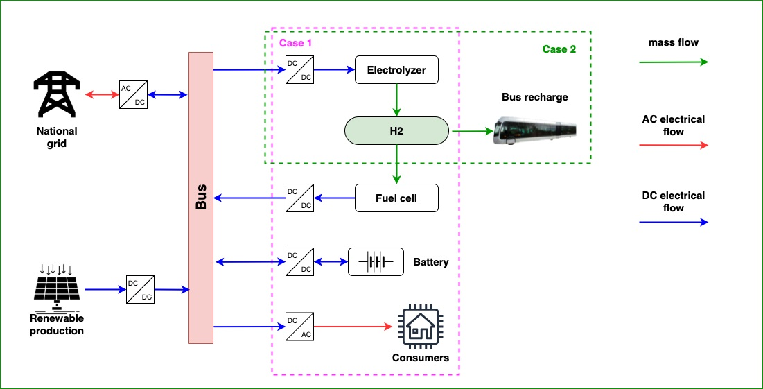
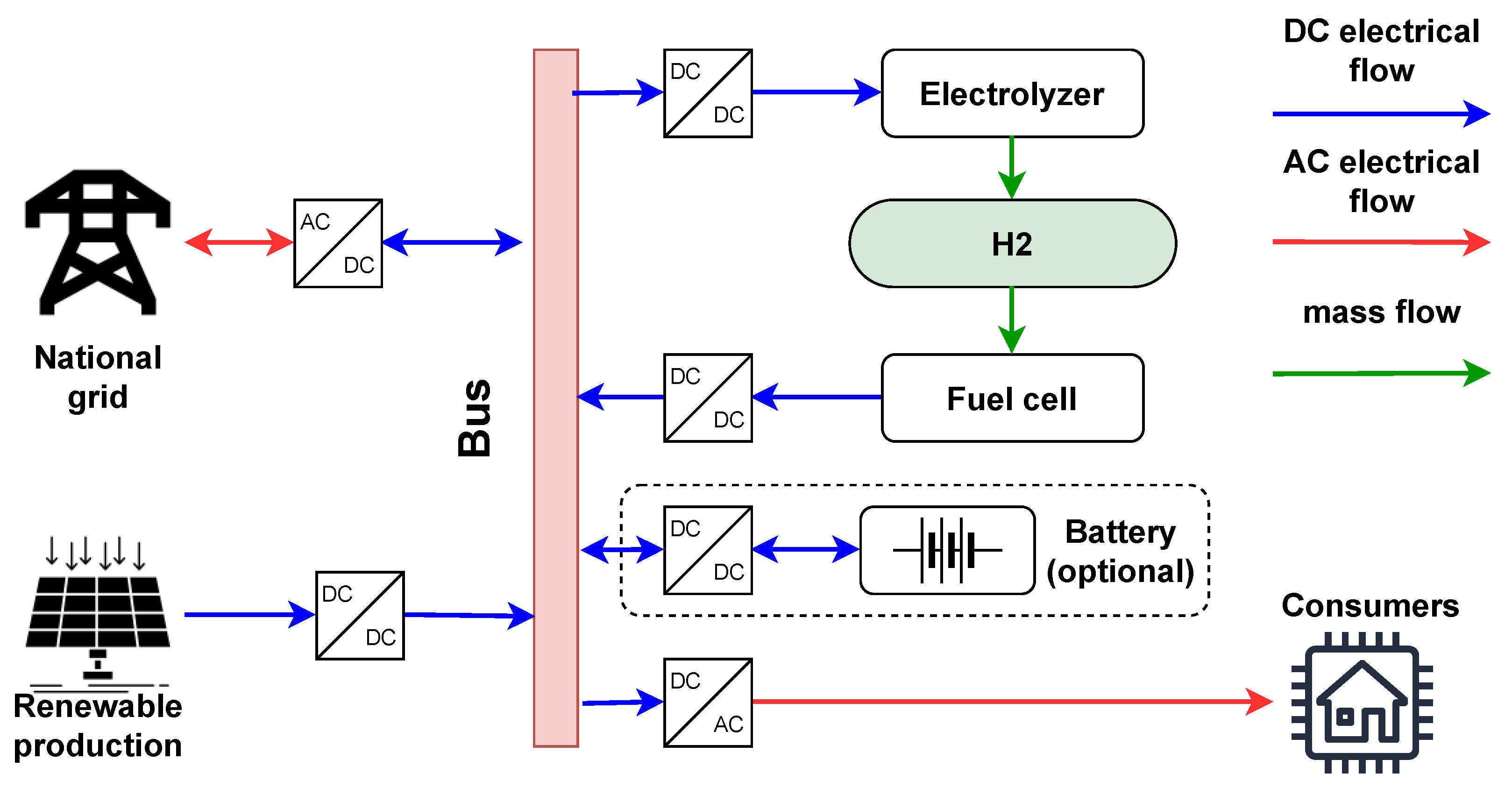
The case investigated here is a microgrid composed of one house equipped with PV panels, a battery and a P2P H${}_2$ system, illustrated in Figure 2. With the house being connected to the electrical grid, the objective of the system is to reduce its dependency to the grid and its expenses.

3.2. Optimization Settings

The objective of the optimization is to size the different equipment. The scipy-optimize python library [65] was used to perform optimization. First, a Bayesian method is used to locate the global minimum neighborhood. Then, a simplex algorithm (Nelder–Mead method) is applied to refine the results.

This case being applied to one house, restrictions on the size of equipment are implemented because of volume considerations. The chosen boundaries are presented in

Table 3. Optimization values with their bounds.

Name	Bounds
Battery	0.5 kWh	20 kWh
Electrolyzer	1 kW	10 kW
Fuel cell	1 kW	10 kW
Fuel tank	0.1 kg	20 kg
PV panels	1 kW	17 kW

: they are of the same order of magnitude as the load. PV panel’s max size is determined by the house size (see Equation (2)). The fuel tank size is based on geometric considerations: taking a pressure of 100 bar and a temperature of 55 ${}^{\circ }\mathrm{C}$ and a maximum mass of 20 kg, ending with a volume around 2.5 m${}^3$, which is already quite big.

The optimization target takes into account both independence from the grid and economic performance.

The independence criterion, ${ϵ}_{Ind}$, is equal to the total of all exchanges made with the grid (both the energy bought, $E_b$, and the energy sold, $E_s$) divided by the energy bought when none of the considered equipment (3) is present, $E_b^{ref}$ (7a). Thus, this criterion is equal to 1 when no equipment is present and, as energy sold to the grid is accounted for negatively, it penalizes solutions relying on a blatant oversizing of the PV panels.

The criterion measuring economic performance, ${ϵ}_{Eco}$, is calculated by summing all the money flows: $M_e$ for the money earned from the grid, $M_s$ for the money given to the grid, the OPEX and the CAPEX. This sum is divided by the money spent when there is no equipment, $M_s^{ref}$ (7b).

As these two criteria are normalized, the final criterion, ${ϵ}_{Tot}$, is the sum of the precedent criteria (7c):

$$\begin{array}{c}\hfill {ϵ}_{Ind}=\frac{E_b+E_s}{E_b^{ref}}\end{array}$$

(7a)

$$\begin{array}{c}\hfill {ϵ}_{Eco}=\frac{F_e-F_s+\mathrm{OPEX}+\mathrm{CAPEX}+F_s^{ref}}{F_s^{ref}}\end{array}$$

(7b)

$$\begin{array}{c}\hfill {ϵ}_{Tot}={ϵ}_{Ind}-{ϵ}_{Eco}\end{array}$$

(7c)

3.3. Strategy

The aim of this strategy is to limit the exchanges with the grid. Consequently, it always uses all the storage power available to either satisfy consumption or absorb production in excess. As detailed in Algorithm 1, the battery is employed in priority: it is faster to start than the hydrogen system but loses energy over time.

Algorithm 1 Algorithm of the first case strategy

$\mathsf{\Delta }E\leftarrow Cons.-Prod.$

if $\mathsf{\Delta }E>0$ then

$\mathsf{\Delta }E\leftarrow max(\mathsf{\Delta }E-P_{out}^{bat}·\mathsf{\Delta }t,0)$

if $\mathsf{\Delta }P>0$ then

$\mathsf{\Delta }E\leftarrow max(\mathsf{\Delta }E-P_{out}^{{\mathrm{H}}_2}·\mathsf{\Delta }t,0)$

end if

else if $\mathsf{\Delta }E<0$ then

$\mathsf{\Delta }E\leftarrow min(\mathsf{\Delta }E+P_{in}^{bat}·\mathsf{\Delta }t,0)$

if $\mathsf{\Delta }E<0$ then

$\mathsf{\Delta }E\leftarrow min(\mathsf{\Delta }E+P_{in}^{{\mathrm{H}}_2}·\mathsf{\Delta }t,0)$

end if

end if

$E^{exchanges}\leftarrow \mathsf{\Delta }E$

3.4. Simulation Plan

Several independent runs are realized to understand better how the optimization behaves. A central case is realized using exactly the elements described above, but some variations are tested around this case:

• Economic only: the self-sufficiency criterion is not considered here. This configuration and the following one help to identify the impact of each criterion on the final sizing, which relies on a mixed criterion;
• Self-sufficiency only: the economic criterion is not considered here;
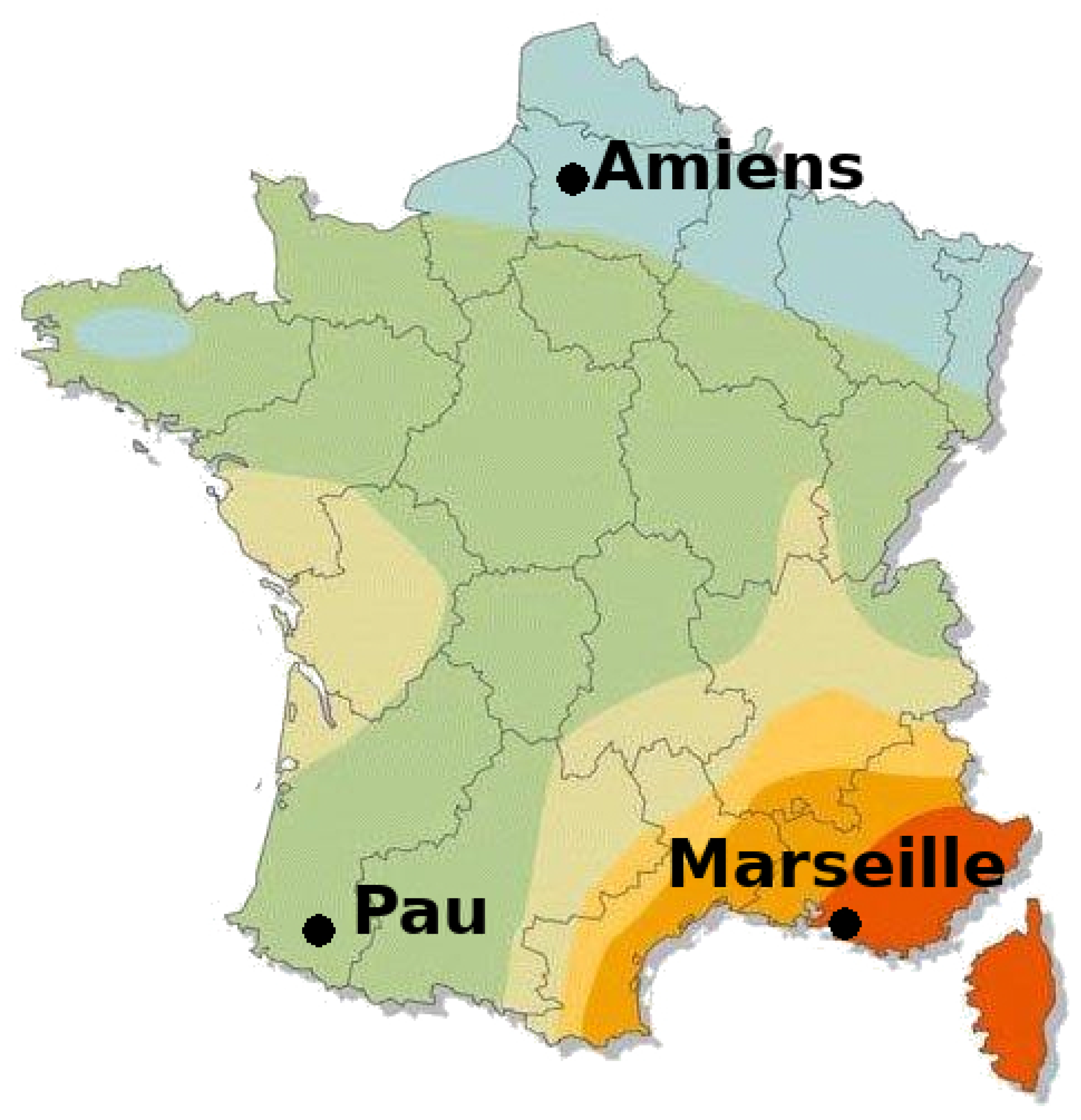
• Sunnier climate: the meteorological data taken correspond to the city of Marseille, a sunnier French city (+25% irradiation). This configuration, like the next one, tests the robustness of the results obtained for the different regions of mainland France in terms of solar resource, as illustrated in Figure 3;
• Cloudier climate: the meteorological data taken correspond to the city of Amiens, a cloudier French city (−17.5% irradiation);
• Pricesx2: prices are multiplied by 2, for both buying and selling. This configuration reduces the importance of the CAPEX;
• Equal prices: prices are the same for buying and selling energy. This configuration makes it more economically interesting to sell energy excess to the grid.

3.5. Results

Results and Discussion

The sizing obtained after the optimization can be seen in

Table 4. Result of the sizing.

Run	Sizing
	PV Panels (kW)	Battery (kWh)	Electrolyzer (kW)	Fuel Cell (kW)	Fuel Tank (kg)
Central case	12.3	7.0	4.6	1.3	1.4
Economic only	6.8	0.5 ${}^1$	1.0 ${}^1$	1.0 ${}^1$	0.2
Self-sufficiency only	16.1	11.9	10.0 ${}^2$	8.2	20 ${}^2$
Sunnier climate	10.3	4.1	5.0	2.2	1.4
Cloudier climate	11.8	2.5	4.1	1.2	0.9
Pricesx2	16.2	11.6	7.0	2.2	3.4
Equal prices	13.4	9.3	3.2	1.2	0.9

¹ minimum allowed, ² maximum allowed.

. As it can be observed, the H${}_2$ P2P system is really developed in only 2 cases over 7: in Self-sufficiency only and in Pricesx2. In the other runs, the fuel tank does not go beyond 1.4 kg of H${}_2$ stored, while the sizings of the electrolyzer and the fuel cell remain small. Meanwhile, it is observed that the electrolyzer is always bigger than the fuel cell (two times more on average). It means that the P2P system is faster to charge than to discharge. It comes from the nature of the production and the load. The former is concentrated around midday, so the peak power of the electrolyzer is important. The latter, meanwhile, is more spread over the evening and the night: as the energy available is low compared to consumption all over the night, stored energy can be delivered slowly. Thus, there is no need for a high power for discharge, i.e., an important fuel cell.

The battery is more popular, as it is encountered in all configurations, but Economic only. In Central case, 7 kWh are installed. This capacity increases, unsurprisingly, for Self-sufficiency only (11.9 kWh), where the cost does not count, and also in Pricesx2 (11.6 kWh) and Equal prices (9.3 kWh), where the investment costs are less critical. On the contrary, batteries are smaller in Sunnier climate (4.1 kWh) and Cloudier climate (2.5 kWh), for different reasons. In the first case, PV production is more spread along the day, fitting better with consumption. Consequently, less storage is needed. On the contrary, in the second case, less efficient energy production leads to a global reduction of installed capacities to save money.

Concerning PV panels, they are installed in every configuration, but the upper limit (17 kW) is never reached. In addition, 12.3 kw are installed in Central case. Like for batteries, and for the same reasons, more PV is used in Self-sufficiency only (16.1 kW), Pricesx2 (16.2 kW) and Equal prices (13.4 kW). It is stable in Cloudier climate (11.8 kW) because they are less cost-efficient (but there is a bad impact on performance).

Table 5. Final performance in case 1.

Run	Self-Sufficiency			Economy
	Bought (kWh/kWh)	Sold (kWh/kWh)	Total	Money Flow (€/€)	CAPEX (€/€)	Total
Central case	0.44	0.03	0.47	0.66	0.50	1.16
Economic only	0.67	0.05	0.72	0.77	0.23	0.99
Self-sufficiency only	0.29	0.03	0.32	0.68	0.95	1.63
Sunnier climate	0.42	0.02	0.44	0.63	0.44	1.07
Cloudier climate	0.56	0.02	0.58	0.76	0.42	1.18
Pricesx2	0.31	0.09	0.40	0.46	0.36	0.82
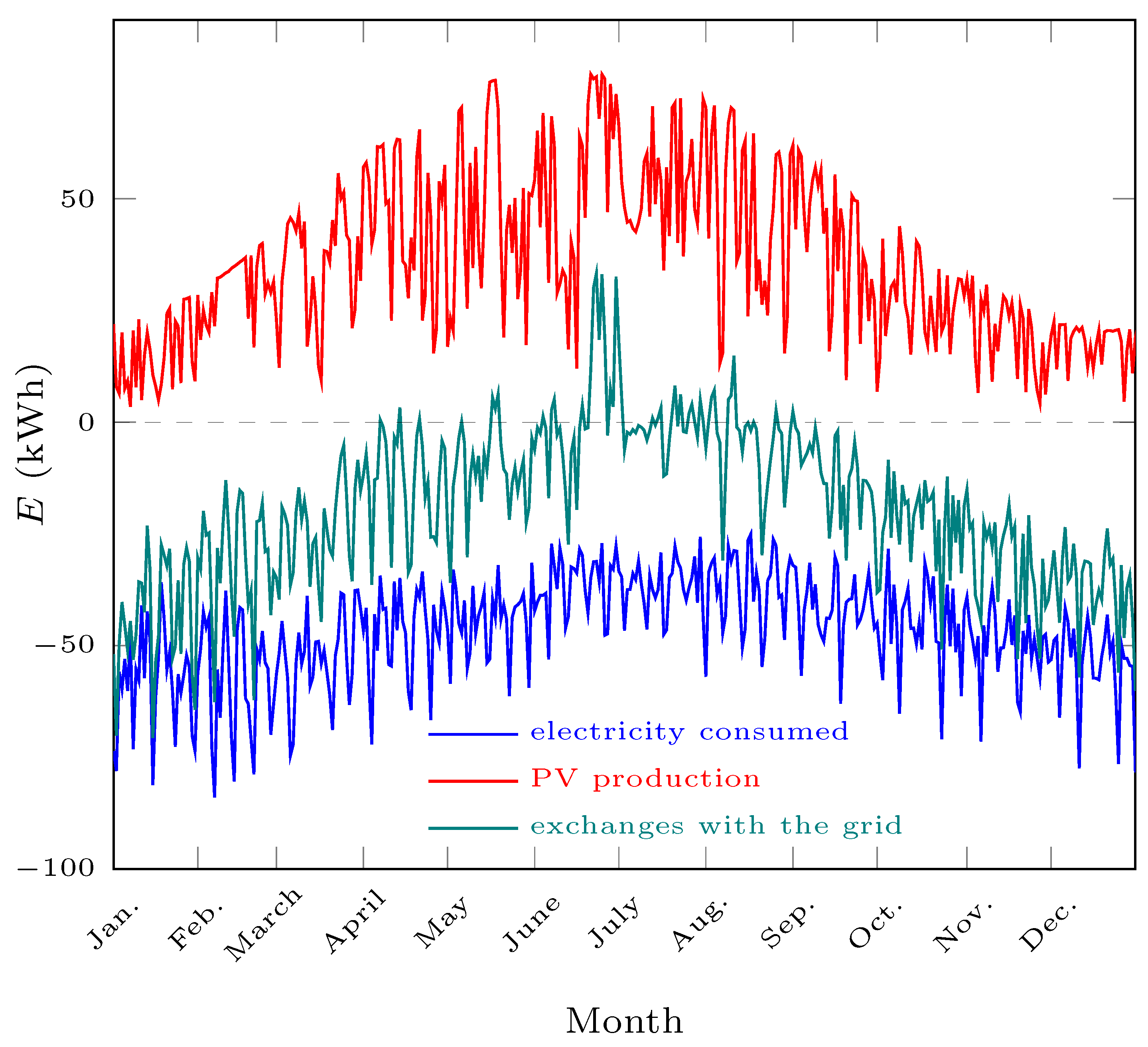
Equal prices	0.41	0.09	0.50	0.58	0.53	1.11

gives the performance of the different sizings in relative values. Self-sufficiency is compared to the total consumption of the dwelling. Economic balances are compared to the expenses made by the dwelling without any equipment: 0 means that no money is spent and 1 that no money is saved or lost. Above 1, the consumer is losing money. Overall, a very small quantity of energy is sold to the grid (5% on average), as it can be seen in Figure 4, illustrating the central case. The prosumer is also almost always losing money: this is not surprising as no subsidies were considered and as intraday prices are generally lower than regulated ones, reducing the possibility to save money.

First, the results of Economic only and Self-sufficiency only runs reveal that Central case cannot go below 30% of energy bought and sold to the grid, and that it cannot save money. In the Central case configuration, energy bought to the grid is divided by 2, but at the cost of a 16% increase of expenses for prosumers.

Concerning the climate effect, Sunnier climate is unsurprisingly the most efficient in the solar-based energy production set-up (but note that, in the cloudier region, renewable production is more focused on wind turbines). It can be seen that irradiation variation of about 20 more or less lead to smaller variations in terms of performance, 44 and 58% of energy is exchanged with the grid (−6% and +23% compared to the Central case) and the increase in expenses is equal to 7 and 18% (−8% and +2%). Thus, performances of the whole system are quite robust, at least for mainland France.

The best configuration is Pricesx2, thanks to its economic performance, which is the best of the seven runs. Equal prices is not really different from Central case: as expected, it sells more PV production to the grid than most other cases (9% of the total consumption), but this does not lead to a big improvement in the economic performance (1.11 compared to 1.16 in Central case).

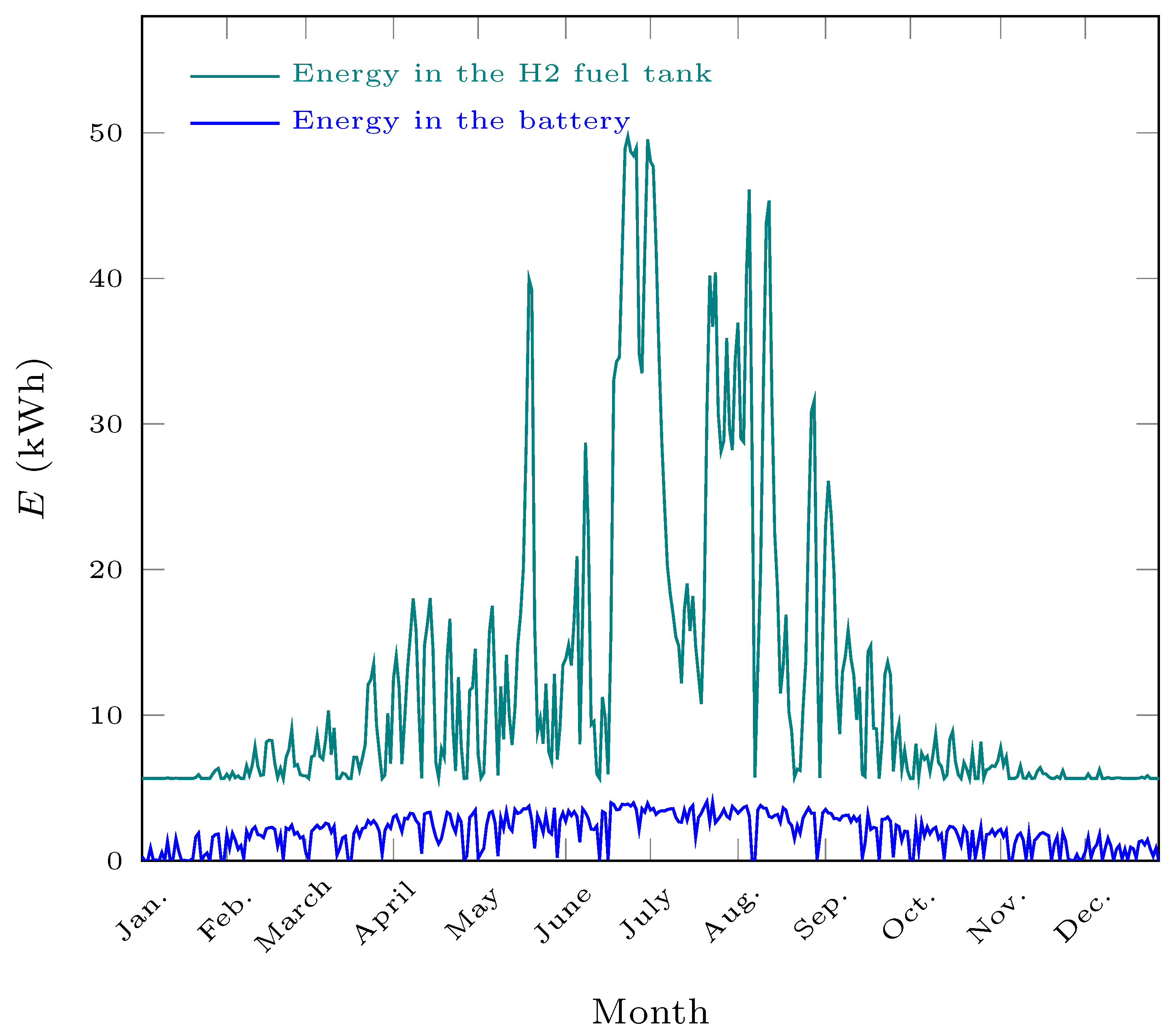
Overall, some observations can be made. In a connected grid, storage is still too costly to be economically efficient without any incentives: it appears only when exchanges with the grid are penalized. In addition, even in this case, the battery is favored, as it is cheaper than a H${}_2$ P2P system. Meanwhile, H${}_2$ P2P has an interest from a self-sufficiency point of view, as it is deployed in Self-sufficiency only or when CAPEX is less critical, like in Pricesx2: there is almost no energy degradation over the time. This is observable in Figure 5, where it is clear that the P2P system follows a yearly cycle, while batteries’ cycles are much shorter. Furthermore, the low prices values leading to small equipment sizes for storage in general and H${}_2$ in particular are taken from the past and the electricity price has risen drastically during the last six months (+35% over 2021, according to a communiqué from the French government [66]).

4. Second Case Study: Collective Bus Recharge

4.1. Case Description

This second case was elaborated after the first one, where H${}_2$ seems unsuitable for a connected microgrid in a P2P perspective. As islanded microgrids are not really relevant in our context (mainland France), a microgrid having a specific usage for H${}_2$ is chosen. If H${}_2$-fueled cars are still rare in France, a fleet of buses propelled by H${}_2$ is currently being exploited in the agglomeration of Pau, the place corresponding to the meteorological data. Thus, the second study bears on the production of green H${}_2$ destined to a local consumption, the refueling of H${}_2$ buses.

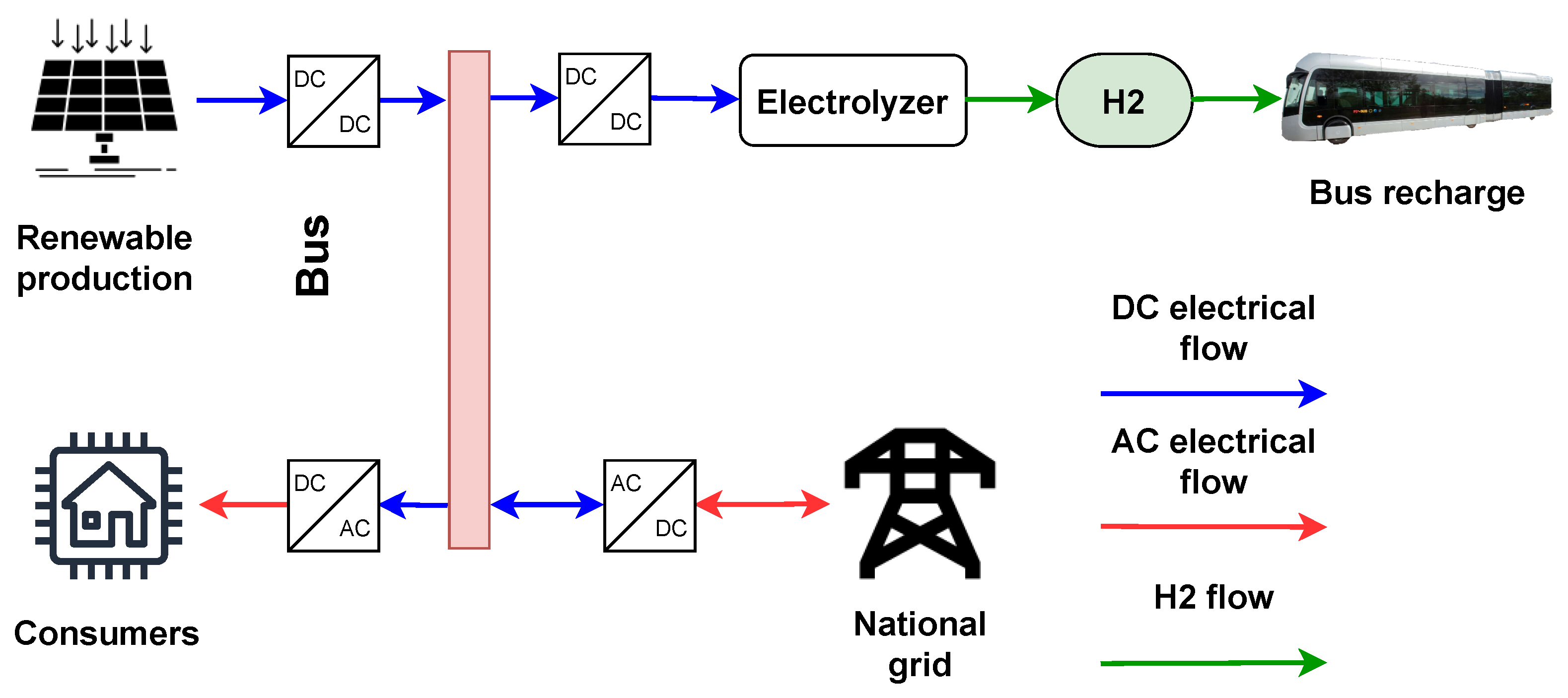
The investigated microgrid is composed of several houses equipped with PV panels. The goal here is to identify the size of a system able to refuel a bus on a daily basis and to assess H${}_2$ production cost (if any). According to to IAE and IRENA estimations, H2 produced via renewable energy ranges from 3 to 8 $/kg [67] and 2.7 to 7 $/kg [68], respectively. For further comparison, a study was conducted for a refuelling ${\mathrm{H}}_2$ station in Halle, Belgium and found a cost of 10.3 €/ kg [69]. This system is composed of houses equipped with individual PV panels, a collective electrolyzer, and a collective fuel tank, as illustrated in Figure 6.

4.2. Optimization Settings

The objective of the optimization is still to size the different equipment. The method is the same as before: a two-phase optimization process is used, with a Bayesian first and then a simplex in second. The quantity of photovoltaic production is represented by the number of houses, as it is considered that each house is equipped with the maximum of PV panels, 17 kW (see Equation (2)). This approach was used to avoid discontinuities in the evaluation function: otherwise, adding 1 W of PV can lead to adding a supplementary load of one full house.

The optimization target takes into account the economic performance, trying to minimize the number of houses and penalizes the non-delivery of H${}_2$. The criterion measuring economic performance is the same as the one used in the first case (7b).

The “number of houses” criterion ${ϵ}_{houses}$ is simply defined as the number of houses, $N_{houses}$, multiplied by a weighing coefficient, $C_{houses}$, taken equal to 0.001: this setting makes values comparable to the economic criterion, avoiding it from being either dominant or ignored (8a).

The penalty for a lack of H${}_2$ in the tank, ${ϵ}_{service}$, is the proportion of energy lacking, $E_{lacking}$ compared to the energy needed for one delivery, $E_{daily}$, multiplied by a weighing coefficient $C_{service}$, taken equal to 0.5, a value large enough to ensure the optimization avoids non-delivery at all cost. Nonetheless, it must not be too high; otherwise, it will hamper the optimizer.

The final criterion, ${ϵ}_{Tot}$, is the sum of the three criteria (8c):

$$\begin{array}{c}\hfill {ϵ}_{houses}=N_{houses}·C_{houses}\end{array}$$

(8a)

$$\begin{array}{c}\hfill {ϵ}_{service}=\frac{E_{lacking}}{E_{daily}}·C_{service}\end{array}$$

(8b)

$$\begin{array}{c}\hfill {ϵ}_{Tot}={ϵ}_{houses}+{ϵ}_{service}-{ϵ}_{Eco}\end{array}$$

(8c)

4.3. Strategy

The objective in this case study is to use excess PV production to produce green H${}_2$. Nonetheless, the priority is still to satisfy the consumption of the users with renewable energy. Thus, the production is first affected by self-consumption and second to the recharge of the bus. In one configuration, the use of a battery is considered: there, it comes in third position. Finally, the potential remaining energy is sold to the grid (Algorithm 2).

Algorithm 2 Algorithm of the second case strategy

$\mathsf{\Delta }E\leftarrow E_{Cons.}-E_{Prod.}$

if $\mathsf{\Delta }E>0$ then

$\mathsf{\Delta }E\leftarrow max(\mathsf{\Delta }E-P_{out}^{bat}·\mathsf{\Delta }t,0)$

else if $\mathsf{\Delta }E<0$ then

$\mathsf{\Delta }E\leftarrow min(\mathsf{\Delta }E+P_{in}^{{\mathrm{H}}_2}·\mathsf{\Delta }t,0)$

if $\mathsf{\Delta }E<0$ then

$\mathsf{\Delta }E\leftarrow min(\mathsf{\Delta }E+P_{in}^{bat}·\mathsf{\Delta }t,0)$

end if

end if

$P^{exchanges}\leftarrow \mathsf{\Delta }E$

4.4. Simulation Plan

Like in the first case study, some variations around the central configuration were assessed. Most of them are similar to the previous variations, but three of them need a complementary explanation:

• half-covered house: in this configuration, houses are only authorized to install half of their max PV capacity: it can be expected to lead to an increase in the number of houses, and thus to increase self-consumption of PV and reduce the investment cost proportion, ultimately leading to cheaper H${}_2$;
• Battery: a battery is added, stemming from the observation that a non-negligible amount of PV is sold to the grid in the central case;
• Minimum houses: the economic performance is not taken into account;
• Sunnier climate;
• Cloudier climate;
• Pricesx2;
• Equal prices.

An optimization not seeking to limit the number of houses involved was tried, but it was not conclusive: as the economic performance becomes the only criterion, it tends to include an unlimited number of houses in order to minimize the individual cost of collective equipment.

4.5. Results and Discussion

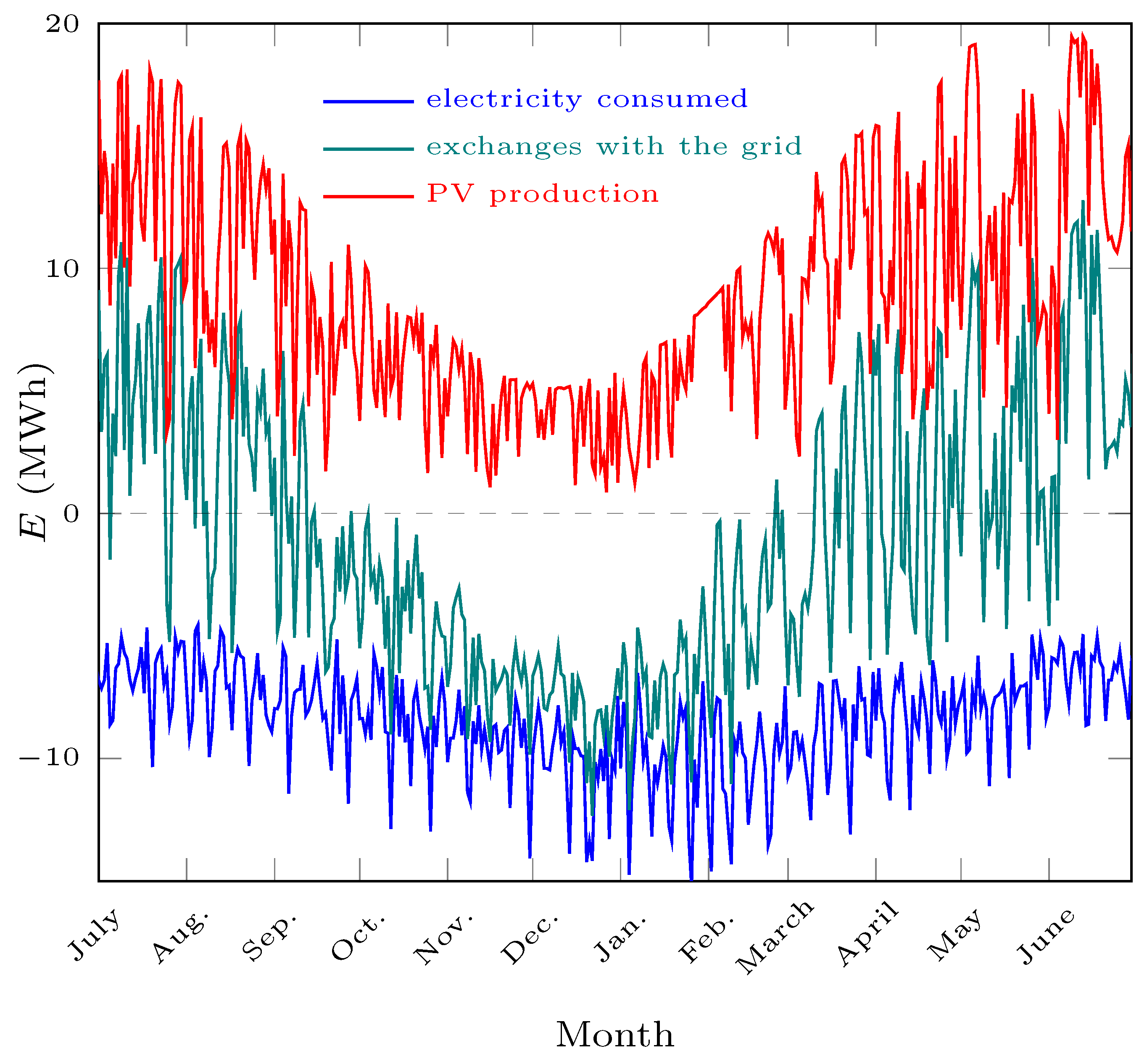
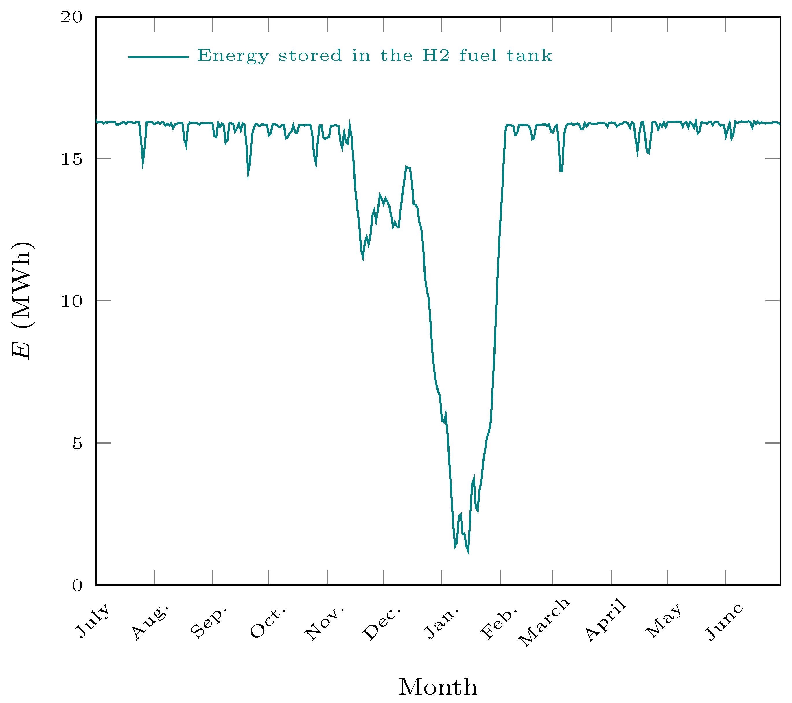
The sizing results of this second case are available in

Table 6. Results of the optimization.

Run	Sizing
	Number of Houses	Battery (kWh)	Electrolyzer (kW)	Fuel Tank (kg)
Central case	182	NA	622	434
Half-covered house	267	NA	540	2882
Battery	180	1.2	528	499
Minimum houses	56	NA	800	9152
Sunnier climate	148	NA	455	144
Cloudier climate	221	NA	530	2010
Pricesx2	149	NA	478	739
Equal prices	222	NA	485	394

, and the related performance are given in

Table 7. Final performance in case 2.

Run	Number of Houses	Economy			Non-Service	H${}_2$ Cost (€/kg)
		Money Flow (€/€)	CAPEX (€/€)	Total
Central case	182	0.68	0.51	1.19	0	5.24
Half-covered house	267	0.80	0.23	1.13	0	5.20
Battery	180	0.68	0.51	1.19	0	5.49
Minimum houses	56	1.29	1.64	2.93	0	31.38
Sunnier climate	148	0.59	0.50	1.09	0	0.26
Cloudier climate	221	0.76	0.56	1.32	0	14.49
Pricesx2	149	0.61	0.27	0.88	0	−15.15
Equal prices	222	0.38	0.50	0.88	0	−13.22

. In Figure 7 and Figure 8, the yearly PV production, electricity consumption, net exchanges with the grid and the amount of energy stored in the fuel tank in the base configuration are displayed. Comparing the two figures, it can be seen that rebound in the fuel tank, from November–December, is caused by an increase in the mean PV production due to nice weather during the same period. The fuel tank never reaches 0 because of pressure constraints.

In all scenarios, it is possible to meet the consumption of one bus-tank of hydrogen with fewer than 300 houses for all configurations and a minimum of 56, at a cost of (+138%).

As predicted, the covering of only half the available surface by photovoltaic panels while maintaining the required H${}_2$ output leads to an increase in the number of necessary houses to meet the demand (+47%). While the increase of self-consumption comes with an increase of the energy purchased from the grid, the better usage of the H${}_2$ system reduces the total cost and thus leads to cheaper H${}_2$.

Since the criterion does not have an independence component, and is mostly economic, it is not surprising that, even though it is observed that a significant surplus of PV power is to be sold to the grid (+41% by averaging to one dwelling), the optimisation process does not select a battery of notable size.

In a sunnier climate, fewer houses (−18%) and a relative smaller fuel tank (−67%) are needed in comparison to a cloudier climate which requires a huge fuel tank (+363%), as carrying the excessive energy from the summer into the winter.

As in the first case, the increase of the energy prices and the omission of the transportation cost are favorable to hydrogen. The negative values of H${}_2$ cost for those two configurations means that the gains from the photo-voltaic production and auto-consumption are sufficient to cover the cost of the hydrogen production.

The H${}_2$ cost is the price H${}_2$ should have to reach a level of expense equal to the one without any equipment. Thus, the real price should be higher (or there should be incentives) for the system to be profitable to prosumers.

5. Conclusions

In this paper, an architecture able to model various grid configurations and management strategies was presented. It was applied to two cases: a single dwelling concerned about its energy expenses, and a solar community that has to generate enough hydrogen to refuel a bus on a daily basis. In both cases, the study took place in the French context, i.e., prices, meteorological data, and consumption profile correspond to French data.

In the first case, the pertinence of using storage to improve the self-consumption and the money savings at a domestic scale is assessed. Equipment sizing was made using two criteria: independence from the grid and economic performance. There, energy storage solutions relying on H${}_2$ are interesting only if the economic performance is neglected (Self-sufficiency configuration) in the evaluation process or if the prices of energy are slightly higher (Pricesx2 configuration). The impact of climate (mainly the irradiation here, as the production is solar-based) seems mitigated by storage technologies. Overall, storage is still too costly to be economically efficient and the long-term advantage of H${}_2$ in terms of energy loss does not compensate the lower cost of the battery. It is interesting to note that, with the prices taken, i.e., real intraday prices, even the PV alone is not profitable. This highlights the importance of incentives/subsidies to support the development of renewable energy production and storage.

In the second case, the non-consumed part of PV production was used to produce H${}_2$ directly for a local usage: here, the refueling of a bus, with a collective fuel cell and fuel tank, at the scale of a community. The idea was to find a better usage for the excess PV production than selling it to the grid. Beyond the sizing of the electrolyzer and the fuel tank, the relations between number of houses and the cost price of H${}_2$ (defined at the cost at which prosumers expense with the equipment are equal to the ones without any equipment) were analyzed. In the studied context, less than 100 houses can be sufficient, but for a high H${}_2$ cost (31.38 €/kg for 56 houses). The relative importance of the cost of the electrolyzer and the fuel tank in the global economic performance tend to decrease with the number of houses (as there are more people paying for equipment of a similar size). Consequently, the more houses, the cheaper the H${}_2$. The compromise reached in central case is of 5.26 €/kg for 182 houses. This price is also in the range of IEA estimations (3–8 $/kg). Thus, this second low-scale usage of H${}_2$ seems much more promising to us than the first, especially knowing that H${}_2$ is promoted by the French government.

Overall, this study, made in a French context and considering no financial incentives, tends to show the following results:

• In the first case, H${}_2$, used as a mean of storing electricity, is not economically competitive compared to batteries;
• Use of non self-consumed solar energy to produce collectively H${}_2$ allows for reaching an H${}_2$ price comparable to the ones found in literature. It seems a promising way to produce locally green hydrogen while bringing benefits to consumers.

Furthermore, it is expected that the price of energy will continue to rise, with new controllable systems (like H${}_2$ systems) and prosumers and demand response programs appearing and diffusing, increasing slightly the complexity of energy management. In this context, basic supervision strategies could be insufficient: several studies [70], reveal that Artificial Intelligence techniques are quite efficient at handling such complexity.

References

- Energy Storage Grand Challenge Energy Storage Market Report. Technical Report NREL/TP-5400-78462 DOE/GO-102020-5497. 2020; p. 65. Available online: https://www.energy.gov/sites/default/files/2020/12/f81/Energy%20Storage%20Market%20Report%202020_0.pdf (accessed on 11 May 2022).
- Spitsen, P. Energy Storage Grand Challenge Roadmap. 2020; p. 157. Available online: https://www.energy.gov/energy-storage-grand-challenge/articles/energy-storage-grand-challenge-roadmap (accessed on 11 May 2022).
- Joint EASE/EERA Recommendations for a European Energy Storage Technology Development Roadmap. 2017. Available online: https://www.eera-set.eu/component/attachments/?task=download&id=312 (accessed on 11 May 2022).
- Technology Roadmap Energy Storage. International Energy Agency. 2014, p. 64. Available online: https://iea.blob.core.windows.net/assets/80b629ee-597b-4f79-a236-3b9a36aedbe7/TechnologyRoadmapEnergystorage.pdf (accessed on 11 May 2022).
- Tan, K.M.; Babu, T.S.; Ramachandaramurthy, V.K.; Kasinathan, P.; Solanki, S.G.; Raveendran, S.K. Empowering Smart Grid: A Comprehensive Review of Energy Storage Technology and Application with Renewable Energy Integration. J. Energy Storage 2021, 39, 102591. [Google Scholar] [CrossRef]
- Zhang, F.; Zhao, P.; Niu, M.; Maddy, J. The Survey of Key Technologies in Hydrogen Energy Storage. Int. J. Hydrog. Energy 2016, 41, 14535–14552. [Google Scholar] [CrossRef]
- Elliott, D. Energy Storage Systems; (Book Chapter); IOP Publishing: Bristol, UK, 2017. [Google Scholar]
- DeValeria, M.K.; Michaelides, E.E.; Michaelides, D.N. Energy and Thermal Storage in Clusters of Grid-Independent Buildings. Energy 2020, 190, 116440. [Google Scholar] [CrossRef]
- Vand, B.; Ruusu, R.; Hasan, A.; Manrique Delgado, B. Optimal Management of Energy Sharing in a Community of Buildings Using a Model Predictive Control. Energy Convers. Manag. 2021, 239, 114178. [Google Scholar] [CrossRef]
- Medved, S.; Domjan, S.; Arkar, C. Contribution of Energy Storage to the Transition from Net Zero to Zero Energy Buildings. Energy Build. 2021, 236, 110751. [Google Scholar] [CrossRef]
- Romanchenko, D.; Nyholm, E.; Odenberger, M.; Johnsson, F. Impacts of Demand Response from Buildings and Centralized Thermal Energy Storage on District Heating Systems. Sustain. Cities Soc. 2021, 64, 102510. [Google Scholar] [CrossRef]
- Touretzky, C.R.; Baldea, M. A Hierarchical Scheduling and Control Strategy for Thermal Energy Storage Systems. Energy Build. 2016, 110, 94–107. [Google Scholar] [CrossRef]
- Ibrahim, H.; Ilinca, A.; Perron, J. Energy Storage Systems—Characteristics and Comparisons. Renew. Sustain. Energy Rev. 2008, 12, 1221–1250. [Google Scholar] [CrossRef]
- Khouya, A. Levelized costs of energy and hydrogen of wind farms and concentrated photovoltaic thermal systems. A case study in Morocco. Int. J. Hydrog. Energy 2020, 45, 31632–31650. [Google Scholar] [CrossRef]
- Khouya, A. Hydrogen production costs of a polymer electrolyte membrane electrolysis powered by a renewable hybrid system. Int. J. Hydrog. Energy 2021, 46, 14005–14023. [Google Scholar] [CrossRef]
- Van der Roest, E.; Snip, L.; Fens, T.; van Wijk, A. Introducing Power-to-H3: Combining renewable electricity with heat, water and hydrogen production and storage in a neighbourhood. Appl. Energy 2020, 257, 114024. [Google Scholar] [CrossRef]
- Muthiah-Nakarajan, V.; Cherukuri, S.H.C.; Saravanan, B.; Palanisamy, K. Residential Energy Management Strategy Considering the Usage of Storage Facilities and Electric Vehicles. Sustain. Energy Technol. Assess. 2021, 45, 101167. [Google Scholar] [CrossRef]
- Bernal-Agustín, J.L.; Dufo-López, R. Simulation and Optimization of Stand-Alone Hybrid Renewable Energy Systems. Renew. Sustain. Energy Rev. 2009, 13, 2111–2118. [Google Scholar] [CrossRef]
- Okedu, K.E.; Uhunmwangho, R. Optimization of Renewable Energy Efficiency Using HOMER. Int. J. Renew. Energy Res. 2014, 4, 8. [Google Scholar]
- Masud, A.A. The Application of Homer Optimization Software to Investigate the Prospects of Hybrid Renewable Energy System in Rural Communities of Sokoto in Nigeria. Int. J. Electr. Comput. Eng. (IJECE) 2017, 7, 596. [Google Scholar] [CrossRef] [Green Version]
- Khare, V.; Nema, S.; Baredar, P. Optimization of Hydrogen Based Hybrid Renewable Energy System Using HOMER, BB-BC and GAMBIT. Int. J. Hydrog. Energy 2016, 41, 16743–16751. [Google Scholar] [CrossRef]
- Alsharif, M.H. Optimization Design and Economic Analysis of Energy Management Strategy Based on Photovoltaic/Energy Storage for Heterogeneous Cellular Networks Using the HOMER Model. Sol. Energy 2017, 147, 133–150. [Google Scholar] [CrossRef]
- Kumar, P.; Pukale, R.; Kumabhar, N.; Patil, U. Optimal Design Configuration Using HOMER. Procedia Technol. 2016, 24, 499–504. [Google Scholar] [CrossRef]
- Gökçek, M.; Kale, C. Techno-Economical Evaluation of a Hydrogen Refuelling Station Powered by Wind-PV Hybrid Power System: A Case Study for İzmir-Çeşme. Int. J. Hydrog. Energy 2018, 43, 10615–10625. [Google Scholar] [CrossRef]
- Balachander, K.; Suresh Kumaar, G.; Mathankumar, M.; Manjunathan, A.; Chinnapparaj, S. Optimization in Design of Hybrid Electric Power Network Using HOMER. Mater. Today Proc. 2021, 45, 1563–1567. [Google Scholar] [CrossRef]
- Khalil, L.; Liaquat Bhatti, K.; Arslan Iqbal Awan, M.; Riaz, M.; Khalil, K.; Alwaz, N. Optimization and Designing of Hybrid Power System Using HOMER Pro. Mater. Today Proc. 2021, 47, S110–S115. [Google Scholar] [CrossRef]
- Ekren, O.; Hakan Canbaz, C.; Güvel, Ç.B. Sizing of a Solar-Wind Hybrid Electric Vehicle Charging Station by Using HOMER Software. J. Clean. Prod. 2021, 279, 123615. [Google Scholar] [CrossRef]
- Singh, A.; Baredar, P.; Gupta, B. Computational Simulation & Optimization of a Solar, Fuel Cell and Biomass Hybrid Energy System Using HOMER Pro Software. Procedia Eng. 2015, 127, 743–750. [Google Scholar] [CrossRef] [Green Version]
- Zakeri, B.; Cross, S.; Dodds, P.; Gissey, G.C. Policy Options for Enhancing Economic Profitability of Residential Solar Photovoltaic with Battery Energy Storage. Appl. Energy 2021, 290, 116697. [Google Scholar] [CrossRef]
- Stadler, M.; Cardoso, G.; Mashayekh, S.; Forget, T.; DeForest, N.; Agarwal, A.; Schönbein, A. Value Streams in Microgrids: A Literature Review. Appl. Energy 2016, 162, 980–989. [Google Scholar] [CrossRef] [Green Version]
- Sreedhar, I.; Kamani, K.M.; Kamani, B.M.; Reddy, B.M.; Venugopal, A. A Bird’s Eye View on Process and Engineering Aspects of Hydrogen Storage. Renew. Sustain. Energy Rev. 2018, 91, 838–860. [Google Scholar] [CrossRef]
- Marocco, P.; Ferrero, D.; Gandiglio, M.; Ortiz, M.M.; Sundseth, K.; Lanzini, A.; Santarelli, M. A study of the techno-economic feasibility of H2-based energy storage systems in remote areas. Energy Convers. Manag. 2020, 211, 112768. [Google Scholar] [CrossRef]
- Marocco, P.; Ferrero, D.; Lanzini, A.; Santarelli, M. The role of hydrogen in the optimal design of off-grid hybrid renewable energy systems. J. Energy Storage 2022, 46, 103893. [Google Scholar] [CrossRef]
- Sterner, M.; Specht, M. Power-to-Gas and Power-to-X—The History and Results of Developing a New Storage Concept. Energies 2021, 14, 6594. [Google Scholar] [CrossRef]
- Chamandoust, H.; Hashemi, A.; Bahramara, S. Energy Management of a Smart Autonomous Electrical Grid with a Hydrogen Storage System. Int. J. Hydrog. Energy 2021, 46, 17608–17626. [Google Scholar] [CrossRef]
- Avril, S.; Arnaud, G.; Florentin, A.; Vinard, M. Multi-Objective Optimization of Batteries and Hydrogen Storage Technologies for Remote Photovoltaic Systems. Energy 2010, 35, 5300–5308. [Google Scholar] [CrossRef]
- Valverde-Isorna, L.; Ali, D.; Hogg, D.; Abdel-Wahab, M. Modelling the Performance of Wind–Hydrogen Energy Systems: Case Study the Hydrogen Office in Scotland/UK. Renew. Sustain. Energy Rev. 2016, 53, 1313–1332. [Google Scholar] [CrossRef]
- Morin, D.; Stevenin, Y.; Grolleau, C.; Brault, P. Evaluation of Performance Improvement by Model Predictive Control in a Renewable Energy System with Hydrogen Storage. Int. J. Hydrog. Energy 2018, 43, 21017–21029. [Google Scholar] [CrossRef] [Green Version]
- Présentation de la Stratégie Nationale pour le Développement de l’Hydrogène Décarboné en France. 2020. Available online: https://www.economie.gouv.fr/presentation-strategie-nationale-developpement-hydrogene-decarbone-france (accessed on 11 May 2022).
- Lujano-Rojas, J.M.; Dufo-López, R.; Bernal-Agustín, J.L. Probabilistic modelling and analysis of stand-alone hybrid power systems. Energy 2013, 63, 19–27. [Google Scholar] [CrossRef]
- Durbin, D.; Malardier-Jugroot, C. Review of Hydrogen Storage Techniques for on Board Vehicle Applications. Int. J. Hydrog. Energy 2013, 38, 14595–14617. [Google Scholar] [CrossRef]
- Pukazhselvan, D.; Kumar, V.; Singh, S. High Capacity Hydrogen Storage: Basic Aspects, New Developments and Milestones. Nano Energy 2012, 1, 566–589. [Google Scholar] [CrossRef]
- Sankir, M.; Demirci Sankir, N. (Eds.) Hydrogen Storage Technologies; Advances in Hydrogen Production and Storage; John Wiley & Sons, Inc.: Hoboken, NJ, USA; Scrivener Publishing LLC: Salem, MA, USA, 2018. [Google Scholar]
- Hosseini, M.; Dincer, I.; Naterer, G.; Rosen, M. Thermodynamic Analysis of Filling Compressed Gaseous Hydrogen Storage Tanks. Int. J. Hydrog. Energy 2012, 37, 5063–5071. [Google Scholar] [CrossRef]
- Yang, J.C. A Thermodynamic Analysis of Refueling of a Hydrogen Tank. Int. J. Hydrog. Energy 2009, 34, 6712–6721. [Google Scholar] [CrossRef]
- Sakoda, N.; Shindo, K.; Motomura, K.; Shinzato, K.; Kohno, M.; Takata, Y.; Fujii, M. Burnett PVT Measurements of Hydrogen and the Development of a Virial Equation of State at Pressures up to 100 MPa. Int. J. Thermophys. 2012, 33, 381–395. [Google Scholar] [CrossRef]
- Achaibou, N.; Haddadi, M.; Malek, A. Lead Acid Batteries Simulation Including Experimental Validation. J. Power Sources 2008, 185, 1484–1491. [Google Scholar] [CrossRef]
- Schiffer, J.; Sauer, D.U.; Bindner, H.; Cronin, T.; Lundsager, P.; Kaiser, R. Model Prediction for Ranking Lead-Acid Batteries According to Expected Lifetime in Renewable Energy Systems and Autonomous Power-Supply Systems. J. Power Sources 2007, 168, 66–78. [Google Scholar] [CrossRef]
- Mohsin, M.; Picot, A.; Maussion, P. Lead-acid battery modelling in perspective of ageing: A Review. In Proceedings of the 2019 IEEE 12th International Symposium on Diagnostics for Electrical Machines, Power Electronics and Drives (SDEMPED), Toulouse, France, 14 October 2019; pp. 425–431. [Google Scholar] [CrossRef]
- Dufo-López, R.; Champier, D.; Gibout, S.; Lujano-Rojas, J.M.; Domínguez-Navarro, J.A. Optimisation of Off-Grid Hybrid Renewable Systems with Thermoelectric Generator. Energy Convers. Manag. 2019, 196, 1051–1067. [Google Scholar] [CrossRef]
- Huld, T.; Müller, R.; Gambardella, A. A new solar radiation database for estimating PV performance in Europe and Africa. Sol. Energy 2012, 86, 1803–1815. [Google Scholar] [CrossRef]
- Epex Spot—European Power Exchange. Available online: https://www.europex.org/members/epex-spot/ (accessed on 24 February 2022).
- Rapport d’Évaluation du 22 Juillet 2021 sur le Dispositif des Tarifs Rélementés de Vente d’Électricité; Technical Report; Autorité de la Concurrence; Paris, France, 2021; Available online: https://www.autoritedelaconcurrence.fr/sites/default/files/2021-09/rapport-trv.pdf (accessed on 24 February 2022).
- Dufo-López, R.; Bernal-Agustín, J.L.; Yusta-Loyo, J.M.; Domínguez-Navarro, J.A.; Ramírez-Rosado, I.J.; Lujano, J.; Aso, I. Multi-Objective Optimization Minimizing Cost and Life Cycle Emissions of Stand-Alone PV–Wind–Diesel Systems with Batteries Storage. Appl. Energy 2011, 88, 4033–4041. [Google Scholar] [CrossRef]
- ENGIE: Estimer la Consommation Electrique d’Un Appartement. Available online: https://particuliers.engie.fr/economies-energie/conseils-economies-energie/conseils-eco-gestes-au-quotidien/estimer-consommation-electrique-appartement.html (accessed on 24 February 2022).
- ENGIE: Consommation Electrique Moyenne d’Un Logement par Superficie. Available online: https://particuliers.engie.fr/electricite/conseils-electricite/conseils-tarifs-electricite/consommation-electrique-moyenne-logement-par-superficie.html (accessed on 24 February 2022).
- Projected Costs of Generating Electricity 2020 Edition. 2020. Available online: https://www.iea.org/reports/projected-costs-of-generating-electricity-2020 (accessed on 11 May 2022).
- Joris, P. State-of-the art CAPEX data for water electrolysers, and their impact on renewable hydrogen price settings. Int. J. Hydrog. Energy 2019, 44, 4406–4413. [Google Scholar] [CrossRef]
- Marocco, P.; Ferrero, D.; Lanzini, A.; Santarelli, M. Manufacturing Cost Analysis of PEM Fuel Cell Systems for 5- and 10-kW Backup Power Applications; Battelle: Columbus, OH, USA, 2016. Available online: https://www.energy.gov/sites/prod/files/2016/12/f34/fcto_cost_analysis_pem_fc_5-10kw_backup_power_0.pdf (accessed on 11 May 2022).
- Study on Early Business Cases for H2 IN Energy Storage and More Broadly Power to H2 Applications—Final Report; Technical Report, Fuel Cells and Hydrogen Joint Undertaking; Tractebel Engineering S.A.: Brussels, Belgium, 2017.
- Kuckshinrichs, W.; Ketelaer, T.; Koj, J.C. Economic Analysis of Improved Alkaline Water Electrolysis. Front. Energy Res. 2017, 5. [Google Scholar] [CrossRef] [Green Version]
- Gracia, L.; Casero, P.; Bourasseau, C.; Chabert, A. Use of Hydrogen in Off-Grid Locations, a Techno-Economic Assessment. Energies 2018, 11, 3141. [Google Scholar] [CrossRef] [Green Version]
- Debray, B.; Weinberger, B. Guide pour l’Évaluation de la Conformité et la Certification des Systèmes à Hydrogè; Technical Report; 2021; Available online: https://librairie.ademe.fr/produire-autrement/4978-guide-pour-l-evaluation-de-la-conformite-et-la-certification-des-systemes-a-hydrogene.html (accessed on 11 May 2022).
- Paudyal, B.R.; Imenes, A.G. Investigation of temperature coefficients of PV modules through field measured data. Sol. Energy 2021, 224, 425–439. [Google Scholar] [CrossRef]
- Jones, E.; Oliphant, T.; Peterson, P. SciPy: Open Source Scientific Tools for Python. 2001. Available online: https://www.researchgate.net/publication/213877848_SciPy_Open_Source_Scientific_Tools_for_Python (accessed on 11 May 2022).
- Le Gouvernement Engage des Mesures Exceptionnelles pour Protéger le Pouvoir d’Achat des Français et Préserver la Compétitivité de l’Approvisionnement Électrique des Entreprises Face à la Forte Hausse des Prix de l’Énergie; The Ministry of Ecological Transition: Paris, France, 2022. Available online: https://www.ecologie.gouv.fr/gouvernement-engage-des-mesures-exceptionnelles-proteger-pouvoir-dachat-des-francais-et-preserver (accessed on 11 May 2022).
- The Future of Hydrogen; Technical Report; International Energy Agency: Paris, France, 2019.
- Hydrogen: A Renewable Energy Perspective; Technical Report; International Renewable Energy Agency—IRENA: Masdar City, United Arab Emirates, 2019.
- Viktorsson, L.; Heinonen, J.T.; Skulason, J.B.; Unnthorsson, R. A Step towards the Hydrogen Economy—A Life Cycle Cost Analysis of A Hydrogen Refueling Station. Energies 2017, 10, 763. [Google Scholar] [CrossRef]
- Antonopoulos, I.; Robu, V.; Couraud, B.; Kirli, D.; Norbu, S.; Kiprakis, A.; Flynn, D.; Elizondo-Gonzalez, S.; Wattam, S. Artificial intelligence and machine learning approaches to energy demand-side response: A systematic review. Renew. Sustain. Energy Rev. 2020, 130, 109899. [Google Scholar] [CrossRef]
Figure 1.
Algorithm overview.
Figure 2.
First case illustration.
Figure 3.
Solar resource in France, according to ADEME.
Figure 4.
Energy flows in the first case over one year, on a daily basis, from January to December.
Figure 5.
Storage evolution in the first case over one year, on a daily basis, from January to December.
Figure 6.
Second case illustration.
Figure 7.
Energy flows in the second case over one year, on a daily basis, from June to May.
Figure 8.
Storage evolution in the second case over one year, on a daily basis, from June to May.