
An Improved Method of Clay-Induced Rock Typing Derived from Log Data in Modelling Low Salinity Water Injection: A Case Study on an Oil Field in Indonesia

 and
and
Abstract
:1. Introduction
2. Field Overview
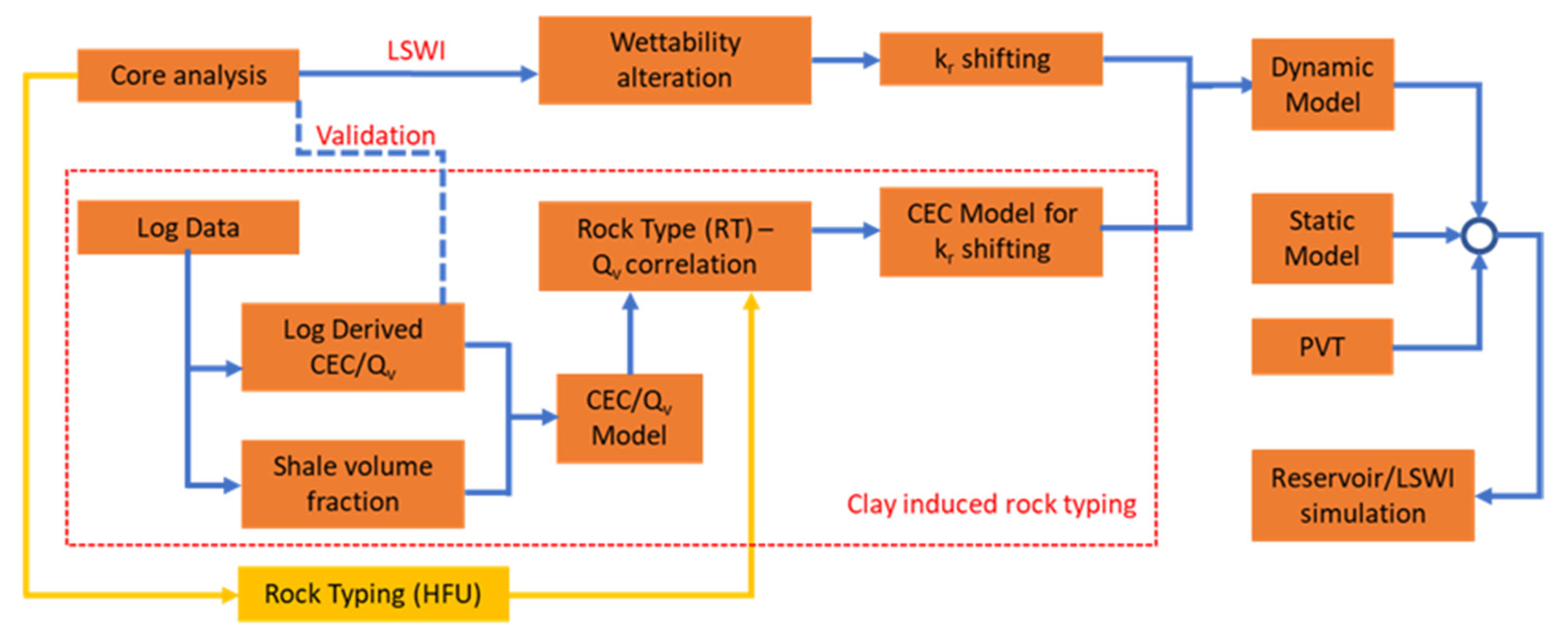
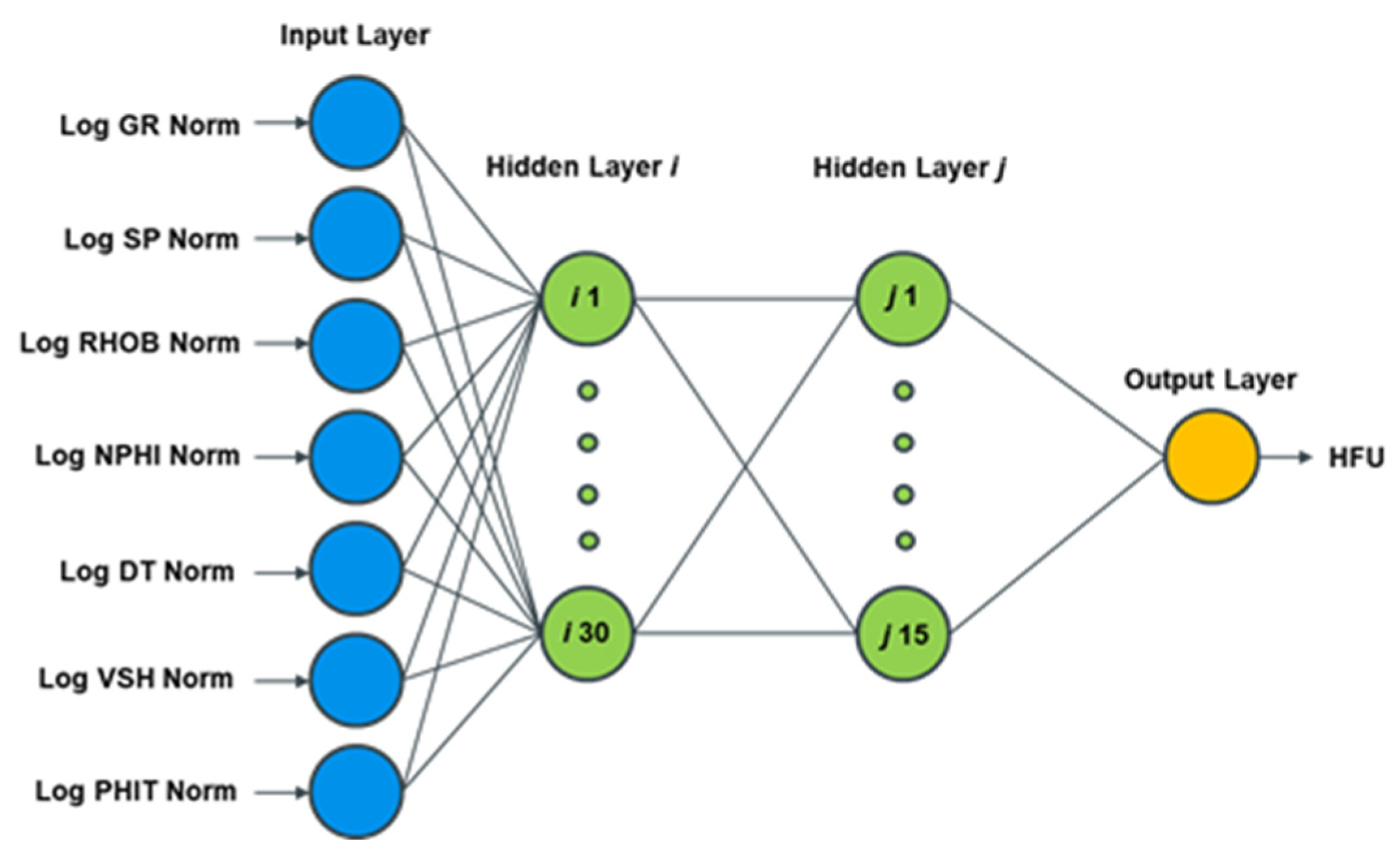
3. Methodology
4. Results and Discussion
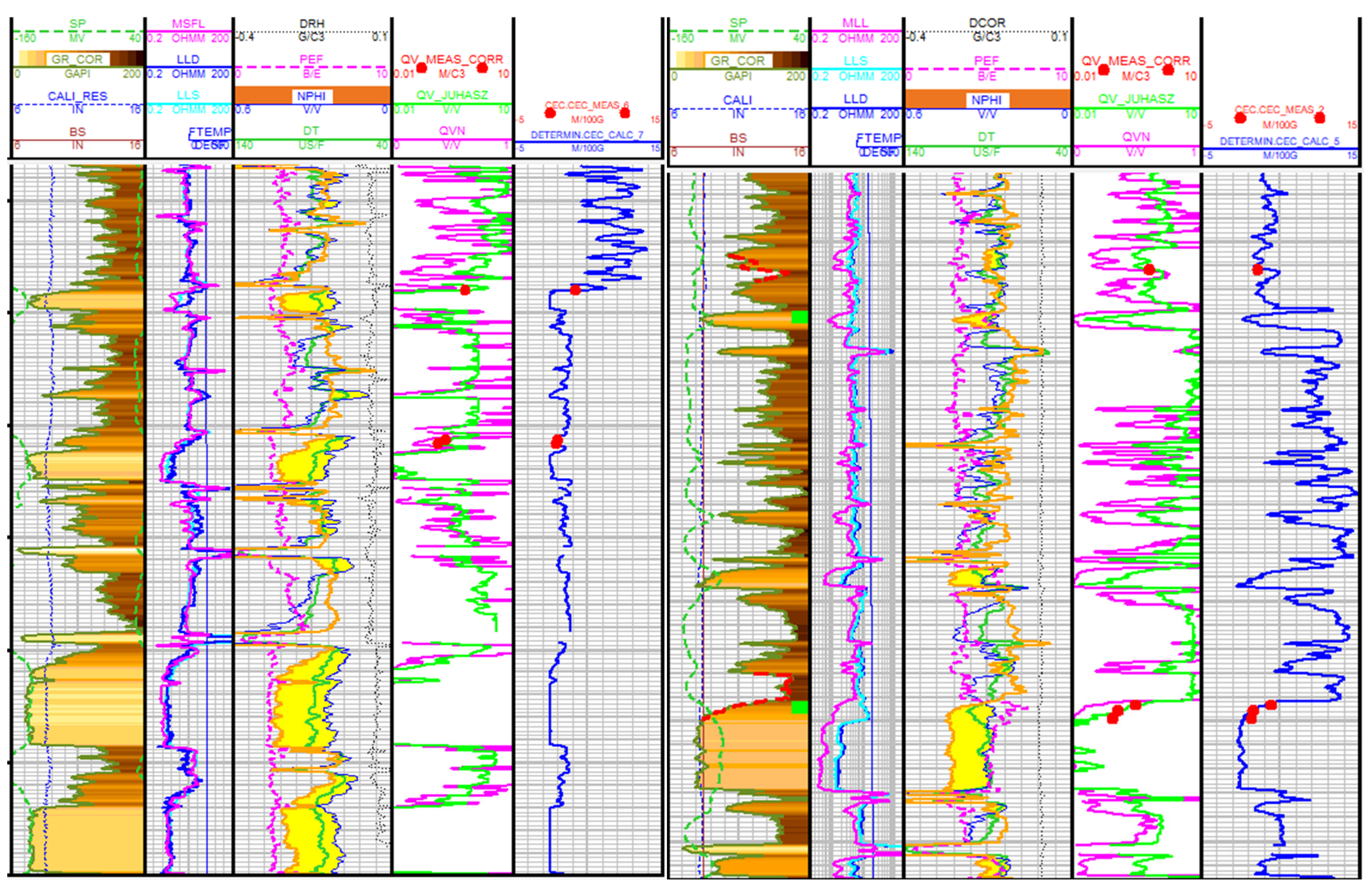
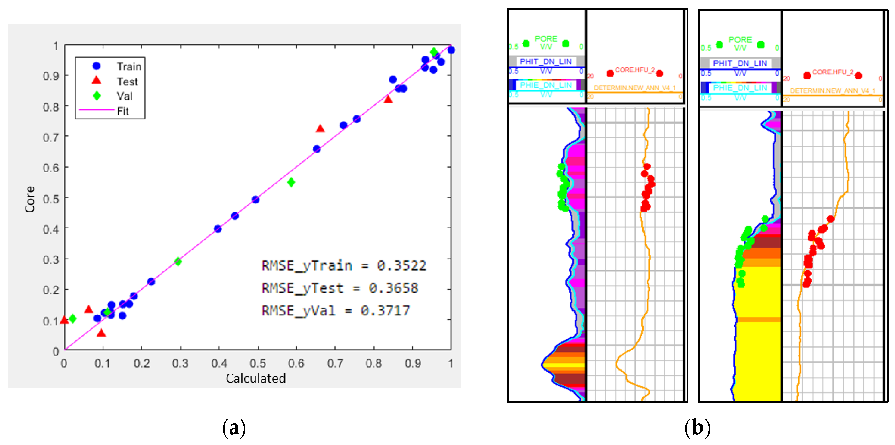
4.1. Log-Derived CEC Determination
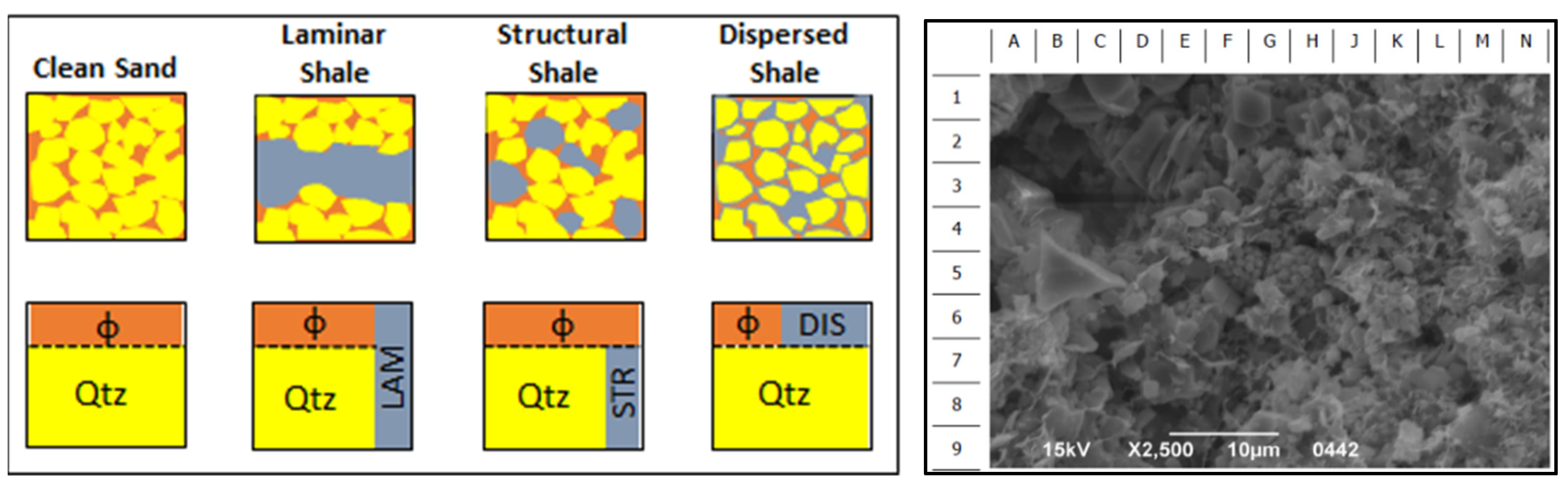
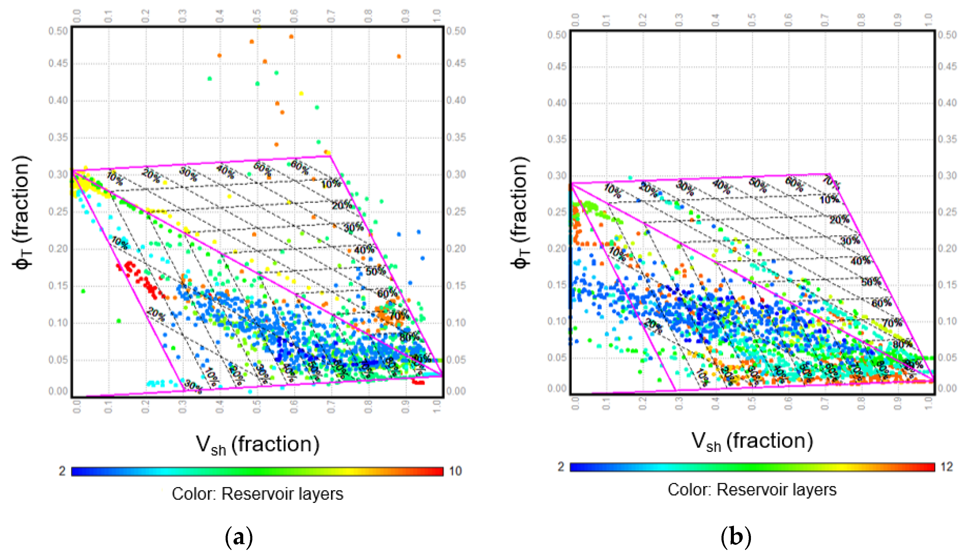
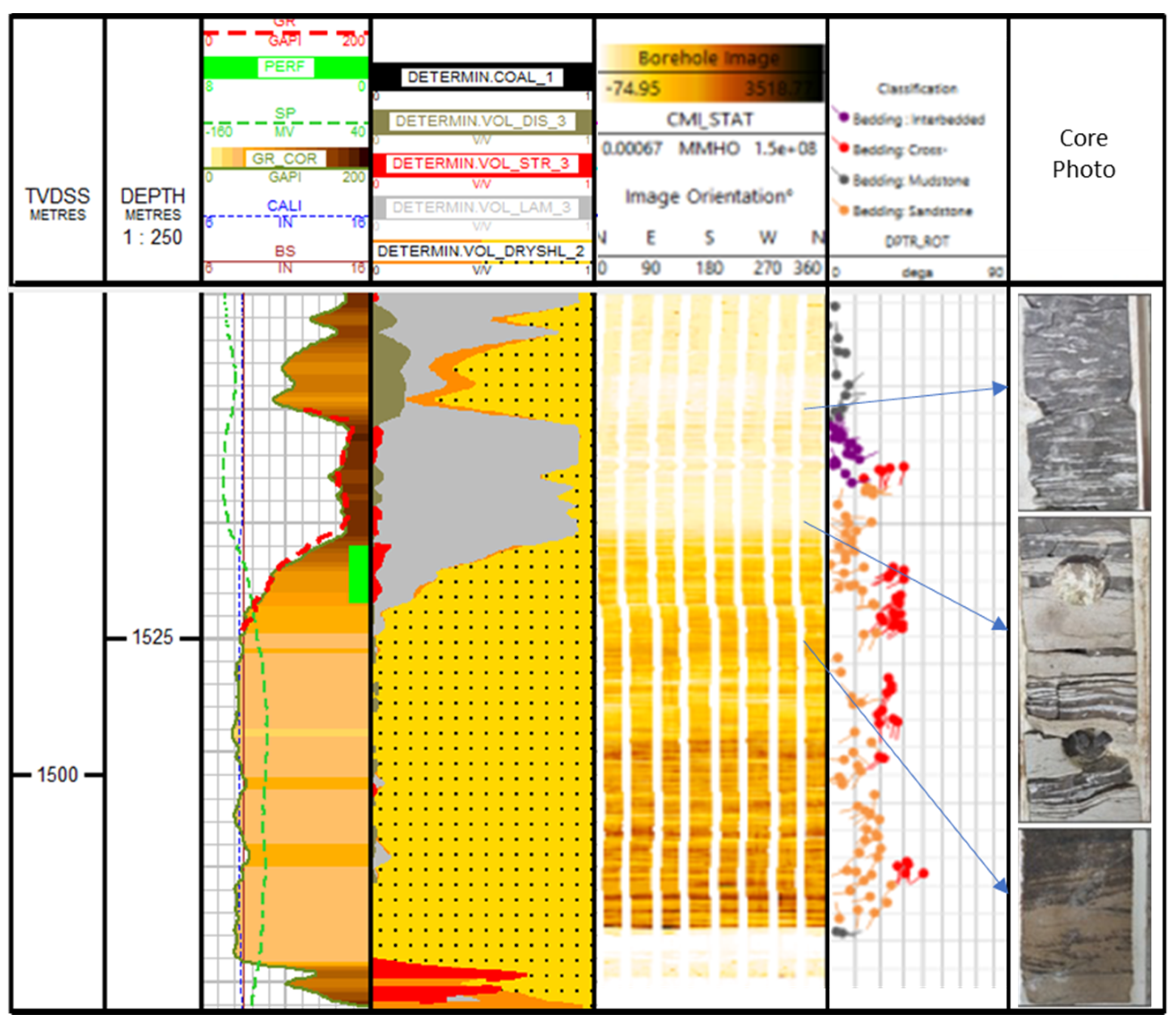
4.2. Clay Distribution
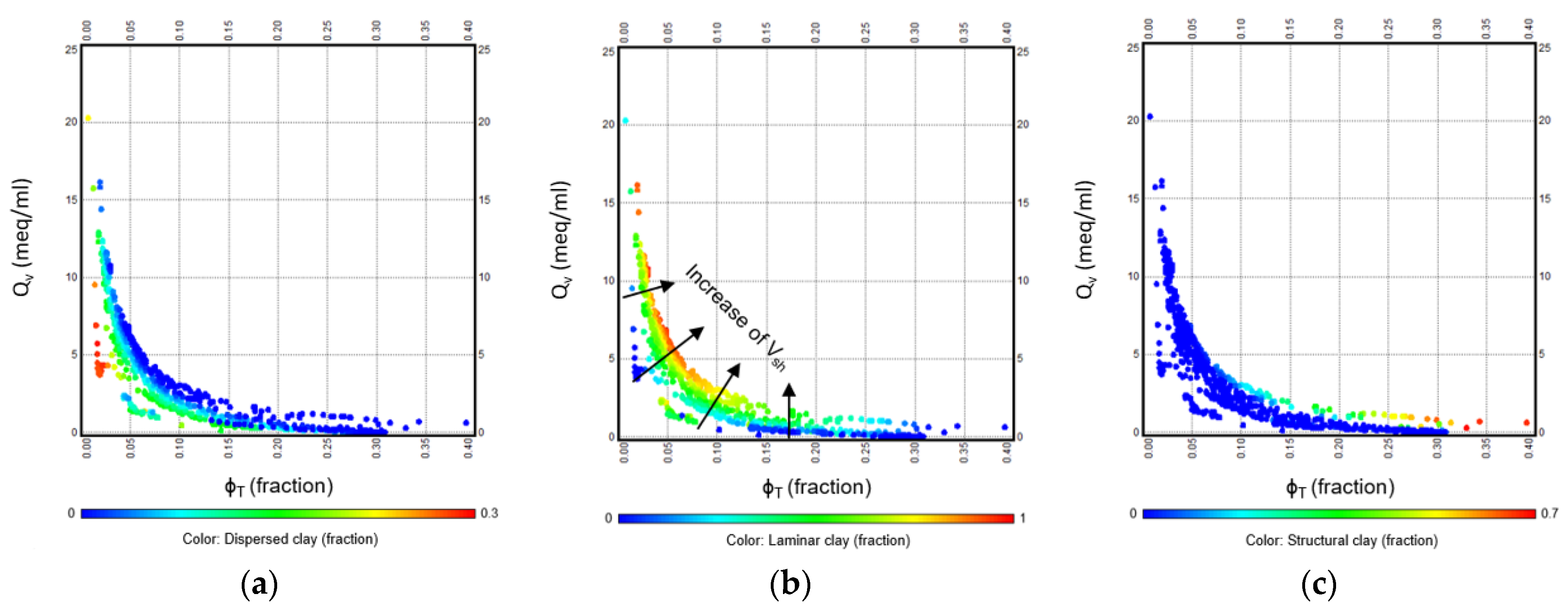
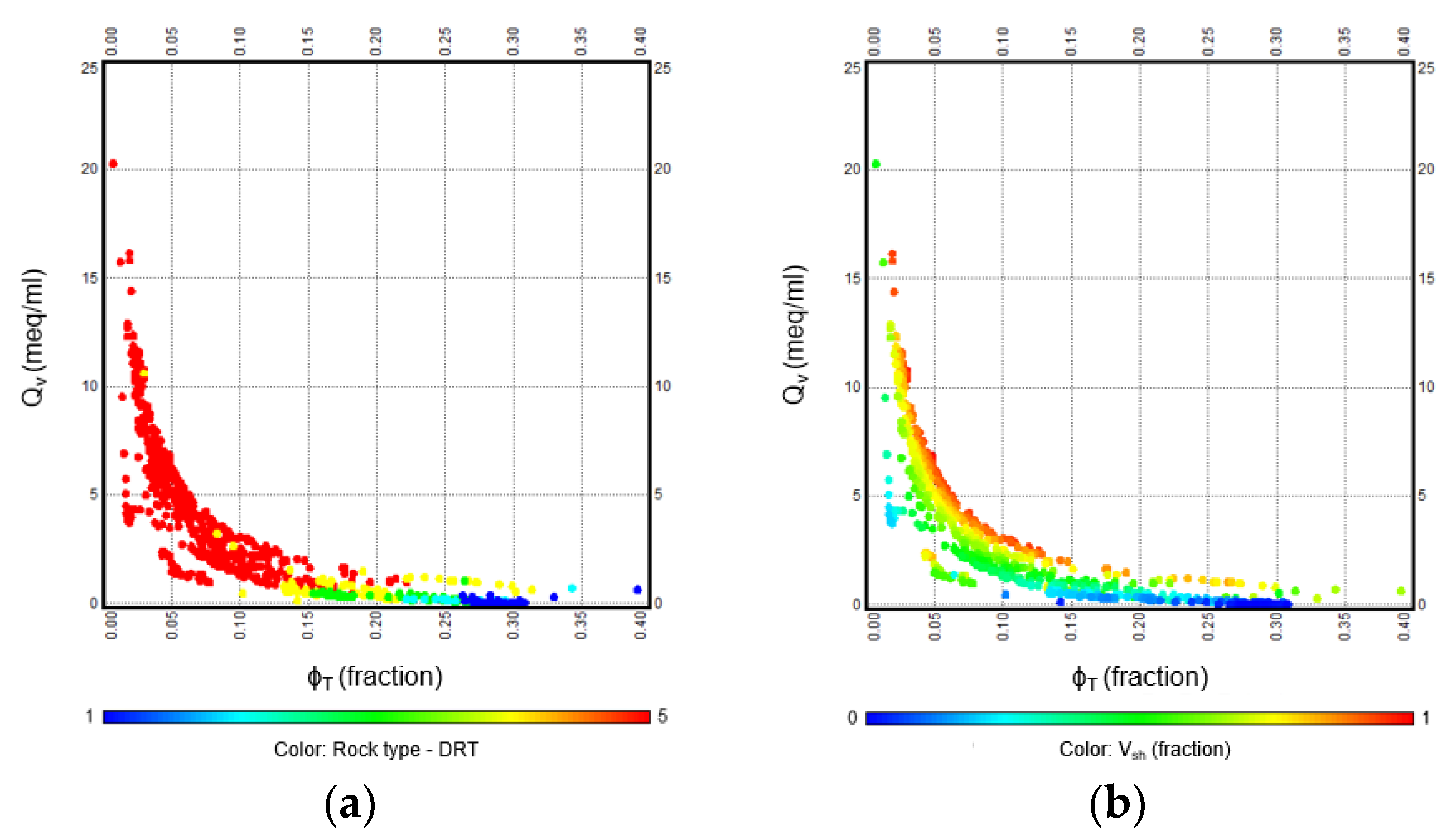
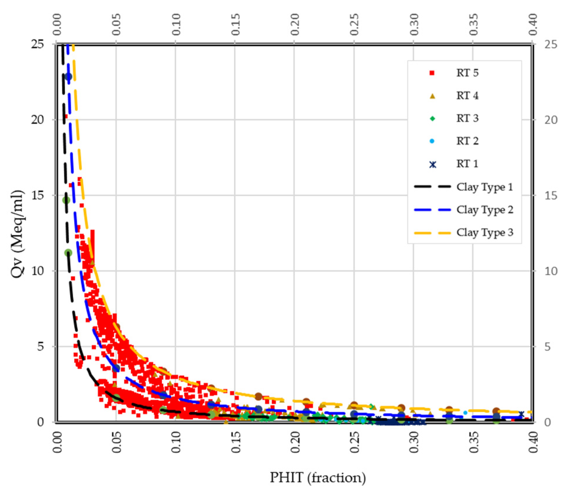
4.3. Relationship between Log-Derived Qv and Clay Distribution
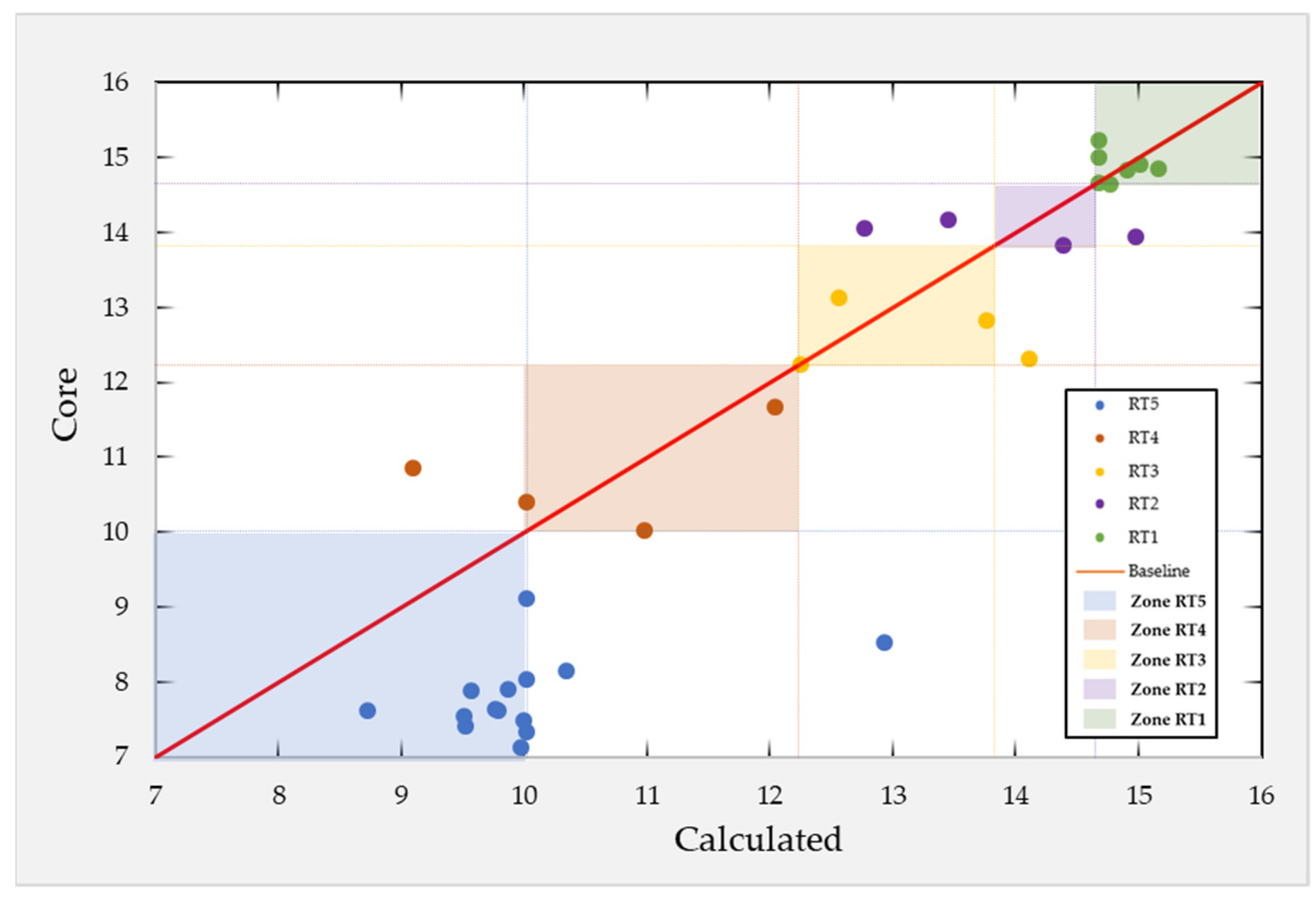
4.4. Log-Derived Rock Type Determination
4.5. Clay Induced Rock Typing
5. Conclusions
- An improved method was developed to characterize and classify the clay types by using the combination of log-derived cation exchange capacity and conventional rock types;
- The classification obtained by the clay typing method developed in this work can be utilized as an input for advanced modeling of low salinity water injection (LSWI) to provide more robust results. Previous studies simply used cation exchange capacity as a single input or were defined by empirical correlation;
- This work identifies that dispersed clay has a strong influence on the magnitude of cation exchange capacity rather than laminar and structural clays. Further investigation is strongly recommended to quantify the effects of clay distribution types and minerals on the clay typing method.
Author Contributions
Funding
Institutional Review Board Statement
Informed Consent Statement
Data Availability Statement
Acknowledgments
Conflicts of Interest
References
- Khormali, A.; Petrakov, D.G.; Lamidi, A.B.; Rastegar, R. Prevention of Calcium Carbonate Precipitation during Water Injection into High-Pressure High-Temperature Wells. In Proceedings of the SPE European Formation Damage Conference and Exhibition, Budapest, Hungary, 3–5 June 2015. [Google Scholar]
- Khormali, A.; Bahlakeh, G.; Struchkov, I.; Kazemzadeh, Y. Increasing inhibition performance of simultaneous precipitation of calcium and strontium sulfate scales using a new inhibitor—Laboratory and field application. J. Pet. Sci. Eng. 2021, 202, 109589. [Google Scholar] [CrossRef]
- Qiao, C.; Li, L.; Johns, R.T.; Xu, J. A mechanistic model for wettability alteration by chemically tuned waterflooding in carbonate reservoirs. SPE J. 2015, 20, 767–783. [Google Scholar] [CrossRef] [Green Version]
- Tang, G.Q.; Morrow, N.R. Influence of brine composition and fines migration on crude oil/brine/rock interactions and oil recovery. J. Pet. Sci. Eng. 1999, 24, 99–111. [Google Scholar] [CrossRef]
- McGuire, P.L.; Chatham, J.R.; Paskvan, F.K.; Sommer, D.M.; Carini, F.H. Low Salinity Oil Recovery: An Exciting New EOR Opportunity for Alaska’s North Slope. In Proceedings of the SPE Western Regional Meeting, Irvine, CA, USA, 30 March–1 April 2005. [Google Scholar]
- Austad, T.; RezaeiDoust, A.; Puntervold, T. Chemical Mechanism of Low Salinity Water Flooding in Sandstone Reservoirs. In Proceedings of the SPE Improved Oil Recovery Symposium, Tulsa, OK, USA, 24–28 April 2010. [Google Scholar]
- Lager, A.; Webb, K.J.; Collins, I.R.; Richmond, D.M. LoSal Enhanced Oil Recovery: Evidence of Enhanced Oil Recovery at the Reservoir Scale. In Proceedings of the SPE Symposium on Improved Oil Recovery, Tulsa, OK, USA, 20–23 April 2008. [Google Scholar]
- Ligthelm, D.J.; Gronsveld, J.; Hofman, J.; Brussee, N.; Marcelis, F.; van der Linde, H. Novel Waterflooding Strategy by Manipulation of Injection Brine Composition. In Proceedings of the EUROPEC/EAGE Conference and Exhibition, Amsterdam, The Netherlands, 8–11 June 2009. [Google Scholar]
- Dang, C.T.Q.; Nghiem, L.X.; Nguyen, N.; Chen, Z.; Nguyen, Q.P. Modeling and Optimization of Low Salinity Waterflood. In Proceedings of the SPE Reservoir Simulation Symposium, Houston, TX, USA, 23–25 February 2015. [Google Scholar]
- Ipek, G.; Bassiouni, Z.; Kurniawan, B.; Smith, J.R. Log-Derived Cation Exchange Capacity of Shaly Sands: Application to Hydrocarbon Detection. In Proceedings of the Petroleum Society’s 6th Canadian International Petroleum Conference (56th Annual Technical Meeting), Calgary, AB, Canada, 7–9 June 2005. [Google Scholar]
- Thomas, E.C.; Stieber, S.J. The Distribution of Shale in Sandstones and Its Effect upon Porosity. In Proceedings of the SPWLA 16th Annual Logging Symposium, New Orleans, LA, USA, 4–7 June 1975. [Google Scholar]
- Waxman, M.H.; Smits, L.J.M. Electrical conductivities in oil-bearing shaly sands. SPE J. 1968, 8, 107–122. [Google Scholar] [CrossRef]
- Juhasz, I. Normalised Qv—The Key to Shaly Sand Evaluation Using the Waxman-Smits Equation in the Absence of Core Data. In Proceedings of the SPWLA 22nd Annual Logging Symposium, Mexico City, Mexico, 23–26 June 1981. [Google Scholar]
- Ipek, G. Log-Derived Cation Exchange Capacity of Shaly Sands: Application to Hydrocarbon Detection and Drilling Optimization. Ph.D. Thesis, Louisiana State University, Baton Rouge, LA, USA, 2002. [Google Scholar]
- Demircan, G.; Smith, J.R.; Bassiouni, Z. Estimation of Shale Cation Exchange Capacity Using Log Data: Application to Drilling Optimization. In Proceedings of the SPWLA 41st Annual Logging Symposium, Dallas, TX, USA, 4–7 June 2000. [Google Scholar]
- Jerauld, G.R.; Lin, C.Y.; Webb, K.J.; Seccombe, J.C. Modeling low-salinity waterflooding. SPE Res. Eval. Eng. 2008, 11, 1000–1012. [Google Scholar] [CrossRef]
- Seilsepour, M.; Rashidi, M. Prediction of soil based on some soil physical and chemical properties. World App. Sci. J. 2008, 3, 200–205. [Google Scholar]
- Omekeh, A.V.; Evje, S.; Fjelde, I.; Friis, H.A. Experimental and Modeling Investigation of Ion Exchange during Low Salinity Waterflooding. In Proceedings of the International Symposium of the Society of Core Analysts, Austin, TX, USA, 18–21 September 2011. [Google Scholar]
- Fjelde, I.; Asen, S.M.; Omekeh, A. Low Salinity Water Flooding Experiments and Interpretation by Simulations. In Proceedings of the SPE Improved Oil Recovery Symposium, Tulsa, OK, USA, 14–18 April 2012. [Google Scholar]
- Dang, C.T.; Nghiem, L.X.; Chen, Z.; Nguyen, Q.P. Modeling Low Salinity Waterflooding: Ion Exchange, Geochemistry and Wettability Alteration. In Proceedings of the SPE Annual Technical Conference and Exhibition, New Orleans, LA, USA, 30 September–2 October 2013. [Google Scholar]
- Ginger, D.; Fielding, K. The Petroleum Systems and Future Potential of The South Sumatra Basin. In Proceedings of the Indonesian Petroleum Association 30th Annual Convention and Exhibition, Jakarta, Indonesia, 30 August–1 September 2005. [Google Scholar]
- Juhasz, I. Assessment of the Distribution of Shale, Porosity and Hydrocarbon Saturation in Shaly Sands. In Proceedings of the 10th European Formation Evaluation Symposium, Aberdeen, Scotland, UK, 22–25 April 1986. [Google Scholar]
- Amaefule, J.O.; Altunbay, M.; Tiab, D.; Kersey, D.G.; Keelan, D.K. Enhanced Reservoir Description: Using Core and Log Data to Identify Hydraulic (Flow) Units and Predict Permeability in Uncored Intervals/Wells. In Proceedings of the SPE Annual Technical Conference and Exhibition, Houston, TX, USA, 3–6 October 1993. [Google Scholar]
- Guo, G.; Diaz, M.A.; Paz, F.; Smalley, J.; Waninger, E.A. Rock typing as an effective tool for permeability and water-saturation modeling: A case study in a clastic reservoir in the oriente basin. SPE Res. Eval. Eng. 2007, 10, 730–739. [Google Scholar] [CrossRef]
- da Silva, M.L.; Martins, J.L.; Ramos, M.M.; Bijani, R. Estimation of clay minerals from an empirical model for cation exchange capacity: An example in Namorado oilfield, Campos Basin, Brazil. Appl. Clay Sci. 2018, 158, 195–203. [Google Scholar] [CrossRef]


| Well | Sample Number | Depth (Meter) | Porosity (%) | Permeability (mD) | Grain Density (gr/cc) | CEC (meq/100gr) | Qv (meq/mL) | Total Clay (%) | Mineral Clay Prediction (XRD) |
|---|---|---|---|---|---|---|---|---|---|
| B-4 | 8 | 1509.20 | 13.61 | 1.92 | 2.64 | 1.60 | 0.27 | 10.0 | Clean |
| 9 | 1511.00 | 17.24 | 94.87 | 2.64 | 1.20 | 0.15 | 26.0 | Kaolinite, Illite | |
| 13A | 1570.00 | 6.41 | 0.08 | 2.65 | 3.40 | 1.32 | 50.0 | Kaolinite, Illite | |
| 14A | 1571.00 | 7.64 | 0.06 | 2.65 | 14.40 | 4.61 | 32.0 | Kaolinite, Illite, Clorite | |
| 19A | 1603.40 | 9.26 | 1.25 | 2.66 | 1.00 | 0.26 | 10.0 | Clean | |
| 20 | 1604.20 | 11.84 | 75.29 | 2.64 | 0.80 | 0.16 | 17.0 | Clean | |
| B-5 | 3A | 1431.78 | 15.50 | 0.38 | 2.66 | 2.19 | 0.32 | 20.8 | Kaolinite, Illite, Clorite |
| 12C | 1522.92 | 20.00 | 64.70 | 2.65 | 3.91 | 0.41 | 14.1 | Kaolinite, Illite | |
| 13B | 1523.44 | 22.70 | 704.00 | 2.65 | 1.62 | 0.15 | 25.0 | Kaolinite, Illite | |
| 14C | 1524.73 | 26.10 | 2360.00 | 2.65 | 1.37 | 0.10 | 17.4 | Clean |
| NxRD | NxGR | NxRHO | NxNPHI | NxSP | NxDT | ||
|---|---|---|---|---|---|---|---|
| Coeff. label | |||||||
| Coeff. value | 9.766 | 15.894 | −6.532 | −4.867 | 11.023 | 0.676 | 7.177 |
| Correlations | Implementation in RT 1–3 | Implementation in RT 4–5 | RMSE | |
|---|---|---|---|---|
| Clay type 1 | - | Vsh: 0–0.125 | 0.289 | |
| Clay type 2 | All range of Vsh | Vsh: 0.126–0.875 | 1.356 | |
| Clay type 3 | - | Vsh: 0.876–1 | 1.289 |
Publisher’s Note: MDPI stays neutral with regard to jurisdictional claims in published maps and institutional affiliations. |
© 2022 by the authors. Licensee MDPI, Basel, Switzerland. This article is an open access article distributed under the terms and conditions of the Creative Commons Attribution (CC BY) license (https://creativecommons.org/licenses/by/4.0/).
Share and Cite
Zakyan, H.; Permadi, A.K.; Pratama, E.A.; Naufaliansyah, M.A. An Improved Method of Clay-Induced Rock Typing Derived from Log Data in Modelling Low Salinity Water Injection: A Case Study on an Oil Field in Indonesia. Energies 2022, 15, 3749. https://0-doi-org.brum.beds.ac.uk/10.3390/en15103749
Zakyan H, Permadi AK, Pratama EA, Naufaliansyah MA. An Improved Method of Clay-Induced Rock Typing Derived from Log Data in Modelling Low Salinity Water Injection: A Case Study on an Oil Field in Indonesia. Energies. 2022; 15(10):3749. https://0-doi-org.brum.beds.ac.uk/10.3390/en15103749
Chicago/Turabian StyleZakyan, Hafizh, Asep Kurnia Permadi, Egi Adrian Pratama, and Muhammad Arif Naufaliansyah. 2022. "An Improved Method of Clay-Induced Rock Typing Derived from Log Data in Modelling Low Salinity Water Injection: A Case Study on an Oil Field in Indonesia" Energies 15, no. 10: 3749. https://0-doi-org.brum.beds.ac.uk/10.3390/en15103749