Control Design and Parameter Tuning for Islanded Microgrids by Combining Different Optimization Algorithms

Abstract

Load and supply parameters may be uncertain in microgrids (MGs) due for instance to the intermittent nature of renewable energy sources among others. Guaranteeing reliable and stable MGs despite parameter uncertainties is crucial for their correct operation. Their stability and dynamical features are directly related to the controllers’ parameters and power-sharing coefficients. Hence, to maintain power good quality within the desirable range of system parameters and to have a satisfactory response to sudden load changes, careful selection of the controllers and power-sharing coefficients are necessary. In this paper, a simple design approach for the optimal design of controllers’ parameters is presented in an islanded MG. To that aim, an optimization problem is formulated based on a small-signal state-space model and solved by three different optimization techniques including particle swarm optimization (PSO), genetic algorithm (GA), and a proposed approach based on the combination of both PSO and GA. The optimized coefficients are selected to guarantee desirable static and dynamic responses in a wide range of operations regardless of the number of inverters, system configuration, output impedance differences, and load types. Through the proposed design and tuning method, the performance of the MG is improved as compared to those obtained using state-of-art techniques. This fact is demonstrated by using numerical simulations performed on a detailed model implemented in PSIM^© software.

1. Introduction

With the use of distributed renewable energy sources that can be utilized locally to produce and feed electric power, the concept of microgrids (MGs) has emerged. The MGs have two operating modes: grid-connected and islanded mode [1]. The issue of power balance between production and consumption, which is equivalent to the load and frequency control has been one of the major challenges in the islanded mode of operation [2]. Imbalances between distributed generations (DGs) and loads in MGs create frequency fluctuation which leads to a decrease in power quality or even may put the system stability at risk [3]. Furthermore, high penetration of renewable energies in MGs can bring uncertainties due to unpredictable environmental changes in terms of solar irradiance, temperature, wind speed, etc. [4]. Therefore, a robust control technique is needed to guarantee the small-signal stability of MGs despite load or source changes. In the islanded mode of operation, the most usable controller is the PI corrector which is implemented in a two-loop hierarchical structure. Namely, power control is performed by an outer control loop with low bandwidth while an inner control loop with higher bandwidth than the outer loop is responsible for voltage and current control [5]. The responsibility of the inner current and voltage controller loops is to track voltage and current reference values during disturbances as well as to damp output filter resonances [6]. The aim of the outer loop is to guarantee active and reactive power-sharing with other DGs. Various types of power-sharing control strategies have been proposed in islanding operation of MGs [7], e.g., master/slave control [8], distributed control [9], and droop control [10]. Among them, the droop control strategy inspired by the behaviour of synchronous generators has more advantages such as the capability of applying in both modes of MG operations, needless communication lines among DGs, and plug-and-play functionality [11].

Based on the type of common bus voltages, MGs are classified into AC [12], DC [13] and hybrid AC/DC [14]. In the case of AC MGs, voltage-source inverters (VSI) are used as interfaces between the common bus voltage and the load. These VSIs have lower physical inertia in comparison with synchronous generators [15] which means that their dynamic response is much faster. This fast dynamic response makes them vulnerable in front of different disturbances. Therefore, for the reliable operation of MGs, small-signal stability is required in a wide range of operations [16]. The power quality and stability of MGs are affected by droop control coefficients and controllers’ parameters. 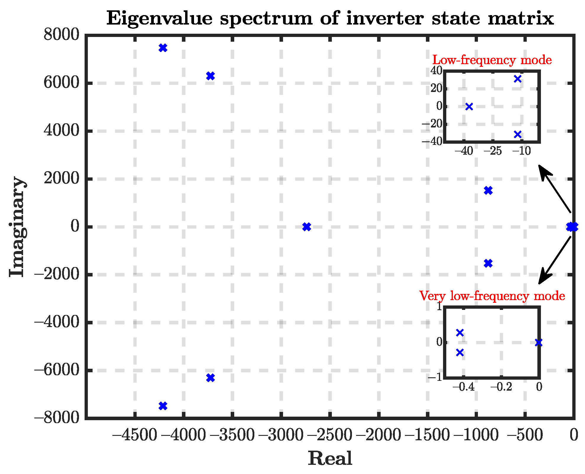In [17], it is proved, by using root locus and sensitivity analysis, that the low-frequency eigenvalues of the MG are strictly sensitive to the droop controller parameters. Therefore, the selection of controllers’ coefficients needs careful attention [18] to satisfy MG power quality conditions and smooth and stable operation during load changes. In addition, by optimally selecting these parameters, it is conceivable that the islanded MG can be stable in a wide range of operations with less voltage and frequency steady-state errors. Also, in [19], even with similar parallel inverters and identical parameters, the uncertainty brought by different output impedances might destabilize the system. Different approaches have been presented in the literature to select the controllers’ coefficients [20]. The most used ones are based on a trial and error approach which is time-consuming, especially in a complex MG and the tuned parameters are not the optimum ones. Furthermore, this approach does not provide a systematic guideline for the design of controllers’ coefficients in the MGs. Another approach is to design the controllers’ parameters in such a way that the dynamics of the outer loop be slower than that of the inner loop [21]. Under this assumption, the inner and outer control loops can be separately designed. Normally, the bandwidth of the outer loop is limited to $1/10$ of the inner loop [22]. However, this approach has similar disadvantages to the trial and error method. The last approach to design the controllers’ coefficients is to employ optimization algorithms such as genetic algorithm (GA) [23] and particle swarm optimization (PSO). They are widely used in the MGs for different areas, such as harmonic mitigation [24] and optimal scheduling [25]. The authors in [26] used the PSO algorithm to optimally select the MG control parameters. In their approach, the problem constraints are not exactly specified which can jeopardize the stability of the MG. In addition, the objective function can only remove the steady-state error of the active power. In [27] a two-layer PSO algorithm was used for parameter selection in the inverter side inductor current control theory framework. In that work, only the effect of PI controller parameters was investigated. However, the impact of power-sharing coefficients is also important and the choice of these parameters is critical [28]. In [29] an online intelligent method, based on the combination of fuzzy logic and PSO techniques, was proposed for the selection of PI parameters to control the MG frequency. In [30] Grasshopper Optimization Algorithm (GOA) was used, and in [31] PSO was used to tune the PI controller parameters. PSO was also used in [32] to design triple-action controllers’ parameters for an islanded AC MG. In [33], GA was used to design controller parameters in the secondary control level of an AC MG, and in [34] a non-dominated sorting genetic algorithm-II was used to design the parameters for the fractional order PID controller. However, the performance of GA shows premature convergence in some cases [35].

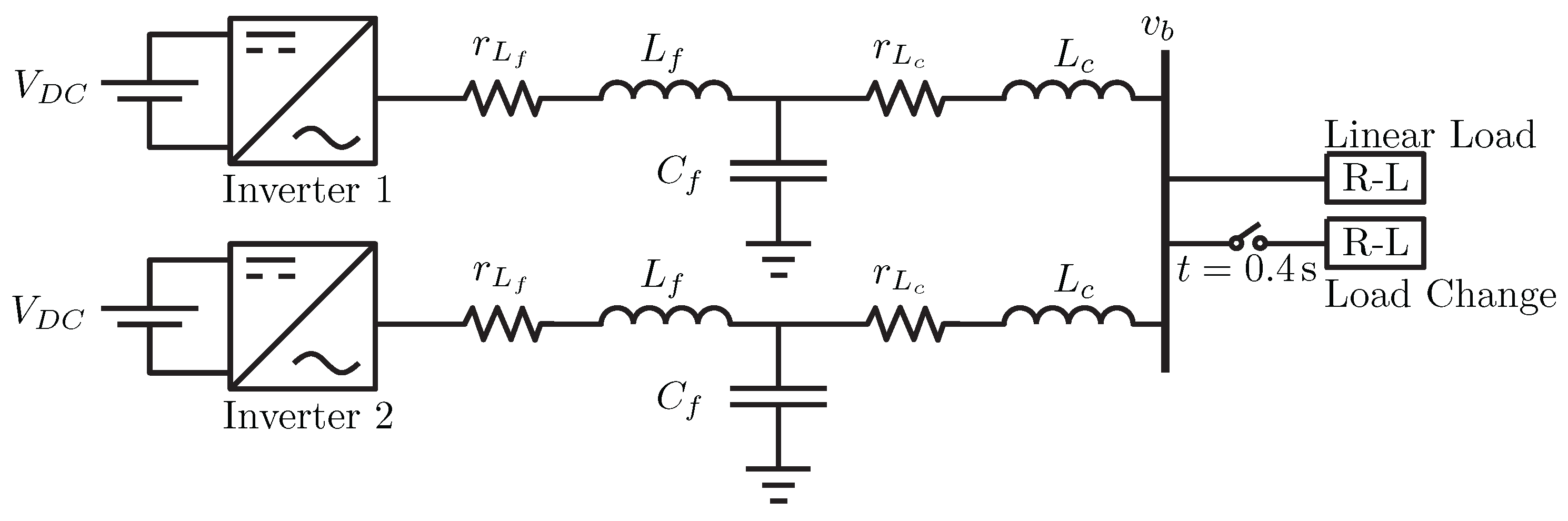
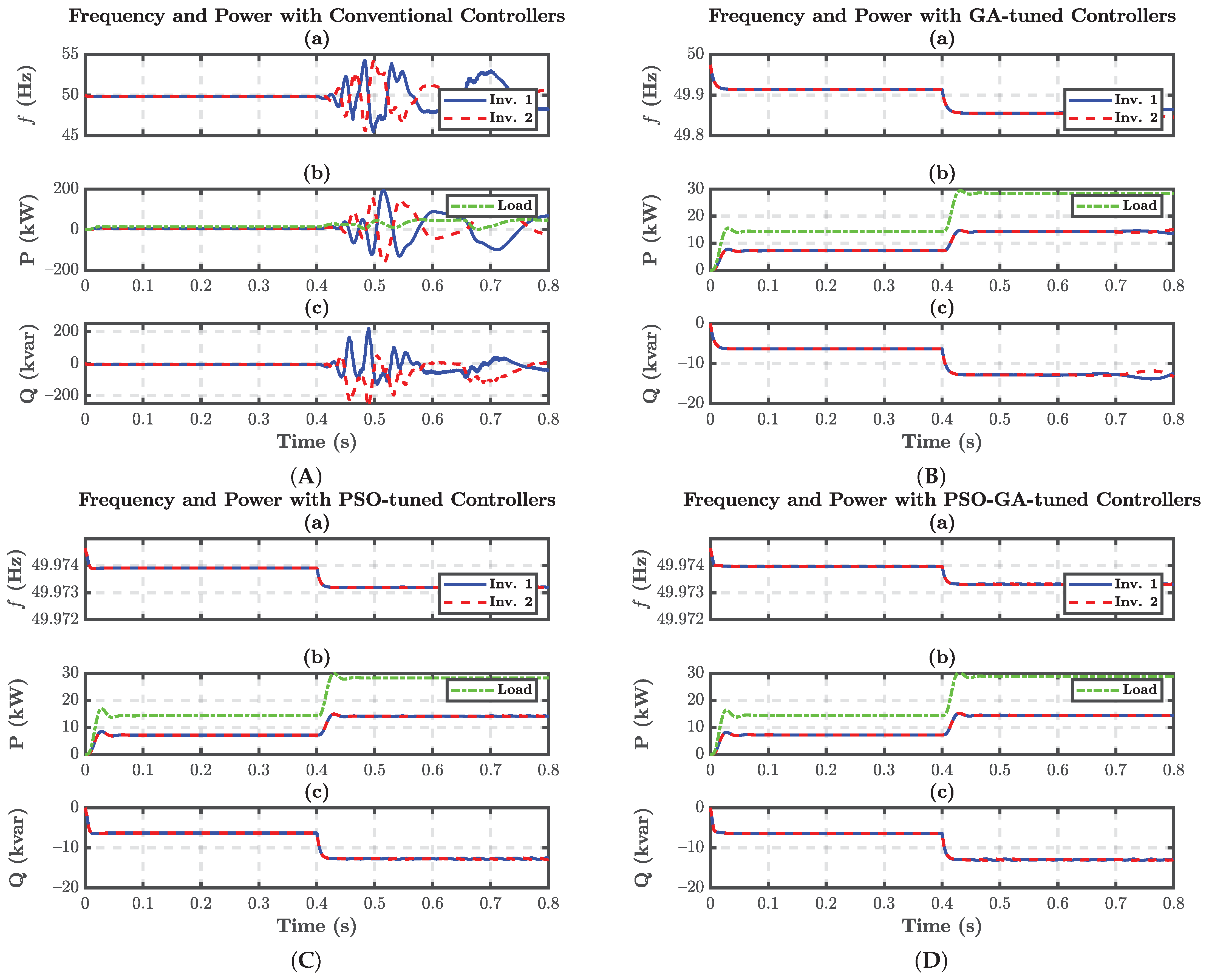
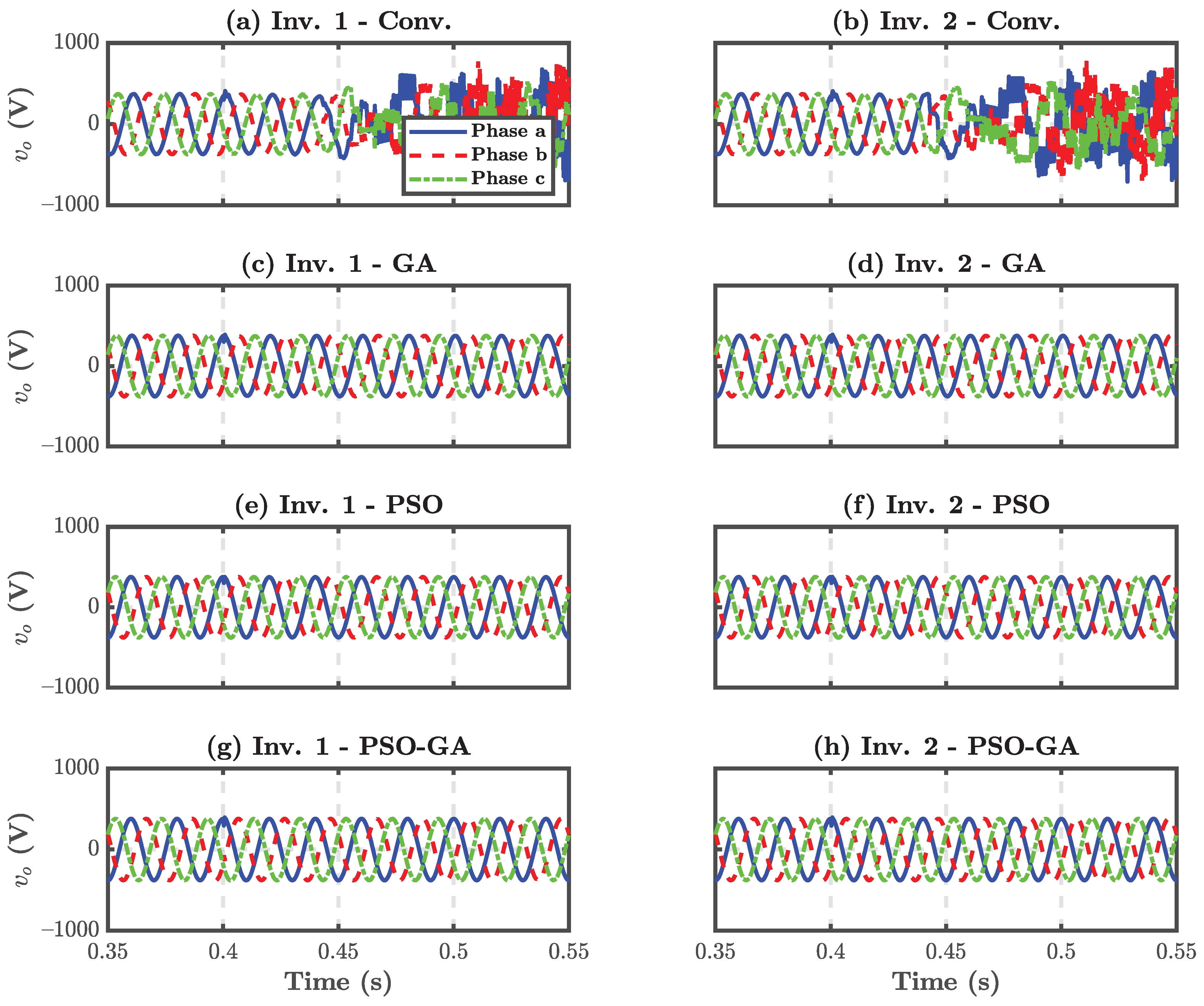
None of the above-mentioned references provides a universal and simple design approach to tune the controllers’ parameters which guarantees the small-signal stability in the whole range of operation. In this paper, regardless of the number of inverters, MG configuration, output line impedance, or types of loads, a straightforward design approach is presented. This can minimize designers’ efforts to the tuning MG controllers’ parameters when the output impedances, the number of inverters, and MG configuration may change. Since the VSIs are interfaced to a common bus voltage with huge coupling inductances and the distribution lines have resistive-inductive impedances, it can be concluded that the stable and optimal operation of each VSI can guarantee stable and optimal operation of the whole MG provided that interacting effects are neglected. Therefore, in the proposed design approach, the small signal analysis of a VSI is considered. A novel eigenvalues-based objective function is defined which involves stability criteria eliminating the need of performing sophisticated stability analysis and making the control design method simpler than traditional techniques. Power controller coefficients, PI current and voltage controller gains are determined through the optimization problem which is solved through different algorithms such as PSO, GA, and proposed PSO-GA intending to improve both system static and dynamic performances. The proposed combined PSO-GA uses both PSO and GA. The controllers’ coefficients can be determined off-line for the worst-case scenario of the operating point. In order to validate the proposed method, different case studies including load changes in the two-inverter system are simulated in the islanded mode of operation using PSIM^© software. A comparative analysis among optimization algorithms is carried out for the different case studies. The main contributions of the paper are listed below.

• Proposing a new simple design approach and tuning method for the optimal setting of power, voltage, and current controllers’ coefficients.
• Proposing novel objective function evaluating optimized parameters for the controllers while ensuring the VSI stability in the whole range of operation.
• Proposing a combination of PSO and GA for parameter tuning for a VSI in an MG application.

The rest of this paper is organized as follows. In, Section 2, a complete small-signal model of the VSI inverter in an MG application is derived. Section 3 is devoted to defining the proposed design approach and formulating the optimization problem which is solved through GA, PSO, and the proposed PSO-GA algorithm. Section 4 presents simulation results for different case studies. Section 5 concludes the paper.

2. State-Space Modelling of the Inverter

Figure 1 shows the control schematic diagram of a VSI in an islanded MG. The used control strategy consists of power, voltage, and current controllers in a hierarchical structure. The current controller is the fastest one and the power controller is the slowest one. The control is implemented in the $dq$ reference frame. The most appropriate and simplest controller in this frame is a PI controller [36] which is used in this study, for both current and voltage loops. For the power controller, the droop control method is employed.

As the inverter is connected to the AC common bus through an inductor ($L_c$), the power control can be carried out by using two artificial linear characteristics in the inverter frequency and voltage as shown in Figure 2. The frequency is set based on droop gain $m_p$ and the voltage is set according to the droop gain $n_q$. The inverter phase can be determined by integrating the frequency. Droop control technique arises from synchronous generator governor and inertia characteristics. As an example, when the generator has drawn, power increases, and the rotation speed decreases [37]. Therefore, MG active and reactive power can be controlled in the $dq$ reference frame by manipulating inverter output voltage magnitude and frequency as follows:

$$\left\{\begin{array}{cc}\hfill \omega & ={\omega }_n-m_{p}P\hfill \\ \hfill v_{od}^{\ast }& =V_n-n_{q}Q\hfill \\ \hfill v_{oq}^{\ast }& =0\hfill \end{array}\right.$$

(1)

where ${\omega }_n$ and $V_n$ are the nominal frequency and voltage respectively. P and Q are the DC components of instantaneous active and reactive power. It should be noted that in presence of more than one inverter in the MG, to build the complete small-signal model, the rotation speed of one inverter $\delta$ should be considered as a reference frame. Then, all other inverters’ rotation speeds should translate to the one which is considered as a reference. Figure 3 illustrates the block diagram of the control scheme in $dq$ reference frame. First, measured currents and voltages go through the $dq$ transform block. Then, DC values of active and reactive power are calculated with a low pass filter. The low pass filter is used to guarantee the proper current sharing of nonlinear loads [38]. According to the $dq$ synchronous reference frame theory, harmonic components will appear in the nonlinear load active and reactive power. These should be removed from the DC values. The DC values of active and reactive power enter the frequency and voltage droop loops and build the rotation angle and d-axis voltage reference value for the outer voltage controllers. The q-axis voltage reference value is set to zero. Thereafter, the outputs of PI voltage controllers plus a portion of $dq$-axis voltages and $dq$-axis output currents make the reference value of inner current controllers. The calculated reference value for the inverter voltage goes through an inverse $dq$ transform block to build three-phase signals for the inverter pulse width modulation.

A complete small-signal model of an islanded MG, which is detailed by [17,39], is briefly presented here. Combining the state-space model of power, voltage, and current controllers and linearizing the models at the operating point yields to (2).

$$\left[\begin{array}{c}\dot{\Delta \delta }\\ \dot{\Delta P}\\ \dot{\Delta Q}\\ \dot{\Delta {\varphi }_d}\\ \dot{\Delta {\varphi }_q}\\ \dot{\Delta {\psi }_d}\\ \dot{\Delta {\psi }_q}\\ \dot{\Delta i_{ld}}\\ \dot{\Delta i_{lq}}\\ \dot{\Delta v_{od}}\\ \dot{\Delta v_{oq}}\\ \dot{\Delta i_{od}}\\ \dot{\Delta i_{oq}}\end{array}\right]=\left[\begin{array}{ccccccccccccc}0& -m_p& 0& 0& 0& 0& 0& 0& 0& 0& 0& 0& 0\\ 0& -{\omega }_c& 0& 0& 0& 0& 0& 0& 0& {\omega }_c{I}_{od}& {\omega }_c{I}_{oq}& {\omega }_c{V}_{od}& {\omega }_c{V}_{oq}\\ 0& 0& -{\omega }_c& 0& 0& 0& 0& 0& 0& {\omega }_c{I}_{oq}& -{\omega }_c{I}_{od}& -{\omega }_c{V}_{oq}& {\omega }_c{V}_{od}\\ 0& 0& -n_q& 0& 0& 0& 0& 0& 0& -1& 0& 0& 0\\ 0& 0& 0& 0& 0& 0& 0& 0& 0& 0& -1& 0& 0\\ 0& 0& -n_q{K}_{pv}& K_{iv}& 0& 0& 0& -1& 0& -K_{pv}& -{\omega }_n{C}_f& F& 0\\ 0& 0& 0& 0& K_{iv}& 0& 0& 0& -1& {\omega }_n{C}_f& -K_{pv}& 0& F\\ 0& -m_p{I}_{lq}& \frac{-n_q{K}_{pc}{K}_{pv}}{L_f}& \frac{K_{pc}{K}_{iv}}{L_f}& 0& \frac{K_{ic}}{L_f}& 0& \frac{-r_{L_f}-K_{pc}}{L_f}& {\omega }_0-{\omega }_n& \frac{-K_{pc}{K}_{pv}-1}{L_f}& \frac{-{\omega }_n{C}_f{K}_{pc}}{L_f}& \frac{F{K}_{pc}}{L_f}& 0\\ 0& m_p{I}_{ld}& 0& 0& \frac{K_{pc}{K}_{iv}}{L_f}& 0& \frac{K_{ic}}{L_f}& {\omega }_n-{\omega }_0& \frac{-r_{L_f}-K_{pc}}{L_f}& \frac{{\omega }_n{C}_f{K}_{pc}}{L_f}& \frac{-K_{pc}{K}_{pv}-1}{L_f}& 0& \frac{F{K}_{pc}}{L_f}\\ 0& -m_p{V}_{oq}& 0& 0& 0& 0& 0& \frac{1}{C_f}& 0& 0& {\omega }_0& -\frac{1}{C_f}& 0\\ 0& m_p{V}_{od}& 0& 0& 0& 0& 0& 0& \frac{1}{C_f}& -{\omega }_0& 0& 0& -\frac{1}{C_f}\\ \frac{-V_{bq}}{L_c}& -m_p{I}_{oq}& 0& 0& 0& 0& 0& 0& 0& \frac{1}{L_c}& 0& -\frac{r_{L_c}}{L_c}& {\omega }_0\\ \frac{-V_{bd}}{L_c}& m_p{I}_{od}& 0& 0& 0& 0& 0& 0& 0& 0& \frac{1}{L_c}& -{\omega }_0& -\frac{r_{L_c}}{L_c}\end{array}\right]\left[\begin{array}{c}\Delta \delta \\ \Delta P\\ \Delta Q\\ \Delta {\varphi }_d\\ \Delta {\varphi }_q\\ \Delta {\psi }_d\\ \Delta {\psi }_q\\ \Delta i_{ld}\\ \Delta i_{lq}\\ \Delta v_{od}\\ \Delta v_{oq}\\ \Delta i_{od}\\ \Delta i_{oq}\end{array}\right]$$

(2)

In (2), ${\varphi }_d$, ${\varphi }_q$, ${\psi }_d$, and ${\psi }_q$ are the state variables of current and voltage controllers. $V_{bd}$, $V_{bq}$, $I_{ld}$, $I_{lq}$, $I_{od}$, $I_{oq}$, $V_{od}$, $V_{oq}$ are the operating points of the MG and ${\omega }_c$ is the cut-off frequency of power controller. $K_{pv},K_{iv},K_{pc},K_{ic}$ are the proportional and the integral gains of the voltage and current controllers respectively while F is the gain of dynamic improvement loop. As it is shown in (2), the state matrix for an islanded MG with only one inverter has $13\times 13$ dimension. Therefore, it has 13 eigenvalues and their locus in the complex plain are shown in Figure 4.

The comparison of the small-signal average model of the islanded MG with one inverter and the large-signal switched model is shown in Figure 5. The islanded MG operation point changes from a normal one to another operating condition with 100% load step change.

3. Proposed Design Approach

In this section, the proposed design approach of controllers’ coefficients is presented. The design approach is formulated as an optimization problem to find the best-fitted values for the control system coefficients $\left[m_p{n}_q{K}_{pv}{K}_{iv}{K}_{pc}{K}_{ic}\right]$. The optimization problem is solved through different optimization techniques including PSO, GA, and the proposed PSO-GA which is the combination of PSO and GA.

3.1. Formulation of Optimization Problem

The aim of minimising the objective function is to improve system dynamic behaviour and damping characteristics as well as to keep the stability of the whole system under load changes. This can be done by making all the eigenvalues of the state matrix with a damping ratio close to an appropriate value [40]. The selection of damping ratio is to make a trade-off between magnitude and time of system overshoot. Therefore damping ratio selection is a subjective choice and is usually selected between $0.4$ and $0.7$. As it is mentioned previously, the state matrix of the inverter has 13 eigenvalues all can be expressed as follows

$$s=-\zeta {\omega }_n\pm j{\omega }_n\sqrt{1-{\zeta }^2}$$

(3)

where $\zeta$ and ${\omega }_n$ are the modes damping ratio and natural frequency. In this paper, the objective function is selected in such a way that all the 13 system eigenvalues are such that the damping ratio is $0.5$. Another important thing is the stability of the closed-loop system with PI controllers. To have a stable system, a term is added to the objective function to guarantee the stability of the whole system with designed controller parameters. This term is $\mathtt{i}\mathtt{s}\mathtt{s}\mathtt{t}\mathtt{a}\mathtt{b}\mathtt{l}\mathtt{e}\left(\right)$ function in MATLAB environment which returns zero when a state matrix is unstable and returns one when it is stable. Adding this term to the objective function eases the stability analysis of the system. Therefore, the resulted parameters through all optimization algorithms guarantee the stability of the whole system. The definition of the objective function is illustrated in the following equation

$$\mathrm{Objective}\mathrm{Function}=-\mathtt{i}\mathtt{s}\mathtt{s}\mathtt{t}\mathtt{a}\mathtt{b}\mathtt{l}\mathtt{e}\left(\mathrm{state}\mathrm{matrix}\right)+\sqrt{\frac{{\displaystyle \sum _{i=1}^{13}}{({\zeta }_i-0.5)}^2}{13\times 0.25}}$$

(4)

where in the denominator of the objective function second term, $13\times 0.25$ would normalize the value between 0 and 1 [41].

3.2. Proposed PSO-GA

The proposed optimization technique is the combination of two powerful optimization algorithms, PSO and GA, and is called here PSO-GA. The proposed PSO-GA provides both powers of PSO and GA in one optimization algorithm. PSO has the ability to traverse the search space continuously like birds flocking to find the optimum value. Furthermore, it is powerful for solving multiobjective optimization problems. However, PSO may stick in the local optima and suffer from low-quality solutions. The ability of GA can solve this problem since the candidate solutions are randomized and muted. Moreover, GA has the ability in both continuous and discrete optimization problems. Therefore, in the proposed PSO-GA, the risk of sticking to local optimums significantly decreases. The proposed PSO-GA starts with population initialization. Then, PSO operators are applied in a predetermined sub-iteration of PSO. Thereafter, GA operators including crossover, mutation, and selection are applied to the fitted population in a predetermined sub-iteration of GA. Finally, the best population is drawn when the iteration condition of PSO-GA is satisfied. Figure 6 shows the flowchart of the proposed PSO-GA algorithm.

3.3. Designing Controllers’ Coefficients for a Case Study

Table 1. The network parameters.

Parameters	Symbol	Value
Filter inductance	$L_f$	$1.35$  $\mathrm{m}$$\mathrm{H}$
Filter capacitance	$C_f$	50 $\mathsf{\mu }\mathrm{F}$
Grid coupling inductance	$L_c$	$0.35$  $\mathrm{m}$$\mathrm{H}$
Power controller bandwidth	${\omega }_c$	$31.41$ $\mathrm{rad}$/$\mathrm{s}$
Filter inductor resistance	$r_{L_f}$	$0.1$  $\mathrm{\Omega }$
Filter capacitor resistance	$r_{L_c}$	$0.03$  $\mathrm{\Omega }$
Switching frequency	$f_s$	8$\mathrm{k}\mathrm{Hz}$
Nominal frequency	$f_n$	50$\mathrm{Hz}$
Dynamic improvement loop	F	$0.75$
MG nominal power	S	50 kVA

shows the considered values of the islanded MG, including a VSI, an LC output filter, and a grid coupling inductance. In order to select the cutoff frequency of the low pass filter for the power controller, a trade-off between filtering capability and dynamic response exists. The lower the cutoff frequency, the better the filtering feature but the slower the dynamic response. To make this trade-off, the best cutoff frequency proposed in the literature is within 5–25 Hz [42]. Therefore, in this paper, the cutoff frequency is selected as 5 $\mathrm{Hz}$ (${\omega }_c$ = $31.41$ $\mathrm{rad}$/$\mathrm{s}$). It should be noted that, since the low pass filter frequency is fixed and included in the state-space matrix, the designed voltage and current controller parameter ranges obtained from optimization algorithms will not interfere with the low pass filter cutoff frequency ranges. To compare the performance of different optimization techniques, a case study is considered. The operating point values for the case study are shown in

Table 2. The operating point values of MG.

Parameters	Value	Parameters	Value	Parameters	Value
$V_{od}$	380 V	$V_{oq}$	0 V	$V_{bd}$	380 V
$I_{od}$	0 A	$I_{oq}$	−50 A	$V_{bq}$	0 V

.

PSO, GA, and the PSO-GA algorithms are run offline. The number of population, PSO parameters [43,44], GA coefficients [45], and search interval of variables are shown in

Table 3. The optimization techniques parameters and search interval of variables.

Parameters	Value	Variable	Search Interval
Population size	100	$m_p$	[0, $5\times {10}^{-3}$]
PSO acceleration coefficients	2	$n_q$	[0, $5\times {10}^{-3}$]
PSO inertia weight	1	$K_{iv}$	[0, 100,000]
GA crossover rate	$0.7$	$K_{pv}$	[0, 100,000]
GA mutation rate	$0.2$	$K_{ic}$	[0, 100,000]
Arithmetic crossover parameter	$0.4$	$K_{pc}$	[0, 100,000]

. The controllers’ parameters are calculated with the different optimization algorithms and are shown in

Table 4. The controllers’ parameters.

Parameters	Conventional	GA	PSO	PSO-GA
$m_p$	$9.4\times {10}^{-5}$	$3.54\times {10}^{-5}$	$4.34\times {10}^{-7}$	$3.91\times {10}^{-7}$
$n_q$	$1.3\times {10}^{-3}$	$1.87\times {10}^{-4}$	$3\times {10}^{-4}$	$1.42\times {10}^{-5}$
$K_{iv}$	390	$29.85$	$406.09$	$980.89$
$K_{pv}$	$0.05$	$0.2$	$1.386$	$1.386$
$K_{ic}$	16,000	37,469.11	43,762.88	$1564.94$
$K_{pc}$	$10.5$	$19.40$	$3740.72$	10

. In addition, the designed parameters based on Ziegler–Nichols method, labelled as conventional (conv.), are taken from [17] to make a comparison with the proposed methods in this paper. Figure 7 shows the convergence of the three used optimization techniques. As it can be seen from this figure, the PSO-GA converges in less than 100 iterations and the value of the objective function is improved.

3.4. Effect of Operating Point Changes

As it can be seen in Figure 4, there are three frequency modes as follows:

• High-frequency modes which consist of seven poles;
• Low-frequency modes which consist of three poles;
• Very low-frequency modes which consist of three poles.

In addition, the small-signal state-space matrix of the inverter is related to the operating point, $V_{bd},V_{bq},I_{ld},I_{lq},I_{od},I_{oq},V_{od},V_{oq}$. The very low-frequency modes are so close to the right half-plane. Therefore, they have an inherent capability to jeopardize the inverter stability when the operating point changes. The changes in the MG common bus voltages $v_b$ are normally small as the common bus is supported by different sources of energy in the MG. The reference value for $v_{bd}$ is set to the nominal voltage $V_n$, 380 $\mathrm{V}$ and the reference value for $v_{bq}$ is set to 0 $\mathrm{V}$. Nevertheless, the trace of inverter eigenvalues when $200\le V_{bd}\le 380$ and $-20\le V_{bq}\le 20$ is shown in Figure 8. It should be noted that $v_o$ is imposed by $v_b$ since there is a negligible voltage drop along coupling inductance; hence, $V_{od}$ and $V_{oq}$ are approximately the same as $V_{bd}$ and $V_{bq}$. Similarly, in the nominal frequency, the filter capacitor has a huge impedance; so its current is significantly smaller than the inverter output current. As a result, $I_{ld}$ and $I_{lq}$ are approximately the same as $I_{od}$ and $I_{oq}$. The ranges of $I_{od}$ and $I_{oq}$ are related to the maximum active power $P_{max}$ and maximum reactive power $Q_{max}$ of the DG which can be obtained by the following

$$\begin{array}{cc}\hfill 0& \le I_{od}\le I_{od}^{max}=\frac{P_{max}}{1.5V_{od}}\hfill \\ \hfill I_{oq}^{min}=-\frac{Q_{max}}{1.5V_{od}}& \le I_{oq}\le I_{oq}^{max}=\frac{Q_{max}}{1.5V_{od}}\hfill \end{array}$$

(5)

The trace of inverter eigenvalues when $0\le I_{od}\le 75$ and $-50\le I_{oq}\le 50$ is shown in Figure 9. As it can be seen in this figure, the worst case scenario for the inverter stability would happen when $I_{od}$ is zero and $I_{oq}$ is $I_{oq}^{min}$. Therefore, if the control system coefficients are designed for the worst-case scenario, they would guarantee the stability of the inverter in the whole range of operating points. This is the reason why the operating point in Table 2 is chosen.

3.5. Effect of Output Impedance Changes

As it is shown in (2), the state-space matrix of the inverter is also dependent on the output impedance ($r_{L_c}+j\omega L_c$). The impact of its changes in the very low-frequency modes is shown in Figure 10. From this figure, it can be concluded that the system is stable for a wide range of output impedance. In case of huge output impedance changes, the optimization problem can run again with the new values of output impedances to optimally select the controllers’ parameters.

3.6. Plug-and-Play Capability of the Design Approach

Plug-and-play functionality and MG configuration independency of the proposed design approach with three different inverters and output impedances are illustrated in Figure 11. The controller parameters for each inverter are selected by solving the optimization problem. The value of inverter output filter, output impedance, and worst case scenario of operation point are the input variables for the optimization problems. The output values of the optimization problem are the controller parameters for each inverter. In the case of adding a new DG to the AC common bus, the optimization problem will be solved to optimally select the controller parameters of the newly added DG.

4. Simulation Results

In this section, the effectiveness of the proposed design approach using the GA, PSO, and the PSO-GA optimization algorithms is validated through numerical simulation performed in PSIM^© software. The simulation is carried out for three different case studies to show the robustness of the designed controllers against various disturbances and in different MG configurations. The first one is a one-inverter system with a linear load and the second one is a one-inverter system with a nonlinear load. The last case study is a higher-order system with two inverters and a linear load. A comparative analysis among different optimization algorithms is performed in each case study.

4.1. Case Study I: One Inverter with Linear Load

Figure 12 shows the first case study considered in this paper. First, a linear three-phase load is connected to the islanded MG (R = 5 $\mathrm{\Omega }$, L = 1 $\mathrm{m}$$\mathrm{H}$). A 100% load step change is applied to the islanded MG at $t=0.4$ s. The load three-phase current is shown in Figure 13.

The controllers’ parameters were previously presented in Table 4. Figure 14 shows the evolution of the frequency of the islanded MG under linear load step changes. As it can be observed from this figure, the desired steady-state frequency of the MG in which controllers’ parameters are selected with PSO and PSO-GA is more accurate than that obtained from other designed controllers. The steady-state values of frequency after load step change with conventional, GA, PSO, and PSO-GA parameters are $49.46$, $49.76$, $49.971$, and $49.972$ $\mathrm{Hz}$ respectively. Figure 15 shows the $dq$-axis output currents with different designed controllers.

The d-axis output voltage and q-axis output voltage are shown in Figure 16. From these figures, it can be concluded that the steady-state values of $dq$-axis output voltages for controllers designed with PSO-GA are $379.61$ and $0.0004$ $\mathrm{V}$ which approximately match the desired reference values 380 and 0 $\mathrm{V}$.

Table 5. The comparison of the PI controllers transient performance.

Parameters	Conv.	GA	PSO	PSO-GA
$i_{od}$ control $t_s$ (s)	0.0084	0.013	0.0039	0.0029
$i_{od}$ control $t_r$ (s)	0.0017	0.0008	0.00091	0.0008
$i_{oq}$ control $t_s$ (s)	0.0076	0.0259	0.0077	0.0044
$i_{oq}$ control $t_r$ (s)	0.00082	0.0011	0.0011	0.00087
$v_{od}$ control $t_s$ (s)	0.0074	0.019	0.0058	0.0038
$v_{od}$ control $t_r$ (s)	0.0017	0.00073	0.0007	0.00069
$v_{oq}$ control $t_s$ (s)	0.0128	0.033	0.0106	0.0051
$v_{oq}$ control $t_r$ (s)	0.00082	0.00016	0.00073	0.00072

shows the transient performance of the PI controllers in terms of settling time $t_s$ and rising time $t_r$. The settling times of the d-axis PI current controller are 0.0084, 0.013, 0.0039, and 0.0029 s for conventional, GA, PSO, and the proposed PSO-GA respectively. It is obvious in this table that the transient performance of the controllers designed with the proposed PSO-GA is the most appropriate one. The dynamic response of MG active and reactive power are illustrated in Figure 17. The capability of providing active and reactive power is improved by the controllers designed with PSO-GA. This is because the final values of $dq$-axis output currents are $73.85$ and $47.08$ $\mathrm{A}$, while in the conventional method, they are $68.17$ and $43.41$ $\mathrm{A}$.

The three-phase output voltage of the islanded MG under linear load changes with different designed controllers is shown in Figure 18. It can be seen that all voltages are sinusoidal but the dynamic response and steady-state values obtained from controllers designed with PSO-GA show superiority over other designed controllers. The steady-state values of three-phase voltage magnitudes are $351.44$, $375.65$, $372.7$, and $380.28$ $\mathrm{V}$ in conventional, GA, PSO, and PSO-GA methods respectively.

4.2. Case Study II: One Inverter with Nonlinear Load

The second case study investigated in this paper is shown in Figure 19. A nonlinear load is connected to the islanded MG and a step load change is applied at $t=0.4$ s. Figure 20 shows the nonlinear load three-phase currents. Figure 21 shows the time evolution of the frequency of the islanded MG under the nonlinear load changes with four control approaches: controllers with Ziegler–Nichols classically designed parameters, controllers with optimized tuned parameters through GA, controllers with optimized tuned parameters through PSO, and controllers with optimized tuned parameters through proposed PSO-GA. It can be seen that the steady-state frequency error with optimized controllers decreases in comparison with controllers with classically designed parameters. The proposed PSO-GA has a more acceptable steady-state frequency among others and it is 49.972 Hz. For example, in the first method, the frequency deviation from nominal frequency 50 Hz is 0.56 Hz while in the proposed PSO-GA, the frequency deviation is less than 0.03 Hz.

The dynamic performance of the $dq$-axis currents is shown in Figure 22 from which it can be observed that the $dq$ current magnitudes steady-state errors with the proposed PSO-GA control parameters are less than the other controllers. Furthermore, from this Figure, it can also be seen that no matter of $100\%$ increase in the magnitude of $dq$ currents, the control system has a proper and smooth transient response under nonlinear load changes. There is only an oscillation in the $dq$-axis voltages and currents which comes from the nonlinearity of the load. The dynamic performance of the $dq$-axis voltages is illustrated in Figure 23.

The same as with current controllers, it can be observed that the steady-state errors of $dq$-axis voltage magnitudes with the proposed PSO-GA control parameters are $0.62$ $\mathrm{V}$ and $0.001$ $\mathrm{V}$ which are hugely less than the conventionally designed controllers $25.37$ $\mathrm{V}$ and $0.082$ $\mathrm{V}$. The dynamic response of MG active and reactive power are illustrated in Figure 24. The capability of providing active and reactive power is improved by the controllers designed with PSO-GA. Figure 25 shows the three-phase output voltage under nonlinear load changes. At $t=0.4$ s, load step change is applied. Note that the voltages have appropriate transient responses and pure sinusoidal waveforms under nonlinear load changes. The steady-state values of three-phase voltage magnitudes under controllers tuned with conventional, GA, PSO, and PSO-GA are $354.63$, $369.22$, $371.75$, and $379.38$ $\mathrm{V}$ respectively. Therefore, the MG bus steady-state voltages under controllers tuned with PSO-GA are closer to $1\mathrm{pu}$ and there is no decrease in the magnitude of three-phase voltages after nonlinear load changes take place.

4.3. Case Study III: Two Inverter with Linear Load

In order to investigate the performance of the designed controllers in high-order systems, a two-inverter MG is considered. Figure 26 shows another considered case study in which two inverters feed a linear load. A 100% load step change is applied to the islanded MG with two inverters at $t=0.4$ s.

Figure 27 shows the $dq$-axis output currents and $dq$-axis output voltages for each inverter with classically designed controllers, controllers tuned with GA, PSO, and PSO-GA.

It can be clearly observed that the two inverters with classically designed controllers are unstable after load step change. It should be noted that the system would only be stable with the considered transmission line impedance. For example, in the compact MGs in which the inductive value of the transmission line is so small, the system designed in [17] with conventional controllers would be unstable. However, all the systems with optimized designed controllers are stable after loading step change at $t=0.4$ s. It can be seen in these figures that the d-axis inverter output voltage with controllers designed by proposed GA, PSO, and PSO-GA are $377.6$, $376.18$, and $379.8$ $\mathrm{V}$ respectively. Therefore, the $dq$-axis voltage controllers’ steady-state values from the proposed PSO-GA are closer to the desired reference values.

The frequency, the active, and the reactive power of the two-inverter MG controlled by conventionally tuned, GA-tuned, PSO-tuned, and PSO-GA-tuned controllers are shown in Figure 28.

It can be seen that the system with conventional controllers is unstable. Since each inverter has the same characteristics and the same output filter, the load power-sharing between them is the same as illustrated in Figure 28B(b), Figure 28C(b), and Figure 28D(b) for the GA, PSO, and the PSO-GA-tuned controllers respectively.

Three-phase output voltages of two-inverters MG with different designed controllers are shown in Figure 29. Figure 29a is the three-phase output voltage of the first inverter and Figure 29b is the three-phase output voltage of the second inverter with classically designed controllers. As can be observed in this figure, the three-phase output voltages are unstable for both inverters. Three-phase output voltages of inverters controlled by optimized controllers are pure sinusoidal and balanced. Figure 29c,d shows the three-phase output voltages of two inverters in which GA is used to design their controllers, while Figure 29e,f are the three-phase output voltages of two inverters in which PSO is used. The three-phase output voltages of two-inverter MG controlled by the proposed PSO-GA-designed controllers are shown in Figure 29g,h.

After investigating all the case studies above, it can be concluded that the proposed design approach is universal for any MG size and configuration no matter of line impedances and loads types. This helps designers to minimize their efforts to tune the controllers if the output impedance or the number of inverters changes. In addition, from all the presented figures, it can be inferred that the controllers tuned with the proposed PSO-GA have better performance than others in different case studies such as linear load step changes, nonlinear load step changes, and linear load step changes in an MG with two inverters.

Table 6. The comparative analysis of designed controllers’ steady-state values in different case studies.

Variables	Case Study I				Case Study II				Case Study III ${}^1$
	Conv.	GA	PSO	PSO-GA	Conv.	GA	PSO	PSO-GA	Conv.	GA	PSO	PSO-GA
f	49.46	49.76	49.971	49.972	49.44	49.74	49.971	49.972	Unstable	49.85	49.97	49.97
$f_n-f$	0.54	0.24	0.029	0.028	0.56	0.26	0.029	0.028	Unstable	0.15	40.03	0.03
$V_o$	351.44	375.65	372.7	380.28	354.63	369.22	371.75	379.38	Unstable	377.37	376.70	380.32
$V_n-V_o$	28.56	4.35	7.3	−0.28	25.37	10.78	8.25	0.62	Unstable	2.63	3.3	−0.32
$I_{od}$	68.17	72.98	72.41	73.85	67.66	73.33	72.69	74.17	Unstable	37.26	37.12	37.48
$I_{oq}$	43.41	46.50	46.16	47.08	45.28	47.73	47.70	48.69	Unstable	22.66	22.54	22.75
$V_{od}$	350.33	375.03	372.26	379.61	348.94	374.96	372	379.6	Unstable	377.60	376.18	379.81
$V_{oq}$	0.0076	0.0011	0.0004	0.0004	0.082	0.037	−0.0018	−0.001	Unstable	0.008	0.00008	0.0003

¹ The values of two inverters are the same.

shows the comparative analysis of the designed controllers in different case studies. As it can be seen from this table, the steady-state values of the frequency, the three-phase output voltage magnitude, the $dq$-axis currents, the $dq$-axis voltages, and the frequency and voltage magnitude deviation from their nominal values are better with the proposed PSO-GA algorithm.

5. Conclusions

In this paper, a new design approach is presented for the optimized selection of controllers’ parameters in an islanded MG. The state-space model of a VSI involving power, voltage, and current controllers are used for the formulation of the optimization problem. The impact of operating point and output impedance changes in the eigenvalues of the inverter small-signal state-space matrix are investigated. Then, the optimization problem is solved through different optimization algorithms, including the PSO, the GA, and the proposed PSO-GA for the worst-case scenario of the operating point. This can guarantee the stability of the system in the whole range of operations. As a result, the power, voltage, and current control coefficients are determined. The performance of the control system with tuned parameters through PSO, GA, and PSO-GA has been compared with classically-designed controller parameters under linear and nonlinear load changes with one and two parallel-connected inverters. The system is unstable in the islanded MG with two parallel-connected inverters without significant line impedance under classically-designed controllers parameters while it is stable with tuned parameters through PSO, GA, and PSO-GA. The simulation results showed that the performance of the control system with the proposed PSO-GA-tuned controller’s parameters is much better than the classically-designed controller’s parameters. By virtue of this method, the bus frequency and voltage of the islanded MG are in the allowable and appropriate range. The effectiveness of the presented method was verified by simulation results from PSIM^© software. The main advantages of the proposed method are summarized below.

• Proposing a simple guideline for engineers to design controllers’ parameters in an islanded MG regardless of the number of inverters, MG configuration, output impedances, and loads types which significantly reduces the effort and complexity of the design issue.
• Improvement in the steady-state frequency, the $dq$ currents, and the three-phase voltages response under linear load changes, nonlinear load changes, and linear load changes in the islanded MG with two grid-forming inverters.
• Needless of coefficient readjustment for the whole range of operating points.
• Providing a plug-and-play design approach when a new DG wants to be added to the MG.

References

1. Issa, W.R.; Abusara, M.A.; Sharkh, S.M. Control of Transient Power during Unintentional Islanding of Microgrids. IEEE Trans. Power Electron. 2015, 30, 4573–4584. [Google Scholar] [CrossRef] [Green Version]
2. Lopes, J.A.P.; Moreira, C.L.; Madureira, A.G. Defining control strategies for MicroGrids islanded operation. IEEE Trans. Power Syst. 2006, 21, 916–924. [Google Scholar] [CrossRef] [Green Version]
3. Issa, W.R.; Khateb, A.H.E.; Abusara, M.A.; Mallick, T.K. Control Strategy for Uninterrupted Microgrid Mode Transfer During Unintentional Islanding Scenarios. IEEE Trans. Ind. Electron. 2018, 65, 4831–4839. [Google Scholar] [CrossRef] [Green Version]
4. Al Badwawi, R.; Issa, W.R.; Mallick, T.K.; Abusara, M. Supervisory Control for Power Management of an Islanded AC Microgrid Using a Frequency Signalling-Based Fuzzy Logic Controller. IEEE Trans. Sustain. Energy 2019, 10, 94–104. [Google Scholar] [CrossRef]
5. Guerrero, J.M.; Vasquez, J.C.; Matas, J.; de Vicuna, L.G.; Castilla, M. Hierarchical Control of Droop-Controlled AC and DC Microgrids—A General Approach toward Standardization. IEEE Trans. Ind. Electron. 2011, 58, 158–172. [Google Scholar] [CrossRef]
6. Issa, W.R.; Abusara, M.A.; Sharkh, S.M. Impedance interaction between islanded parallel voltage source inverters and the distribution network. In Proceedings of the 7th IET International Conference on Power Electronics, Machines and Drives (PEMD 2014), Manchester, UK, 8–10 April 2014; pp. 1–6. [Google Scholar] [CrossRef] [Green Version]
7. Han, H.; Hou, X.; Yang, J.; Wu, J.; Su, M.; Guerrero, J.M. Review of Power Sharing Control Strategies for Islanding Operation of AC Microgrids. IEEE Trans. Smart Grid 2016, 7, 200–215. [Google Scholar] [CrossRef] [Green Version]
8. Huang, W.; Shuai, Z.; Shen, X.; Li, Y.; Shen, Z.J. Dynamical Reconfigurable Master–Slave Control Architecture (DRMSCA) for Voltage Regulation in Islanded Microgrids. IEEE Trans. Power Electron. 2022, 37, 249–263. [Google Scholar] [CrossRef]
9. Sun, X.; Lee, Y.S.; Xu, D. Modeling, analysis, and implementation of parallel multi-inverter systems with instantaneous average-current-sharing scheme. IEEE Trans. Power Electron. 2003, 18, 844–856. [Google Scholar] [CrossRef]
10. Guerrero, J.M.; Chandorkar, M.; Lee, T.L.; Loh, P.C. Advanced Control Architectures for Intelligent Microgrids—Part I: Decentralized and Hierarchical Control. IEEE Trans. Ind. Electron. 2013, 60, 1254–1262. [Google Scholar] [CrossRef] [Green Version]
11. Hossain, M.A.; Pota, H.R.; Issa, W.; Hossain, M.J. Overview of AC Microgrid Controls with Inverter-Interfaced Generations. Energies 2017, 10, 1300. [Google Scholar] [CrossRef]
12. Rocabert, J.; Luna, A.; Blaabjerg, F.; Rodríguez, P. Control of Power Converters in AC Microgrids. IEEE Trans. Power Electron. 2012, 27, 4734–4749. [Google Scholar] [CrossRef]
13. Dragičević, T.; Lu, X.; Vasquez, J.C.; Guerrero, J.M. DC Microgrids—Part I: A Review of Control Strategies and Stabilization Techniques. IEEE Trans. Power Electron. 2016, 31, 4876–4891. [Google Scholar] [CrossRef] [Green Version]
14. Zolfaghari, M.; Gharehpetian, G.B.; Shafie-khah, M.; Catalão, J.P. Comprehensive review on the strategies for controlling the interconnection of AC and DC microgrids. Int. J. Electr. Power Energy Syst. 2022, 136, 107742. [Google Scholar] [CrossRef]
15. Yuan, R.F.; Ai, Q.; He, X. Research on dynamic load modelling based on power quality monitoring system. IET Gener. Transm. Distrib. 2013, 7, 46–51. [Google Scholar] [CrossRef]
16. Issa, W.; Al-naemi, F.; Konstantopoulos, G.; Sharkh, S.; Abusara, M. Stability Analysis and Control of a Microgrid against Circulating Power between Parallel Inverters. Energy Procedia 2019, 157, 1061–1070. [Google Scholar] [CrossRef]
17. Pogaku, N.; Prodanovic, M.; Green, T.C. Modeling, Analysis and Testing of Autonomous Operation of an Inverter-Based Microgrid. IEEE Trans. Power Electron. 2007, 22, 613–625. [Google Scholar] [CrossRef] [Green Version]
18. Coelho, E.; Cortizo, P.; Garcia, P. Small-signal stability for parallel-connected inverters in stand-alone AC supply systems. IEEE Trans. Ind. Appl. 2002, 38, 533–542. [Google Scholar] [CrossRef]
19. Issa, W.; Sharkh, S.; Abusara, M. Hybrid generators-based AC microgrid performance assessment in island mode. IET Power Electron. 2019, 12, 1973–1980. [Google Scholar] [CrossRef] [Green Version]
20. Sao, C.K.; Lehn, P.W. Control and Power Management of Converter Fed Microgrids. IEEE Trans. Power Syst. 2008, 23, 1088–1098. [Google Scholar] [CrossRef]
21. Zhong, Q.C.; Hornik, T. Cascaded Current–Voltage Control to Improve the Power Quality for a Grid-Connected Inverter with a Local Load. IEEE Trans. Ind. Electron. 2013, 60, 1344–1355. [Google Scholar] [CrossRef]
22. Bolton, W. Instrumentation and Control Systems, 3rd ed.; Elsevier Ltd.: Amsterdam, The Netherlands, 2021. [Google Scholar]
23. Eberlein, S.; Rudion, K. Small-signal stability modelling, sensitivity analysis and optimization of droop controlled inverters in LV microgrids. Int. J. Electr. Power Energy Syst. 2021, 125, 106404. [Google Scholar] [CrossRef]
24. Eisenmann, A.; Streubel, T.; Rudion, K. Power Quality Mitigation via Smart Demand-Side Management Based on a Genetic Algorithm. Energies 2022, 15, 1492. [Google Scholar] [CrossRef]
25. Hassan, M.A.S.; Assad, U.; Farooq, U.; Kabir, A.; Khan, M.Z.; Bukhari, S.S.H.; Jaffri, Z.u.A.; Oláh, J.; Popp, J. Dynamic Price-Based Demand Response through Linear Regression for Microgrids with Renewable Energy Resources. Energies 2022, 15, 1385. [Google Scholar] [CrossRef]
26. Hassan, M.A.; Abido, M.A. Optimal Design of Microgrids in Autonomous and Grid-Connected Modes Using Particle Swarm Optimization. IEEE Trans. Power Electron. 2011, 26, 755–769. [Google Scholar] [CrossRef]
27. Chung, I.; Liu, W.; Cartes, D.A.; Collins, E.G.; Moon, S. Control Methods of Inverter-Interfaced Distributed Generators in a Microgrid System. IEEE Trans. Ind. Appl. 2010, 46, 1078–1088. [Google Scholar] [CrossRef]
28. Rosini, A.; Labella, A.; Bonfiglio, A.; Procopio, R.; Guerrero, J.M. A review of reactive power sharing control techniques for islanded microgrids. Renew. Sustain. Energy Rev. 2021, 141, 110745. [Google Scholar] [CrossRef]
29. Bevrani, H.; Habibi, F.; Babahajyani, P.; Watanabe, M.; Mitani, Y. Intelligent Frequency Control in an AC Microgrid: Online PSO-Based Fuzzy Tuning Approach. IEEE Trans. Smart Grid 2012, 3, 1935–1944. [Google Scholar] [CrossRef]
30. Jumani, T.A.; Mustafa, M.W.; Md Rasid, M.; Mirjat, N.H.; Leghari, Z.H.; Saeed, M.S. Optimal Voltage and Frequency Control of an Islanded Microgrid Using Grasshopper Optimization Algorithm. Energies 2018, 11, 3191. [Google Scholar] [CrossRef] [Green Version]
31. Vemula, N.K.; Parida, S.K. Enhancement of small signal stability in inverter-dominated microgrid with optimal internal model controller. Int. Trans. Electr. Energy Syst. 2020, 30, e12471. [Google Scholar] [CrossRef]
32. Salim, O.M.; Aboraya, A.; Arafa, S.I. Cascaded controller for a standalone microgrid-connected inverter based on triple-action controller and particle swarm optimisation. IET Gener. Transm. Distrib. 2020, 14, 3389–3399. [Google Scholar] [CrossRef]
33. Shokoohi, S.; Golshannavaz, S.; Khezri, R.; Bevrani, H. Intelligent secondary control in smart microgrids: An on-line approach for islanded operations. Optim. Eng. 2018, 19, 917–936. [Google Scholar] [CrossRef]
34. Wang, H.; Zeng, G.; Dai, Y.; Bi, D.; Sun, J.; Xie, X. Design of a Fractional Order Frequency PID Controller for an Islanded Microgrid: A Multi-Objective Extremal Optimization Method. Energies 2017, 10, 1502. [Google Scholar] [CrossRef] [Green Version]
35. Abraham, A.; Das, S. Computational Intelligence in Power Engineering; Studies in Computational Intelligence; Springer: Berlin/Heidelberg, Germany, 2012. [Google Scholar]
36. Yazdani, A.; Iravani, R. Space Phasors and Two-Dimensional Frames. In Voltage-Sourced Converters in Power Systems: Modeling, Control, and Applications; John Wiley & Sons: Hoboken, NJ, USA, 2010; pp. 69–114. [Google Scholar] [CrossRef]
37. Han, Y.; Li, H.; Shen, P.; Coelho, E.A.A.; Guerrero, J.M. Review of Active and Reactive Power Sharing Strategies in Hierarchical Controlled Microgrids. IEEE Trans. Power Electron. 2017, 32, 2427–2451. [Google Scholar] [CrossRef] [Green Version]
38. Borup, U.; Blaabjerg, F.; Enjeti, P. Sharing of nonlinear load in parallel-connected three-phase converters. IEEE Trans. Ind. Appl. 2001, 37, 1817–1823. [Google Scholar] [CrossRef]
39. Leitner, S.; Yazdanian, M.; Mehrizi-Sani, A.; Muetze, A. Small-Signal Stability Analysis of an Inverter-Based Microgrid with Internal Model-Based Controllers. IEEE Trans. Smart Grid 2018, 9, 5393–5402. [Google Scholar] [CrossRef]
40. Ogata, K. Modern Control Engineering; Instrumentation and Controls Series; Prentice Hall: Upper Saddle River, NJ, USA, 2010. [Google Scholar]
41. He, J.; Wu, X.; Wu, X.; Xu, Y.; Guerrero, J.M. Small-Signal Stability Analysis and Optimal Parameters Design of Microgrid Clusters. IEEE Access 2019, 7, 36896–36909. [Google Scholar] [CrossRef]
42. Monfared, M.; Golestan, S.; Guerrero, J.M. A New Synchronous Reference Frame-Based Method for Single-Phase Shunt Active Power Filters. J. Power Electron. 2013, 13, 692–700. [Google Scholar] [CrossRef] [Green Version]
43. Koessler, E.; Almomani, A. Hybrid particle swarm optimization and pattern search algorithm. Optim. Eng. 2021, 22, 1539–1555. [Google Scholar] [CrossRef]
44. Latiff, I.A.; Tokhi, M. Improving particle swarm optimization convergence with spread and momentum factors. Int. J. Comput. Sci. Eng. Syst. 2011, 5, 209–217. [Google Scholar]
45. Sakawa, M. Genetic Algorithms and Fuzzy Multiobjective Optimization; Springer: Berlin/Heidelberg, Germany, 2002; Volume 14. [Google Scholar]
Figure 1. The control schematic diagram of an islanded MG.
Energies 15 03756 g001
Figure 2. Artificial linear characteristics with the slope of m p for the inverter frequency and the slope of n q for the inverter voltage.
Energies 15 03756 g002
Figure 3. Block diagram of control scheme in d q reference frame.
Energies 15 03756 g003
Figure 4. The eigenvalues of the small-signal model of the islanded MG with one inverter.
Energies 15 03756 g004
Figure 5. The validation of the small-signal model of the islanded MG with one inverter: (a) d-axis current; (b) q-axis current.
Energies 15 03756 g005
Figure 6. The proposed PSO-GA algorithm flowchart.
Energies 15 03756 g006
Figure 7. Convergence of the objective function with different optimization algorithms.
Energies 15 03756 g007
Figure 8. The trace of eigenvalues for 200 V b d 380 and 20 V b q 20 .
Energies 15 03756 g008
Figure 9. The trace of eigenvalues for 0 I o d 75 and 50 I o q 50 .
Energies 15 03756 g009
Figure 10. The eigenvalues loci for 0   Ω     r L c     10   Ω and 0.35   mH   L c   3   mH .
Energies 15 03756 g010
Figure 11. The design of MG controllers for three different inverters with different output impedances.
Energies 15 03756 g011
Figure 12. The first case study.
Energies 15 03756 g012
Figure 13. Linear load three-phase currents.
Energies 15 03756 g013
Figure 14. Islanded MG response under linear load changes showing the evolution of frequency.
Energies 15 03756 g014
Figure 15. The d q -axis inverter output current with different designed parameters: (a) d-axis current; (b) d-axis current zoom version; (c) q-axis current; (d) q-axis current zoom version.
Energies 15 03756 g015
Figure 16. The d q -axis inverter output voltage with different designed parameters: (a) d-axis voltage; (b) d-axis voltage zoom version; (c) q-axis voltage; (d) q-axis voltage zoom version.
Energies 15 03756 g016
Figure 17. Active and reactive power of the MG under linear load changes for different designed parameters: (a) active power; (b) reactive power.
Energies 15 03756 g017
Figure 18. Three-phase voltages and phase a voltage of the MG common bus with different designed parameters.
Energies 15 03756 g018
Figure 19. The second case study.
Energies 15 03756 g019
Figure 20. Nonlinear load three-phase current.
Energies 15 03756 g020
Figure 21. Evolution of the frequency of the islanded MG under nonlinear load changes.
Energies 15 03756 g021
Figure 22. The d q -axis output current with different designed parameters under nonlinear load changes: (a) d-axis current; (b) d-axis current zoom version; (c) q-axis current; (d) q-axis current zoom version.
Energies 15 03756 g022
Figure 23. The d q -axis output voltage with different designed parameters under nonlinear load changes: (a) d-axis voltage; (b) d-axis voltage zoom version; (c) q-axis voltage; (d) q-axis voltage zoom version.
Energies 15 03756 g023
Figure 24. MG active and reactive power under nonlinear load changes: (a) active power; (b) reactive power.
Energies 15 03756 g024
Figure 25. MG three-phase voltages under nonlinear load changes with different designed parameters: (a) conv.; (b) GA; (c) PSO; (d) PSO-GA.
Energies 15 03756 g025
Figure 26. The third case study.
Energies 15 03756 g026
Figure 27. The d q -axis output currents and voltages in two-inverter MG: (A) conv.; (B) GA; (C) PSO; (D) PSO-GA. (a) d-axis current; (b) q-axis current; (c) d-axis voltage; (d) q-axis voltage.
Energies 15 03756 g027
Figure 28. The frequency, the active, and the reactive power in two-inverter MG: (A) conv.; (B) GA; (C) PSO; (D) PSO-GA. (a) frequency; (b) active power; (c) reactive power.
Energies 15 03756 g028
Figure 29. The inverters three-phase output voltages with different designed parameters in two-inverter MG: (a) inv. 1 with conv.; (b) inv. 2 with conv.; (c) inv. 1 with GA; (d) inv. 2 with GA; (e) inv. 1 with PSO; (f) inv. 2 with PSO; (g) inv. 1 with PSO-GA; (h) inv. 2 with PSO-GA.
Energies 15 03756 g029