Automatic Recognition of Faults in Mining Areas Based on Convolutional Neural Network

Abstract

Tectonic interpretation is critical to a coal mine’s safe production, and fault interpretation is an essential component of seismic tectonic interpretation. With the increasing necessity for accuracy in fault interpretation in coal mines, it is increasingly challenging to achieve greater accuracy only through traditional fault interpretation. The convolutional neural network (CNN) is a machine learning method established in recent years and it has been widely applied in coal mine fault interpretation because of its powerful feature-learning and classification capabilities. To improve the accuracy and efficiency of fault interpretation in coal mines, an automatic seismic fault identification method based on the convolutional neural network has been developed. Taking a mining area in eastern Yunnan province as an example, the CNN model realized automatic identification of faults with eight seismic attributes as feature inputs, and the model-training parameters were optimized and compared. Ten faults in the area were selected to analyze the prediction effect, and a comparative experiment was done with model structure parameters and training sets. The experimental results indicate that the training parameters have a significant influence on the training time and testing accuracy of the model, while structural parameters and training sets affect the actual prediction effect of the model. By comparison, the fault results predicted by the convolutional neural network are in good agreement with the manual interpretation, and the accuracy of the model is more than 85%, which proves that this method has certain feasibility and provides a new way to shorten the fault interpretation period and improve the interpretation accuracy.

1. Introduction

Fault interpretation plays a crucial role in tectonic traps and serves as the foundation and critical component of seismic tectonic interpretation [1,2]. The traditional fault interpretation method manually identifies the fault by observing the amplitude, phase, and difference of a seismic wave in the time section [3,4]. Since the conclusion of the interpretation is heavily affected by the subjective factors of the interpreter, there are significant limitations in employing the classic fault interpretation method [5,6].

The term “seismic attribute” refers to a subset of the information present in the original seismic data that is typically used to quantify and describe seismic data [7,8]. The seismic attribute can be defined mathematically as a measure of geometric, kinematic, dynamic, and statistical characteristics of seismic data [9,10]. In recent years, seismic attributes have been widely used to describe, characterize, predict, and monitor reservoirs [11,12]. Since the physical properties of rocks change near faults, their seismic responses will also change, so seismic attributes can be utilized to identify faults [13,14].

A specific seismic attribute generally only explains an aspect of a geological phenomenon accordingly. Therefore, fault identification using a multiple-attributes combination method overcomes the limitation of a single attribute and avoids the subjectivity of manual interpretation to improve the accuracy and efficiency of fault interpretation [15,16].

The convolutional neural network (CNN) is a type of deep neural network with a convolution structure, one of the most representative deep learning algorithms [17,18]. In recent decades, CNN has been widely used for target detection, image classification, handwriting recognition, and other fields, and has made a series of breakthroughs; in 1989, LeCun et al. applied a neural network to handwriting recognition and incorporated weight sharing and downsampling into the network structure [19]; in 1998, LeCun et al. used CNN for document recognition and designed a local receptive field, weight sharing, and time or space downsampling to ensure some degree of distortion, translation, and scale invariance, and proposed LeNet-5 for character recognition [20]; and in 2012, Krizhevsky et al. achieved the best result in the ImageNet competition by using a CNN named AlexNet. This application represents a significant advancement in the large-scale image classification task for CNN [21,22]. In 2021, Saiyed et al. put forward a kind of deep CNN model, using the characteristics of deep learning to realize text and non-text region segmentation of the document image; the key goal of this model is to extract text regions from complex-layout document images without any segmentation knowledge. The results indicate that this model is both robust and effective [23]. Yue Xuebin et al. developed a real-time drug-package-recognition system based on CNN for assisting in drug dispensing to relieve the pressure of drug dispensing in nursing homes [24]; Liu Weihua et al. classified surface-mount devices (SMD) using CNN and achieved favorable results [25]; Rajneesh et al. applied CNN to automatically identify tomato leaf diseases, indicating that the model has a good application prospect in tomato disease identification [26]; Zhuang Jiayao et al. used deep CNN to test the availability of wheat broadleaf grass seedlings [27]. Zumray et al. used CNN to classify EEG signals; to improve the model’s classification performance they made some improvements and achieved good results [28]. The strong feature-learning and classification capabilities of CNNs have attracted extensive attention and are of critical research value [29,30]. In recent years, CNNs have been increasingly used to analyze coal mine faults. Zhang et al. completed the supervised classification of synthetic fault datasets through a kernel regularization least-squares classification algorithm in 2013. Although this algorithm is similar to the support vector machine (SVM), it has a training efficiency several times that of SVM [31]. In 2016, Wu et al. developed a processing method to automatically extract fault information from 3D seismic images [32]. Guo et al. constructed a training set based on artificially interpreted fault data in 2018 to train the CNN model, and they produced good results with both actual and synthetic data [33].

Currently, while training a model for fault identification using a CNN, most people tend to use theoretical data. However, when the geological situation of the actual exploration target is complicated, the resolution and signal-to-noise ratio of the seismic data is extremely low. As a result, the training set created using theoretical data is insufficiently representative of the faults in the actual exploration area, affecting the reliability and accuracy of the model.

In this paper, a CNN is used to predict faults in a mining area in eastern Yunnan province, based on the study of the basic principle and model construction of CNN. Several seismic attributes are used as feature inputs, and training sets are created based on actual data. Two groups of comparative experiments were set up to investigate the influence of model parameters and the training set on model prediction accuracy. Finally, the experimental results were compared and analyzed to optimize model parameters selection, fault prediction accuracy, and prediction effect.

2. Sample Selection and Model Building

2.1. Seismic Attributes as Sample Characteristics

Faults occur when rock masses rupture or lose integrity and continuity because of tectonic stress. The fracture zone refers to the deformation zone of heavily fractured rock associated with a fault zone in space. The scales of the fault fracture zone are related to geological conditions. According to tensile stress or extrusion pressure, the rocks in the fracture zone undergo complex geological processes. Even the physical properties, such as rock density, porosity, hardness, etc., change on both sides of the rock mass. Since the physical properties of faults and their vicinity change, their seismic responses will also change accordingly. Therefore, seismic attributes such as amplitude, frequency, and dip angle can be used to analyze these geological variations and achieve the purpose of fault identification [6,34].

Seismic data are generally employed to characterize fault distribution. For example, the coherence body can be used to represent the transverse inhomogeneity of the stratum utilizing the similarity of the adjacent seismic trace signals and to indicate the discontinuity of the stratum. The curvature of strata reflects the degree of layer bending when strata are squeezed by tectonic stress. The greater the absolute value of curvature is, the greater the degree of layer bending is, and the more small structures develop [6].

If only one seismic attribute is used to identify faults, the data representation of faults generally contains multiple solutions. Therefore, the method integrating multiple attributes is usually used to improve the characterization and identification effect of faults.

2.2. The Advantages of CNN (Reasons for Choosing CNN as the Classification Model)

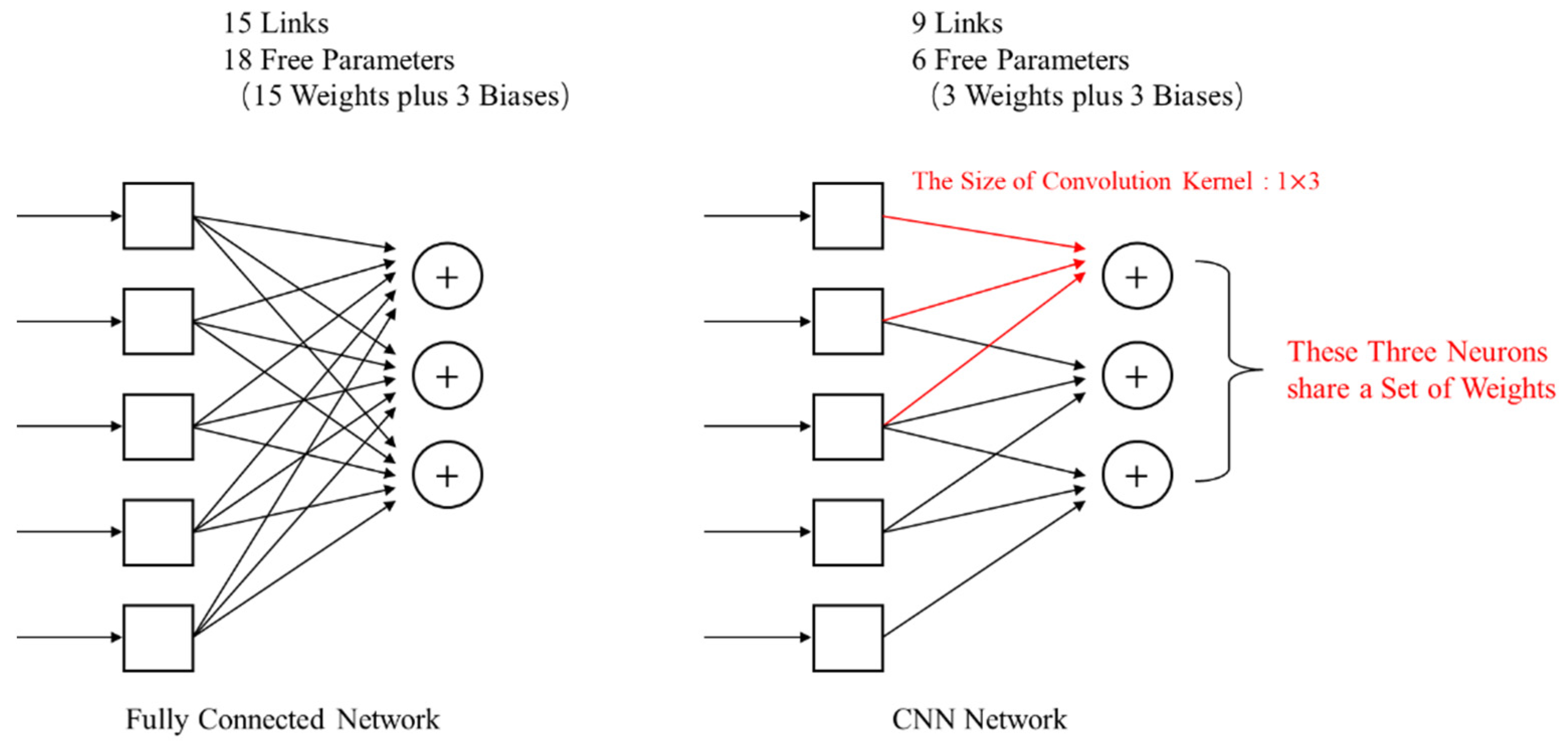
CNN is a model proposed because of the enlightenment of the neural mechanism of the visual system, which can be regarded as an extension of the ordinary neural network [18,35]. Its core idea lies in the local receptive field and weight sharing. As illustrated in Figure 1, a local receptive field is one in which an optic nerve considers only a tiny area of visual input; compared with the full-connection layer of an ordinary neural network, where each neuron in the subsequent layer must be connected to all the nodes in the previous layer [36,37], each node of a specific layer in CNN is only responsible for a specific area of input of the previous layer (such as a 1 $\times$ 3 neighborhood). In this way, the number of weights to be trained will be significantly reduced compared with the full connection, thus reducing the requirement on sample space size; weight sharing implies that all neurons in a hidden layer share a set of weights, which simplifies the network structure by reducing the number of network parameters.

Based on the above analysis, it can be seen that a convolutional neural network requires fewer parameters to train than other fully connected networks, and the network structure is simpler, which can improve work efficiency. Therefore, CNN is selected as the training model in this paper.

2.3. One-Dimensional CNN Model Building

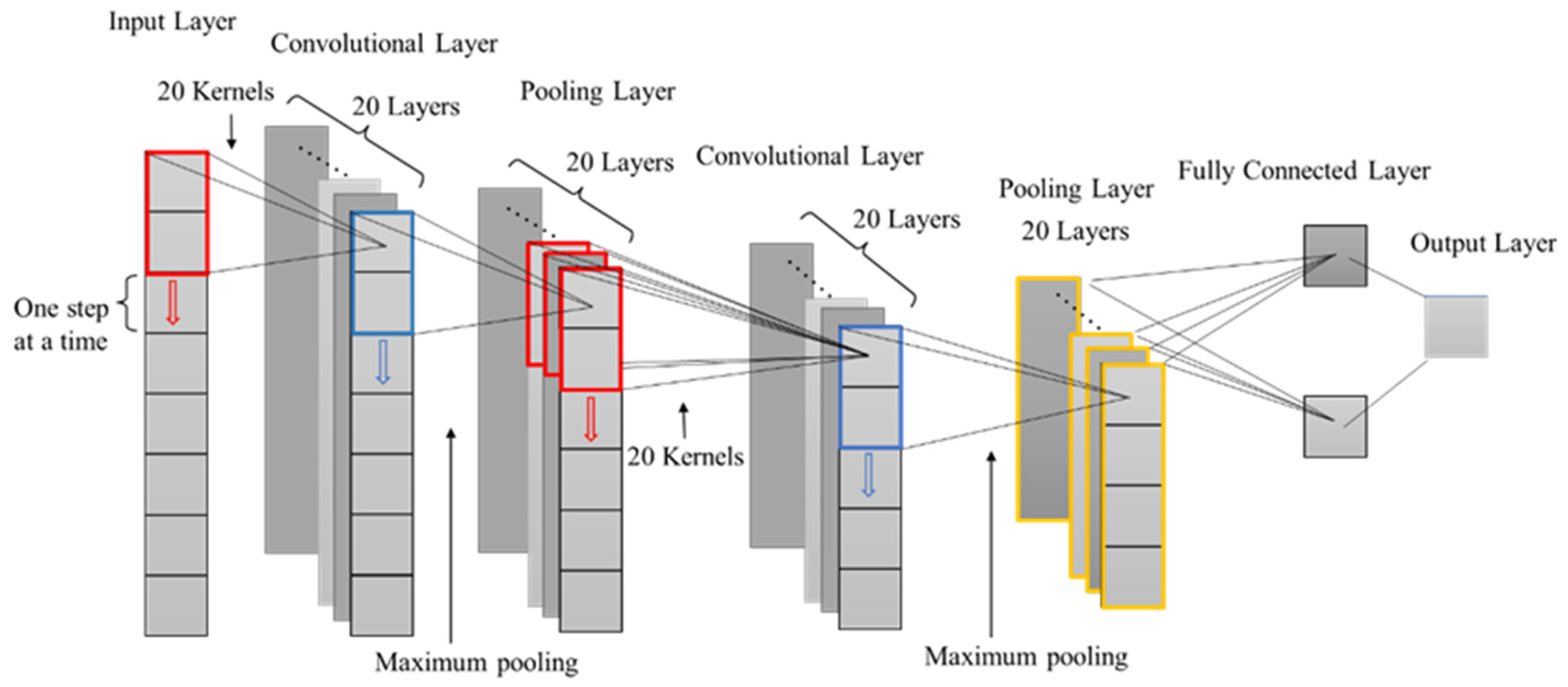
In this experiment, eight kinds of seismic attributes are selected to form one-dimensional data as the input features of samples (the details as shown in

Table 1. Eight seismic attributes.

Serial Number	Seismic Attribute
1	Var
2	Dip
3	Chaos
4	Reflection magnitude
5	Instantaneous phase
6	Instantaneous frequency
7	RMS amplitude
8	Max amplitude

). When the network input is one-dimensional data, a relatively simple one-dimensional CNN is typically chosen for structure selection, as this type of network is frequently utilized in signal processing analysis, speech recognition, and other fields [38]. Since the network takes one-dimensional data as input, its convolution kernel adopts a one-dimensional structure. Convolutional and pooling layers both produce a one-dimensional feature vector as their output.

Three convolutional neural network structures are established in this paper, and the main difference between them is the number of convolution kernels. Only the first network model is introduced in detail here. The basic structure of the first network model is shown in Figure 2. The model takes eight seismic attributes as input and is mainly divided into two structures: the convolution layer and the pooling layer. The convolution kernel size of the convolution layer is 1 × 2, and the number is 20. The convolution kernels move one unit at a time. The pooling mode of the pooling layer is maximum pooling, the pooling window size is 1 × 2. It should be noted that each neuron in the second convolution layer is connected to 1 by 2 neighborhoods in multiple feature maps of the previous layer. Each convolution layer and pooling layer contains 20 maps. The output dimension of the full connection layer is 1 × 2, and the output result is a number (sample label).

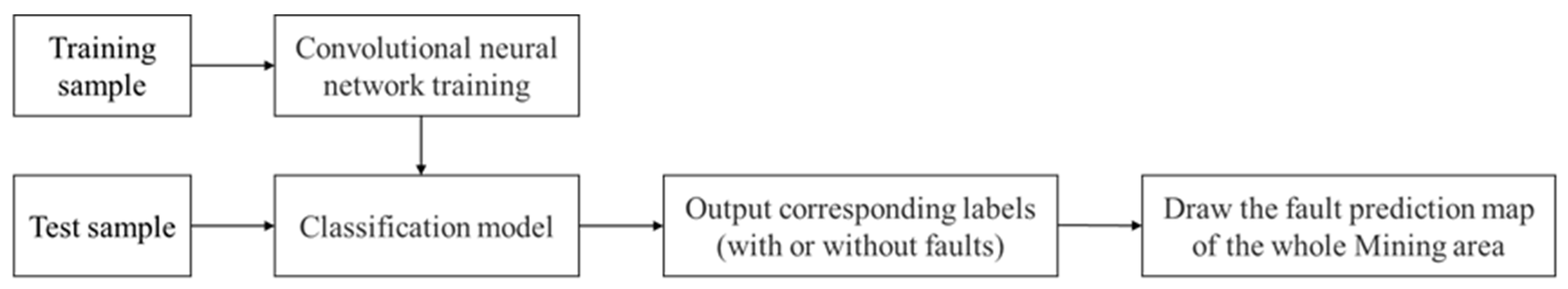
Fault identification based on CNN is regarded as a dichotomous problem. Several seismic attributes are input into the CNN as sample features. The sample points are divided into two categories: non-fault points and fault points, with corresponding sample labels of 0 and 1, respectively. The specific implementation process of fault identification is highlighted in Figure 3. To begin, several known sample points are selected as training samples in actual mining area, and the sample contents include position coordinates and various seismic attributes of these points. The sample label indicates whether there is a fault at the position of sample point. If there is a fault, the label is marked as 1; if there is no fault, the label is marked as 0. Whether there are faults at these sample points is known information. Seismic attributes of known samples as features are input into the convolutional neural network model; then, model training begins. In this process, the weights and biases of connections in the network are constantly adjusted according to the error between actual output value and sample label until they are equal, and then the classification model is generated. After that, the seismic attributes of unknown sample points are input into the classification model. By using the actual output values of model as prediction labels of these samples, we can judge whether there are faults at the positions of these points. In this way, we can get the fault distribution information of the whole mining area. Ultimately, the fault prediction plan for the whole work area is drawn according to the position coordinates of all sample points.

3. Fault Identification Example

Taking a mining area in the east of Yunnan province as an example, seismic data are processed and interpreted by Geoframe software, and the distribution of man-made faults in the mining area is obtained. As shown in Table 1, the mining area attribute data are comprised of eight attributes collected from the seismic data in the mining area. The mining area is depicted in Figure 4, with a total of 159,466 sample points, of which 5800 are known, distributed in the four regions of ABCD.

Table 2. Statistical table of faults in each region.

Regions	A	B	C	D
Number of fault points	216	137	70	128
Number of non-fault points	1896	1711	510	1132
Total number	2112	1848	580	1260
Proportion of fault points	10.23%	7.41%	12.07%	10.16%

summarizes the number and proportion of fault and non-fault points in each region.

3.1. Comparative Experiment of Training Parameter Optimization

The training parameters of CNN mainly include learning rate, batch size, epochs, etc. The learning rate affects the learning speed of the model, while the batch size and epochs affect the training time and test accuracy of the model. The selection of training parameters is a crucial factor in ensuring prediction accuracy. To determine the appropriate training parameters and to improve the classification performance of the model, all known sample points are taken as the training set and test set, while all sample points in the mining area are taken as the prediction set. A network model is established to conduct the comparison experiment for parameter optimization.

In this experiment, the convolutional neural network model is established by MATLABR2019b software. Some initial structural parameters of the model that need to be set are listed in

Table 3. Structural parameters of the model.

Layer	Partial Structural Parameters
Input layer	Input size: 1 $\times$ 8 Eight Seismic Attributes
Convolution layer (C1)	The size of convolution kernel: 1 $\times$ 2 the number of convolution kernel: 20 the activation function: Relu
Pooling layer (S2)	Maximum pooling pooling window size: 1 $\times$ 2 slide step size: 2
Convolution layer (C3)	The size of convolution kernel: 1 $\times$ 2 the number of convolution kernel: 20 the activation function: Relu
Pooling layer (S4)	Maximum pooling pooling window size: 1 $\times$ 2 slide step size: 2
Fully connected layer (F5)	Output size: 1 $\times$ 2
Output layer	The softmax function, with an output value of 0 or 1

.

As depicted in Table 3, the model takes eight seismic attributes as input and is mainly divided into two structures: the convolution layer and the pooling layer. The convolution kernel size of the convolution layer is 1 × 2, and the number is 20. The pooling mode of the pooling layer is maximum pooling, the pooling window size is 1 × 2, and the sliding step size is 2 (i.e., non-overlapping pooling). Relu is used as an activation function. The output dimension of the full connection layer is 1 × 2. The softmax function is employed in the output layer, and the output result is a sample label (0 or 1).

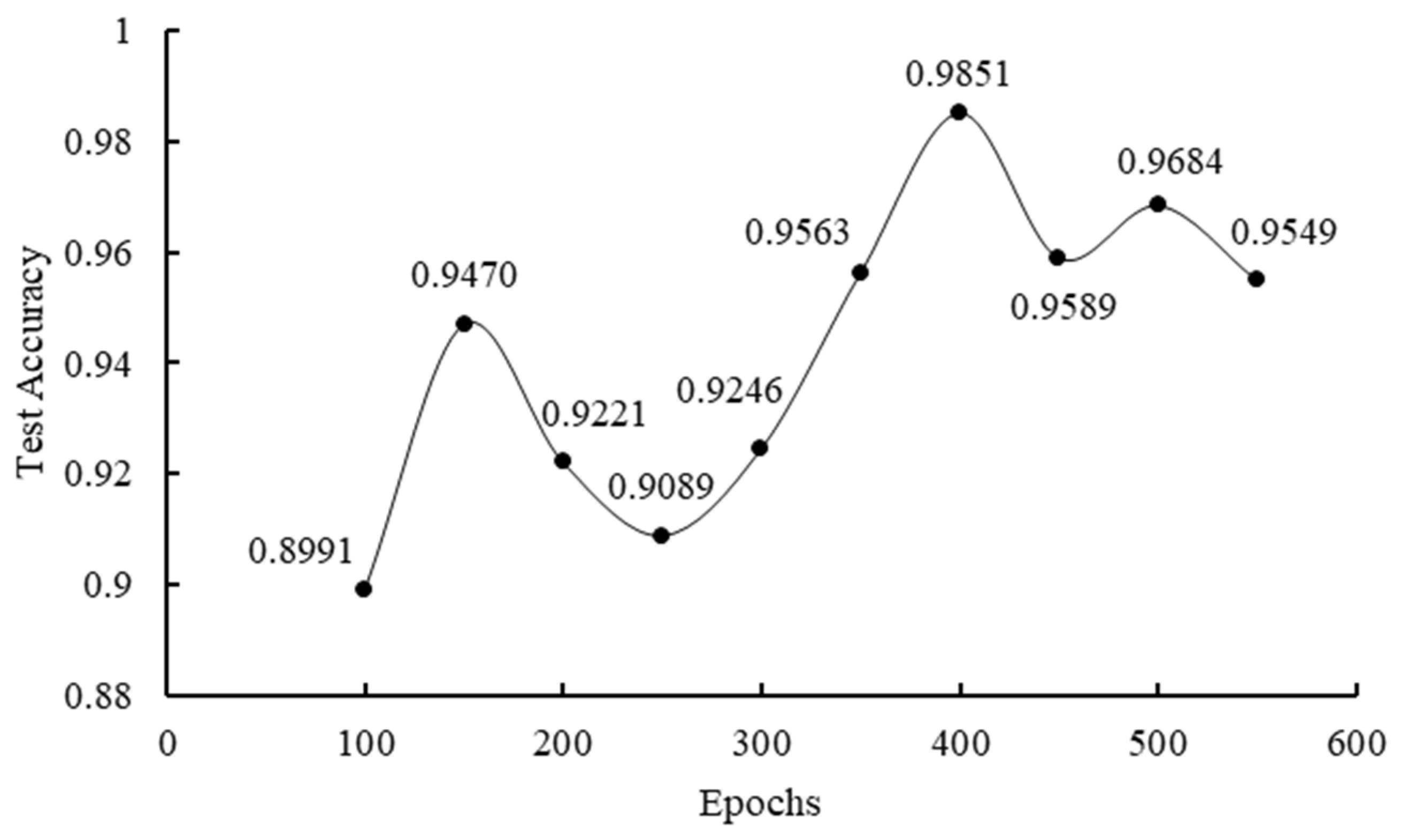
The above model structure is adopted; the learning rate and batch size are fixed: the learning rate is set as 10⁻⁷ and the batch size is set as 100. Epochs are changed several times. Figure 5 and Figure 6 illustrate the test accuracy and training when epochs are set to different values.

As seen in the above figures, as epochs increase from 100, 150, 200, and 250 to 550, the test accuracy will fluctuate within a specific range, peaking when the number of epochs is 400. As the number of training rounds increases, the duration of training time grows proportionately. Considering the two factors of test accuracy and training time, the value of epochs should be set to 400.

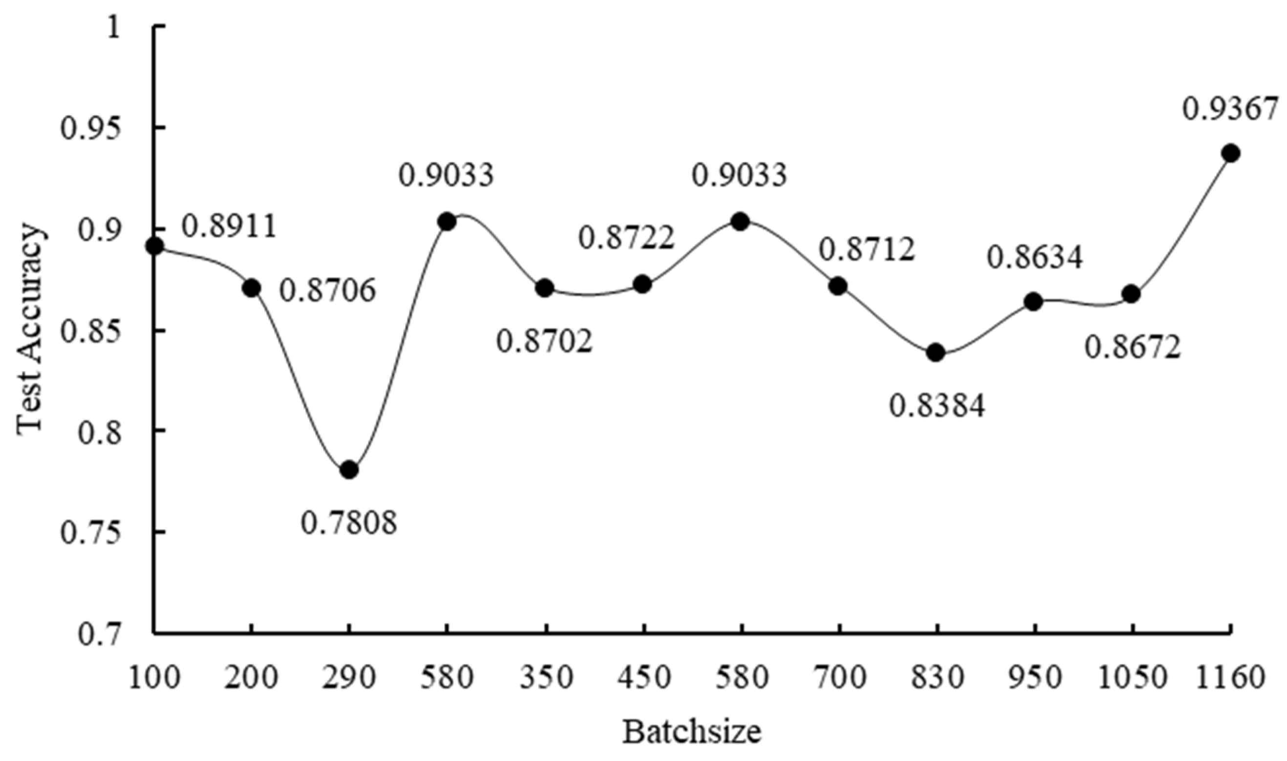
Then, the learning rate and epochs were fixed and set to 10⁻⁷ and 400, respectively, and the batch size was varied several times. When the batch size was varied, the curve illustrating the change in the test accuracy as a function of the batch size is given in Figure 7.

As depicted in Figure 8, when the batch size $\le$ 300, the test accuracy decreases rapidly as the batch size increases. When batch size $\ge$ 300, the test accuracy fluctuates and reaches 0.9367 when the batch size equals 1160. Given that the value of the batch size is too large and will affect the prediction accuracy, the batch size can be set to 200.

Finally, epochs and batch size were fixed and set to 400 and 200, respectively. The value of the learning rate was changed several times. As demonstrated in Figure 8, as the learning rate increases, the test accuracy initially decreases rapidly and then gradually increases. Considering that a low learning rate affects the prediction accuracy, the learning rate is set to 10⁻⁷.

Comparative experiments determined that epochs should be set to 400, the batch size to 200, and the learning rate to 10⁻⁷.

3.2. Comparative Experiment of Model Structure Optimization

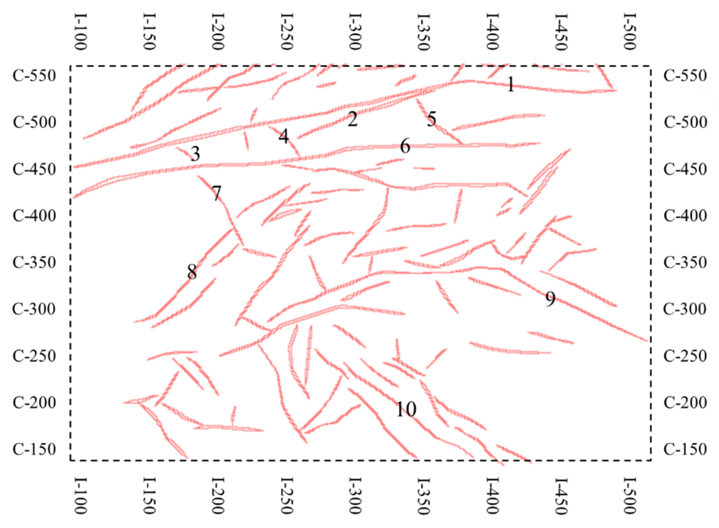
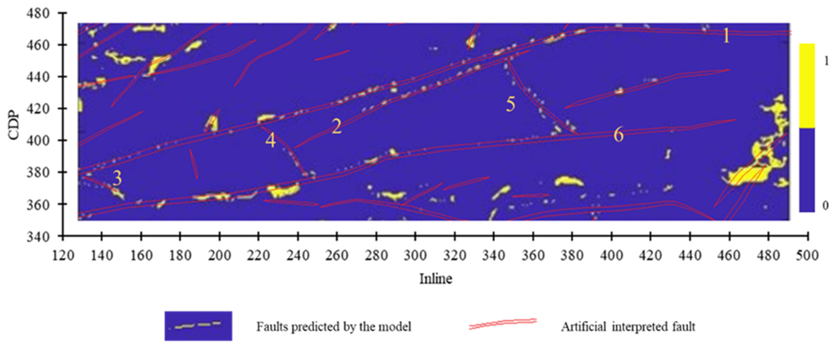
The complexity of the network structure affects the classification ability of the model. If the network is too simple, the training accuracy will reach the expected level, and the model will be incapable of completing the classification task. If the network is overly complicated, over-fitting occurs, and the actual prediction accuracy of the model is extremely low. To choose an appropriate network structure and improve prediction performance, all known sample points served as the training set and test set, while all sample points inside the mining area served as the prediction set. Three models were established, and model parameters are summarized in

Table 4. Structural parameters of Model 1.

Layer	Partial Structural Parameters
Input layer	Input size: 1 $\times$ 8 Eight Seismic Attributes
Convolution layer (C1)	The size of convolution kernel: 1 $\times$ 2 the number of convolution kernel: 20 the activation function: Relu
Pooling layer (S2)	Maximum pooling pooling window size: 1 $\times$ 2 slide step size: 2
Convolution layer (C3)	The size of convolution kernel: 1 $\times$ 2 the number of convolution kernel: 20 the activation function: Relu
Pooling layer (S4)	Maximum pooling pooling window size: 1 $\times$ 2 slide step size: 2
Fully connected layer (F5)	Output size: 1 $\times$ 2
Output layer	The softmax function, with an output value of 0 or 1

,

Table 5. Structural parameters of Model 2.

Layer	Partial Structural Parameters
Input layer	Input size: 1 $\times$ 8 Eight Seismic Attributes
Convolution layer (C1)	The size of convolution kernel: 1 $\times$ 2 the number of convolution kernel: 10 the activation function: Relu
Pooling layer (S2)	Maximum pooling pooling window size: 1 $\times$ 2 slide step size: 1
Convolution layer (C3)	The size of convolution kernel: 1 $\times$ 2 the number of convolution kernel: 10 the activation function: Relu
Pooling layer (S4)	Maximum pooling pooling window size: 1 $\times$ 2 slide step size: 1
Fully connected layer (F5)	Output size: 1 $\times$ 2
Output layer	The softmax function, with an output value of 0 or 1

and

Table 6. Structural parameters of Model 3.

Layer	Partial Structural Parameters
Input layer	Input size: 1 $\times$ 8 Eight Seismic Attributes
Convolution layer (C1)	The size of convolution kernel: 1 $\times$ 2 the number of convolution kernel: 4 the activation function: Relu
Pooling layer (S2)	Maximum pooling pooling window size: 1 $\times$ 2 slide step size: 1
Convolution layer (C3)	The size of convolution kernel: 1 $\times$ 2 the number of convolution kernel: 4 the activation function: Relu
Pooling layer (S4)	Maximum pooling pooling window size: 1 $\times$ 2 slide step size: 1
Fully connected layer (F5)	Output size: 1 $\times$ 2
Output layer	The softmax function, with an output value of 0 or 1

. Model 1 was identical to the model used in the parameter optimization experiment. The Model 1 network structure was the most complex, while the Model 3 was the simplest. Ten faults in the mining area were selected for comparative analysis of the prediction effect, and specific fault selection is shown in Figure 9.

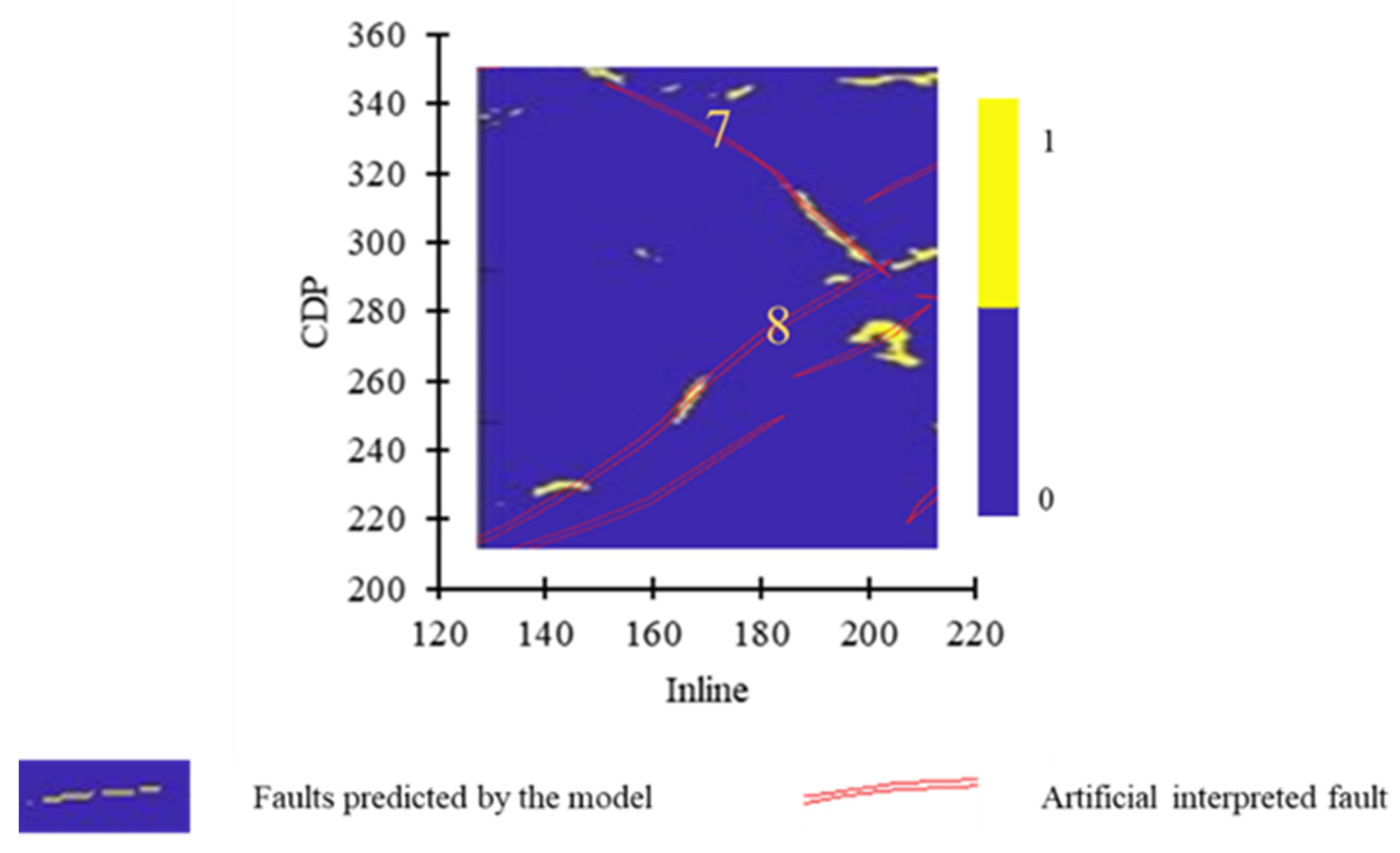
Ten faults in Figure 9 are classified based on their fault extension length. Big faults are Fault 1, Fault 6, and Fault 9; secondary faults are Fault 2, Fault 7, Fault 8, and Fault 10; small faults are Fault 3, Fault 4, and Fault 5. Fault 9 and Fault 10 are located in small-fault concentrated areas where the geological condition is complex. Three models are conducted to predict the 10 faults listed above.

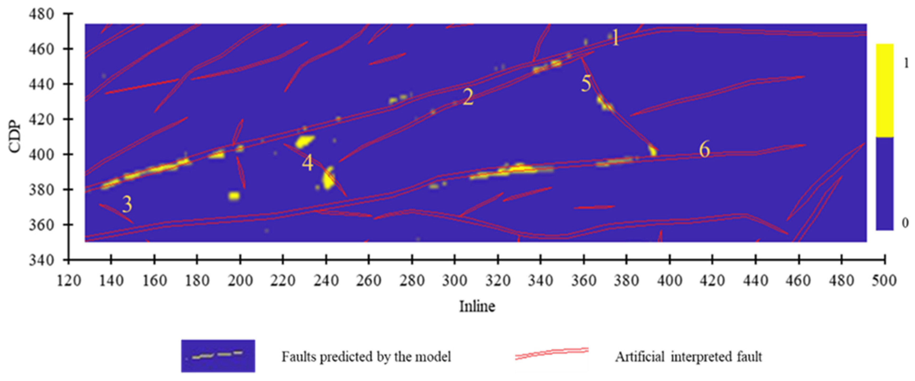
As illustrated in Figure 10, the predicting result of Model 1 only contains prediction points for Fault 1, Fault 3, and Fault 6. Prediction continuity is weak for Fault 1, the posterior segment of Fault 6 is missing, and the prediction effect for Fault 3 is excellent. Faults 7–10 were not predicted.

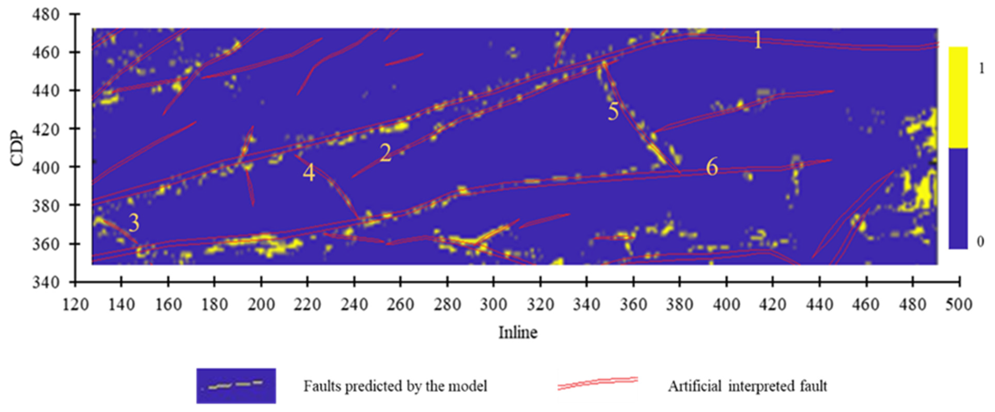
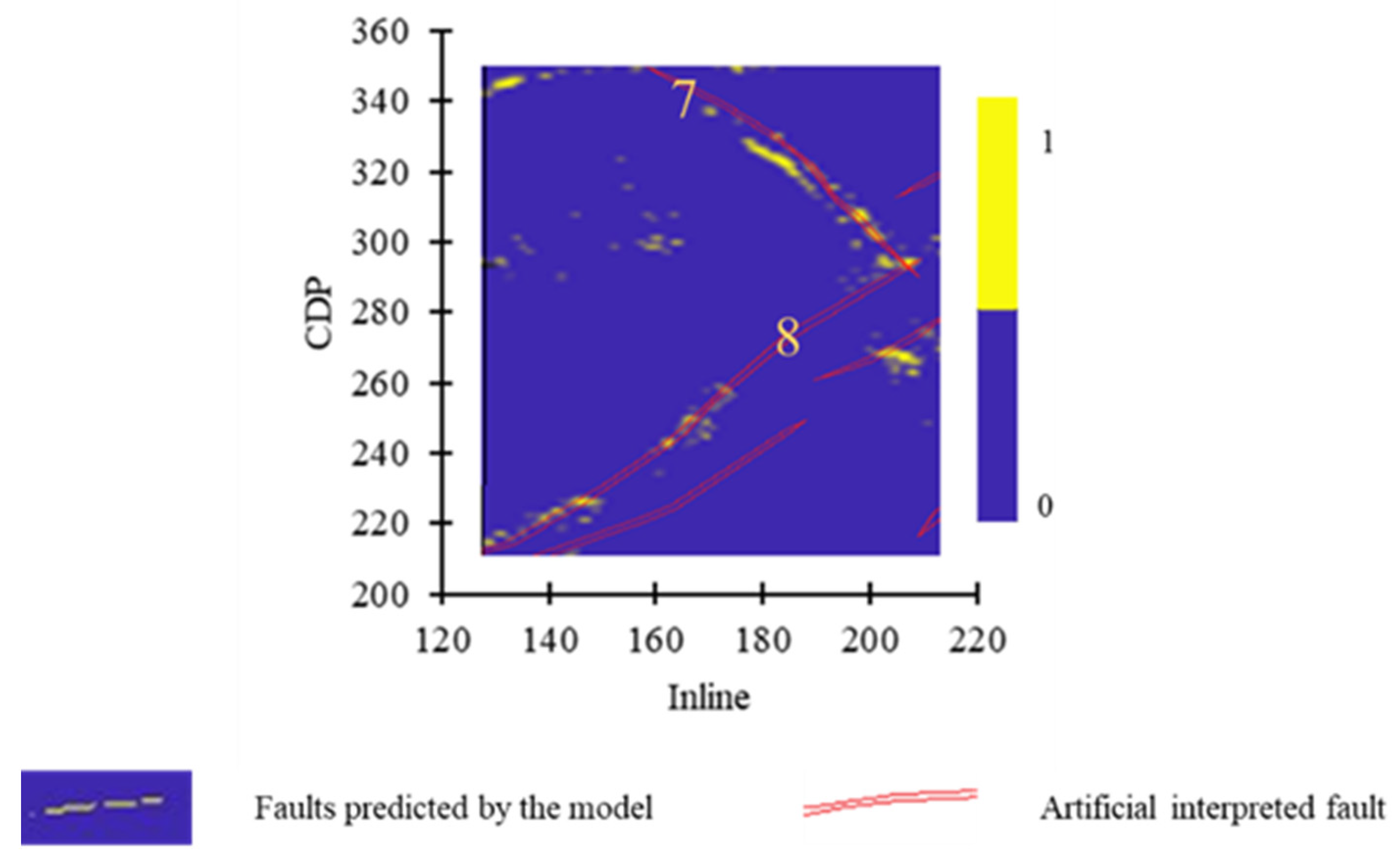
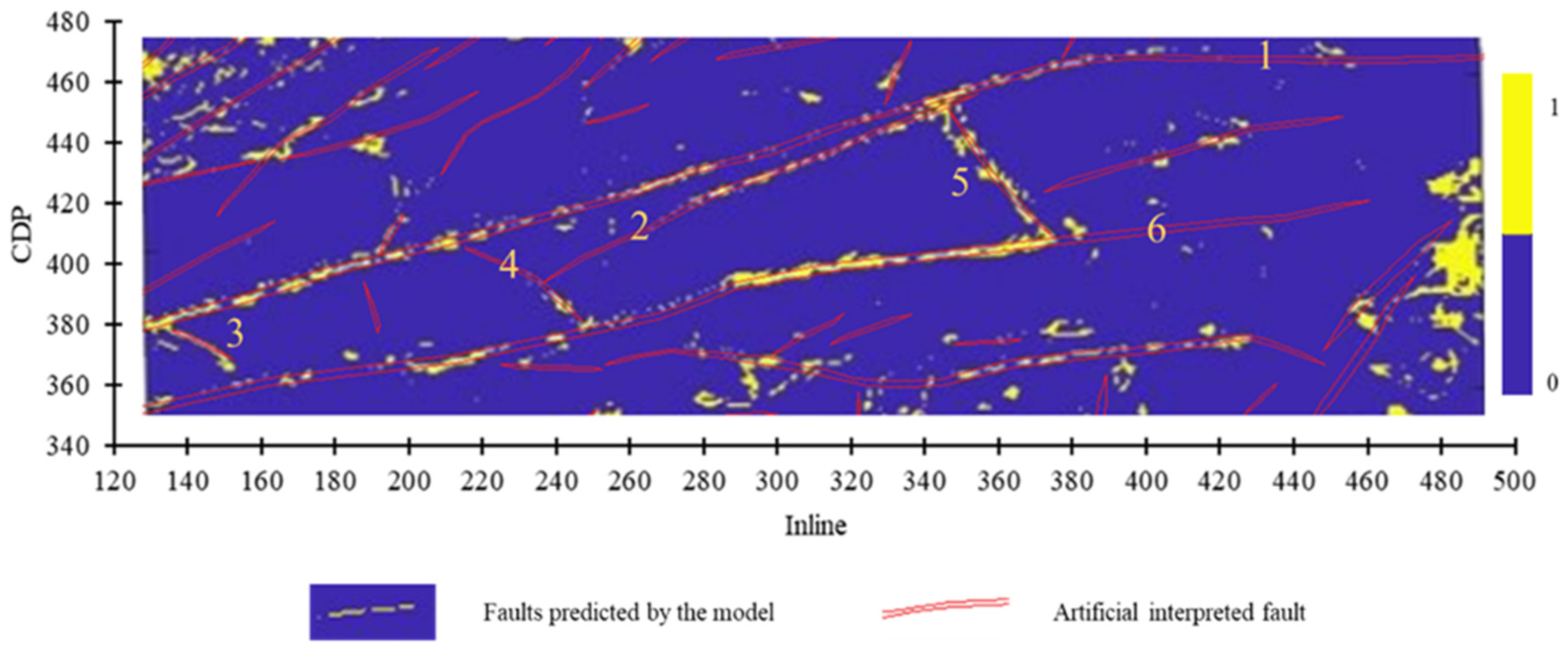
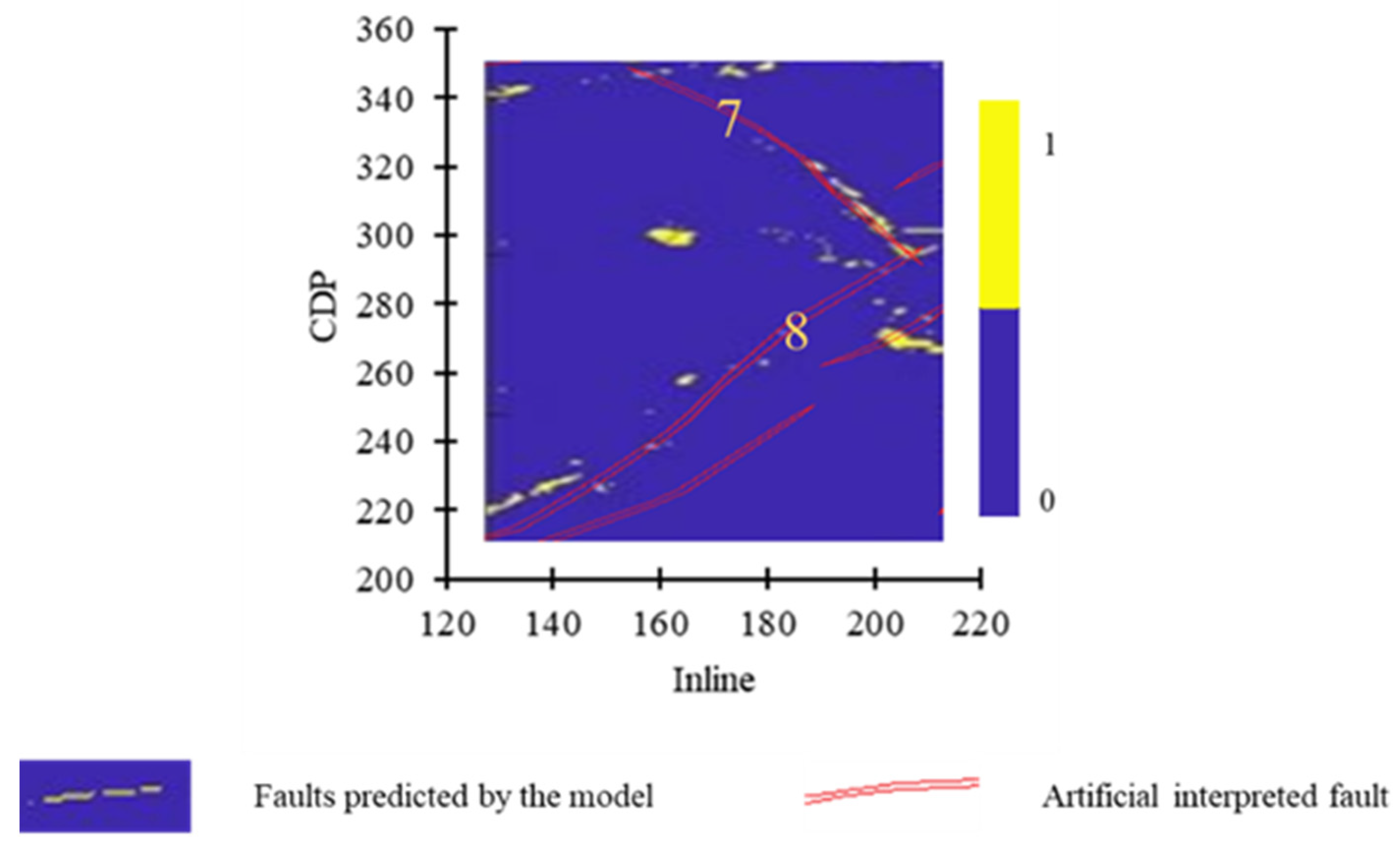
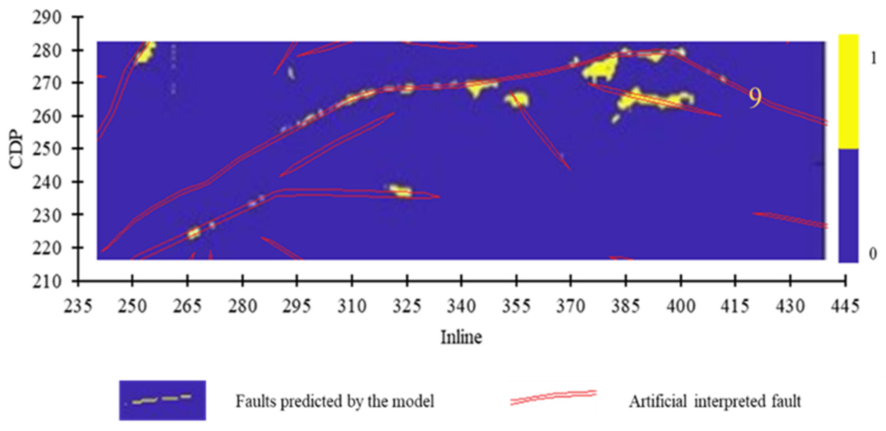
The prediction result of Model 2 is depicted in Figure 11 and Figure 12. The prediction effect of Model 2 on Faults 1–8 is excellent, with only a small portion missing in the rear segment of Fault 1, and the continuity of the right end of Fault 6 is slightly worse than its left end. Faults 9 and 10 remain unknown.

As shown in Figure 13, Model 3 can only show Fault 1 and Fault 6, and other faults cannot be predicted.

By comparing and analyzing the prediction impacts of the three models, it is discovered that the fault identification effect of Model 2 is much better than that of Model 1 and Model 3, and the continuity is excellent. Model 1 has a few faults, but the prediction points are scattered, and the continuity needs improvement. The continuity of Model 3’s fault prediction results is more consistent than that of Model 1, yet Model 3 could predict too few faults. Therefore, it is speculated that the network structure of Model 1 is too complex for this dataset, and there may be an over-fitting effect lowing the prediction level. In addition, the structure of Model 3 is oversimplified, resulting in a poor prediction effect. Under the same dataset, Model 2 is more suitable for fault prediction.

3.3. Comparative Experiment of Zonal Training Model

All known sample points in the mining area are distributed in regions, including Region A, Region B, Region C, and Region D (Figure 4). In Region A, large faults predominate, but in Region B, small faults are relatively developed. While both Region C and Region D have a comparable number of large and small faults, the difference lies in that the small faults in Region C are concentrated between the two large faults, whereas the small faults in Region D are distributed outside the two large faults. Due to the fault distribution varying among regions, the prediction results would change by employing known sample points from different regions as training sets. To explore the influence of different training sets on the model prediction effect, the known sample points in four regions are used to create training and test sets (Model 2 in the comparative experiment was used as the model structure). Finally, the entire mining area was predicted, and the prediction effect on 10 faults exhibited in Figure 9 was compared and analyzed.

The four regions as training sets to predict faults are described below.

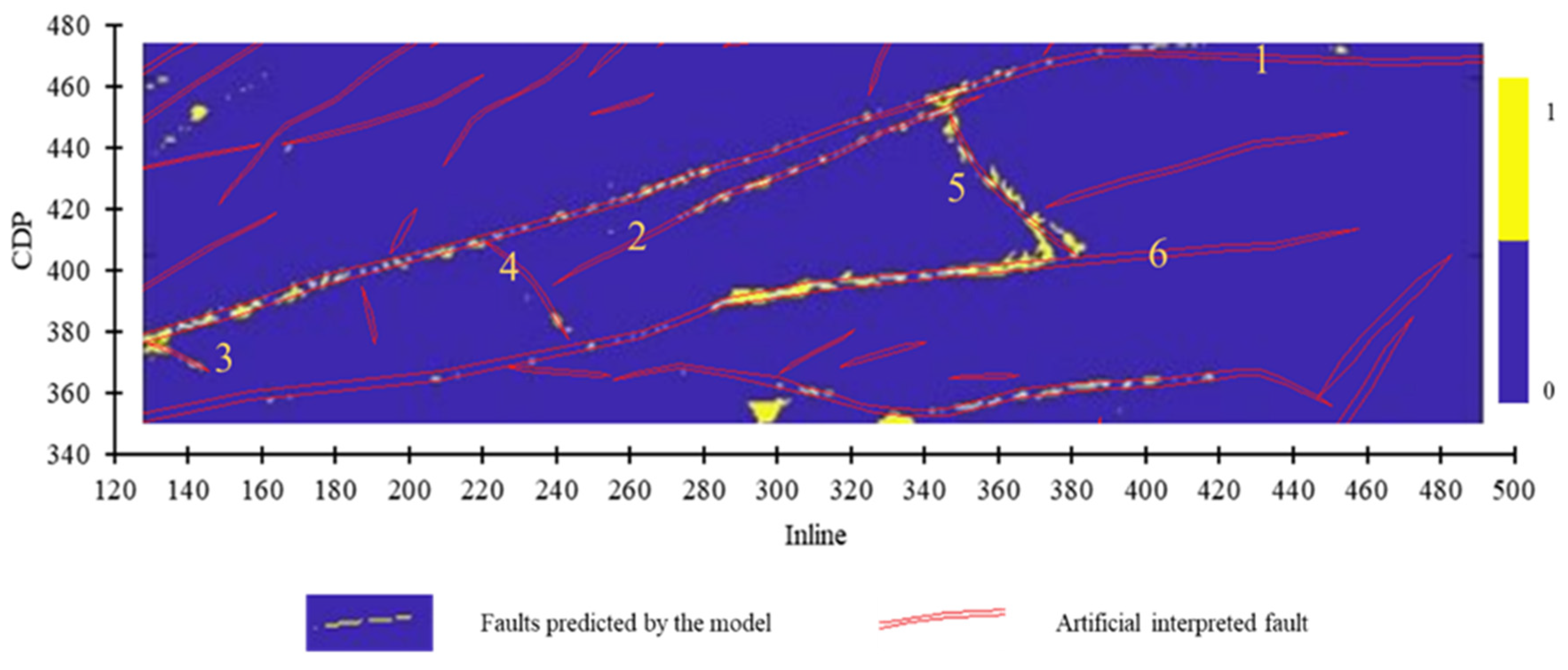
As shown in Figure 14, Figure 15 and Figure 16, Region A can accurately predict Faults 1–8, but Fault 9 and Fault 10 exhibit poor continuity of prediction findings. It is discovered that the model using Region A as the training set has a generally good prediction effect. The two large faults in the mining area, Fault 1 and Fault 6, are prominently visible. Fault 3, Fault 4, and Fault 5 as small faults can also be predicted.

Only small faults, such as Faults 3–5, and a large fault, Fault 10, can be predicted using Region B as the training set. As Figure 17 shows, the prediction result on Fault 9 by Region B is more precise than that by Region A.

Figure 18, Figure 19 and Figure 20 show that Region C has a more favorable prediction effect on Faults 1–5. The left segment of Fault 6 has a weak continuity of prediction results, the center segment has a strong continuity, and the right segment is missing. Region C is capable of predicting Fault 9 and Fault 10, and the continuity of the predicting result on Fault 9 is greater than that of Region B.

The fault prediction result by Region D is displayed in Figure 21 and Figure 22. Fault 1 to Fault 8 can be predicted, but the continuity of predicting results is not as good as Region A and Region C.

The model test accuracy under various training sets is displayed in

Table 7. Model test accuracy under different training sets.

Training Set	Test Accuracy
Region A	85.26%
Region B	87.59%
Region C	88.28%
Region D	87.00%

. After a comprehensive analysis of each region’s prediction results and test accuracy, it can be concluded that the overall prediction results of Region A and Region C are superior and more continuous than the other two regions. While Region B and Region D have higher test accuracy than that Region A, the actual prediction effect is general, indicating that the training set with high test accuracy may not always predict the faults well. Therefore, it is necessary to select the training set to predict faults by considering both accuracy and actual prediction effect. Regardless of the model used or the region selected as the training set, Faults 9–10 have lower predictive results than Faults 1–8. As the regional geological situation involving these two faults become relatively complicated, the prediction complexity increases, necessitating either optimization of the model structure for this region or an increase in the number of training samples to improve the prediction accuracy.

When the results of model interpretation and manual interpretation are compared, it is found that, under the premise of correctly choosing model parameters and training set, the difference between the two is not very huge, and the distribution of faults is consistent, with only minor differences in some faults. In addition, combining the artificial interpretation fault with the predictive method of CNN models can improve interpretation efficiency and save manpower and time.

4. Conclusions

In this paper, eight different types of seismic attributes were employed as feature inputs to the CNN model, and a training set was created based on the actual data of a mining area in eastern Yunnan province to predict the faults. To optimize the selection of the model parameters and create the training set, an optimization experiment for the model training parameters was conducted. A comparison experiment for the model structural parameters and training set were set up. Ten faults in the area were selected to analyze the prediction result, and the following conclusions were obtained:

• Training parameters have a significant impact on the model’s training time and test accuracy. Through training parameters optimization experiments, it is discovered that epochs, batch size, and learning rate all influence the testing accuracy of the model. Additionally, the training of the model takes longer as the epochs increase. It is necessary to determine the optimal combination of training parameters for a specific network structure by repeatedly adjusting parameters, thereby improving the prediction accuracy and reducing the training time of the model.
• The model’s structural parameters have a great impact on the actual prediction result. Comparing the prediction results of the three models (Table 4, Table 5 and Table 6) on faults reveals that the actual prediction effects of CNN models with different network structures on faults are considerably varied for the same training set. When defining the model’s structural parameters, it is vital to select an appropriate network complexity according to the characteristics of the dataset. If the network is either too complex or too simple, the actual prediction accuracy of faults will be reduced.
• When creating the training set by area, the prediction effect and the test accuracy of the model are different. The more representative the fault distribution in the region is, the more abundant the training set samples are, and the better the prediction effect of the model will be. Since the actual prediction effect of a model with high test accuracy may be suboptimal, it is vital to comprehensively examine both accuracy and actual prediction effect when selecting a model to predict faults.
• On the premise of appropriately selecting model parameters and training sets, CNN’s interpretation results of faults are in good agreement with manual interpretation results. Major faults have a uniform distribution pattern, with variations occurring primarily in individual locations. The time taken is considerably shortened compared to manual interpretation, and the test accuracy is over 85%. It demonstrates that this method can effectively improve the accuracy and efficiency of fault interpretation with certain feasibility.
• In this paper, the limitation of the automatic fault recognition model based on CNN is that because of the one-dimensional network structure the model’s capacity to input feature information is smaller than that of a two-dimensional structure, resulting in the loss of some fault attribute information.

The results obtained in this experiment have been applied to roadway layout in the Eastern Yunnan Province Mining Company of China Huaneng Group. According to the design of the working face in the mining area, it is estimated that two 60 m faults will lead to the abandonment, repair, and adjustment of about 200 m of roadway in the case that the large structure has not been proved. Referring to the comprehensive investment of RMB 100,000/meter in the roadway in the adjacent mining area, this study is expected to save the economic investment of RMB 20 million for the enterprise.

5. Patent

The extraction method and system of training set for machine learning model of seismic fault (2020106379337).

References

- Cunningham, J.E.; Cardozo, N.; Townsend, C.; Callow, R.H.T. The impact of seismic interpretation methods on the analysis of faults: A case study from the Snøhvit field, Barents Sea. Solid Earth Discuss. 2021, 12, 1–48. [Google Scholar] [CrossRef]
- Alcalde, J.; Bond, C.E.; Johnson, G.; Robert, W.H.; Butler, M.; Cooper, A.; Ellis, J.F. The importance of structural model availability on seismic interpretation. J. Struct. Geol. 2017, 97, 161–171. [Google Scholar] [CrossRef] [Green Version]
- Alcalde, J.; Bond, C.E.; Johnson, G.; Ellis, J.F.; Butler, R.W.H. Impact of seismic image quality on fault interpretation uncertainty. GSA Today 2017, 27, 4–10. [Google Scholar] [CrossRef]
- Physics—Geophysics. Studies Conducted at School of Electrical and Computer Engineering on Geophysics Recently Reported (Semi-automatic Fault/fracture Interpretation Based on Seismic Geometry Analysis). J. Phys. Res. 2019.
- Godefroy, G.; Caumon, G.; Laurent, G.; Bonneau, F. Structural Interpretation of Sparse Fault Data Using Graph Theory and Geological Rules. Math. Geosci. 2019, 51, 1091–1107. [Google Scholar] [CrossRef] [Green Version]
- Faleide, T.S.; Braathen, A.; Lecomte, I.; Mulrooney, M.J.; Midtkandal, I.; Bugge, A.J.; Planke, S. Impacts of seismic resolution on fault interpretation: Insights from seismic modelling. Tectonophysics 2021, 816, 229008. [Google Scholar] [CrossRef]
- Jingbin, C.; Zhonghong, W.; Ping, C.; Quanhu, L.; Chen, X. The application of seismic attribute analysis technique in coal field exploration. Interpretation 2016, 4, SB13–SB21. [Google Scholar] [CrossRef] [Green Version]
- Oumarou, S.; Mabrouk, D.; Tabod, T.C.; Marcel, J.; Ngos, S., III; Essi, J.M.A.; Kamguia, J. Seismic attributes in reservoir characterization: An overview. Arab. J. Geosci. 2021, 14, 1–15. [Google Scholar] [CrossRef]
- Xu, T. Reservoir Prediction Method by Seismic Attribute Based on Reservoir Classification. J. Pet. Min. Eng. 2020, 3. [Google Scholar]
- Wu, B.; Kong, J.; Dong, S. Seismic attribute method for concealed collapse column identification in coal fields. Acta Geod. Geophys. 2020, 55, 11–21. [Google Scholar] [CrossRef]
- Zhang, B.; Liu, Y.; Pelissier, M.; Hemstra, N. Semiautomated fault interpretation based on seismic attributes. Interpretation 2014, 2, SA11–SA19. [Google Scholar] [CrossRef]
- Li, K.; Xi, Y.; Su, Z.; Zhu, J.; Wang, B. Research on reservoir lithology prediction method based on convolutional recurrent neural network. Comput. Electr. Eng. 2021, 95, 107404. [Google Scholar] [CrossRef]
- Odoh, B.I.; Ilechukwu, J.N.; Okoli, N.I. The Use of Seismic Attributes to Enhance Fault Interpretation of OT Field, Niger Delta. Int. J. Geosci. 2014, 5, 826–834. [Google Scholar] [CrossRef] [Green Version]
- Liu, W.J.; Liu, W.M.; Zhao, S.N.; Chen, Q. RGB Fusion of Seismic Attributes and its Application on Small Structure Interpretation in Coalmine. Appl. Mech. Mater. 2014, 651, 1245–1248. [Google Scholar] [CrossRef]
- Sun, Z.; Peng, S.; Zou, G. Automatic recognition of small seismic faults based on SVM algorithm. J. China Coal Soc. 2017, 11, 2945–2952. [Google Scholar]
- Kim, M.; Yu, J.; Kang, N.K.; Kim, B.Y. Improved Workflow for Fault Detection and Extraction Using Seismic Attributes and Orientation Clustering. Appl. Sci. 2021, 11, 8734. [Google Scholar] [CrossRef]
- Lecun, Y.; Bengio, Y.; Hinton, G. Deep learning. Nature 2015, 521, 436. [Google Scholar] [CrossRef]
- Chen, L.C.; Papandreou, G.; Kokkinos, I.; Murphy, K.; Yuille, A.L. DeepLab: Semantic Image Segmentation with Deep Convolutional Nets, Atrous Convolution, and Fully Connected CRFs. IEEE Trans. Pattern Anal. Mach. Intell. 2018, 40, 834–848. [Google Scholar] [CrossRef] [Green Version]
- LeCun, Y.; Boser, B.; Denker, J.S.; Henderson, D.; Howard, R.E.; Hubbard, W.; Jackel, L.D. Backpropagation applied to handwritten zip code recognition. Neural Comput. 1989, 1, 541–551. [Google Scholar] [CrossRef]
- LeCun, Y.; Bottou, L.; Bengio, Y.; Haffner, P. Gradient-based learning applied to document recognition. Proc. IEEE 1998, 86, 2278–2324. [Google Scholar] [CrossRef] [Green Version]
- Gupta, A.; Narwaria, R.P.; Singh, M. Review on Deep Learning Handwritten Digit Recognition using Convolutional Neural Network. Int. J. Recent Technol. Eng. 2021, 9, 245–247. [Google Scholar] [CrossRef]
- Krizhevsky, A.; Sutskever, I.; Hinton, G.E. ImageNet classification with deep convolutional neural networks. In Proceedings of the Advances in Neural Information Processing Systems 25, Lake Tahoe, NV, USA, 3–6 December 2012; Curran Associates: Red Hook, NY, USA, 2012; pp. 1097–1105. [Google Scholar]
- Umer, S.; Mondal, R.; Pandey, H.M.; Rout, R.K. Deep features based convolutional neural network model for text and non-text region segmentation from document images. Appl. Soft Comput. J. 2021, 113, 107917. [Google Scholar] [CrossRef]
- Yue, X.; Lyu, B.; Li, H.; Meng, L.; Furumoto, K. Real-time medicine packet recognition system in dispensing medicines for the elderly. Meas. Sens. 2021, 18, 100072. [Google Scholar] [CrossRef]
- Liu, W.; Sun, H.; Jia, Z.; Yu, X. Surface mounted devices classification using a mixture network of DCNN and DFCN. Neurocomputing 2021, 465, 428–436. [Google Scholar] [CrossRef]
- Rani, R.; Singh, G.B.; Sharma, N.; Kakkar, D. Identification of Tomato Leaf Diseases Using Deep Convolutional Neural Networks. Int. J. Agric. Environ. Inf. Syst. 2021, 12, 1–22. [Google Scholar]
- Zhuang, J.; Li, X.; Bagavathiannan, M.; Jin, X.; Yang, J.; Meng, W.; Li, T.; Li, L.; Wang, Y.; Chen, Y.; et al. Evaluation of different deep convolutional neural networks for detection of broadleaf weed seedlings in wheat. Pest Manag. Sci. 2021, 78, 521–529. [Google Scholar] [CrossRef]
- Dokur, Z.; Olmez, T. Classification of motor imagery electroencephalogram signals by using a divergence based convolutional neural network. Appl. Soft Comput. J. 2021, 113, 107881. [Google Scholar] [CrossRef]
- Zhou, D.-X. Deep distributed convolutional neural networks: Universality. Anal. Appl. 2018, 16, 895–919. [Google Scholar] [CrossRef]
- Li, Z.; Liu, F.; Yang, W.; Peng, S.; Zhou, J. A Survey of Convolutional Neural Networks: Analysis, Applications, and Prospects. In IEEE Transactions on Neural Networks and Learning Systems; Institute of Electrical and Electronics Engineers (IEEE): Piscataway, NJ, USA, 2021. [Google Scholar]
- Zhang, Z.; Yan, Z.; Gu, H. Automatic fault recognition based on residual network and migration learning. Pet. Geophys. Explor. 2020, 55, 950–956. [Google Scholar]
- Wu, X.M.; Hale, D. Automatically interpreting all faults, unconformities, and horizons from 3D seismic images. Interpret. A J. Subsurf. Charact. 2016, 4, T227–T237. [Google Scholar] [CrossRef] [Green Version]
- Guo, B.; Li, L.; Luo, Y. A new method for automatic seismic fault detection using convolutional neural network. SEG Tech. Program Expand. Abstr. 2018, 1951–1955. [Google Scholar]
- Zou, G.; Ren, K.; Sun, Z.; Peng, S.; Tang, Y. Fault interpretation using a support vector machine: A study based on 3D seismic mapping of the Zhaozhuang coal mine in the Qinshui Basin, China. J. Appl. Geophys. 2019, 171, 103870. [Google Scholar] [CrossRef]
- Szegedy, C.; Liu, W.; Jia, Y.; Sermanet, P.; Reed, S.; Anguelov, D.; Erhan, D.; Vanhoucke, V.; Rabinovich, A. Going Deeper with Convolutions. IEEE Comput. Soc. 2014, 1–9. [Google Scholar]
- Basheer, I.A.; Hajmeer, M. Artificial neural networks: Fundamentals, computing, design, and application. J. Microbiol. Methods 2000, 43, 3–31. [Google Scholar] [CrossRef]
- Jin, W.; Li, Z.J.; Wei, L.S.; Zhen, H. The Improvements of BP Neural Network Learning Algorithm. In Proceedings of the 5th International Conference on Signal Processings, Beijing, China, 21–25 August 2000; Volume III, pp. 263–265. [Google Scholar]
- Olkhovskiy, M.; Müllerová, E.; Martínek, P. Impulse signals classification using one dimensional convolutional neural network. J. Electr. Eng. 2020, 71, 397–405. [Google Scholar] [CrossRef]
Figure 1.
Structural comparison between CNN and fully connected networks (take the simple structure as an example).
Figure 2.
Basic structure of the first CNN model.
Figure 3.
The flowchart of fault identification by CNN.
Figure 4.
The plan of the mining area.
Figure 5.
The relationship between test accuracy and epochs.
Figure 6.
The relationship between training time and epochs.
Figure 7.
The relationship between test accuracy and batch size.
Figure 8.
The relationship between test accuracy and learning rate.
Figure 9.
Ten faults in the mining area were selected for comparative experiment.
Figure 10.
Prediction result of Model 1.
Figure 11.
Results of Faults 1–6 predicted by Model 2.
Figure 12.
Prediction result of Fault 7 and Fault 8 by Model 2.
Figure 13.
Result of Faults 1–6 predicted by Model 3.
Figure 14.
The prediction result of Faults 1–6 by Region A as training set.
Figure 15.
The prediction result of Faults 7–8 by Region A as training set.
Figure 16.
The prediction result of Faults 9–10 by Region A as a training set.
Figure 17.
The prediction result of Fault 9 by Region B as a training set.
Figure 18.
The prediction result of Faults 1–6 by Region C as training set.
Figure 19.
The prediction result of Fault 9 by Region C as training set.
Figure 20.
The prediction result of Fault 10 by Region C as training set.
Figure 21.
The prediction result of Faults 1–6 by Region D as training set.
Figure 22.
The prediction result of Faults 7–8 by Region D as training set.