Fluid–Structure Coupling Analysis of the Stationary Structures of a Prototype Pump Turbine during Load Rejection

Abstract

During the load rejection transient process of the prototype pump turbine units, the pressure fluctuations of the entire flow passage change drastically due to the rapid closing of guide vanes. The extremely unsteady pressure distribution in the flow domains including the crown chamber and the band chamber may cause a strong vibration on the stationary structures of the unit and result in large dynamic stress on the head cover, stay ring and bottom ring. In this paper, the numerical fluid dynamic analysis of the entire flow passage of a reversible prototype pump turbine during load rejection was performed. The flow characteristics in the runner passage, crown chamber, band chamber, seal labyrinths and balance tubes are analysed. The corresponding unsteady flow-induced dynamic behaviour of the head cover, stay vanes and bottom ring was investigated in detail. The analysed results show that the total deformation of the inner edge of the head cover closed to the main shaft is larger than that of other stationary structures of the unit during the load rejection. The maximum stress of the stay ring is larger than that of the head cover and the bottom ring and the maximum equivalent stress is located at the fillet of the stay vane trailing edge. The fluid–structure coupling calculation method and the analysed results can provide guidance for the design of stationary components of hydraulic machinery such as pump turbines, Francis turbines and centrifugal pumps with different heads.

1. Introduction

With the gradual increase in power demand in recent decades, the capacity of traditional power generation such as thermal power and nuclear power has been increasing and the peak-to-valley difference of the power grid has been expanding, which has put forward higher requirements on the regulation capability and flexibility of the grid. As an important source of clean and renewable energy, hydropower has increasingly been developed for power generation worldwide because of its flexible features such as fast start/stop and load adjustment. Hydropower has indeed improved the power grid’s ability to resist fluctuations in power demand and has gradually occupied an important share of the grid load. The hydraulic pumped storage power plant (HPSPP) mainly consists of an upstream reservoir, water diversion pipelines, a pumped storage unit and a downstream reservoir. The pump turbine (PT) is the core working equipment of an HPSPP, which can freely choose the direction of energy conversion. When the unit operates under the turbine condition, water flow enters the unit from the spiral case and generates power through the runner. When the unit operates under the pump condition, the flow direction is the opposite and the flow from the draft tube is pumped upstream by the rotating runner. The HPSPP can flexibly select operating conditions according to the demand of the power grid and has functions of peak shaving, valley shaving, frequency regulation, emergency reserve and optimal power supply, which has been vigorously developed and widely used.

The high water head of HPSPP will lead to high pressure excitation on the pump turbine unit and may cause a series of safety problems such as unexpected severe vibration and even fatigue failure on the PT structures. Several cases of unit failure or damage were reported in studies [1,2,3,4]. The main reasons for the failure and damage revealed in the reports include the drastic change of hydraulic characteristics under certain operating conditions, abnormal vibration of the unit caused by unreasonable design and fatigue failure of stationary parts such as head cover bolts, etc. According to the demand of the grid, PT units in HPSPPs often experience unstable operation processes such as startup and shutdown, load increase and decrease and even load rejection. Load rejection is one of the transient processes with the most drastic changes in the hydraulic excitation of the PT unit and it has the greatest impact on the safe operation of the unit. Numerous studies [5,6,7,8,9] have shown that the drastic changes of velocity and flow rate during load rejection generate an extremely unstable flow in the flow channels of the PT unit and the pressure excitation on the structural components are much higher than that at rated operation conditions; therefore, it is of great engineering significance to study the load rejection process of the PT unit and the vibration of the stationary structures during load rejection.

Due to the high cost or inconvenience of model tests and prototype tests of PT units, numerical simulations have become an alternative method to study the internal flow characteristics of PT units. The most important issue of numerical calculations is the accuracy compared to tests. A considerable number of studies [9,10,11,12,13] have verified the reliability of numerical calculations of hydraulic machinery including PT units by comparing the calculated results with the ones of field measurements. The comparisons show that the errors are within the acceptable range for engineering projects.

In recent years, the joint 1D/3D simulation method combining 1D pipeline calculation with 3D unsteady flow calculation of turbines [14,15,16,17] has been mostly used to study the transient processes of hydraulic turbine units. The 1D/3D joint simulation method can more accurately calculate key parameters such as rotational speed, flow rate and guide vane opening of the turbine unit and achieve valuable results for hydropower engineering applications. The researchers [18,19,20] have analysed the reliability of 1D pipeline calculation by comparison with measurement results. Regarding the 3D unsteady simulation, some studies [15,21,22] have used the dynamic mesh technology to simulate the transient process of the unit with the time-varying curves of guide vane opening, flow and head as the boundary conditions. The simulation results are in rather good agreement with the experimental data and have the advantage of capturing the pressure pulsation of the whole flow field with high accuracy; however, the computational resource consumption is enormous and the computation time often exceeds several months, which cannot provide rapid feedback to the PT designers in a given short time during practical engineering projects. Some scholars [7,17,23,24] have proposed a new method to calculate the fluid flow at various critical time points during transient processes and studied the main stress/strain changes of the PT structures caused by the fluid flow. The error of the pressure between the simulation results and the experimental results is within 7% in large opening condition and within 12% in minimum opening [24]. In this study, the same approach was adopted to investigate a prototype PT head cover during turbine load rejection.

The research on the characteristics of structural components such as head cover vibration of PT unit is a complex fluid–structure coupling (FSC) problem. One-way FSC and two-way FSC are two typical methods to solve the FSC problem. The characteristic length of the entire flow field can be up to ten meters, while the actual head cover deformation of the PT unit is only several millimetres, so the effect of the head cover deformation on fluid flow is negligible; therefore, the one-way FSC method is reasonable for this study considering the computational resources and the accuracy of the results. It is more reasonable to adopt the one-way FSC method for this study considering the computing resources and accuracy of the results. The studies [25,26] have verified the accuracy of the FSC calculation method, compared the effects of different FSC methods on the calculation results of hydraulic machinery and confirmed the feasibility of the one-way method. Some researchers [27,28] have calculated the stresses and strains of the stationary parts of the unit with the one-way FSC method. The difference between the calculated results and the measured ones is within the acceptable range. In summary, the previous research achievements and the proven methodology provide a solid foundation for FSC analysis of the prototype PT head cover during turbine load rejection.

In this paper, the full 3D fluid domain model of the PT unit and the corresponding 3D structural model were established first. The 1D pipeline calculations were performed to select the key time points during the load rejection process for the full 3D fluid simulations. After that, the pressure of the PT unit at each time point was calculated using the 3D CFD simulation method. The obtained pressures files were sequentially exported, transferred and mapped to the corresponding structural components of the PT unit via the one-way FSC calculation method. Finally, the structural characteristics of stationary components such as head cover and head cover bolts were analysed and discussed in detail to draw conclusions. The achievements in this study can provide an important reference for the optimal design of hydraulic turbine units for power stations.

2. Methods of Numerical Calculation

The numerical calculation methods in this paper include the 1D pressurized pipeline calculation method, 3D turbulence numerical simulation method and FSC method for 3D structure analysis.

2.1. Governing Equations of Unsteady Flow in 1D Pipeline Calculation

The calculation models of the water conveyance system of HPSPP include pipelines, PT unit, upper and lower reservoir, valves and surge shaft, which constitute the mathematical model of the unsteady flow in the pipeline. The basic equations of unsteady flow in the closed pipeline consist of the equation of motion and the equation of continuity. The calculation method of pipeline flow can refer to studies [7,29].

$$g\frac{\partial H}{\partial x}+\overline{v}\frac{\partial \overline{v}}{\partial x}+\frac{\partial \overline{v}}{\partial t}+\frac{f\overline{v}\left|\overline{v}\right|}{2D}=0$$

(1)

$$\overline{v}\frac{\partial H}{\partial x}+\frac{\partial H}{\partial t}+\frac{a^2}{g}\frac{\partial \overline{v}}{\partial x}-\overline{v}sin\alpha =0$$

(2)

where $h=Z+P/\rho g$, Z is the elevation of the pipeline axis, p is the pressure, $\rho$ is the liquid density and g is the local gravity acceleration, $\overline{v}$ is the average velocity of the fluid in the pipeline, F is Darcy Westbach friction coefficient, D is the inner diameter of the pipe, X is the length of the pipeline along the axis, A is the wave velocity in the pipeline, T is the transient time and $\alpha$ is the angle between the pipe axis and the horizontal plane.

On the characteristic line $\partial x/\partial t=\pm a$, the original equation can be transformed into a differential equation with constant coefficients; therefore, the process of solving the partial differential equation can be transformed into the discretization of the difference equation on the characteristic line. The compatibility equations are:

$$C^{+}:\left\{\begin{array}{c}\frac{dx}{dt}=+a\hfill \\ A^2\frac{dH}{dt}+A\frac{a}{g}\frac{dQ}{dt}-QAsin\alpha +\frac{faQ\left|Q\right|}{2gD}=0\hfill \end{array}\right.$$

(3)

$$C^{-}:\left\{\begin{array}{c}\frac{dx}{dt}=-a\hfill \\ A^2\frac{dH}{dt}-A\frac{a}{g}\frac{dQ}{dt}-QAsin\alpha -\frac{faQ\left|Q\right|}{2gD}=0\hfill \end{array}\right.$$

(4)

Equations (3) and (4) are called the MoC equations and the compatibility equation established along the characteristic lines. Two characteristic line directions are $C^{+}$ and $C^{-}$. The equation can be integrated by the variation of flow rate and water head between two points in the form of difference and then the 1D pipeline calculation can be completed by iteration solution.

2.2. Governing Equations of the 3D Flow Simulation

The conservative differential form Navier–Stokes Equation for fluid flow is:

$$\frac{\partial \rho }{\partial t}+\frac{\partial }{\partial x_i}\left(\rho u_i\right)=0$$

(5)

$$\frac{\partial }{\partial t}\rho u_i+\frac{\partial }{\partial x_j}\left(\rho u_i{u}_j\right)=\frac{\partial {\tau }_{ij}}{\partial x_j}+\rho f_i$$

(6)

The Reynolds averaging (RANS) method regards turbulent motion as the combination of time-averaged flow and instantaneous fluctuating flow, ignoring the influence of density fluctuation, but taking into account the change of average density, averaging the time by the turbulent control equation. The tensor expressions of the continuity equation and the momentum equation are as follows:

$$\frac{\partial \rho }{\partial t}+\frac{\partial }{\partial x_j}\left(\rho u_j\right)=0$$

(7)

$$\frac{\partial }{\partial t}\left(\rho u_i\right)+\frac{\partial }{\partial x_j}\left(\rho u_i{u}_j\right)=-\frac{\partial p}{\partial x_i}+\frac{\partial }{\partial x_j}\left(\mu \frac{\partial u_i}{\partial t}-\rho \overline{{u^{\prime }}_i{u^{\prime }}_j}\right)+S_M$$

(8)

where the underlined symbol of the time averages is removed except for the time averages of the fluctuation value. In the equation, $\rho$ is density, p is pressure, i and j range of indicators is (1, 2, 3), $u_i$ represents velocity components in the x, y and z directions, $\mu$ is dynamic viscosity and $S_M$ is the generalized source term for the momentum conservation equation. A new unknown quantity appears in the equation, which is defined as Reynolds stress:

$${\tau }_{ij}=-\rho \overline{{u^{\prime }}_i{u^{\prime }}_j}$$

(9)

In order to set up a closed-form equation system, the Reynolds stress needs to be treated. Considering the similarities between Reynolds stress and viscous stress, the eddy-viscous model and the corresponding correction method provide a relatively simple method to solve Reynolds stress. Based on the eddy viscosity assumption proposed by Boussinesq, turbulent kinetic energy is introduced:

$$k=\frac{1}{2}\overline{{u^{\prime }}_i{u^{\prime }}_j}$$

(10)

The turbulent Reynolds stress is analogous to the physical viscous stress and is considered to be related to the average velocity gradient and the eddy viscosity:

$$-\overline{{u^{\prime }}_i{u^{\prime }}_j}={\nu }_t(\frac{\partial \overline{u_i}}{\partial x_j}+\frac{\partial \overline{u_j}}{\partial x_i})-\frac{2}{3}k{\delta }_{ij}$$

(11)

Commonly used two-equation eddy viscosity models mainly include $k-\epsilon$ model, $k-\omega$ model and corresponding improved models. A good coupling model is the $SSTk-\omega$ model, which is standard $k-\epsilon$ model in the near wall area and standard $k-\omega$ model in the free turbulent flow (turbulent core area):

$$\frac{\partial k}{\partial t}+U_j\frac{\partial k}{\partial x_j}=P_k-{\beta }^{*}k\omega +\frac{\partial }{\partial x_j}\left[\left(\nu +{\sigma }_k{\nu }_T\right)\frac{\partial k}{\partial x_j}\right]$$

(12)

$$\frac{\partial \omega }{\partial t}+U_j\frac{\partial \omega }{\partial x_j}=\alpha S^2-\beta {\omega }^2+\frac{\partial }{\partial x_j}\left[\left(\nu +{\sigma }_{\omega }{\nu }_T\right)\frac{\partial \omega }{\partial x_j}\right]+2(1-F_1){\sigma }_{\omega 2}\frac{1}{\omega }\frac{\partial k}{\partial x_i}\frac{\partial \omega }{\partial x_i}$$

(13)

where the closure coefficients and auxiliary relations are:

$$F_2=\tanh \left[{\left[\max \left(\frac{2\sqrt{k}}{{\beta }^{*}\omega y},\frac{500\nu }{y^2\omega }\right)\right]}^2\right]$$

(14)

$$P_k=\min \left({\tau }_{ij}\frac{\partial U_i}{\partial x_j},10{\beta }^{*}k\omega \right)$$

(15)

$$F_1=\tanh \left\{{\left\{\min \left[\max \left(\frac{\sqrt{k}}{{\beta }^{*}\omega y},\frac{500\nu }{y^2\omega }\right),\frac{4{\sigma }_{\omega 2}k}{C{D}_{k\omega }{y}^2}\right]\right\}}^4\right\}$$

(16)

$$C{D}_{k\omega }=\max \left(2\rho {\sigma }_{\omega 2}\frac{1}{\omega }\frac{\partial k}{\partial x_i}\frac{\partial \omega }{\partial x_i},{10}^{-10}\right)$$

(17)

$$\varphi ={\varphi }_1{F}_1+{\varphi }_2(1-F_1)$$

(18)

$${\alpha }_1=\frac{5}{9},{\alpha }_2=0.44$$

(19)

$${\beta }_1=\frac{3}{40},{\beta }_2=0.0828$$

(20)

$${\beta }^{*}=\frac{9}{100}$$

(21)

$${\sigma }_{k1}=0.85,{\sigma }_{k2}=1$$

(22)

$${\sigma }_{\omega 1}=0.5,{\sigma }_{\omega 2}=0.856$$

(23)

where y is the distance to the nearest wall. Due to the coupling characteristics, the $SSTk-\omega$ model has good predictability of flow separation in the reverse pressure gradient region, therefore this model will be used for calculation in this paper.

2.3. Governing Equations of the Fluid–Structure Coupling Analysis

Considering the fluid pressure acting on the structures, the governing equation of structural dynamics based on the finite element method can be described as

$$\left[M_s\right]\left\{\left.\ddot{u}\right\}\right.+\left[C_s\right]\left\{\left.\dot{u}\right\}\right.+\left[K_s\right]\left\{\left.u\right\}\right.=\left\{\left.F_s\left(t\right)\right\}\right.+\left\{\left.F_{fs}\left(t\right)\right\}\right.$$

(24)

where $\left[M_s\right]$, $\left[C_s\right]$ and $\left[K_s\right]$ represent the mass, damping matrix and stiffness matrices of the structure, respectively; $\left\{\left.u\right\}\right.$, $\left\{\left.\dot{u}\right\}\right.$ and $\left\{\left.\ddot{u}\right\}\right.$ are the node displacement, velocity and acceleration vectors, respectively; $\left\{\left.F_s\left(t\right)\right\}\right.$ refers to the external excitation load vector acting on structures, $\left\{\left.F_{fs}\left(t\right)\right\}\right.$ represents to the fluid pressure load vector at the interface and t is time.

The fluid pressure distribution in the PT unit can be obtained by 3D computational fluid dynamics (CFD) analysis, as described in Section 2.2. Applying fluid pressure to the fluid–structure coupling surfaces of the structures, the flow-induced structural stress $\left\{\left.\sigma \right\}\right.$ (Equation (25)) of the PT unit can be calculated with the displacement $\left\{\left.u\right\}\right.$ solved by Equation (24).

$$\left\{\sigma \right\}=\left[D\right]\left[B\right]\left\{u\right\}$$

(25)

where $\left[D\right]$ and $\left[B\right]$ are the elasticity matrix and the strain-displacement matrix, respectively.

The von Mises stress ${\sigma }_{vM}$ (Equation (26)) is adopted to evaluate the stress characters of structures of the PT unit.

$${\sigma }_{vM}=\sqrt{\frac{1}{2}[{({\sigma }_1-{\sigma }_2)}^2+{({\sigma }_2-{\sigma }_3)}^2+{({\sigma }_3-{\sigma }_1)}^2]}$$

(26)

where ${\sigma }_i$ ($i=1,2,3$) are the principal stresses.

3. Numerical Simulation of the Fluid Flow

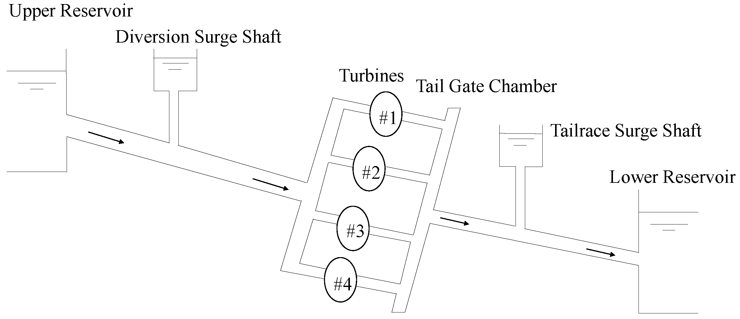
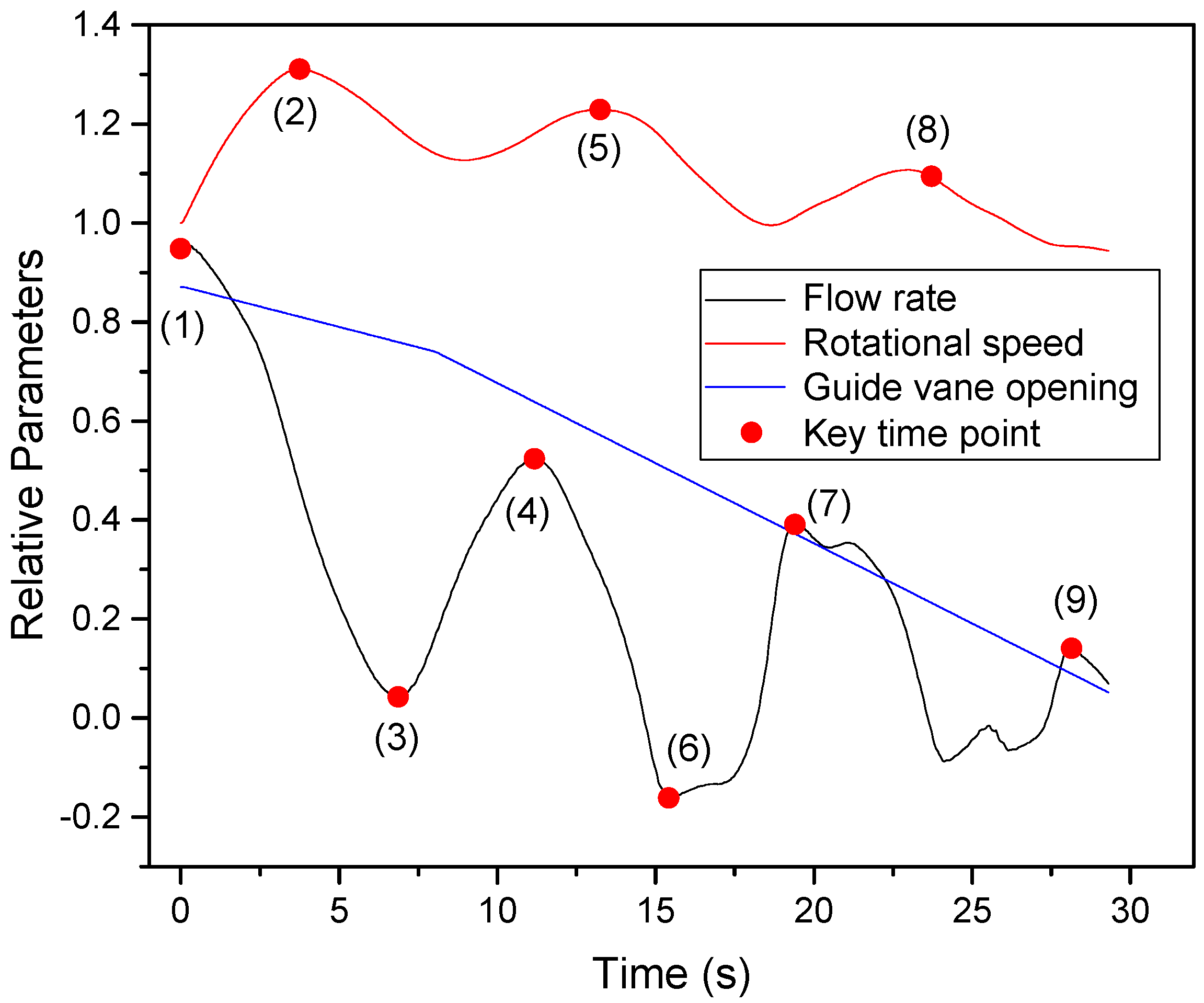
3.1. 1D Pipeline Calculation

The calculation object in this paper is a prototype pumped storage unit. The model of 1D pipeline calculation is shown in Figure 1, including upper and lower reservoir, diversion surge shaft and tailrace surge shaft, turbines and tail gate chamber. The basic parameters of the unit are shown in

Table 1. Parameters of the unit.

Parameter	Unit	Value
Unit capacity	MW	300
Rated speed $N_r$	rpm	500
Number of stay vanes		20
Number of guide vanes		20
Number of runner blades		7

. The scope of 1D calculation includes the upstream reservoir to the downstream reservoir and the scope of 3D CFD calculation is the turbine part of the system, including flow domains of the spiral case, stay vane, guide vane, runner, draft tube, upper and lower labyrinth seals and balance tubes. The further FEM calculation includes the head cover, stay ring and bottom ring of the unit.

The relative flow rate, relative rotational speed and relative opening curves with time are obtained by 1D calculation as shown in Figure 2 (drawn by the Origin software). Since flow rate and rotational speed are the main factors that affect the intense changes in the flow field and pressure characteristics during load rejection [5,6], the representative extreme value points in the curves of flow rate and rotational speed are selected as key time points for 3D flow field simulations and the study [10] has adopted a similar method to perform the flow field simulation.

The pressures at the spiral case inlet and the draft tube outlet calculated by 1D simulation are shown in Figure 3. The pressure values at different moments are set as the inlet and outlet boundary conditions for the 3D flow calculation.

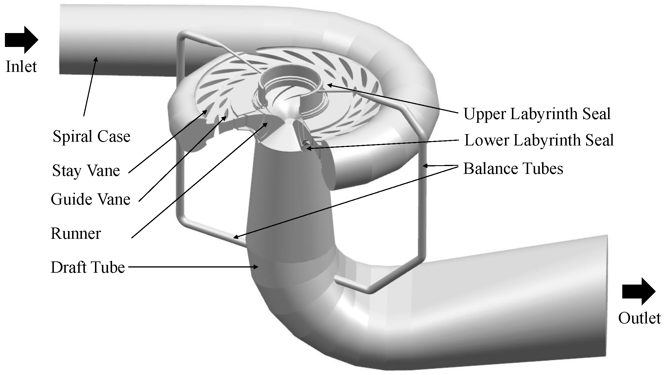
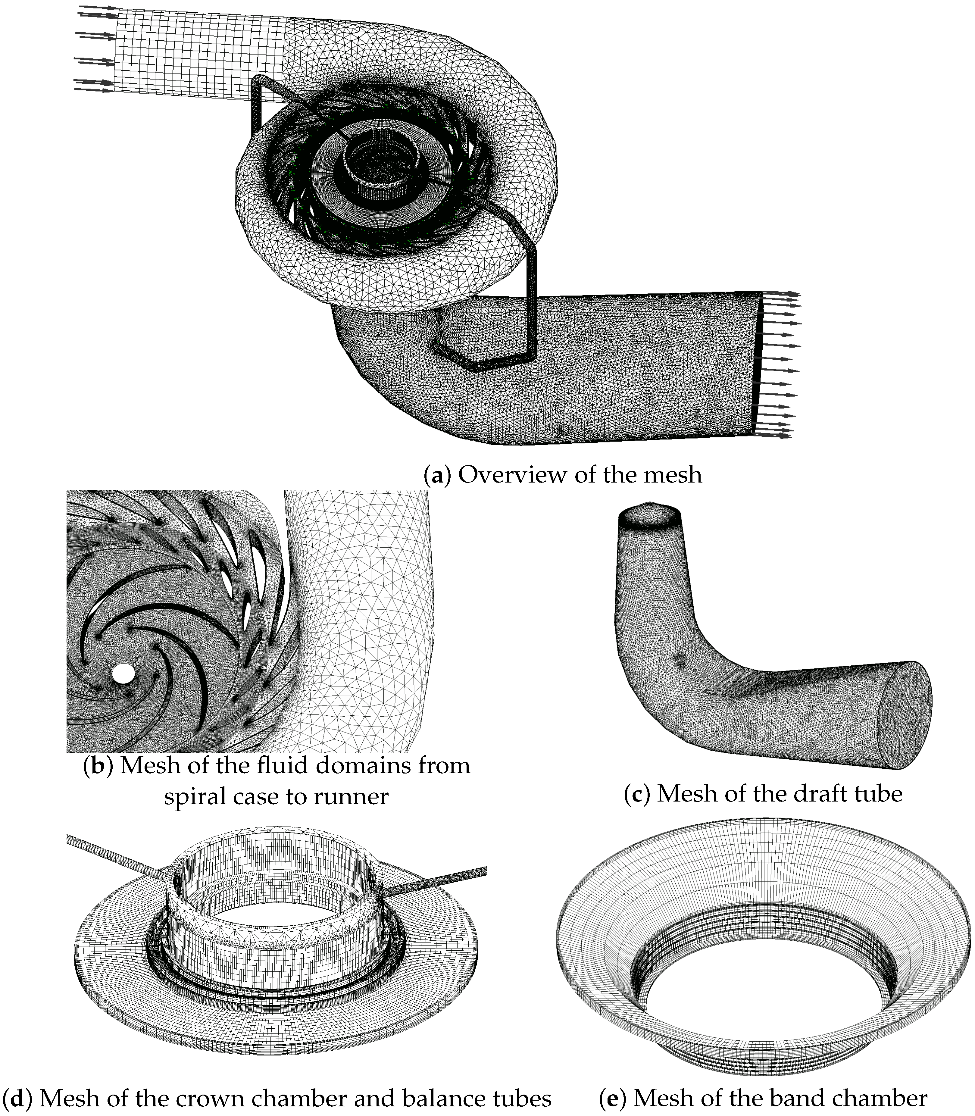
3.2. 3D Flow Calculation Model

The 3D model of the PT unit is shown in Figure 4, including spiral case, stay vane, guide vane, runner, draft tube, upper and lower labyrinth seals and balance tubes. The size of labyrinth seal clearance is only 1.5 mm, which has a significant impact on the flow of the unit; therefore, the upper and lower clearances are considered in the model of the fluid domain.

The details of the section from the unit spiral case to the draft tube are shown in Figure 5. Pressure monitoring points (C1, C2, V1, V2, B1, B2) are set at the upper and lower labyrinth seals and the vaneless area.

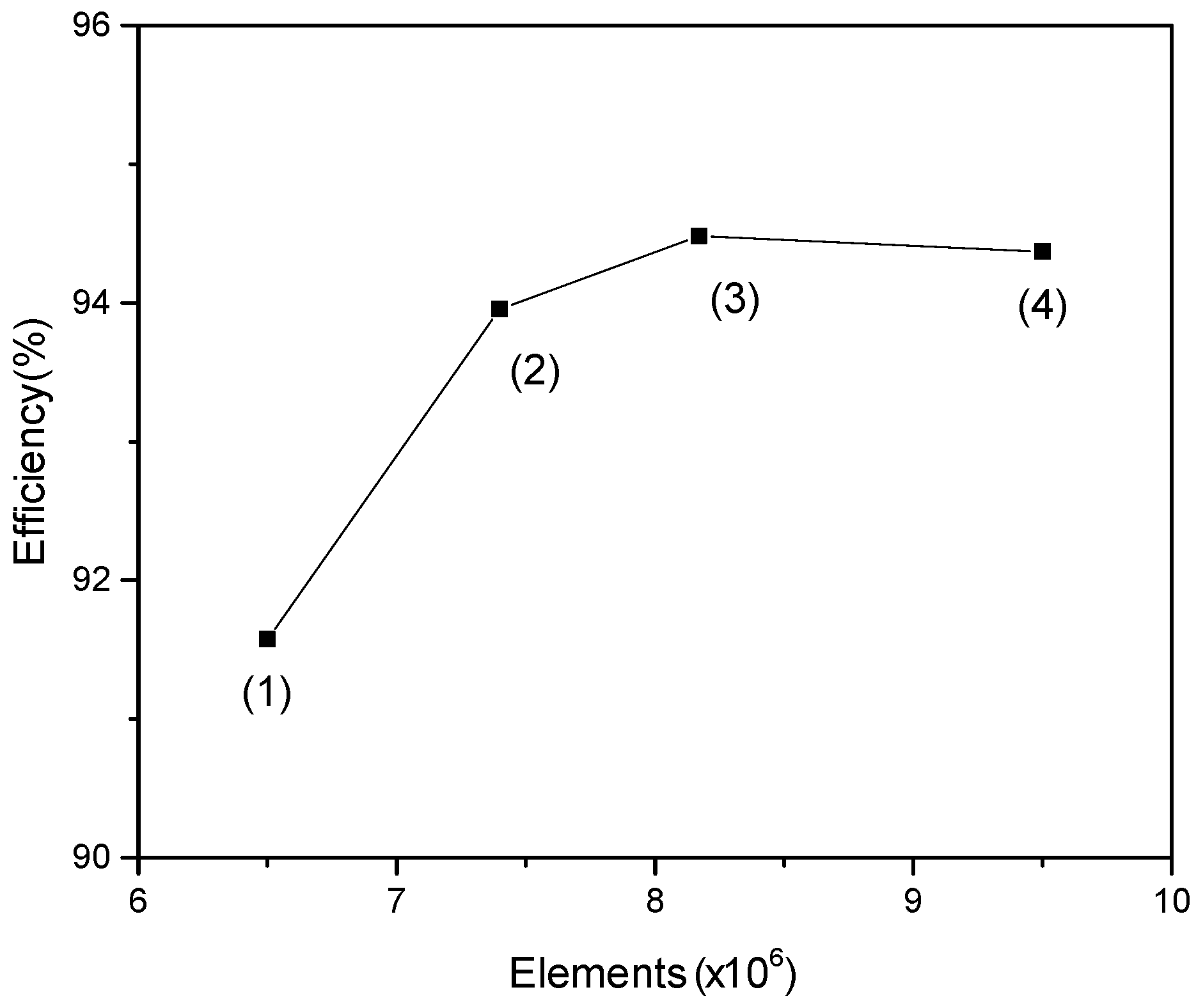
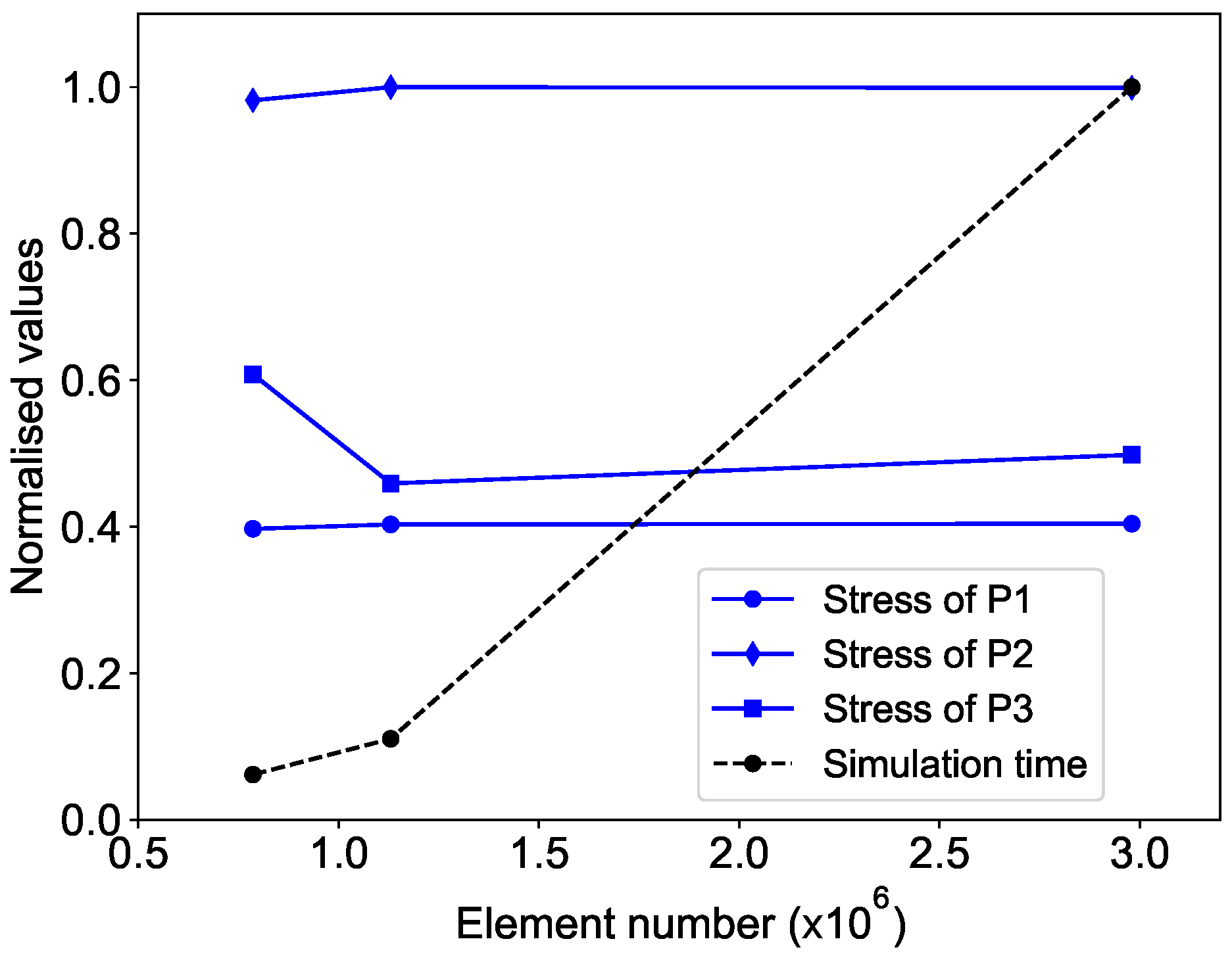
3.3. Mesh Independence Analysis of the 3D Flow Calculation

ANSYS CFX was used to carry out the 3D CFD analysis. The analysis type was set to stable and the discrete format and the solver were set to high resolution. The runner domain was set to rotate at an angular velocity of 500 rpm. The wall condition was set as non-slip wall. The interfaces between guide vanes and runner, runner and draft tube were set to Frozen Rotor and the others are set to General Connection. The turbulence model was set to shear stress transport, the turbulence model was set to shear stress transfer and the turbulence mathematical accuracy was set to first order with a convergence residual of ${10}^{-5}$.

The mesh quality is very important for 3D turbulence calculation. In this paper, the tetrahedron–hexahedron hybrid mesh was used to discrete the fluid domain. In ANSYS Workbench, an automatic mesh generating method according to different guide vane openings was set up to ensure the uniformity of mesh size of guide vane under a given opening. The fluid domain mesh of the PT unit is shown in Figure 6.

In this paper, four sets of meshes with different element sizes were created to calculate the steady-state of full-load condition (point (1) in Figure 3). The mesh independence analysis was carried out by comparing the calculated efficiencies with different set of meshes (Figure 7). The final adopted mesh (3) of the PT unit for load rejection calculation is shown in

Table 2. Element number of flow domains.

Flow Domain	Elements ($\times {10}^6$)
Spiral case & Stay vane	3.26
Guide Vane	0.27
Runner	3.63
Draft tube	0.60
Labyrinth seal & Balance tubes	0.40
Total	8.16

.

3.4. Results and Discussion of the 3D Flow Calculation

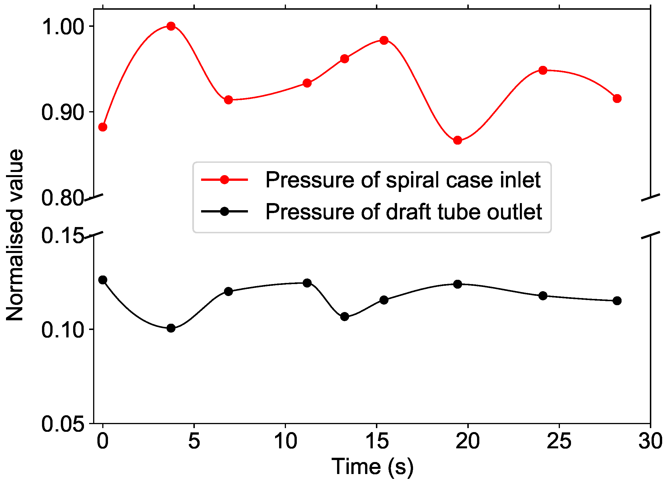
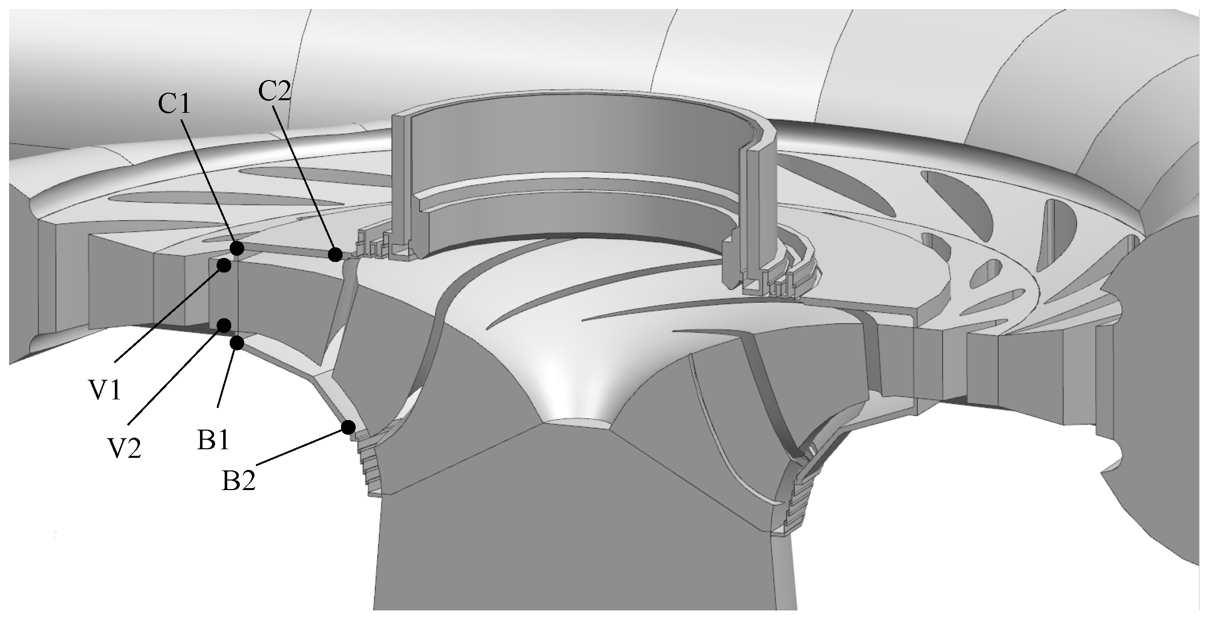
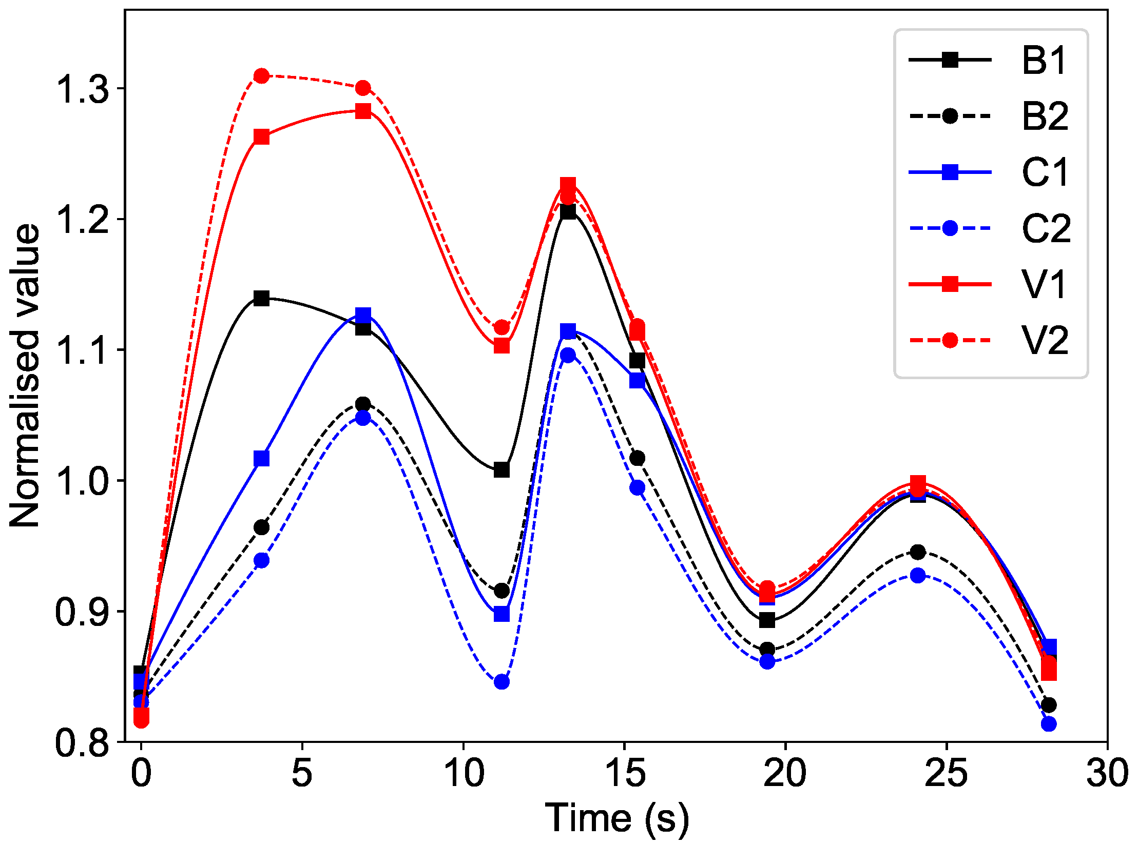
3.4.1. Pressure Change at the Monitoring Points

Figure 8 shows the pressure change of the monitoring points in the calculation. The pressures at various monitoring points fluctuate violently during load rejection, which is closely related to the flow rate and rotational speed of the unit. High rotational speed enhances the shear effect of the runner on the non-rotating flow region and increases the water flow velocities at the runner inlet and the upstream, resulting in more wake cutting on the guide vane flow domain. It also intensifies rotor–stator interaction phenomena and increases pressure pulsation in the vaneless area (t = 3.74 s, t = 13.24 s and t = 24.10 s). In addition, at the moment t = 6.88 s, the opening of the guide vane is large, the rotational speed is high and the flow rate is low, the flow separation and vortices of the incoming flow from the guide vane increase and a large number of blade passage vortices appear in the runner, which are extremely unstable. The irregular flow leads to increased energy dissipation and increased pressure near the vaneless area. In the case of a high flow rate and low rotational speed (t = 11.19 s and t = 19.43 s), the direction of the outflow velocity of the guide vane deviates less from the design operating condition, so the flow inside the unit is more adequate and uniform and the pressure shows a lower level.

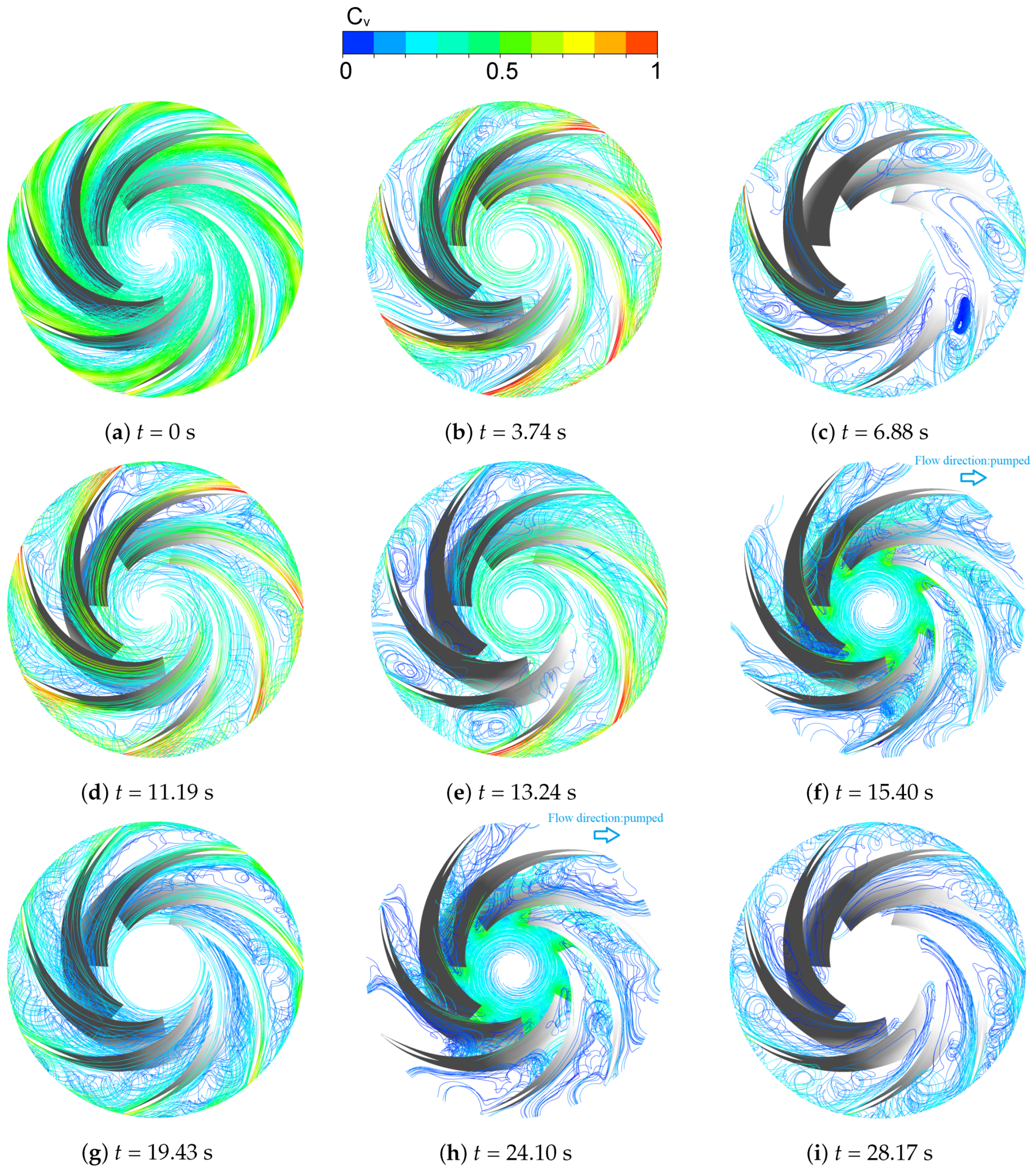
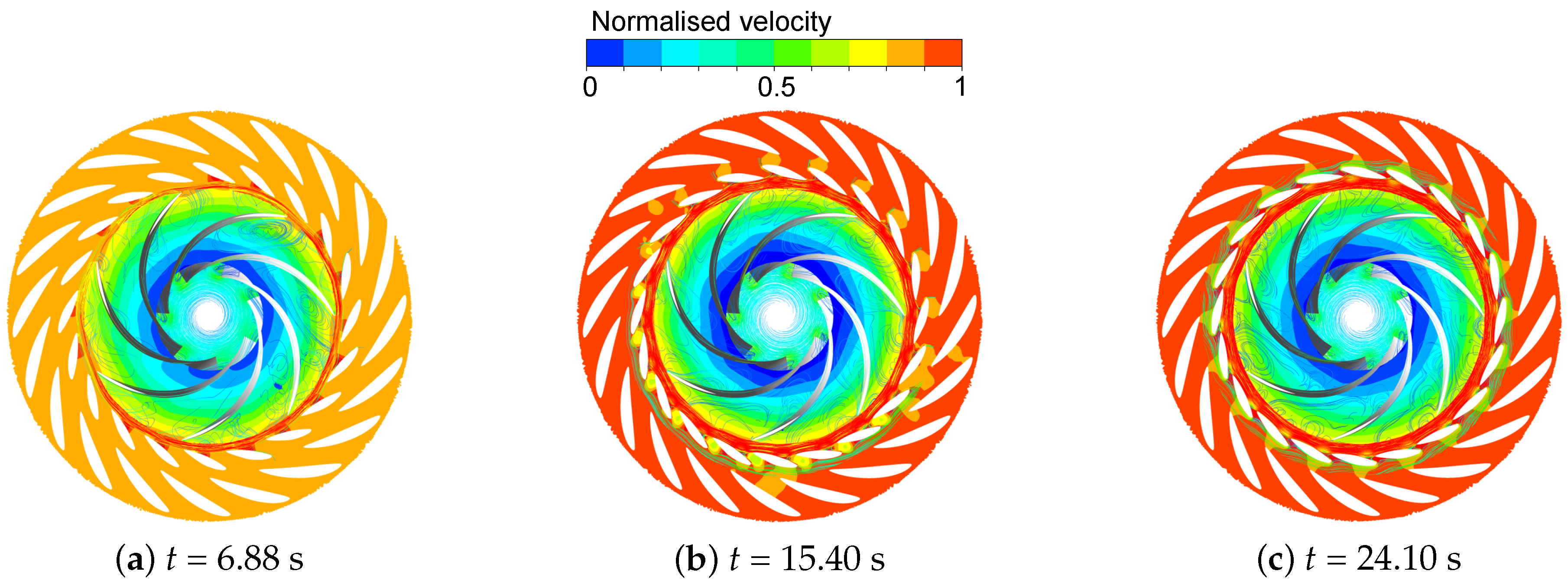
3.4.2. Flow Pattern Change in the Runner Passage

In the process of load rejection, the flow from the guide vane to the runner outlet shows extremely unstable turbulent characteristics. Figure 9 shows the streamline distribution in the runner in the whole load rejection process. When the load rejection does not begin (t = 0 s), the flow in the runner is uniform. Afterward, the flow is greatly affected by the changes in flow rate, head and speed.

At the moments when the flow rate is high (t = 3.74 s, 11.19 s, 13.24 s, 19.43 s), largescale blade duct vortices appear on the suction surface of the blade due to the peak or high rotational speed. The size of the blade passage vortices corresponds to the size of the flow duct, which disturbs the flow of the whole unit and makes the hydraulic torque of the runner fluctuate violently with the pressure of the unit.

At the moments with negative flow (t = 15.40 s and 24.10 s), the unit enters the reverse pump operating condition. Due to the imbalance of speed and flow, the flow between blade passages rotates abnormally and separated flow occurs on the pressure surface of the runner. Both factors cause the wake falling off upstream of the runner blades and a large number of swirl eddies appear in the vaneless area. At the same time, wake falling off also occurs at the leading edge of the guide vanes and stay vanes. The unstable flow of the unit extends to the spiral case area. It is shown in research [15] that the vortex core in the vaneless area is impacted instantaneously by a large number of reverse refluxes into the guide vane area and the stay vane area when the unit experiences the reverse pump operating condition, which is also in accordance with the calculation results in this paper.

3.4.3. Pressure Change in the Flow Passages

Figure 10 shows the pressure change of head cover during load rejection. At the starting moment (t = 0 s) and the moments (t = 3.73 s, 11.19 s, 13.24 s, 19.43 s) when the hydraulic moment is positive or equal to zero, the pressure distribution of the unit is relatively uniform. The pressure difference between the pressure surface of the runner and the suction surface is obvious without pressure concentration.

At the time (t = 6.88 s, 15.40 s, 24.10 s) when the hydraulic torque is negative, the pressure difference between the pressure surface and suction surface disappears and obvious pressure concentration points appear at guide vanes near the flow clearances.

Figure 11 shows the streamline distribution from the runner to the guide vane, with obvious flow separation at the pressure concentration point and strong circulation behind the guide vane. Pressure concentration is caused by the separation of high-speed annular flow through a small flow gap, resulting in a sudden drop in velocity and local pressure rise as the flow energy is converted into impact on the edge of the vanes.

4. Fluid–Structure Coupling Analysis of the Stationary Structures

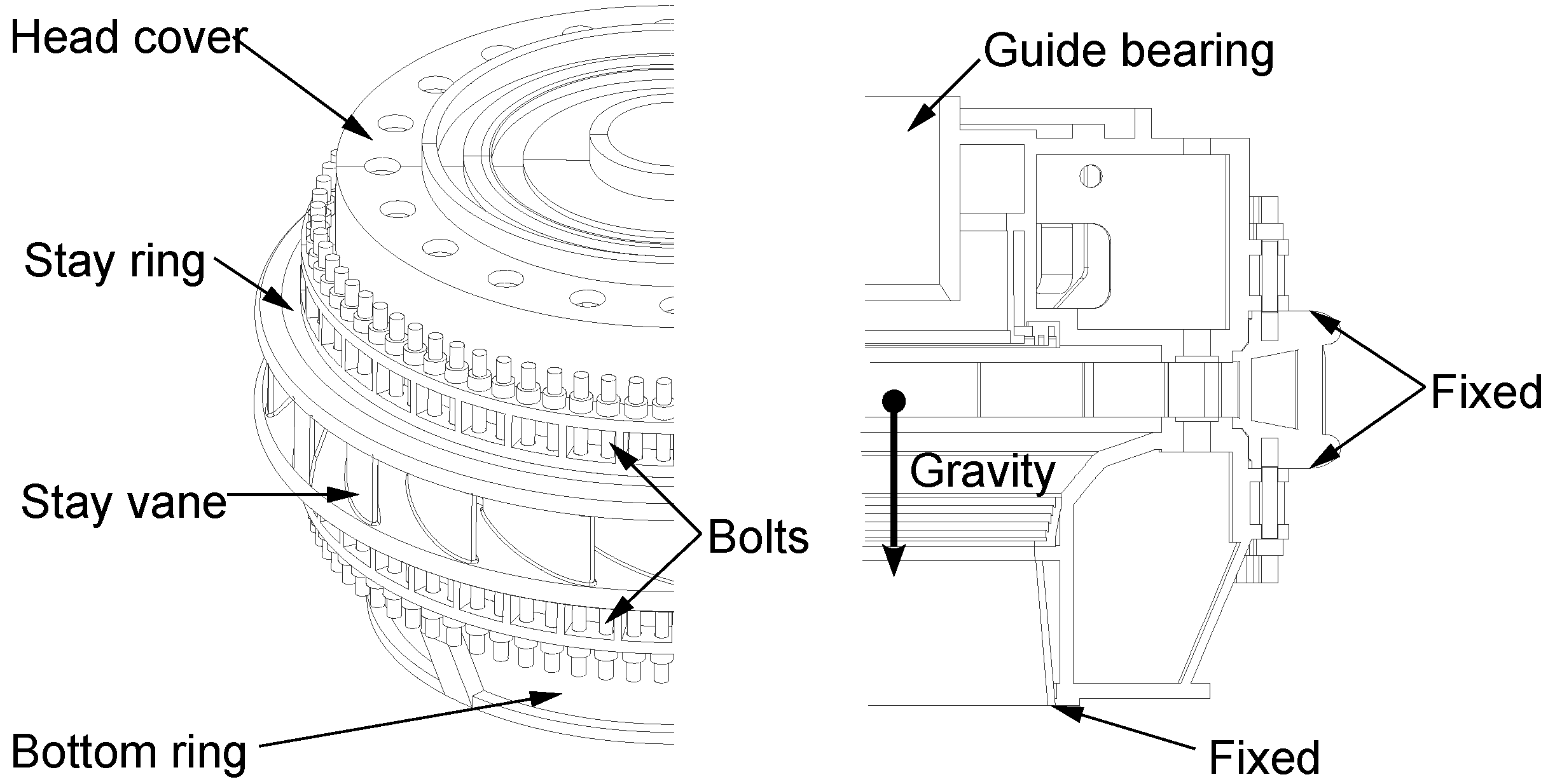
4.1. Simulation Model and Boundary Conditions

Figure 12 demonstrates the CAD model and boundary conditions of the stationary structure of the PT unit. The head cover, the stay ring and the bottom ring were bolted together as a single structure. The equivalent stiffness coefficient of the turbine guide bearing was set as 1 × ${10}^9$ N·m${}^{-1}$ and the standard gravity was taken into consideration. Since the thrust bearing structure supporting the entire rotating system was directly placed on the head cover, the equivalent mass of them was applied to the head cover. The upper and lower surfaces of the stay ring were fixed in concrete and the bottom surface of the bottom ring was welded to the draft tube cone. ANSYS Mechanical was used to carry out the fluid–structure coupling analysis.

The material and mechanical properties of the research object were configured according to

Table 3. Material properties of the structures.

	Structures
Density [kg·m${}^{-3}$]	7850
Elastic modulus [MPa]	2.1 × ${10}^5$
Poisson’s ratio [-]	0.3

.

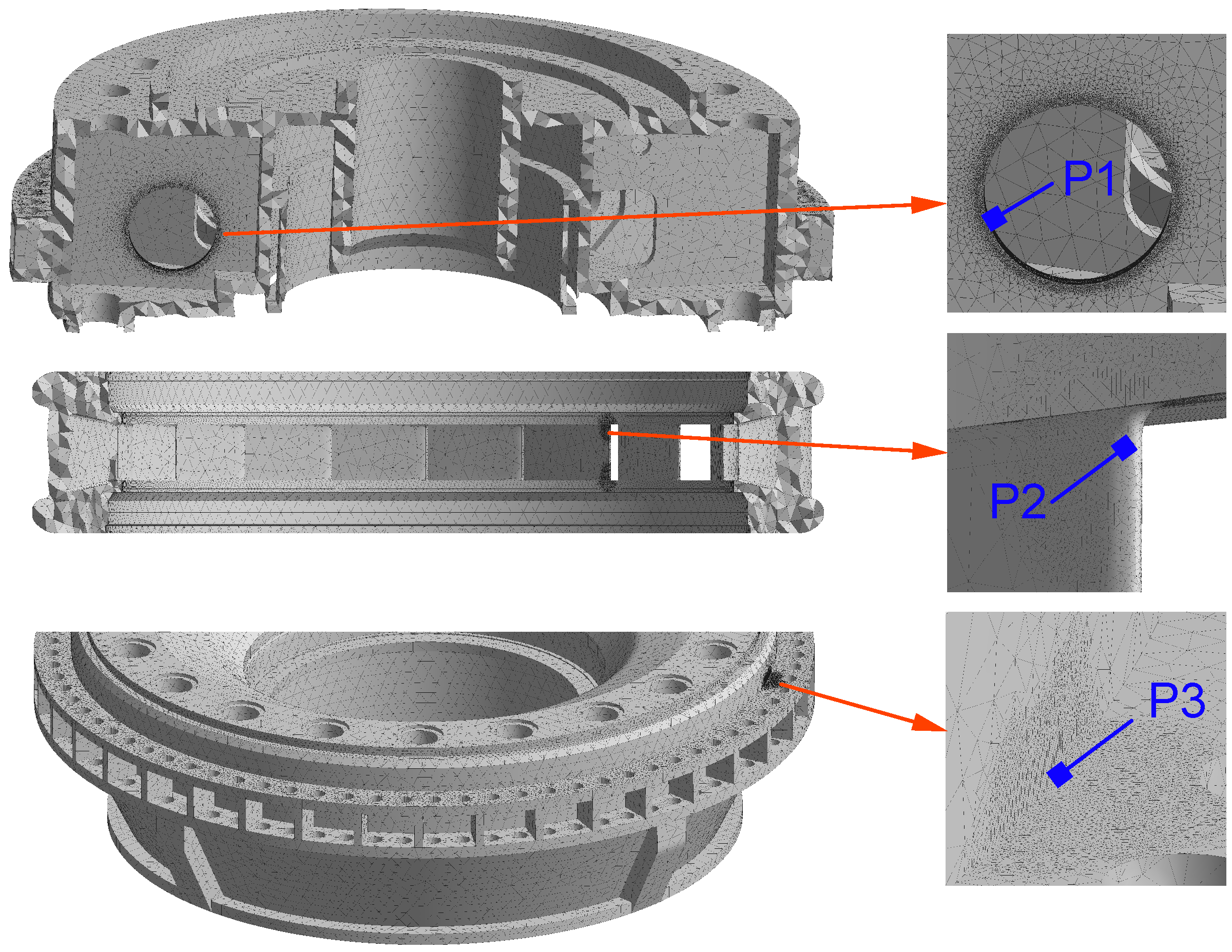
4.2. Mesh Sensitivity Study

As shown in Figure 13, the structural models were meshed using high-quality tetrahedral elements, better suited for complex geometries. The meshes were refined for the typical stress concentration areas of the head cover, stay ring and bottom ring (P1, P2 and P3).

The element size has a significant effect on the FEA results, so it is reasonable to conduct a mesh sensitivity study to obtain a set of mesh that provides a good balance between computational time and the accuracy of the results. Figure 14 presents the simulation duration and convergence of the simulation results for three sets of meshes with different sizes of elements. The element numbers of three sets of meshes are 7.86 × ${10}^5$, 1.13 × ${10}^6$ and 2.97 × ${10}^6$, respectively. Compared to the third set mesh where the element size was significantly reduced, the simulation results of the second set mesh show negligible changes, but the computational time was only 1/9 of the third one; therefore, we conclude that the second set mesh has converged and can be used for further analysis to save calculation time.

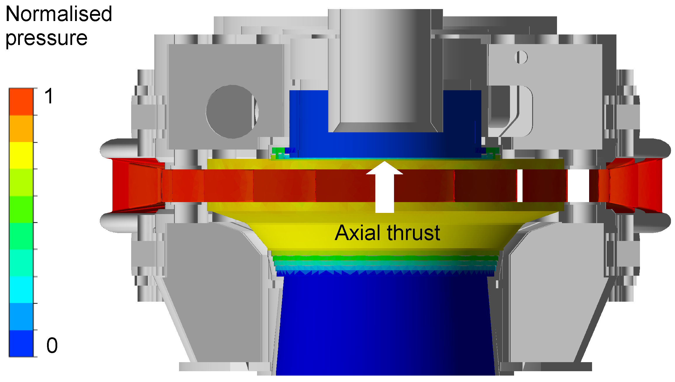
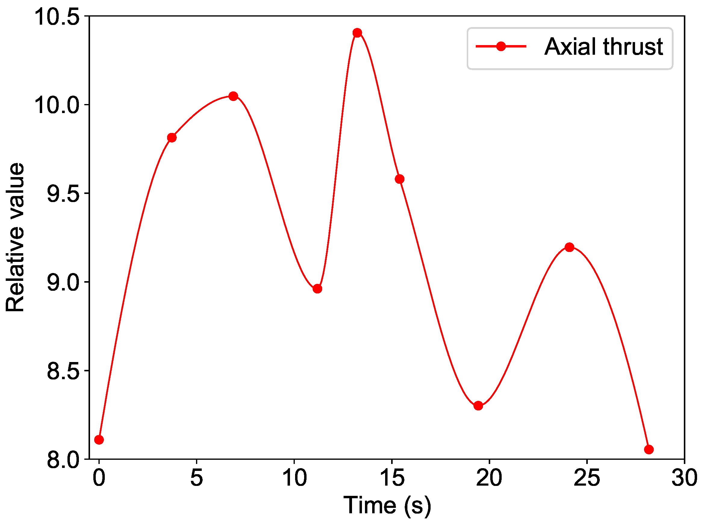
4.3. Fluid Pressure Mapping and Axial Thrust Analysis

To perform the fluid–structure coupling analysis, the pressure distributions acting on the stationary structures at different time points during load rejection were exported from the 3D CFD analysis described earlier. Each pressure file includes the 3D coordinates and the pressure values of the nodes on the fluid–structure coupling interface in the form of (x, y, z, Pressure). Since the structural mesh is different from the fluid mesh on the fluid–structure coupling interface, the fluid nodal pressure values need to be interpolated and mapped onto the nearest nodes of the structures according to the distance between the fluid and structure nodes. The ANSYS built-in tool can complete this task precisely and flawlessly.

Figure 15 shows the mapped pressure distribution on the stationary structures of the PT unit at a given moment in time. By applying the pressure files sequentially to the structural model during load rejection, the flow-induced deformation and stress of the stationary components including the head cover, stay ring and bottom ring can be calculated.

The huge hydraulic pressures acting on the stationary structures of the PT unit lifted the head cover and the upper part of the stay ring and pressed down the bottom ring and the lower part of the stay ring. In addition, rapidly changing pressure loads during load rejection generated large stresses on the head cover, stay vanes and bottom ring.

The axial thrust on the head cover during load rejection needs to be carefully investigated as it causes axial vibration of the head cover, the thrust bearing structure and the entire rotating system. Figure 16 illustrates the relative axial thrust of the head cover during load rejection, which was calculated by dividing the head cover axial thrust by the total mass of the head cover, the thrust bearing structure and the rotating system. The positive direction of the head cover axial thrust is axially upward and the value of the axial thrust varies greatly with time during load rejection, reaching a maximum value at t = 13.24 s, which is more than 10 times the total gravity of the head cover, the thrust bearing structure and the rotating system.

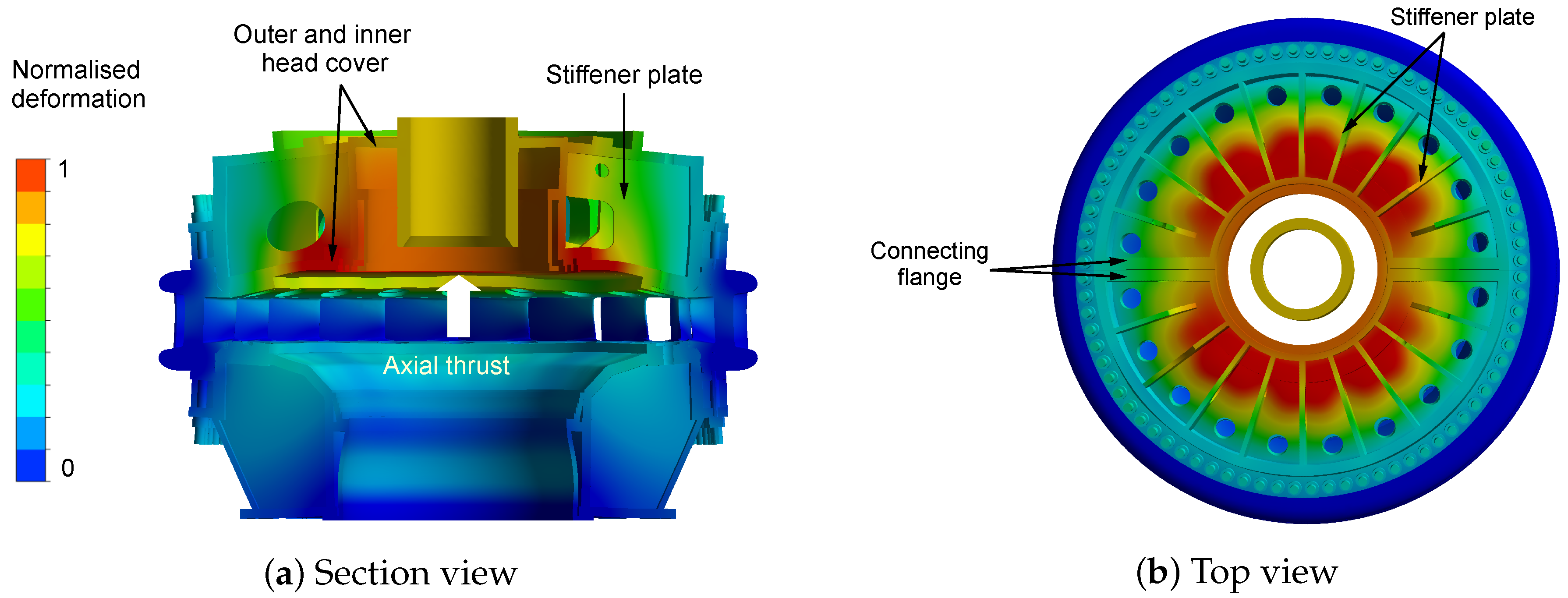
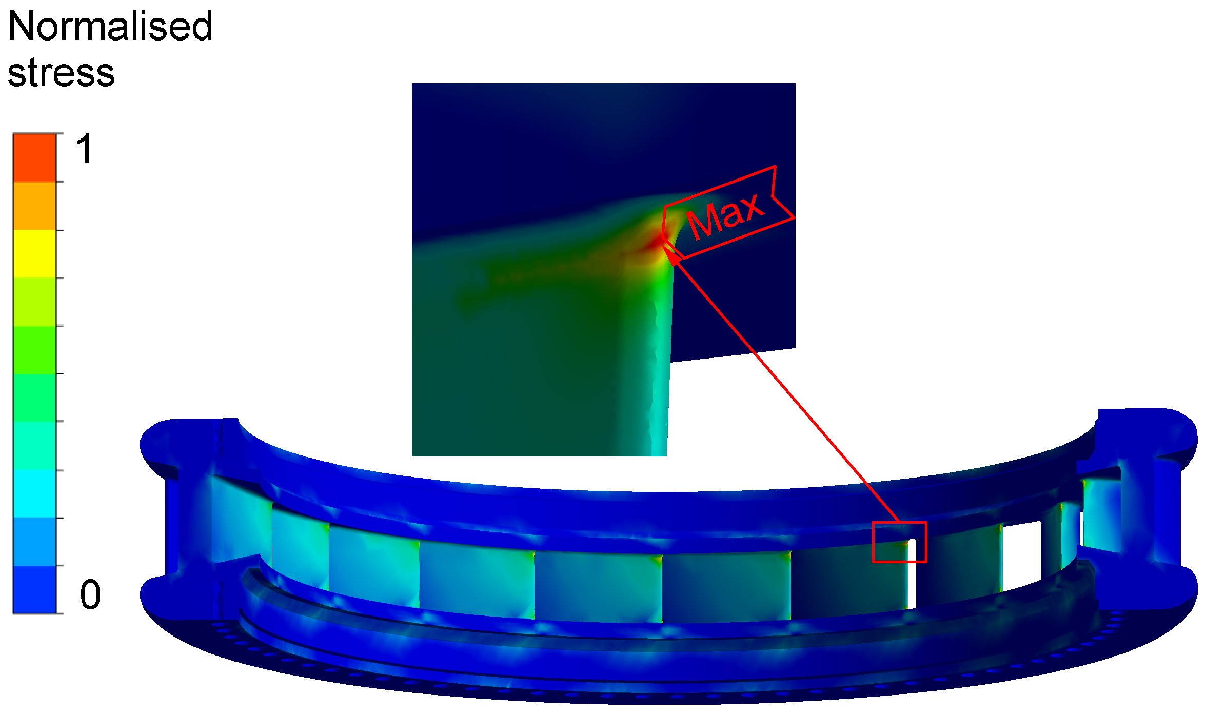
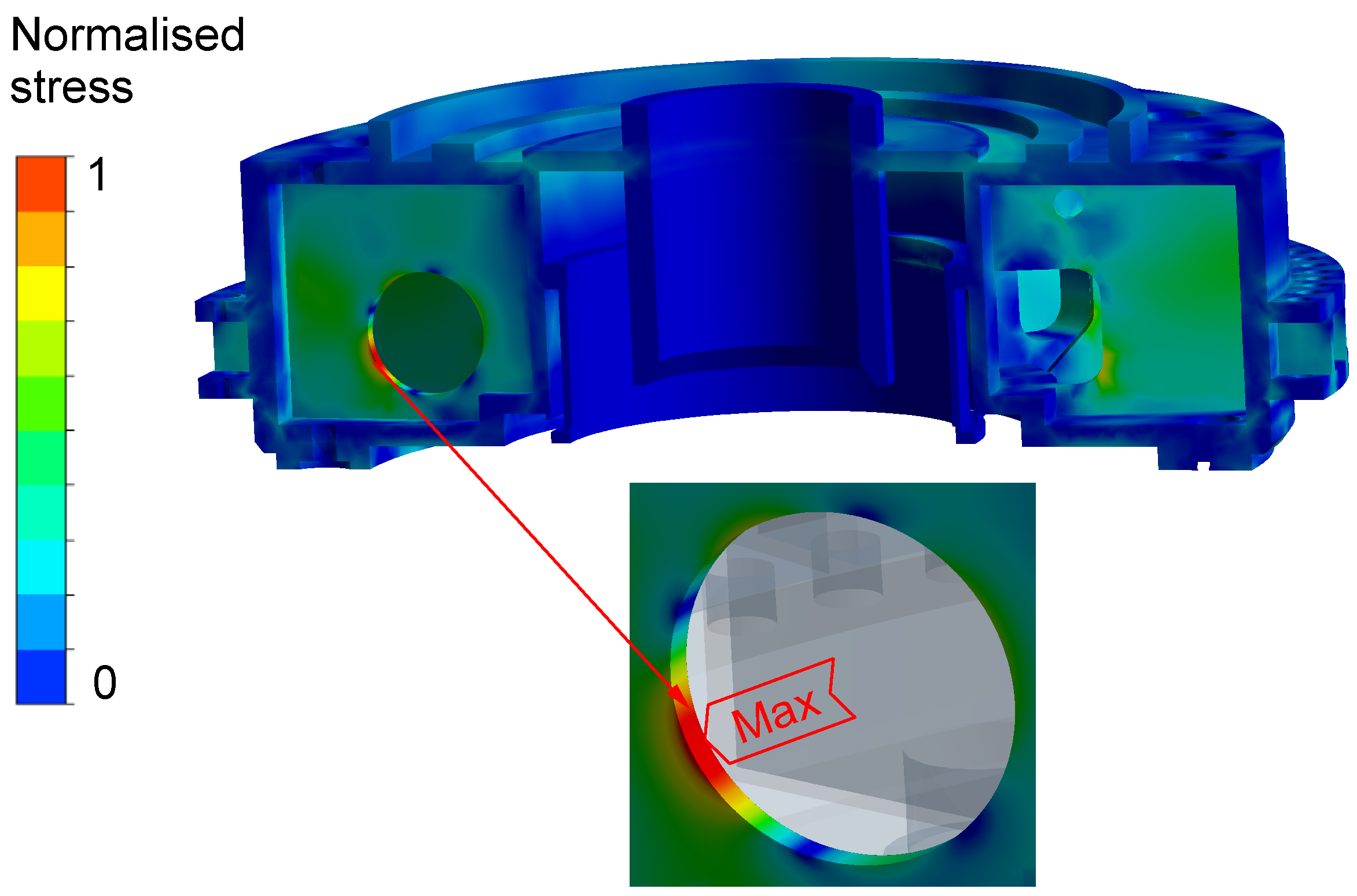
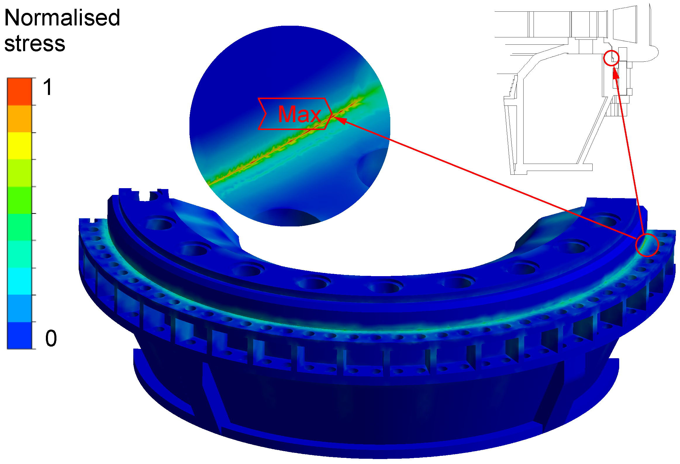
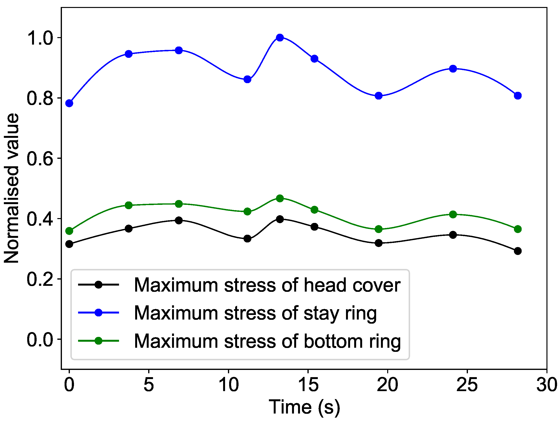
4.4. Results and Discussion

Figure 17 shows the total deformation distribution of the stationary structures caused by the fluid flow in the PT unit during load rejection. The head cover consists of an outer and an inner cover, 4 connecting flanges and 18 stiffener plates with different shaped openings. The huge hydraulic pressure of the fluid acting on the inner surface of the head cover resulted in a large axial thrust, which caused relatively large deformation on the head cover and the largest deformation appeared on the inner head cover where there is no support in the axial direction. The bottom ring is reinforced by 18 stiffener plates and its axial force area is much smaller than that of the head cover, so the total deformation of the bottom ring is at a low level. The stay ring is shorter and stiffer than the head cover and the bottom ring and has a much smaller axial force area, so the flow-induced deformation of the stay ring is also small.

Figure 18 shows the flow-induced stress distribution of the stationary structures.

The fluid pressure on the inner surface of the stationary structures pushes the head cover upward and the bottom ring downward. The stay ring between the head cover and the bottom ring is stretched and the maximum stress occurs on the trailing edge fillet of a guide vane of the stay ring (Figure 19).

The head cover is only supported by the stay ring in the axial direction but has a large area facing the high pressure water. The stiffener plates are welded between the inner and outer head cover to increase the stiffness and effectively reduce the deformation of the head cover caused by the pressure; however, different shaped openings and holes are made in the stiffener plates for installing various pipes such as pressure balance pipes, cooling water pipes and pressure measurement pipes. The normalized stress distribution of the head cove relative to its maximum stress value is shown in Figure 20, which shows that the hot spots of head cover during load rejection appear on the different shaped openings of the stiffener plates and the maximum stress occurs on the bottom-right side of the circular opening.

Figure 21 illustrates the stress distribution of the bottom ring during load rejection. The stresses are normalized with reference to the maximum stress value of the bottom ring and the maximum stress of the bottom ring occurs on the corner of the bottom ring flange.

The von Mises stress distributions of the stationary structures at different time points during load rejection are similar and the hot spots of the stationary structures appear in the same locations of the head cover, stay ring and bottom ring, but the maximum stress value change with time. Figure 22 shows the stress comparison of the normalized stresses of the stationary structures during load rejection. All stresses are normalized with reference to the maximum stress of the stay ring, which is larger than the maximum stresses of the head cover and the bottom ring.

The stresses are normalized with reference to the maximum stress value of the bottom ring.

The comparison of the axial thrust force on the head cover and the normalized maximum stresses of the stationary structures during load rejection is demonstrated in Figure 23. The tendency of these there parameters follows the same pattern. The maximum stress values of the head cover, stay ring and bottom ring change with the axial thrust force on the head cover and reached the respective maximum value at t = 13.24 s.

5. Conclusions

This study has carried out the fluid dynamic analysis and the flow-induced structural behaviour analysis of a prototype reversible pump turbine unit during the load rejection based on the measured data.

During the load rejection, the internal flow of the unit changes drastically and the impact of the runner on the upstream is intensified due to the rapid increase in the rotational speed and the flow variation from the design condition leads to more flow separation and energy dissipation at the guide vane outlet. The high rotational speed and the sudden change of flow rate are the main reasons for the unstable flow and pressure characteristics during the load rejection process and the pressure reaches local peaks at t = 3.74 s, 6.88 s, 13.24 s and 24.10 s.

When the unit enters the reverse pump working condition ( t = 15.40 s and 24.10 s), the drastic changes in flow rate, speed and guide vane opening lead to a strong circulation in front of the guide vanes. The water flow through the guide vanes is separated from the circulating flow, resulting in strong local pressures at the backside of the guide vanes.

The pressure change in the flow domains of the spiral case and guide vane during load rejection has the same trend as the pressure at the spiral case outlet. The pressure acting on head cover changed largely during load rejection and reached the maximum value at t = 13.24 s.

The huge hydraulic forces of the pump turbine unit during load rejection cause large time-varying stresses on the stationary structures of the pump turbine unit. The maximum stress of the stationary structures including the head cover, stay ring and bottom ring at different time points during load rejection are strongly correlated with that of axial thrust force on the head cover and reached the maximum values at t = 13.24 s.

The maximum deformation of the stationary structures during the load rejection occurs on the inner edge of the head cover closed to the main shaft and the maximum equivalent stress is located at the fillet of the stay vane trailing edge.

These findings contribute to an improved physical understanding of the flow characteristics and structural behaviour of the stationary structures of similar pump turbines, Francis turbines and centrifugal pumps and help engineers to better design the turbine units that can operate safely and stably.

References

1. Liu, X.; Luo, Y.; Wang, Z. A review on fatigue damage mechanism in hydro turbines. Renew. Sustain. Energy Rev. 2016, 54, 1–14. [Google Scholar] [CrossRef]
2. Casanova, F.; Mantilla, C. Fatigue failure of the bolts connecting a Francis turbine with the shaft. Eng. Fail. Anal. 2018, 90, 1–13. [Google Scholar] [CrossRef]
3. Peltier, R.; Boyko, A.; Popov, S.; Krajisnik, N. Investigating the Sayano-Shushenskaya Hydro Power Plant Disaster. Power 2010, 154, 48. [Google Scholar]
4. Egusquiza, E.; Valero, C.; Huang, X.; Jou, E.; Guardo, A.; Rodriguez, C. Failure investigation of a large pump-turbine runner. Eng. Fail. Anal. 2012, 23, 27–34. [Google Scholar] [CrossRef] [Green Version]
5. Mandair, S.; Morissette, J.F.; Magnan, R.; Karney, B. MOC-CFD coupled model of load rejection in hydropower station. IOP Conf. Ser. Earth Environ. Sci. 2021, 774, 012021. [Google Scholar] [CrossRef]
6. Zhou, D.; Chen, H.; Kan, K.; Yu, A.; Binama, M.; Chen, Y. Experimental study on load rejection process of a model tubular turbine. IOP Conf. Ser. Earth Environ. Sci. 2021, 774, 012036. [Google Scholar] [CrossRef]
7. Bi, H.; Chen, F.; Wang, C.; Wang, Z.; Fan, H.; Luo, Y. Analysis of dynamic performance in a pump-turbine during the successive load rejection. IOP Conf. Ser. Earth Environ. Sci. 2021, 774, 012152. [Google Scholar] [CrossRef]
8. Zhang, H.; Su, D.; Guo, P.; Zhang, B.; Mao, Z. Stochastic dynamic modeling and simulation of a pump-turbine in load-rejection process. J. Energy Storage 2021, 35, 102196. [Google Scholar] [CrossRef]
9. He, L.Y.; Wang, Z.W.; Kurosawa, S.; Nakahara, Y. Resonance investigation of pump-turbine during startup process. IOP Conf. Ser. Earth Environ. Sci. 2014, 22, 32024. [Google Scholar] [CrossRef] [Green Version]
10. Kolšek, T.; Duhovnik, J.; Bergant, A. Simulation of unsteady flow and runner rotation during shut-down of an axial water turbine. J. Hydraul. Res. 2006, 44, 129–137. [Google Scholar] [CrossRef]
11. Ciocan, G.D.; Iliescu, M.S.; Vu, T.C.; Nennemann, B.; Avellan, F. Experimental Study and Numerical Simulation of the FLINDT Draft Tube Rotating Vortex. J. Fluids Eng. 2006, 129, 146–158. [Google Scholar] [CrossRef]
12. Huang, X.; Oram, C.; Sick, M. Static and dynamic stress analyses of the prototype high head Francis runner based on site measurement. IOP Conf. Ser. Earth Environ. Sci. 2014, 22, 032052. [Google Scholar] [CrossRef] [Green Version]
13. Goyal, R.; Cervantes, M.J.; Gandhi, B.K. Characteristics of Synchronous and Asynchronous modes of fluctuations in Francis turbine draft tube during load variation. Int. J. Fluid Mach. Syst. 2017, 10, 164–175. [Google Scholar] [CrossRef]
14. Nicolet, C.; Alligne, S.; Kawkabani, B.; Simond, J.-J.; Avellan, F. Unstable Operation of Francis Pump-Turbine at Runaway: Rigid and Elastic Water Column Oscillation Modes. Int. J. Fluid Mach. Syst. 2009, 2, 324–333. [Google Scholar] [CrossRef] [Green Version]
15. Fu, X.; Li, D.; Wang, H.; Zhang, G.; Li, Z.; Wei, X. Dynamic instability of a pump-turbine in load rejection transient process. Sci. China Technol. Sci. 2018, 61, 1765–1775. [Google Scholar] [CrossRef]
16. Mao, Z.; Tao, R.; Bi, H.; Luo, Y.; Wang, Z. Numerical study of hydraulic axial force of prototype pump-turbine pump mode’s stop with power down. IOP Conf. Ser. Earth Environ. Sci. 2021, 774, 012094. [Google Scholar] [CrossRef]
17. Li, X.; Mao, Z.; Lin, W.; Bi, H.; Tao, R.; Wang, Z. Prediction and Analysis of the Axial Force of Pump-Turbine during Load-Rejection Process. IOP Conf. Ser. Earth Environ. Sci. 2020, 440, 052081. [Google Scholar] [CrossRef] [Green Version]
18. Walseth, E.C.; Nielsen, T.K.; Svingen, B. Measuring the Dynamic Characteristics of a Low Specific Speed Pump—Turbine Model. Energies 2016, 9, 199. [Google Scholar] [CrossRef] [Green Version]
19. Avdyushenko, A.Y.; Cherny, S.G.; Chirkov, D.V.; Skorospelov, V.A.; Turuk, P.A. Numerical simulation of transient processes in hydroturbines. Thermophys. Aeromech. 2013, 20, 577–593. [Google Scholar] [CrossRef]
20. Liu, X.; Liu, C. Eigenanalysis of Oscillatory Instability of a Hydropower Plant Including Water Conduit Dynamics. IEEE Trans. Power Syst. 2007, 22, 675–681. [Google Scholar] [CrossRef]
21. Avdyushenko, A.; Chernyi, S.; Chirkov, D. Numerical algorithm for modelling three-dimensional flows of an incompressible fluid using moving grids. Comput. Technol. 2012, 17, 3–25. [Google Scholar]
22. Widmer, C.; Staubli, T.; Ledergerber, N. Unstable Characteristics and Rotating Stall in Turbine Brake Operation of Pump-Turbines. J. Fluids Eng. 2011, 133, 041101. [Google Scholar] [CrossRef]
23. Nicolle, J.; Giroux, A.M.; Morissette, J.F. CFD configurations for hydraulic turbine startup. IOP Conf. Ser. Earth Environ. Sci. 2014, 22, 032021. [Google Scholar] [CrossRef]
24. Mao, Z.; Tao, R.; Chen, F.; Bi, H.; Cao, J.; Luo, Y.; Fan, H.; Wang, Z. Investigation of the Starting-Up Axial Hydraulic Force and Structure Characteristics of Pump Turbine in Pump Mode. J. Mar. Sci. Eng. 2021, 9, 158. [Google Scholar] [CrossRef]
25. Münch, C.; Ausoni, P.; Braun, O.; Farhat, M.; Avellan, F. Fluid–structure coupling for an oscillating hydrofoil. J. Fluids Struct. 2010, 26, 1018–1033. [Google Scholar] [CrossRef]
26. Benra, F.-K.; Dohmen, H.J. Comparison of Pump Impeller Orbit Curves Obtained by Measurement and FSI Simulation. In Proceedings of the ASME Pressure Vessels and Piping Conference, San Antonio, TX, USA, 22–26 July 2007; pp. 41–48. [Google Scholar] [CrossRef]
27. Kato, C.; Yoshimura, S.; Yamade, Y.; Jiang, Y.Y.; Wang, H.; Imai, R.; Katsura, H.; Yoshida, T.; Takano, Y. Prediction of the Noise From a Multi-Stage Centrifugal Pump. In Proceedings of the Fluids Engineering Division Summer Meeting, Houston, TX, USA, 19–23 June 2005; pp. 1273–1280. [Google Scholar] [CrossRef]
28. Jiang, Y.; Yoshimura, S.; Imai, R.; Katsura, H.; Yoshida, T.; Kato, C. Quantitative evaluation of flow-induced structural vibration and noise in turbomachinery by full-scale weakly coupled simulation. J. Fluids Struct. 2007, 23, 531–544. [Google Scholar] [CrossRef]
29. Abdelsalam, S.I.; Zaher, A.Z. Leveraging Elasticity to Uncover the Role of Rabinowitsch Suspension through a Wavelike Conduit: Consolidated Blood Suspension Application. Mathematics 2021, 9, 2008. [Google Scholar] [CrossRef]
Figure 1. The 1D pipeline calculation model with 4 PT units (#1 to #4).
Energies 15 03764 g001
Figure 2. The operating parameters and 9 key time points of the PT unit during load rejection.
Energies 15 03764 g002
Figure 3. Normalized pressure at the spiral case inlet and draft tube outlet.
Energies 15 03764 g003
Figure 4. The 3D modeling of flow passage of the unit.
Energies 15 03764 g004
Figure 5. Setup of the monitoring points.
Energies 15 03764 g005
Figure 6. Mesh of the fluid domains.
Energies 15 03764 g006
Figure 7. Mesh independence analysis using four sets of meshes with different element sizes.
Energies 15 03764 g007
Figure 8. Pressure change at the monitoring points.
Energies 15 03764 g008
Figure 9. Flow pattern in the runner passage.
Energies 15 03764 g009
Figure 10. Pressure distribution in the flow passages at different key time moments.
Energies 15 03764 g010
Figure 11. The streamline distribution of the unit at three key time moments.
Energies 15 03764 g011
Figure 12. CAD model and boundary conditions of the stationary structures of the PT unit.
Energies 15 03764 g012
Figure 13. Structural mesh of the stationary structure of the PT unit.
Energies 15 03764 g013
Figure 14. Mesh sensitivity study.
Energies 15 03764 g014
Figure 15. Fluid pressure mapping on the structural structures.
Energies 15 03764 g015
Figure 16. Axial thrust of the head cover during load rejection.
Energies 15 03764 g016
Figure 17. Total deformation distribution of the stationary structures.
Energies 15 03764 g017
Figure 18. The stress distribution of the stationary structures.
Energies 15 03764 g018
Figure 19. The maximum stress of the stay ring.
Energies 15 03764 g019
Figure 20. The stress distribution of the head cover.
Energies 15 03764 g020
Figure 21. The stress distribution of the bottom ring.
Energies 15 03764 g021
Figure 22. Comparison of the maximum stresses of the stationary structures during load rejection.
Energies 15 03764 g022
Figure 23. Results comparison of the PT unit during load rejection.
Energies 15 03764 g023