A Robust Kalman Filter-Based Approach for SoC Estimation of Lithium-Ion Batteries in Smart Homes

Abstract

Battery energy systems are playing significant roles in smart homes, e.g., absorbing the uncertainty of solar energy from root-top photovoltaic, supplying energy during a power outage, and responding to dynamic electricity prices. For the safe and economic operation of batteries, an optimal battery-management system (BMS) is required. One of the most important features of a BMS is state-of-charge (SoC) estimation. This article presents a robust central-difference Kalman filter (CDKF) method for the SoC estimation of on-site lithium-ion batteries in smart homes. The state-space equations of the battery are derived based on the equivalent circuit model. The battery model includes two RC subnetworks to represent the fast and slow transient responses of the terminal voltage. Moreover, the model includes the nonlinear relationship between the open-circuit voltage (OCV) and SoC. The proposed robust CDKF method can accurately estimate the SoC in the presence of the time-varying model uncertainties and measurement noises. Being able to cope with model uncertainties and measurement noises is essential, since they can lead to inaccurate SoC estimations. An experiment test bench is developed, and various experiments are conducted to extract the battery model parameters. The experimental results show that the proposed method can more accurately estimate SoC compared with other Kalman filter-based methods. The proposed method can be used in optimal BMSs to promote battery performance and decrease battery operational costs in smart homes.

1. Introduction

Battery energy systems play significant roles in building more reliable, sustainable, and renewable power and energy systems on various scales such as the home, community, Microgrid, and utility grids. The lithium-ion battery is widely adopted in smart home applications because of its high energy density, prolonged cycle life, and short charging time [1].

The development cycle of rechargeable batteries was completed with the invention of the first lithium-ion batteries in 1991 and polymer-lithium-ion batteries in 1999. One of the key parameters in battery-management systems is the state of charge (SoC) for batteries [2], to which the available battery capacity is directly related. In fact, it is directly related to the energy available to the battery and indirectly to the operating range of the device. SoC cannot be measured directly by the sensor because it is associated with an electrochemical process. Many methods are developed to estimate SoC, such as Ampere-hours (Ah) counting, model-based observers, artificial intelligence, and learning-based methods.

The Ah counting method and measuring impedance are old methods of obtaining the SoC. In Ah counting, the SoC is estimated as follows [3]:

$$SoC(t)=SoC(t_0)+{\displaystyle {\int }_{t_0}^t\frac{\eta I_t}{3600C_0}d\tau }$$

(1)

where $SoC(t_0)$, $C_0$, η, and $I_t$ represent the initial state of charge, nominal capacity of the battery, coulomb coefficient, and the terminal current. Since the current measurement error is accumulated, the Ah counting method is considered an inaccurate method. Moreover, it cannot calculate the initial value of the SoC. The second method is using the open-circuit voltage (OCV) to determine SoC according to the OCV-SoC curve of the battery [4,5]. However, the OCV is measured after disconnecting the battery from the circuit; therefore, this method cannot determine the SoC in continuous operation.

The SoC can also be estimated from battery impedance since the battery impedance varies based on SoC. Some researchers use this fact to estimate the SoC by measuring the battery impedance [6,7]. However, the battery impedance is sensitive to the temperature, and measuring impedance needs more equipment.

Robust and adaptive observers are other methods for SoC estimation [8,9]. Robust H∞ observers can be designed for a linear or a piecewise linear battery model to estimate the SoC [10]. For example, references [9,11] present H_ꝏ observers for SoC estimation considering the time-variant model parameters and uncertainties. Chen et al. [12] introduce an H∞ observer considering an electrochemical impedance model for SoC estimation. However, because of heavy matrix operations in the H_ꝏ algorithm, the robust-observer method cannot be implemented in low-cost microelectromechanical (MEMS) devices.

Adaptive model reference observer [13], particle filter [14], and nonlinear methods [15] are also implemented for SoC estimation. Hu et al. [16] present a method for SoC estimation considering the time-varying parameters of the model considering the temperature changes during the tests. However, it is time-consuming and costly to identify model parameters for different ranges of temperatures.

Sliding-mode observer (SMO) is another nonlinear method for SoC estimation. This observer considers the nonlinear model of the battery with uncertainties [17,18]. The main weakness of the SMO-based methods is the chattering phenomenon. Zhong et al. in reference [19] present a SoC estimation method based on the fractional-order SMO for lithium-ion batteries. A fractional RC-equivalent circuit model (FORCECM) is first developed to describe the dynamic characteristics of battery charging and discharging. Secondly, based on the fractional RC-equivalent circuit model, the SMO is designed to estimate the SoC, polarization voltage, and terminal voltage. Thirdly, the convergence of the proposed observer is analyzed using the Lyapunov theory. The framework of the designed observer system is simple and straightforward. Moreover, these observers can overcome the uncertainty of the model parameters, which results in good robustness. Chen et al. [20] present an adaptive switching-gain SMO for SoC estimation in order to reduce the chattering. However, the method is difficult to implement.

Intelligence-based methods are the other category of SoC estimation methods, which include neural networks, fuzzy neural networks, and fuzzy adaptive neural networks [21,22,23,24,25]. These methods have some disadvantages. Although the mathematical model of the battery is not required in the neural-network-based methods, complete and reliable datasets are necessary for training, testing, and validation purposes. Moreover, the same training dataset for different batteries with different ages can lead to inaccurate SoC estimation [26]. Furthermore, the implementation of this method on the processor has its own difficulties. In addition, the fuzzy inference systems depend on experts’ knowledge [27]. The disagreement among experts causes problems in selecting the membership functions in the fuzzy system design.

Learning-based methods such as deep learning [28], and machine learning [29] are the other choices for the SoC estimation. M. A. Hannan et al. presented a deep-learning-based transformer model trained by self-supervised learning methods for the SoC estimation. The proposed method achieved the lowest root-mean-square error (RMSE) of 0.90% and a mean absolute error (MAE) of 0.44% at the constant ambient temperature. A deep feedforward neural network was presented in [30], in which the training data were generated by applying drive-cycle loads in the laboratory environment. K. Yang et al. in reference [31] presented a deep-learning approach based on a dual-stage attention mechanism, in which a gated-recurrent-unit encoder–decoder network was used. The utilized model focused on the time and space scales, which were verified by a dataset in various dynamic conditions. The deep-learning methods for the SoC estimation assume that the distribution of the training data and test data are the same. However, this assumption is not true in reality. To tackle this problem, a deep-transfer neural network with multiscale distribution adaptation was presented in [32] for the SoC estimation; however, the complex implementation was the main drawback of this method. The learning-based methods are generally good for the SoC estimation since they do not require the dynamic model of the battery. However, these methods require a massive and reliable training dataset. Moreover, they require expensive graphics-processing units (GPU) and distribution of the training and test data.

The Kalman filter has been used to estimate battery SoC, which is a recursive algorithm for the estimation of state variables of a dynamic system. This optimal observer can provide an accurate estimation of states despite the measurement noise. Since the battery model is nonlinear, the extended version of the Kalman filter (EKF) is typically utilized to estimate the SoC [33,34,35,36]. Furthermore, the electrochemical properties of the lithium-ion batteries are different due to longevity, which leads to incorrect estimation of SoC and SoH when using the EKF algorithm. To cope with this problem, enhanced EKF can be used. For example, an enhanced EKF with a per-unit (p.u.) system is used to identify the parameters of the battery model for accurate estimation of SoC and state of health (SoH) of a damaged lithium-ion battery [37]. To apply the parameters of the modified battery model due to the longevity effects, based on the p.u. system, the absolute values of the equivalent circuit parameters, in addition to voltage and current, are converted to dimensionless values relative to the base value. Using the new extracted model, the EKF algorithm has been designed. In [38], to improve the performance of the Kalman filter in SoC estimation, an adaptive extended Kalman filter (AEKF), which uses a covariance adaptation approach, is proposed. Based on this, an AEKF implementation flowchart is initially created for a general system. Then, using the AEKF algorithm, an OCV estimation method is designed to obtain the estimated SoC by looking at the OCV-SoC table. Next, a model-based SoC estimation approach with the AEKF algorithm is proposed. Finally, the method is evaluated in terms of accuracy and robustness. The main drawback of this filter is the linearization error during the estimation algorithm. The unscented Kalman filter (UKF) and adaptive UKF are implemented in [39,40] to solve this problem. Moreover, a sigma-point EKF is implemented on the battery model in [41]. Recently, a central-difference Kalman filter (CDKF) [41] and an interactive multimodel UKF [42] was also implemented for SoC estimation. However, these methods strongly depend on accurate battery models and do not consider model uncertainties.

Table 1. A comparison among different SoC estimation methods.

Method	Advantages	Disadvantages
Ampere-hour (Ah) counting approach	Low computation, inexpensive, and simple implementation	Accumulating errors
Impedance measurement method	Low computation, inexpensive, and simple implementation	Sensitivity to temperature change and time-consuming process
Artificial intelligence algorithms (Deep learning and Machine learning)	No requirement for the model of the battery	Requirement for massive and reliable training data, expensive GPU, distribution of the training and test data
KF-based methods	Estimation in the presence of the measurement and process noises	Need for the accurate model of the battery and information about the measurement and process noises
H∞ observer	SoC estimation without information about the battery’s statistical characteristics	Calculations need powerful processors
Sliding mode based observers	Robustness against model uncertainty	Low convergence speed and chattering phenomena
Proposed Method	Robustness against model uncertainty, estimation in the presence of the measurement and process noises, high convergence speed, no need for the training data, and no need for expensive processors	Time-consuming tuning of the covariance matrices of the process and measurement noises because of the colored noises in the noisy environment

compares different SoC estimation methods.

Nonetheless, the main disadvantages of the existing methods can be summarized as follows: (a) the classic observers such as SMO and H∞ have chattering in their response or need complex mathematical calculations and cannot estimate the SoC in the presence of measurement noise; (b) the methods based on artificial intelligence need a reliable training dataset or experts’ knowledge about the battery; (c) the Kalman filter-based methods depend on accurate battery models and cannot accurately estimate the SoC in the presence of model uncertainties.

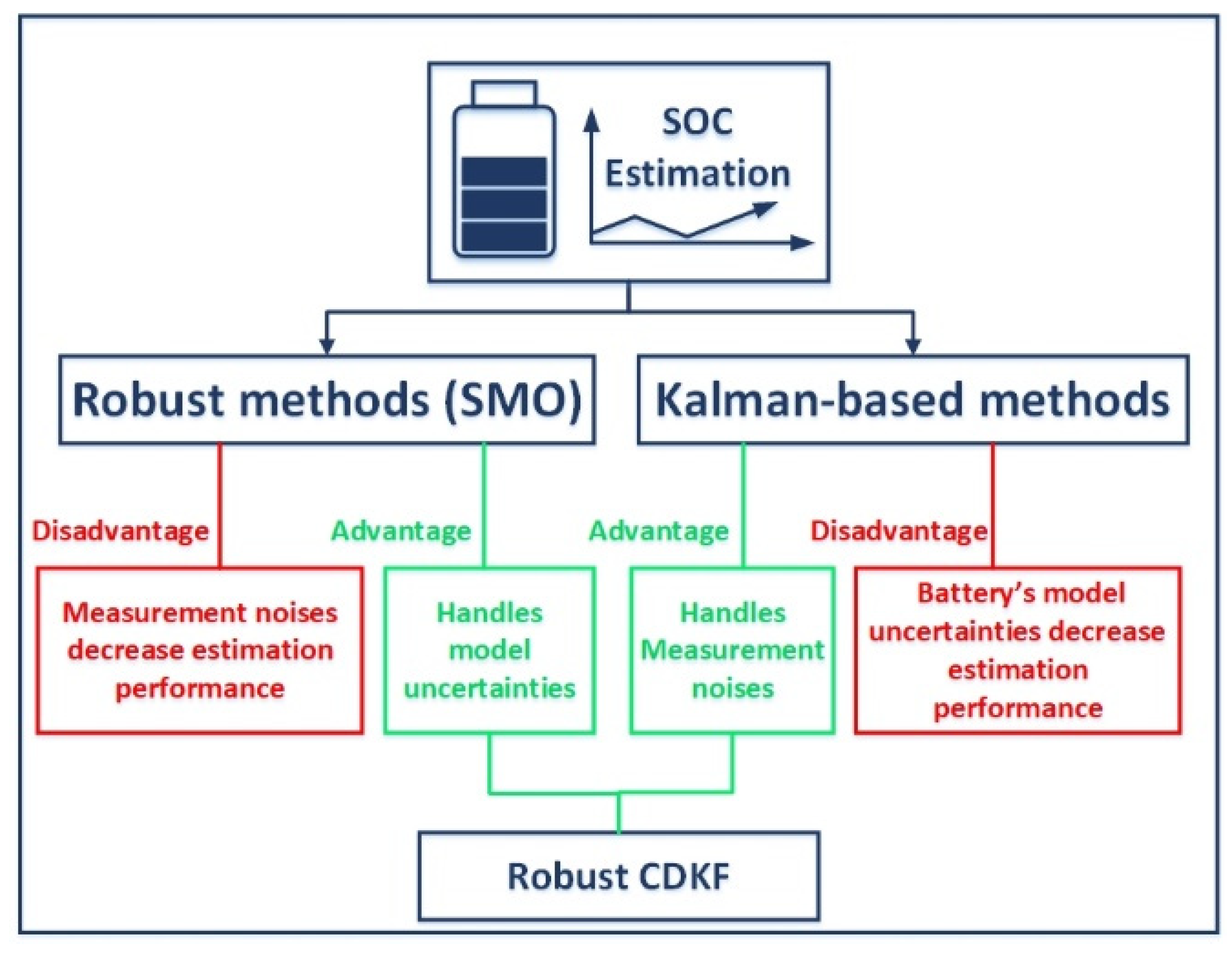
To tackle these problems, this paper introduces a robust CDKF for SoC estimation using an equivalent circuit model of batteries in the presence of the model uncertainty. The equivalent circuit model includes the capacitors, resistors, and nonlinear voltage source in order to show the nonlinear relation between the OCV and SoC. The main weakness of the conventional Kalman-based methods for SOC estimation is that they require an accurate model of the battery, while the robust methods can handle the battery model uncertainty. On the other hand, the main disadvantage of the sliding-mode-based methods is that the measurement and process noises affect their performance. This paper presents a new solution for these problems and uses the proposed robust CDKF to estimate the SOC in the presence of the model uncertainty and measurement noise simultaneously for on-site lithium-ion batteries in smart home applications. In addition, the proposed method can estimate SoC more accurately compared to the conventional CDKF. Figure 1 summarizes the robust methods, the Kalman-based methods, and the proposed CDKF method.

The rest of the paper is organized as follows: The dynamical model of the battery in the presence of uncertainties and noises is introduced in Section 2. Section 3 designs the proposed robust CDKF in order to estimate the SoC. In Section 4, the experimental tests for model identification of the battery and validation of the proposed method are presented. Finally, Section 5 concludes the paper.

2. Battery Modeling

There are diverse models for electrochemical batteries in various applications. These models can be classified into electrochemical, electrocircuit, and intelligent models in which the electrocircuit model is proper for the purpose of implementation of estimation algorithms such as SoC or SoH estimation.

The electrical model shown in Figure 2 is utilized in the proposed method [43]. There are several models for electrochemical batteries, such as electrochemical models, experimental models, electrical models, abstract models based on artificial intelligence, etc. Electrical models consist of several types, such as Thévenin models, Impedance models, Runtime-based models, and Randle equivalent-circuit models. The considered equivalent-circuit model for the battery is one of the most comprehensive electrical-based models. This model contains all the dynamic characteristics of the battery, including nonlinear open-circuit voltage, current, temperature, number of cycles, time-dependent storage capacity, and transient response. The usual Li-ion battery loss is represented by two resistances, $R_0$ and $R_{in}$. $R_0$ simulates the battery self-discharge and $R_{in}$ represents the battery losses related to the temperature changes, battery aging, and internal energy losses during the charging/discharging of the battery. This model anticipates all the important properties of the battery and is compatible with lead-acid batteries, nickel-cadmium, nickel-metal hybrids, ion batteries, lithium polymer, and other chemical batteries [43]. The variation of SoC during charging/discharging is simulated by the left side of the circuit, while the right side represents the transient response of the battery. Using the controlled voltage source $V_{oc}$, the nonlinear relation between SoC and OCV is simulated. Meanwhile, the series resistance denoted by $R_{in}$ is inserted to give the terminal voltage due to the load current $I_t$. Two series RC networks consisting of electrochemical polarization ($C_1$, $R_1$) and concentration polarization ($C_2$, $R_2$) simulate the short-term and long-term transient response of the battery at the relaxation effect, respectively. This relaxation effect is because of the double-layer charge/discharge or diffusion effect in the battery. $C_0$ and $R_0$ represent the whole charge capacitor and the self-discharge energy lost, respectively. According to the Kirchhoff laws, the terminal voltage can be written as follows:

$$V_t=V_{oc}(SoC)-V_1-V_2-I_t{R}_{in}$$

(2)

The dynamics of the state of charge and polarization voltages are as follows:

$$V_t=V_{oc}(SoC)-V_1-V_2-I_t{R}_{in}$$

(3)

$$\dot{S}oC=-\frac{1}{R_0{C}_0}SoC-(\frac{I_t}{C_0})+\Delta f_1$$

(4)

$${\dot{V}}_2=-\frac{V_2}{R_2{C}_2}+\frac{I_t}{C_2}+\Delta f_3$$

(5)

where $V_1$ and $V_2$ are electrochemical and concentrate voltages, respectively. $\Delta f_1$ to $\Delta f_4$ include the battery-model uncertainties and internal/external disturbances. Note that some of affecting factors, such as thermal effects, are considered in the model uncertainty. The experimental test for battery identification shows a nonlinear profile of V_oc vs. SoC. Using the curve-fitting method, this profile can be formulated as follows:

$$\begin{array}{l}{V}_{oc}(SoC)=G(SoC)\\ G(SoC)=3.35+1.29\hspace{0.17em}SoC-1.385\hspace{0.17em}So{C}^2\\ +0.826\hspace{0.17em}So{C}^3-3.97\hspace{0.17em}\exp (-38.3SoC)\end{array}$$

(6)

where $G(SoC)$ represents the nonlinear relation between the SoC and V_oc. Current It can be neglected, i.e., $d{I}_t/dt=0$. Substituting Equations (3)–(6) into Equation (2), the state equation of terminal voltage $V_t$ can be written as follows:

$$\begin{array}{l}{\dot{V}}_t=\frac{\partial V_{oc}}{\partial SoC}\dot{S}oC-{\dot{V}}_1-{\dot{V}}_2+\Delta f_4\\ \frac{\partial V_{oc}}{\partial SoC}=\dot{G}(SoC)\end{array}$$

(7)

where $\Delta f_4$ includes the uncertainty related to the inaccuracy of curve fitting. We define $X={[SoC,\hspace{0.17em}\hspace{0.17em}{V}_1,\hspace{0.17em}\hspace{0.17em}{V}_2,\hspace{0.17em}\hspace{0.17em}{V}_t]}^T$ as the state vector and assume the It and $V_t$ as the input and output of the battery, respectively. Based on Equations (3)–(5) and (7), the state space of the battery can be formulated as follows:

$$\begin{array}{l}\dot{X}=F(X,u)+\Delta f_{tot}+\zeta \hspace{0.17em}\hspace{0.17em}\hspace{0.17em}\hspace{0.17em}\hspace{0.17em}\hspace{0.17em}\hspace{0.17em}\hspace{0.17em}\hspace{0.17em}\hspace{0.17em}\hspace{0.17em}\hspace{0.17em}\hspace{0.17em}\hspace{0.17em}\zeta \approx (0,Q)\\ Y=CX\hspace{0.17em}\hspace{0.17em}+\hspace{0.17em}\omega \hspace{0.17em}\hspace{0.17em}\hspace{0.17em}\hspace{0.17em}\hspace{0.17em}\hspace{0.17em}\hspace{0.17em}\hspace{0.17em}\hspace{0.17em}\hspace{0.17em}\hspace{0.17em}\hspace{0.17em}\hspace{0.17em}\hspace{0.17em}\hspace{0.17em}\hspace{0.17em}\hspace{0.17em}\hspace{0.17em}\hspace{0.17em}\hspace{0.17em}\hspace{0.17em}\hspace{0.17em}\hspace{0.17em}\hspace{0.17em}\hspace{0.17em}\hspace{0.17em}\hspace{0.17em}\omega \approx (0,R)\\ C=[0\hspace{0.17em}\hspace{0.17em}\hspace{0.17em}0\hspace{0.17em}\hspace{0.17em}\hspace{0.17em}0\hspace{0.17em}\hspace{0.17em}\hspace{0.17em}1]\end{array}$$

(8)

where terms $\zeta ,\hspace{0.17em}\omega$ are the process and measurement noises with the zero mean. F and $\Delta f_{tot}$ can be expanded as

$$\begin{array}{l}F(X,\hspace{0.17em}u)=\left[\begin{array}{c}-\frac{1}{R_0{C}_0}SoC-(\frac{I_t}{C_0})\\ -\frac{V_1}{R_1{C}_1}+\frac{I_t}{C_1}\\ -\frac{V_2}{R_2{C}_2}+\frac{I_t}{C_2}\\ F_4(X,u)\end{array}\right]\\ F_4(X,u)=-\frac{1.29}{C_0}I+(\frac{-1.29}{R_0{C}_0}+\frac{2.77I}{C_0})SoC+(\frac{2.77}{R_0{C}_0}-\frac{2.478}{C_0}I)So{C}^2\\ +\frac{-2.478}{R_0{C}_0}So{C}^3-152.05(\frac{SoC}{R_0{C}_0}+\frac{I}{C_0})\exp (-38.3\hspace{0.17em}\hspace{0.17em}SoC)\end{array}$$

(9)

$$\Delta f_{tot}=\left[\begin{array}{c}\Delta f_1\\ \Delta f_2\\ \Delta f_3\\ \Delta f_4-\Delta f_2-\Delta f_3\end{array}\right]$$

(10)

According to Equation (8), the output equation is linear in terms of the $V_t$, which can be calculated from Equations (2) and (6).

3. Proposed Robust CDKF

According to the Equation (8), the discrete-time state-space equations of the battery are defined as follows:

$$\begin{array}{l}{\dot{X}}_i=F(X_{i-1},u)+\phi (X_{i-1})+{\zeta }_i\hspace{0.17em}\\ Y_i=h_t(X_i)\hspace{0.17em}+\gamma (X_i)\hspace{0.17em}+\hspace{0.17em}{\omega }_i\end{array}$$

(11)

${\zeta }_i$ and ${\omega }_i$ represent the process and measurement noises, respectively, and they have zero means and covariances as follows:

$$\begin{array}{l}E\hspace{0.17em}[{\zeta }_i\hspace{0.17em}{\zeta }_j^T]=Q_i{\psi }_{ij}\\ E\hspace{0.17em}[{\omega }_i\hspace{0.17em}{\omega }_j^T]=R_i{\psi }_{ij}\\ {\psi }_{ij}=\left\{\begin{array}{c}1,\hspace{0.17em}\hspace{0.17em}i=j\\ 0,\hspace{0.17em}\hspace{0.17em}i\ne j\end{array}\right.\end{array}$$

(12)

Note that $\phi (.)\hspace{0.17em},\hspace{0.17em}\gamma (.)$ are the bounded model uncertainties and their upper bounds can be derived by the information from the sensor.

$$\begin{array}{l}E[\phi (X_{i-1})\phi {(X_{i-1})}^T]\le \varphi {\varphi }^T\\ E[\gamma (X_i)\gamma {(X_i)}^T]\le \Gamma {\Gamma }^T\end{array}$$

(13)

Unlike the sigma-point Kalman filter or conventional CDKF, the proposed robust CDKF considers uncertainties in both state and output equations. Moreover, since the filtering methodology has been suggested based on the Stirling formula, it requires no derivative or Jacobian matrix computations. In addition, the proposed algorithm does not require the mean of uncertainties or any other special data associated with the statistical characteristics of uncertainties. For the lithium-ion battery, usually, there are model uncertainties caused by different issues, such as model identification errors, cell-to-cell variations, temperature variations, and measurement sensor errors. The uncertainties in both state and output equations cause inaccurate battery SoC estimation. The conventional sigma-point Kalman filter or conventional CDKF cannot cope with the uncertainty. To solve this problem, the proposed method—presented for the lithium-ion batteries for the first time—is a novel and practical choice. The step-by-step procedure of the proposed observer with a complete description of its equations is as follows:

Step 0: Initialization

Firstly, the initialization of the proposed observer must be performed.

$$\begin{array}{l}{\widehat{X}}_0=E(X_0)\\ {\widehat{P}}_{X_0}=E((X_0-{\widehat{X}}_0){(X_0-{\widehat{X}}_0)}^T)\end{array}$$

(14)

Step 1: Calculation of sigma points

Like the other sigma point Kalman filters, after selecting window size L and interval length d, sigma points are calculated as follows:

$${\eta }_{i-1}=\left[\begin{array}{ccc}{\widehat{X}}_{i-1}& {\widehat{X}}_{i-1}+d\sqrt{{\widehat{P}}_{i-1}}& {\widehat{X}}_{i-1}-d\sqrt{{\widehat{P}}_{i-1}}\end{array}\right]$$

(15)

where $\eta$ is the sigma-point vector and P is the covariance matrix of the estimation.

Step 2: Calculation of Weight coefficients

In this step, some of the weights are calculated to be able to calculate the state mean vector and the mean covariance matrix according to the propagated sigma points. The associated weights are derived as follows:

$$\begin{array}{l}{\upsilon }_0^{(m)}=\frac{d^2-L}{L},\hspace{0.17em}{\upsilon }_j^{(m)}=\frac{1}{2d^2}\hspace{0.17em}\hspace{0.17em},\hspace{0.17em}\hspace{0.17em}\hspace{0.17em}\hspace{0.17em}\hspace{0.17em}\hspace{0.17em}{\upsilon }_j^{(c1)}=\frac{1}{4d^2}\\ {\upsilon }_j^{(c2)}=\frac{(1+2{\lambda }^2)d^2-1}{4d^2}\end{array}$$

(16)

where n is the length of the state vector $(n=4)$.

Step 3: Propagation of sigma vectors

In this step, the calculated sigma points are propagated by inserting them into the nonlinear dynamics of the battery.

$${\eta }_{j,i|i-1}\hspace{0.17em}=F({\eta }_{j,i-1}\hspace{0.17em}\hspace{0.17em},u(k))$$

(17)

Step 4: Calculation of the state mean vector and the mean covariance matrix:

According to the propagated sigma vector, the state mean vector and the mean covariance matrix are calculated in Equations (18) and (19), respectively.

$${\widehat{X}}_{i|i-1}={\displaystyle \sum _{j=0}^{2n}{\upsilon }_j^{(m)}F({\eta }_{j,i-1})}$$

(18)

$$\begin{array}{l}{\widehat{P}}_{i|i-1}={\displaystyle \sum _{j=1}^n{\upsilon }_j^{(c1)}(F({\eta }_{j,i-1})-F({\eta }_{n+j,i-1})})\times (F({\eta }_{j,i-1})\\ -F({\eta }_{n+j,i-1}){)}^T+{\upsilon }_j^{(c2)}(F({\eta }_{j,i-1})+F({\eta }_{n+j,i-1})\\ -2F({\eta }_{0,i-1}))\times (F({\eta }_{j,i-1})+F({\eta }_{n+j,i-1})-\\ 2F({\eta }_{0,i-1}){)}^T+(1+{\lambda }^{-2})\varphi {\varphi }^T+Q_i\end{array}$$

(19)

where ${\widehat{X}}_{i|i-1}$, ${\widehat{P}}_{i|i-1}$, $\varphi {\varphi }^T$, and $Q_i$ are the state mean vector, mean covariance matrix, upper bound of the uncertainties in the state equations, and the process noise covariance matrix. One of the main improvements that are proposed by the robust CDKF is Equation (19), in which the model uncertainties in the state equations are considered. For the battery, these uncertainties are caused by different issues such as model identification errors, cell-to-cell variations, and temperature variations. According to this equation, this uncertainty problem is covered by the proposed observer.

Step 5: Propagation of the measurement equations

$${\eta }_{i|i-1}=\left[\begin{array}{ccc}{\widehat{X}}_{i|i-1}& {\widehat{X}}_{i|i-1}+d\sqrt{{\widehat{P}}_{i|i-1}}& {\widehat{X}}_{i|i-1}-d\sqrt{{\widehat{P}}_{i|i-1}}\end{array}\right]$$

(20)

By inserting the sigma points in Equation (20) into the output equation, the measurement equations are propagated as follows:

$${\widehat{Y}}_i={\displaystyle \sum _{j=0}^{2n}{\upsilon }_j^{(m)}h({\eta }_{j,i-1})}$$

(21)

Step 6: Calculation of the autocorrelation and cross-correlation matrices of the measurement:

The autocorrelation matrix is:

$$\begin{array}{l}{\widehat{P}}_Y={\displaystyle \sum _{j=1}^n{\upsilon }_j^{(c1)}(d({\eta }_{j,i|i-1})-d({\eta }_{n+j,i|i-1})})\times (d({\eta }_{j,i|i-1})\\ -d({\eta }_{n+j,i|i-1}){)}^T+{\upsilon }_j^{(c2)}(d({\eta }_{j,i|i-1})+d({\eta }_{n+j,i|i-1})\\ -2d({\eta }_{0,i|i-1}))\times (d({\eta }_{j,i|i-1})+d({\eta }_{n+j,i|i-1})-\\ 2d({\eta }_{0,i|i-1}){)}^T+(1+{\lambda }^{-2})\Gamma {\Gamma }^T+R_i\end{array}$$

(22)

The other improvement of the proposed method compared to a conventional SPKF is indicated in Equation (22). As shown in this equation, uncertainties in the output equations or measurements are considered in the calculation of the autocorrelation matrix in order to make the proposed observer robust against the output uncertainties. The cross-correlation matrix is calculated as follows:

$${\widehat{P}}_{XY}=\sqrt{{\upsilon }_1^{(c1)}{\widehat{P}}_{i|i-1}}{(d({\eta }_{1:n,i|i-1})-d({\eta }_{n+1:2n,i|i-1}))}^T$$

(23)

Step 7: Filter gain

In this step, the gain of the proposed filter, which corrects the prediction of the states in Step 4, is calculated as follows:

$$K_i={\widehat{P}}_{XY}{\widehat{P}}_Y{}^{-1}$$

(24)

Step 8: Updating the mean states vector and the mean covariance matrix

In the final step, the updated estimation of the battery’s state variables, including the SoC and the updated mean covariance matrix, is calculated as:

$${\widehat{X}}_i={\widehat{X}}_{i|i-1}+K_i(Y_i-{\widehat{Y}}_i)$$

(25)

$${\widehat{P}}_i={\widehat{P}}_{i|i-1}-K_i{\widehat{P}}_y{K}_i{}^T$$

(26)

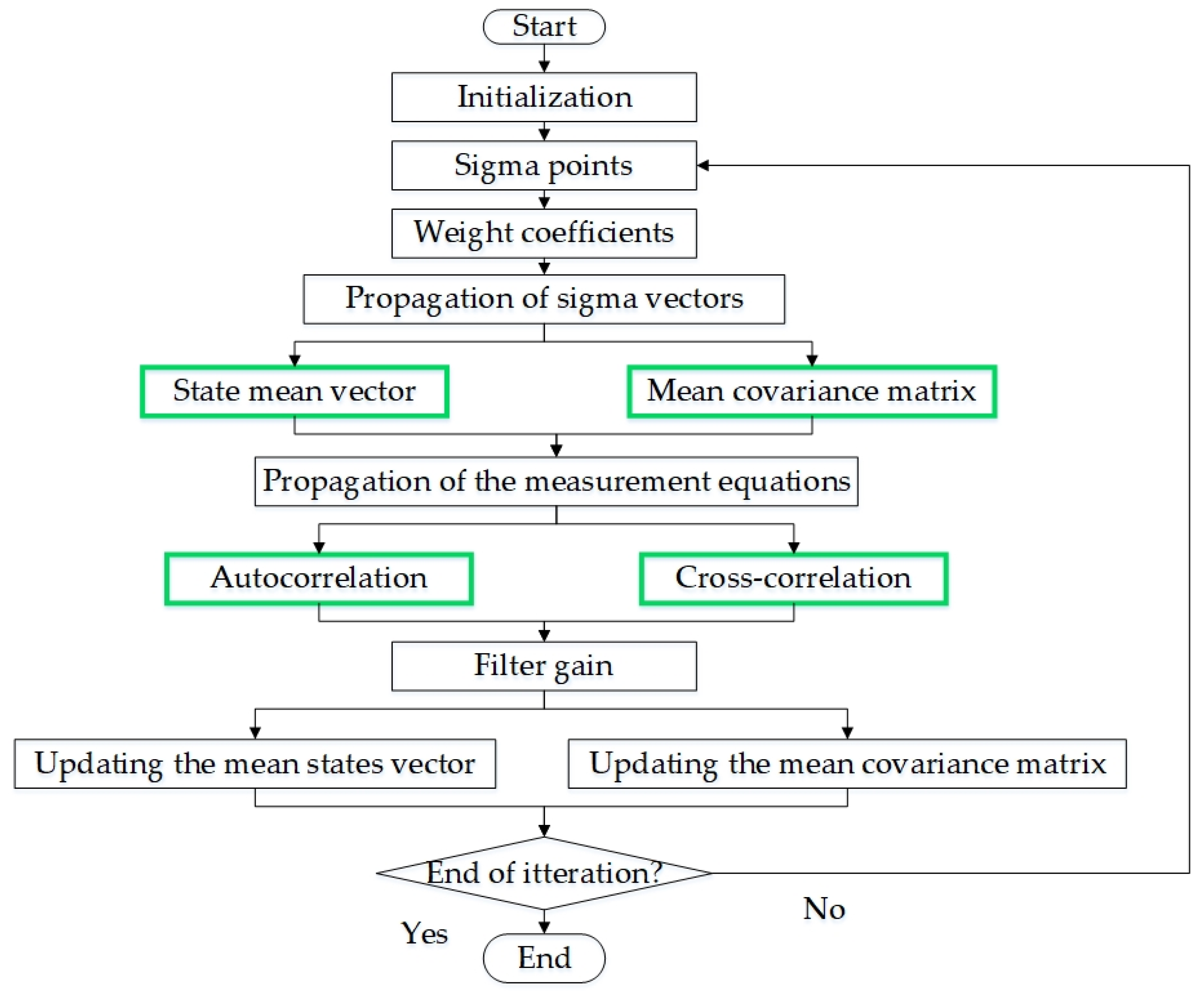
The steps of constructing the proposed method are summarized in the flowchart shown in Figure 3, where the steps with a green border indicate the main improvements of the proposed method.

4. Experimental Results

4.1. Test Setup

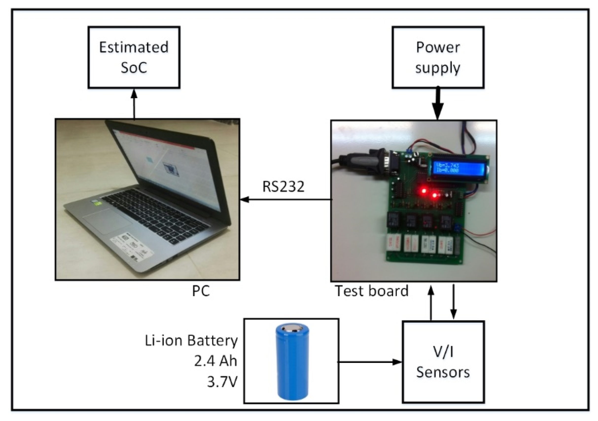
As shown in Figure 4, a test bench is assembled in order to identify and validate the battery model and also to verify the proposed SoC estimation method. In this paper, three common Li-ion batteries are used. The capacity is 2.4 Ah, and the nominal voltage is 3.7 V. The maximum and cut-off voltage are 4.1 V and 3 V, respectively. Some of the important characteristics of the battery cell have been collected in

Table A1. Some of the important characteristics of the battery cells.

Parameter	Value
Nominal Voltage	3.7 V
Discharge Cut-off Voltage	3.0 V
Max Charge Voltage	4.20 ± 0.05 V
Standard Charge Current	0.52 A
Rapid Charge Current	1.3 A
Standard Discharge Current	0.52 A
Rapid Discharge Current	1.3 A
Max Pulse Discharge Current	2.6 A
Weight	46.5 ± 1 g
Max. Dimension	Diameter (Ø): 18.4 mm Height (H): 65.2 mm
Operating Temperature	Charge: 0~45 °C Discharge: −20~60 °C
Storage Temperature	During 1 month: −5~35 °C During 6 months: 0~35 °C
Cathode	Metal oxide
Anode	Consists of porous carbon

in Appendix A. The main components on this test bench include a microcontroller, programmable resistive load, and a liquid crystal display (LCD). The microcontroller is used to control the load during the discharging of the battery. Internal 10-bit A/D converters are used to measure the currents and voltages with a sampling rate of 20 Hz. Using an RS232 serial port, the measured data are imported to a PC. These imported signals are used to identify and validate the battery model and SoC estimation. The LCD shows the SoC, voltages, and current.

4.2. Experimental Battery-Model Verification

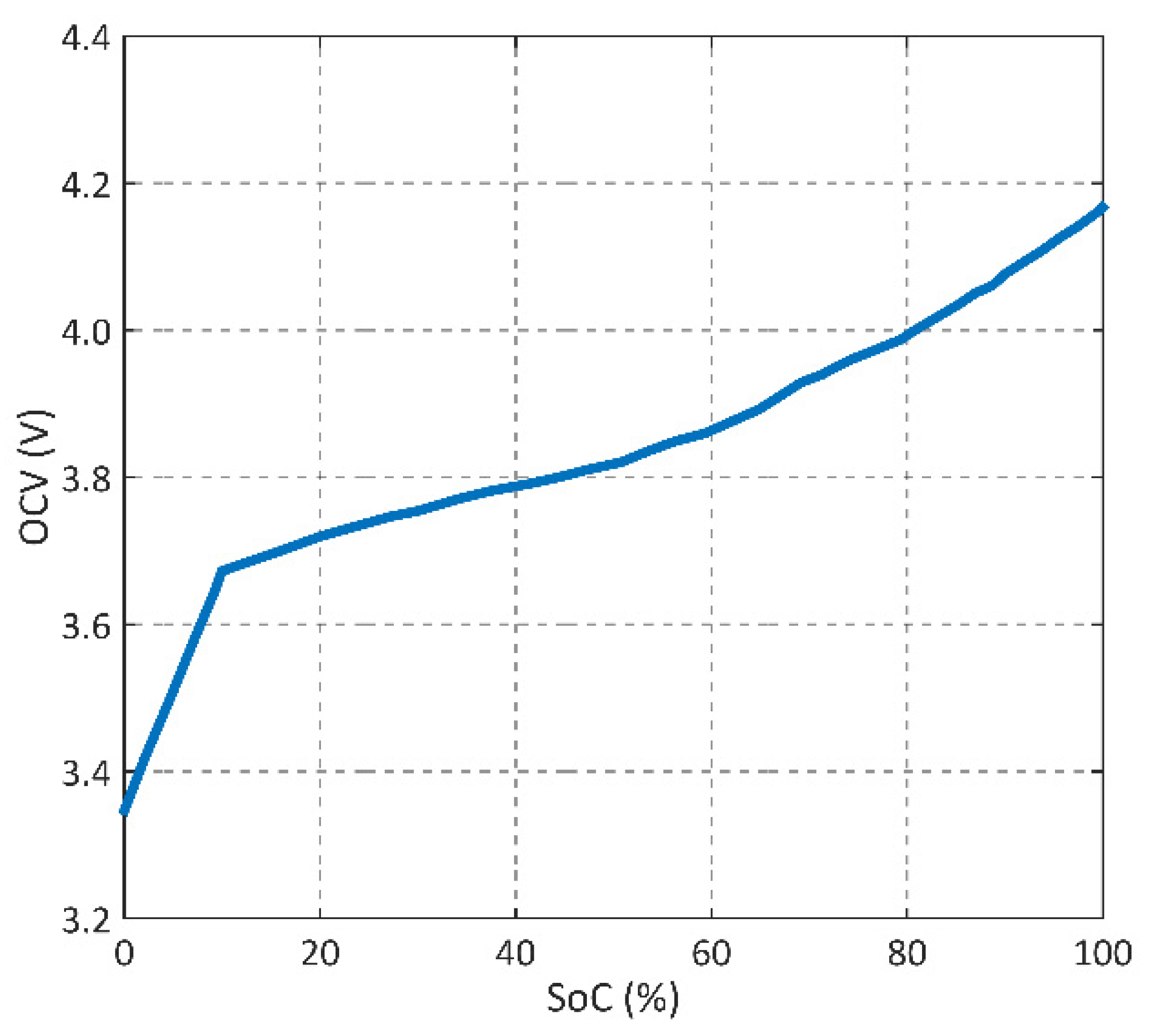
At room temperature, a resistive load is applied to the battery to discharge it from a fully charged level and measure the terminal voltage, OCV, and current during the discharging condition. An arbitrary current profile can be derived from the battery using a programmable load. In order to extract the OCV vs. SoC profile, the programmable resistive load discharged the battery at the rate of 0.7-C. This process continued until the terminal voltage received the value as much as the cut-off voltage of 3 V. This profile for the fresh battery cell is shown in Figure 5.

Based on the identification method presented in [17], the parameter values are extracted using the measured data.

Note that the $C_b$ is selected through the $C_b=3600\times {(capacity)}_{Ah}$. If the estimated SoC from the Ah counting method is consistent with the SoC obtained in Equation (3), the self-discharge resistor $R_{sd}$ can be extracted. Moreover, according to [17], $R_0$ is calculated using the ratio of the voltage variation to the current jump. As it is presented in this reference and using Equation (2), it follows that:

$$V_{oc}(Soc)-V_t-I_t{R}_{in}=V_{eq}$$

(27)

Considering $d{I}_t/dt=0$, the discrete form of Equation (27) is:

$$\begin{array}{l}{V}_{eq}(i)=(\frac{R_1(1-\exp (-T_s/T_{pf}))z^{-1}}{1-\exp (-T_s/T_{pf})z^{-1}}\\ +\frac{R_2(1-\exp (-T_s/T_{ps}))z^{-1}}{1-\exp (-T_s/T_{ps})z^{-1}})I_t(i)\\ =(\frac{z^{-1}(b_1+b_2{z}^{-1})}{1+a_1{z}^{-1}+a_2{z}^{-2}})I_t(i)\end{array}$$

(28)

where $T_s$ is the sampling period. $T_{pf}$ and $T_{ps}$ are the time constant of the RC networks. Using ARMAX method, the $a_1,\hspace{0.17em}{a}_2$ and $b_1,\hspace{0.17em}{b}_2$ can be calculated and so the RC networks parameters can be extracted from these factors.

Table 2. Battery cell #1 model parameters.

Parameter	Value
$R_0$ (Ω)	100
$R_{in}$ (m Ω)	88
$R_1$ (m Ω) $R_2$ (m Ω)	2.8 41.2
$C_0$ (F)	8640
$C_1$ (F) $C_2$ (F)	37 1376

shows the values of the model parameters estimated during the experimental validation.

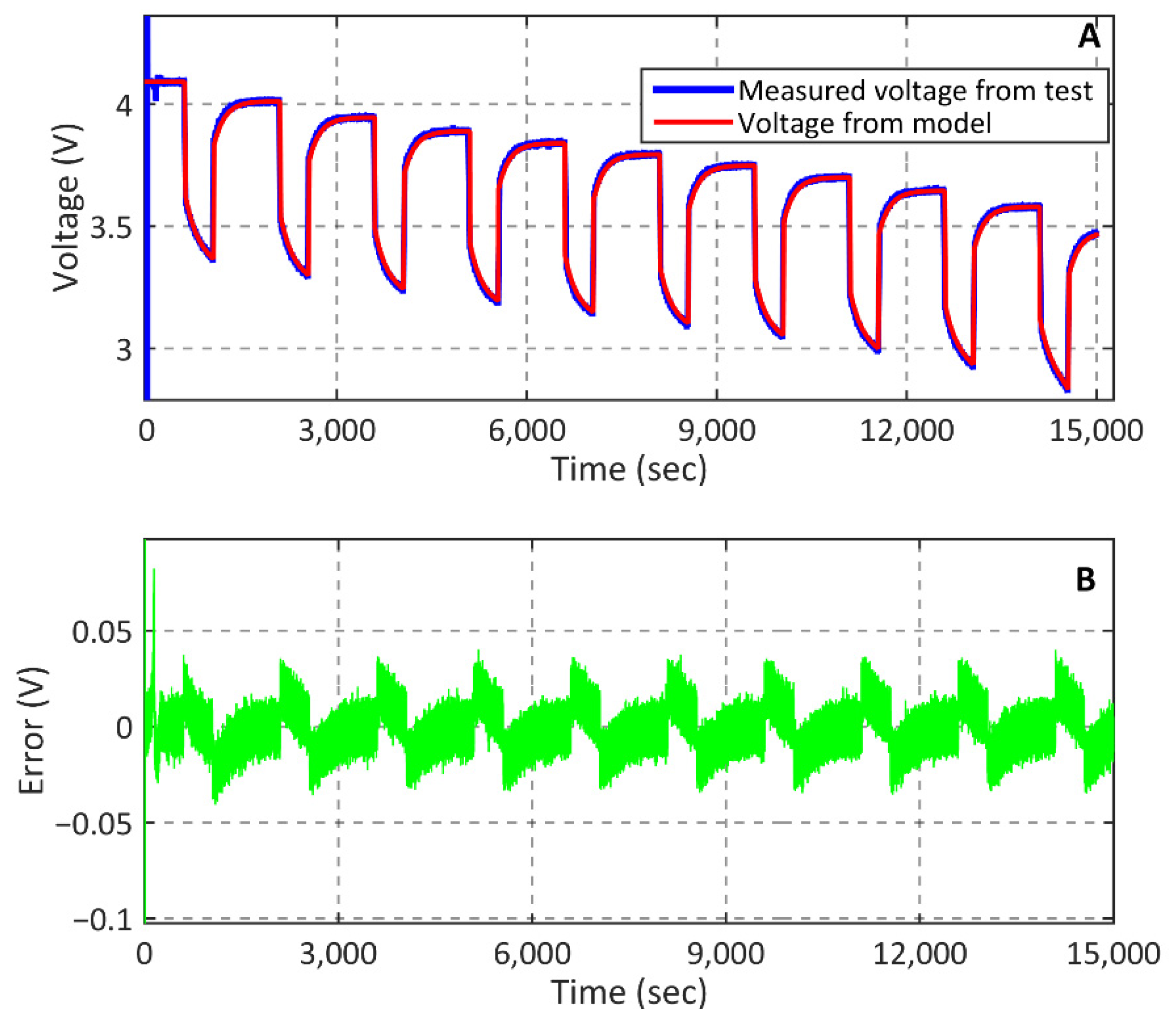
Note that the model parameters are identified at the room temperature and the thermal effects on these parameters are considered as the model uncertainty. Therefore, it can be found that the proposed robust method can cover the thermal effects on the accuracy of SoC estimation. Figure 6 shows the true voltage, model voltage, and the error of the modeling voltage during the experimental identification. The extracted voltage from the simulated model is close to the true value measured from the experiments. The maximum error of the voltage from the model compared to its true value is less than 50 mV and the average value of this error is −6.7 mV. In other words, the modeling error is about 1.2%, which is acceptable for the design of the proposed observer in comparison to other reported modeling errors in [11].

4.3. Robust CDKF Design

According to the model verification of the battery and its state-space equations in Equation (11), the dynamical model of the battery for the robust CDKF to implement on is given as

$$\begin{array}{l}{\dot{X}}_i=\left[\begin{array}{c}-(11.57\times {10}^{-7})\hspace{0.17em}\hspace{0.17em}SoC-(1.157\times {10}^{-4})\hspace{0.17em}\hspace{0.17em}{I}_t\\ -(9.65\times {10}^{-6})\hspace{0.17em}\hspace{0.17em}{V}_f+0.027I_t\\ -0.0176\hspace{0.17em}\hspace{0.17em}{V}_s+(7.26\times {10}^{-4})I_t\\ \begin{array}{l}(-28.7\times {10}^{-7})\hspace{0.17em}\hspace{0.17em}So{C}^3+((32.06\times {10}^{-7})-(2.86\times {10}^{-4})I)\hspace{0.17em}\hspace{0.17em}So{C}^2\\ +(32.06\times {10}^{-7})\hspace{0.17em}I.SoC-(I+1)(0.0176)\exp (-38.3\hspace{0.17em}\hspace{0.17em}SoC)\end{array}\end{array}\right]\\ \\ +\phi (X_{i-1})+{\zeta }_i\hspace{0.17em}\hspace{0.17em}\hspace{0.17em},\hspace{0.17em}\hspace{0.17em}\hspace{0.17em}{\zeta }_i\approx (0,Q_i)\\ \\ Y_i=(0\hspace{0.17em}\hspace{0.17em}\hspace{0.17em}0\hspace{0.17em}\hspace{0.17em}\hspace{0.17em}0\hspace{0.17em}\hspace{0.17em}\hspace{0.17em}1)X_i+\gamma (X_i)\hspace{0.17em}\hspace{0.17em}+\hspace{0.17em}{\omega }_i\hspace{0.17em}\hspace{0.17em}\hspace{0.17em}\hspace{0.17em}\hspace{0.17em}\hspace{0.17em},\hspace{0.17em}\hspace{0.17em}\hspace{0.17em}\hspace{0.17em}\hspace{0.17em}\hspace{0.17em}\hspace{0.17em}{\omega }_i\approx (0,R_i)\end{array}$$

(29)

Note that the measurement and model uncertainty of the battery are bounded as follows:

$$\begin{array}{l}E[\phi (X_{i-1})\phi {(X_{i-1})}^T]\le 1.5\times {10}^{-7}{I}_{4\times 4}\\ E[\gamma (X_i)\gamma {(X_i)}^T]\le 2.3\times {10}^{-13}\end{array}$$

(30)

$\lambda$ and the covariance matrix of the process and measurement noises are:

$$\begin{array}{l}Q={\sigma }_p{}^2{I}_{4\times 4}\hspace{0.17em}\hspace{0.17em}\hspace{0.17em}\hspace{0.17em}\hspace{0.17em},{\sigma }_p={10}^{-4}\\ R={\sigma }_m{}^{2}I\hspace{0.17em}\hspace{0.17em}\hspace{0.17em}\hspace{0.17em}\hspace{0.17em},{\sigma }_m=30\times {10}^{-4}\\ \lambda =0.0001\end{array}$$

(31)

4.4. Verification of the Proposed Estimator

In order to validate the performance of the proposed robust CDKF, especially its robustness, the experimental tests were carried out for a fresh and an aged battery. The aged battery was tested in order to show the robustness of the proposed, in a case in which the model uncertainty of the battery is changed.

4.4.1. Experimental Tests for the Fresh Battery

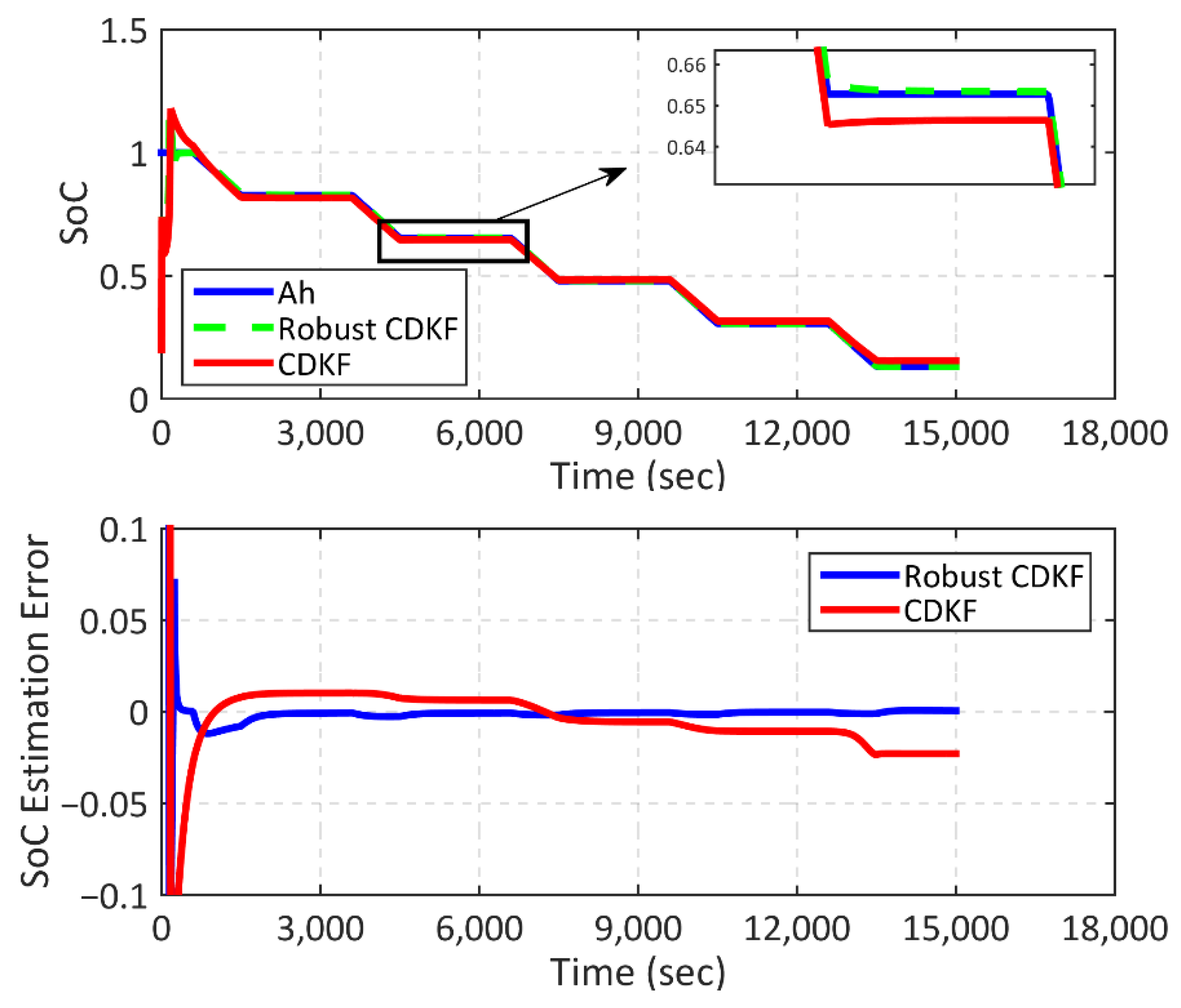
In this case, the fresh battery was discharged using a programmable load that causes a pulse-discharging current with amplitude, pulse period, and pulse width of 5 A, 500 s, and 30%, respectively. The proposed SoC estimation method is compared to the central-difference Kalman filter in order to show the effectiveness of the proposed method, especially in the presence of the model uncertainty.

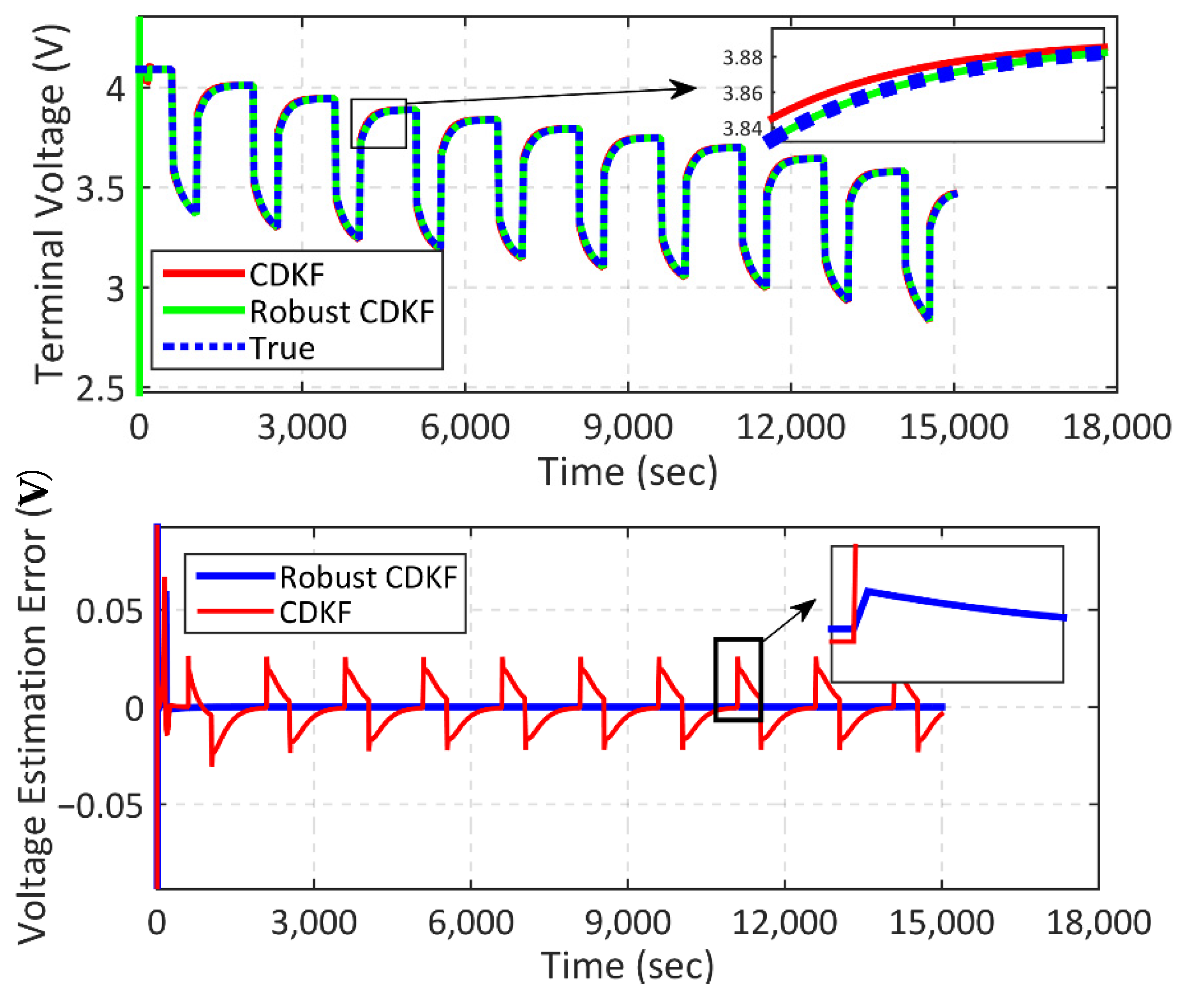
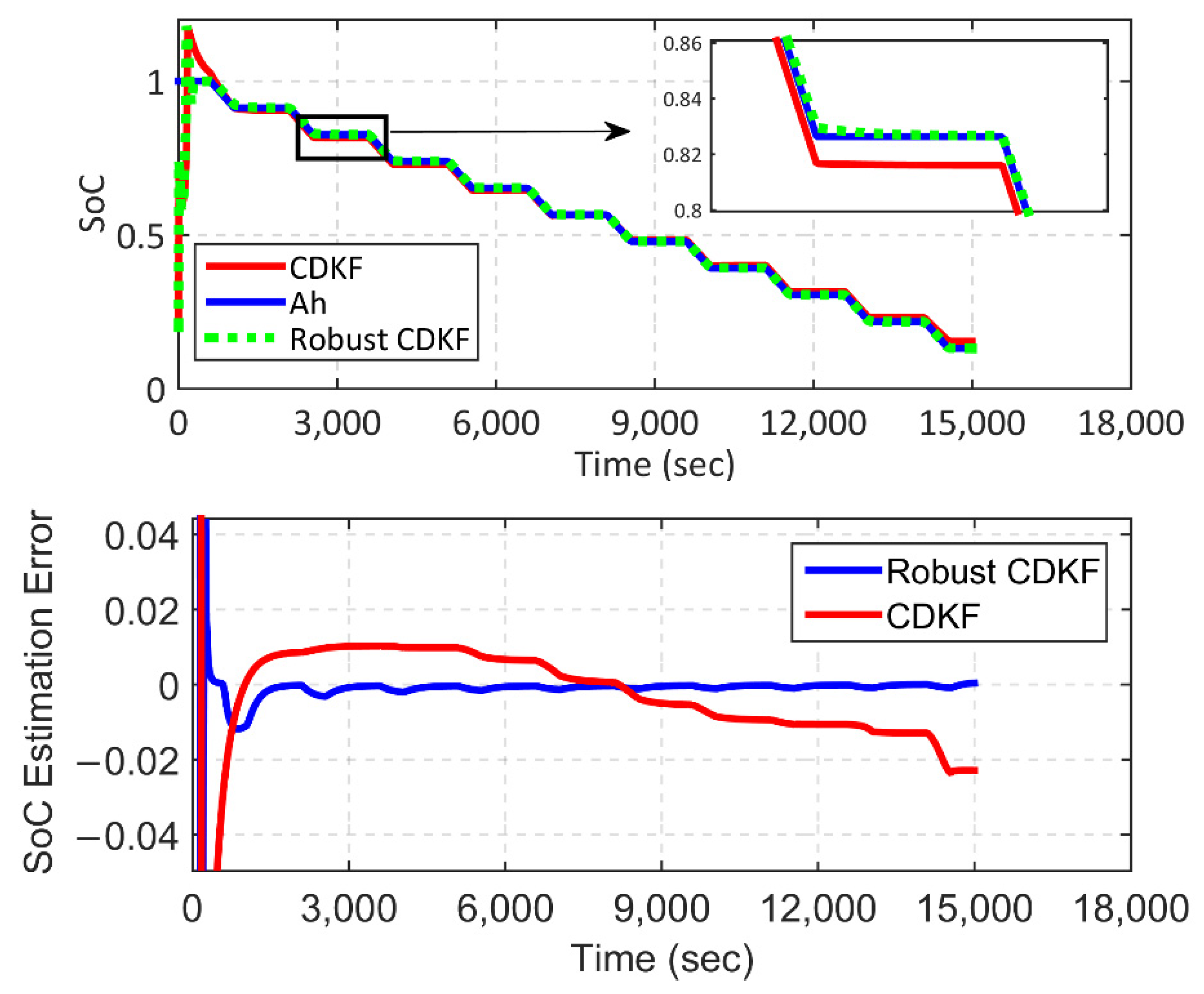
The estimation of the terminal voltage and SoC are shown in Figure 7 and Figure 8. According to Figure 8, the estimated terminal voltage using the robust CDKF method follows the true value with a tracking error of 1.3 mV. As it is shown in Figure 8, compared to the Ah method, the SoC is estimated using the robust CDKF method with an error of 0.1% in most times of discharge. As the model identification of the battery is not absolutely accurate, the CDKF cannot withstand the model uncertainties. By contrast, the proposed robust CDKF can estimate the estate variables, including the SoC and terminal voltage, in the presence of the model uncertainties. The experimental results show that the proposed robust CDKF is much more accurate than the CDKF method in SoC estimation. More specifically, as shown in Figure 7, the estimated terminal voltage using the robust CDKF has less error as much as 0.0183 V compared to the CDKF method. Figure 8 also confirms that the SoC estimation using the proposed method is more accurate than the CDKF. According to this figure, the estimated SoC using CDKF has a 0.9% higher error than the proposed method.

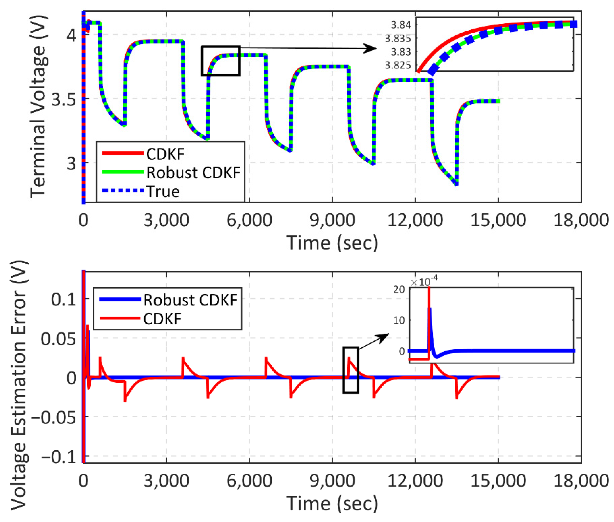
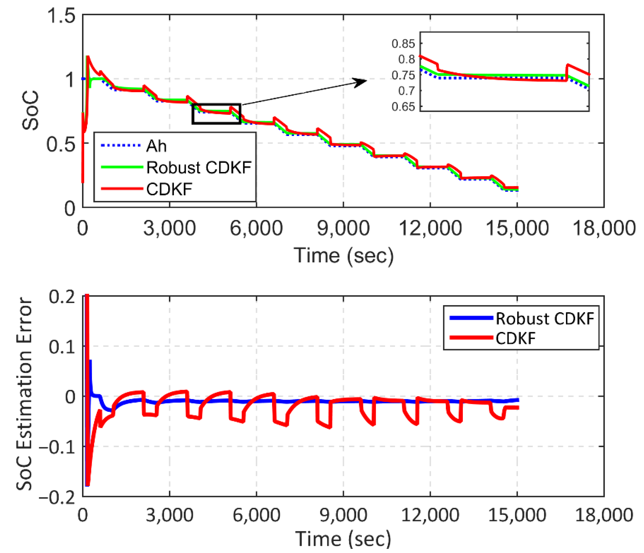
In order to validate the performance of the robust CDKF for another battery current with a lower frequency (The time period of 1000 s), the experimental tests were carried out in another discharging case in which the programmable load was rearranged so that the required pulse current was extracted from the battery. In this case, the performance of the proposed method was compared to the performance of the CDKF in Figure 9 and Figure 10. Using the proposed robust CDKF, the estimation of the SoC and terminal voltage is more accurate than the CDKF. Specifically, the estimation error of the SoC and terminal voltage using the typical CDKF are 0.9% and 0.024 V higher than using the proposed robust method.

4.4.2. Experimental Tests for the Aged Battery

For the SoC estimation, the model of a fresh battery is usually used. However, after a long time operating the battery, the aging problem makes some changes in its model parameters. The model-based SoC estimator, designed based on the fresh battery model, will not have acceptable performance, and the SoC estimation error will increase. In order to validate the robust performance of the proposed robust CDKF for the aging problem, a set of experiments were carried out for an aged battery. In Figure 11 and Figure 12, the performance of the proposed method in estimating the terminal voltage and SoC for the aged battery is compared to the performance of the conventional CDKF. As shown in Figure 7 and Figure 11, the estimation accuracy of the terminal voltage using the robust CDKF for the aged battery is lower than its performance for the fresh battery. However, this accuracy reduction is very low compared to the performance of the CDKF for the fresh and aged battery. In other words, the aging issue significantly affects the performance of the CDKF. Specifically, the accuracy of the terminal voltage estimation decreases by 8 mV compared to its performance for the fresh battery. The aging issue increases the model uncertainty of the battery, which weakens the performance of the conventional CDKF. However, the proposed method can cope with this model uncertainty.

Table 3. Comparison of the SoC estimation errors for Cells #1, 2, and 3.

Fresh/Aged	Method	SoC Estimation	Terminal Voltage Estimation
Fresh battery	Robust CDKF (500 s)	0.1%	~0 V
	CDKF (500 s)	2%	0.05 V (pick to pik)
	Robust CDKF (1000 s)	0.1%	~0 V
	CDKF (1000 s)	2%	0.04 V (pick to pik)
Aged battery	Robust CDKF	1%	0.001 V
	CDKF	5%	0.1 V (pick to pik)

summarizes the results of the SoC and terminal voltage estimation for the fresh and aged batteries using the proposed robust RCDKF and conventional CDKF.

4.4.3. Experimental Tests for Cell-to-Cell and Temperature Variations

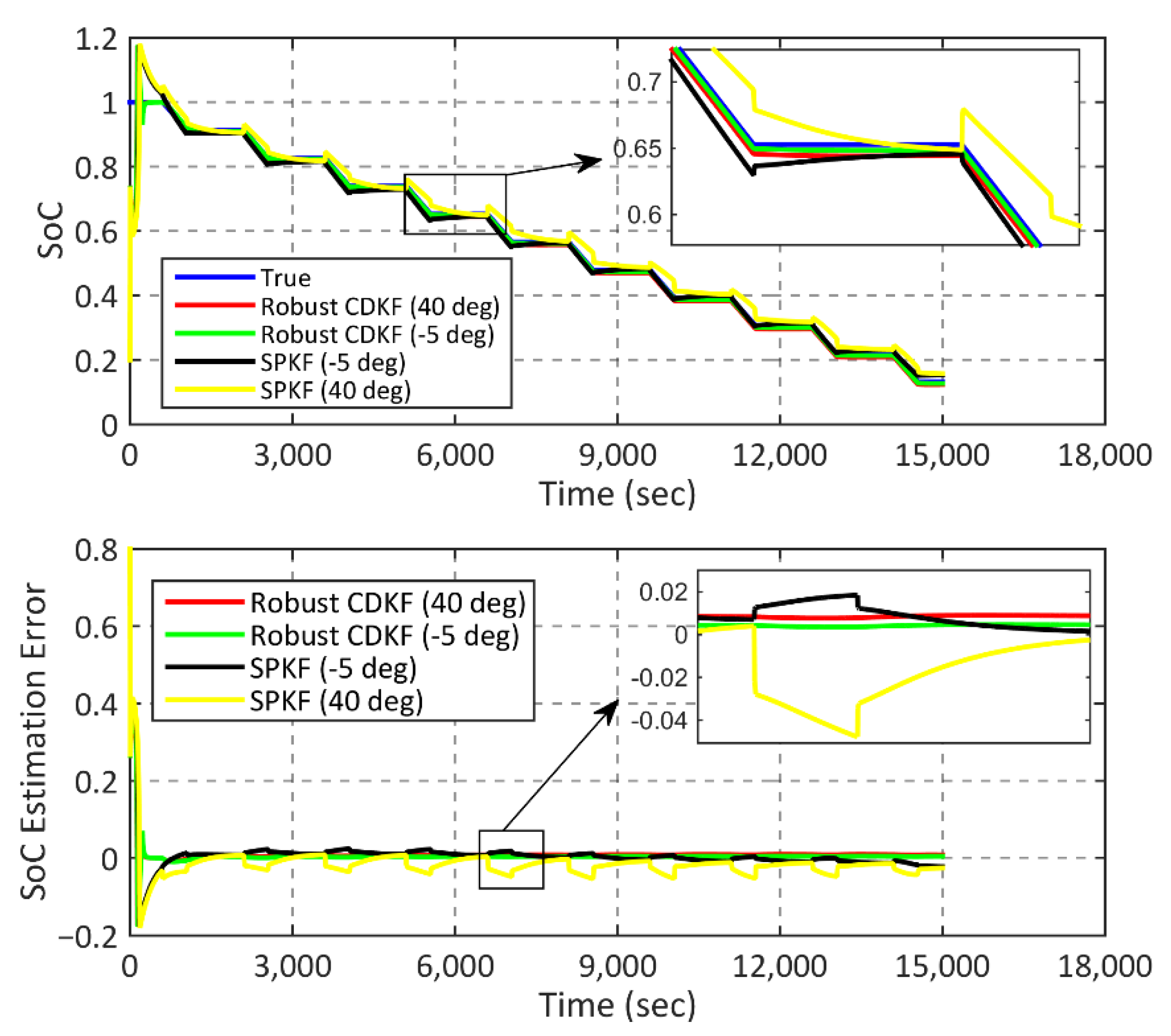
A set of experiments were carried out on two other battery cells (cell #2 and #3) at two different temperatures (−5 and 40 degrees), and the performance of the proposed method was compared to the performance of a sigma-point Kalman filter (SPKF). The model parameters of two fresh and similar battery cells are identified and shown in

Table 4. Battery cell #2 model parameters.

Parameter	Value
$R_0$ (Ω)	109
$R_{in}$ (m Ω)	86
$R_1$ (m Ω) $R_2$ (m Ω)	2.4 43.4
$C_0$ (F)	8640
$C_1$ (F) $C_2$ (F)	35 1377

and

Table 5. Battery cell #3 model parameters.

Parameter	Value
$R_0$ (Ω)	98
$R_{in}$ (m Ω)	89
$R_1$ (m Ω) $R_2$ (m Ω)	2.1 40
$C_0$ (F)	8640
$C_1$ (F) $C_2$ (F)	39 1379

.

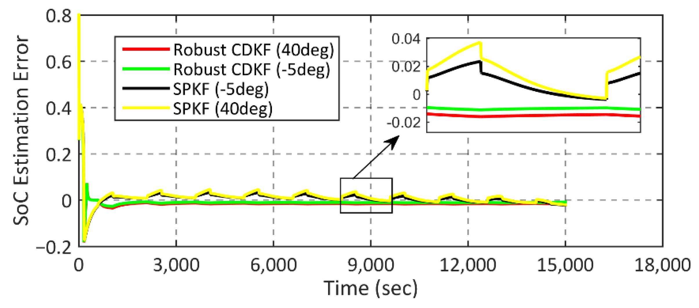
Figure 13 shows the experimental results of cell #2. The SPKF method has errors of 2.5% and 5% at temperatures of −5 and 40 degrees, respectively. By contrast, the proposed robust CDKF has estimation errors of 0.5% and 1% at temperatures of −5 and 40 degrees, respectively.

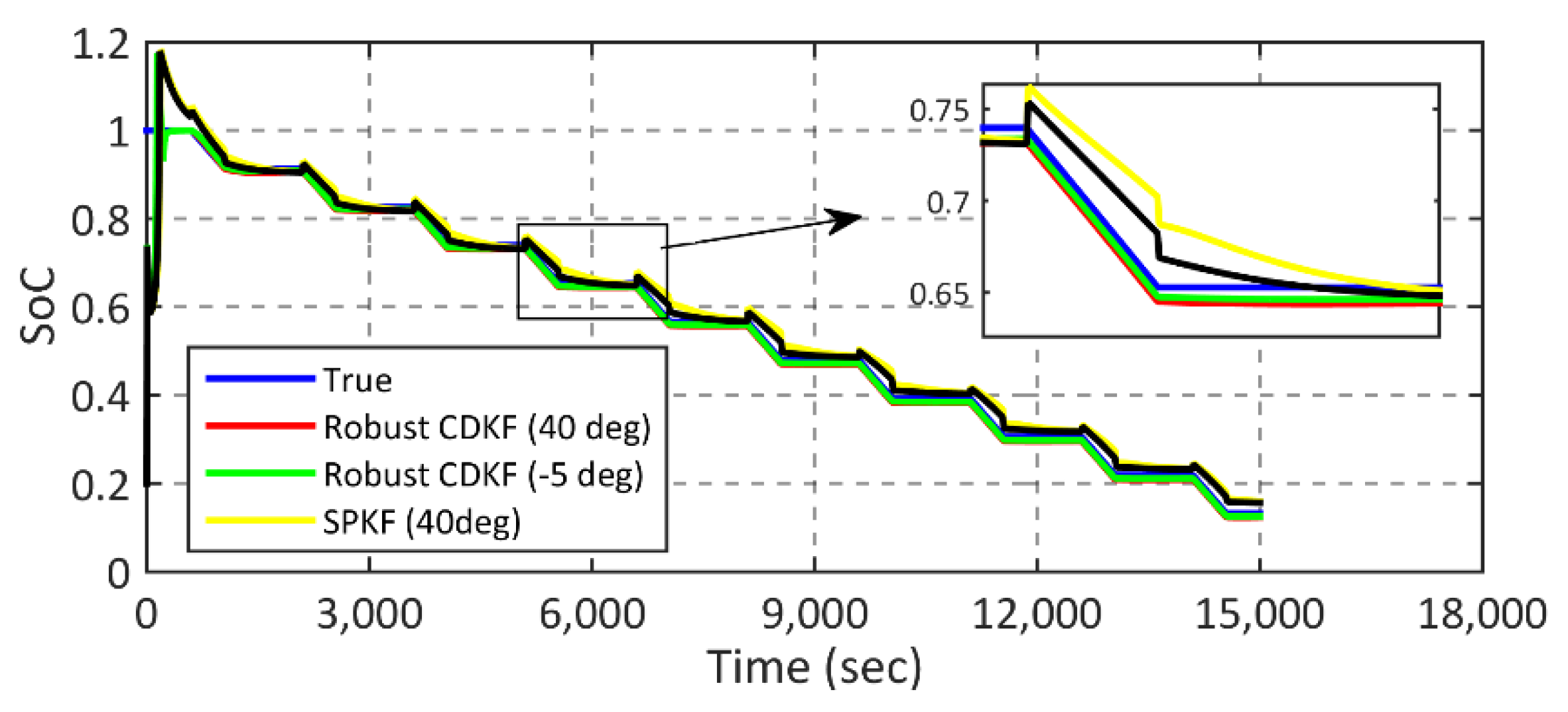
Figure 14 shows the experimental results of cell #3, which are different from battery cell #2 due to the cell-to-cell variations. The SPKF has errors of 3% and 4% at temperatures of −5 and 40 degrees, respectively. By contrast, the proposed method has errors of 0.7% and 1.1%, respectively.

Table 6. Comparison of the SoC estimation errors for cells #1, 2, and 3.

	Robust CDKF	SPKF	CDKF
Cell #1—Fresh (Room temp)	0.1%	-	2%
Cell #1—Aged (Room temp)	1%		5%
Cell #2 (−5 deg)	0.5%	2.5%	-
Cell #2 (40 deg)	1%	5%	-
Cell #3 (−5 deg)	0.7%	3%	-
Cell #3 (40 deg)	1.1%	4%	-

summarizes the experimental results. As can be seen, the model uncertainty caused by variations of different cells and temperatures will increase the SoC estimation error in both robust CDKF and SPKF methods. The SPKF method does not consider the model uncertainty in its algorithm and is not robust to variations. By contrast, the proposed robust CDKF performs better with much lower errors. In other words, the proposed method is robust against the model uncertainties.

5. Conclusions

In this paper, a Robust CDKF approach is proposed for SoC estimation for the lithium-ion battery. The proposed method uses the equivalent circuit model of the battery in the presence of the model uncertainty. The main advantage of this method compared to other Kalman filter-based methods is its robust behavior in the presence of the model uncertainty and measurement noise. In addition, the proposed method can overcome the limitation of the classic observers, such as sliding-mode observers against the process and measurement noises. Moreover, after a long period of operation of the batteries, the model uncertainties will increase, weakening the performance of the other Kalman-based methods, which require an accurate battery model. In contrast, the proposed robust method can withstand the uncertainties that occur with the aging problem. The experimental results show the feasibility and effectiveness of the proposed algorithm for both fresh and aged batteries as well as its superiority over the CDKF method.

References

- Zubi, G.; Dufo-López, R.; Pardo, N.; Pasaoglu, G. Concept development and techno-economic assessment for a solar home system using lithium-ion battery for developing regions to provide electricity for lighting and electronic devices. Energy Convers. Manag. 2016, 122, 439–448. [Google Scholar] [CrossRef]
- Piller, S.; Perrin, M.; Jossen, A. Methods for state-of-charge determination and their applications. J. Power Sources 2001, 96, 113–120. [Google Scholar] [CrossRef]
- Rezaei, O.; Alinejad, M.; Nejati, S.A.; Chong, B. An optimized adaptive estimation of state of charge for Lithium-ion battery based on sliding mode observer for electric vehicle application. In Proceedings of the 2020 8th International Conference on Intelligent and Advanced Systems (ICIAS), Kuching, Malaysia, 13–15 July 2021; pp. 1–6. [Google Scholar]
- Pei, L.; Lu, R.; Zhu, C. Relaxation model of the open-circuit voltage for state-of-charge estimation in lithium-ion batteries. IET Electr. Syst. Transp. 2013, 3, 112–117. [Google Scholar] [CrossRef]
- Cheng, M.W.; Lee, Y.S.; Liu, M.; Sun, C.C. State-of-charge estimation with aging effect and correction for lithium-ion battery. IET Electr. Syst. Transp. 2015, 5, 70–76. [Google Scholar] [CrossRef]
- Espedal, I.B.; Jinasena, A.; Burheim, O.S.; Lamb, J.J. Current trends for state-of-charge (SoC) estimation in lithium-ion battery electric vehicles. Energies 2021, 14, 3284. [Google Scholar] [CrossRef]
- Cuadras, A.; Kanoun, O. SoC Li-ion battery monitoring with impedance spectroscopy. In Proceedings of the 6th IEEE International Multi-Conference on Systems, Signals and Device, Djerba, Tunisia, 23–26 March 2009; Volume 5, pp. 1–5. [Google Scholar]
- Gholizadeh, M.; Yazdizadeh, A. State of charge estimation of a lithium-ion battery using robust nonlinear observer approach. IET Electr. Syst. Transp. 2018, 9, 1–7. [Google Scholar] [CrossRef]
- Zhang, Z.; Zhou, D.; Xiong, N.; Zhu, Q. Non-fragile H∞ nonlinear observer for state of charge estimation of lithium-ion battery based on a fractional-order model. Energies 2021, 14, 4771. [Google Scholar] [CrossRef]
- Ebrahimi, F.; Abedi, M. Design of a robust central difference Kalman filter in the presence of uncertainties and unknown measurement errors. Signal Process. 2020, 172, 107533. [Google Scholar] [CrossRef]
- Yao, J.; Ding, J.; Cheng, Y.; Feng, L. Sliding mode-based H-infinity filter for SOC estimation of lithium-ion batteries. Ionics 2021, 27, 5147–5157. [Google Scholar] [CrossRef]
- Chen, N.; Zhang, P.; Dai, J.; Gui, W. Estimating the state-of-charge of lithium-ion battery using an H-infinity observer based on electrochemical impedance model. IEEE Access 2020, 8, 26872–26884. [Google Scholar] [CrossRef]
- Verbrugge, M.; Tate, E. Adaptive state of charge algorithm for nickel metal hydride batteries including hysteresis phenomena. J. Power Sources 2004, 126, 236–249. [Google Scholar] [CrossRef]
- Chen, Z.; Sun, H.; Dong, G.; Wei, J.; Wu, J.I. Particle filter-based state-of-charge estimation and remaining-dischargeable-time prediction method for lithiumion batteries. J. Power Source 2019, 414, 158–166. [Google Scholar] [CrossRef]
- Xia, B.; Chen, C.; Tian, Y.; Sun, W.; Xu, Z.; Zheng, W. A novel method for state of charge estimation of lithium-ion batteries using a nonlinear observer. J. Power Sources 2014, 270, 359–366. [Google Scholar] [CrossRef]
- Hu, Y.; Yurkovich, S. Battery cell state-of-charge estimation using linear parameter varying system techniques. J. Power Sources 2012, 198, 338–350. [Google Scholar] [CrossRef]
- Gholizadeh, M.; Salmasi, F.R. Estimation of state of charge, unknown nonlinearities, and state of health of a lithium-ion battery based on a comprehensive unobservable model. IEEE Trans. Ind. Electron. 2013, 61, 1335–1344. [Google Scholar] [CrossRef]
- Rezaei, O.; Moghaddam, H.A.; Papari, B. A fast sliding-mode-based estimation of state-of-charge for lithium-ion batteries for electric vehicle applications. J. Energy Storage 2022, 45, 103484. [Google Scholar] [CrossRef]
- Zhong, Q.; Zhong, F.; Cheng, J.; Li, H.; Zhong, S. State of charge estimation of lithium-ion batteries using fractional order sliding mode observer. ISA Trans. 2017, 66, 448–459. [Google Scholar] [CrossRef] [PubMed]
- Chen, X.; Shen, W.; Cao, Z.; Kapoor, A. A novel approach for state of charge estimation based on adaptive switching gain sliding mode observer in electric vehicles. J. Power Sources 2014, 246, 667–678. [Google Scholar] [CrossRef]
- Chan, C.C.; Lo, E.W.C.; Shen, W. The available capacity computation model based on artificial neural network for lead–acid batteries in electric vehicles. J. Power Sources 2000, 87, 201–204. [Google Scholar] [CrossRef]
- Shen, W.X.; Chan, C.C.; Lo, E.W.C.; Chau, K.T. A new battery available capacity indicator for electric vehicles using neural network. Energy Convers. Manag. 2002, 43, 817–826. [Google Scholar] [CrossRef]
- Yang, F.; Li, W.; Li, C.; Miao, Q. State-of-charge estimation of lithium-ion batteries based on gated recurrent neural network. Energy 2019, 175, 66–75. [Google Scholar] [CrossRef]
- Habibifar, R.; Karimi, M.R.; Ranjbar, H.; Ehsan, M. Economically based distributed battery energy storage systems planning in microgrids. In Proceedings of the Iranian Conference on Electrical Engineering (ICEE), Mashhad, Iran, 8–10 May 2018; pp. 1257–1263. [Google Scholar]
- Charkhgard, M.; Farrokhi, M. State-of-charge estimation for lithium-ion batteries using neural networks and EKF. IEEE Trans. Ind. Electron. 2010, 57, 4178–4187. [Google Scholar] [CrossRef]
- Xu, P.; Liu, B.; Hu, X.; Ouyang, T.; Chen, N. State-of-charge estimation for lithium-ion batteries based on fuzzy information granulation and asymmetric Gaussian membership function. IEEE Trans. Ind. Electron. 2021, 69, 6635–6644. [Google Scholar] [CrossRef]
- Huang, Z.; Fang, Y.; Xu, J. SoC estimation of li-ion battery based on improved EKF algorithm. Int. J. Automot. Technol. 2021, 22, 335–340. [Google Scholar] [CrossRef]
- Hannan, M.A.; How, D.N.; Lipu, M.S.; Mansor, M.; Ker, P.J.; Dong, Z.Y.; Sahari, K.S.M.; Tiong, S.K.; Muttaqi, K.M.; Mahlia, T.M.; et al. Deep learning approach towards accurate state of charge estimation for lithium-ion batteries using self-supervised transformer model. Sci. Rep. 2021, 11, 1–13. [Google Scholar] [CrossRef]
- Lipu, M.S.H.; Hannan, M.A.; Hussain, A.; Saad, M.H.; Ayob, A.; Uddin, M.N. Extreme learning machine model for state-of-charge estimation of lithium-ion battery using gravitational search algorithm. IEEE Trans. Ind. Appl. 2019, 55, 4225–4234. [Google Scholar] [CrossRef]
- Chemali, E.; Kollmeyer, P.J.; Preindl, M.; Emadi, A. State-of-charge estimation of Li-ion batteries using deep neural networks: A machine learning approach. J. Power Sources 2018, 400, 242–255. [Google Scholar] [CrossRef]
- Yang, K.; Tang, Y.; Zhang, S.; Zhang, Z. A deep learning approach to state of charge estimation of lithium-ion batteries based on dual-stage attention mechanism. Energy 2022, 244, 123233. [Google Scholar] [CrossRef]
- Bian, C.; Yang, S.; Miao, Q. Cross-domain state-of-charge estimation of Li-ion batteries based on deep transfer neural network with multiscale distribution adaptation. IEEE Trans. Transp. Electrif. 2020, 7, 1260–1270. [Google Scholar] [CrossRef]
- Li, W.; Yang, Y.; Wang, D.; Yin, S. The multi-innovation extended Kalman filter algorithm for battery SOC estimation. Ionics 2020, 26, 6145–6156. [Google Scholar] [CrossRef]
- Malysz, P.; Gu, R.; Ye, J.; Yang, H.; Emadi, A. State-of-charge and state-of-health estimation with state constraints and current sensor bias correction for electrified powertrain vehicle batteries. IET Electr. Syst. Transp. 2016, 6, 136–144. [Google Scholar] [CrossRef]
- Gholizadeh, M.; Yazdizadeh, A. Systematic mixed adaptive observer and EKF approach to estimate SOC and SOH of lithium–ion battery. IET Electr. Syst. Transp. 2019, 10, 135–143. [Google Scholar] [CrossRef]
- Kim, J.; Cho, B.H. State-of-charge estimation and state-of-health prediction of a Li-ion degraded battery based on an EKF combined with a per-unit system. IEEE Trans. Veh. Technol. 2011, 60, 4249–4260. [Google Scholar] [CrossRef]
- Xiong, R.; He, H.; Sun, F.; Zhao, K. Evaluation on state of charge estimation of batteries with adaptive extended Kalman filter by experiment approach. IEEE Trans. Veh. Technol. 2012, 62, 108–117. [Google Scholar] [CrossRef]
- Li, J.; Ye, M.; Gao, K.; Jiao, S.; Xu, X. A novel battery state estimation model based on unscented Kalman filter. Ionics 2021, 27, 2673–2683. [Google Scholar] [CrossRef]
- Sun, F.; Hu, X.; Zou, Y.; Li, S. Adaptive unscented Kalman filtering for state of charge estimation of a lithium-ion battery for electric vehicles. Energy 2011, 36, 3531–3540. [Google Scholar] [CrossRef]
- Plett, G. Sigma-point Kalman filtering for battery management systems of LIPB-based HEV battery packs: Part 2: Simultaneous state and parameter estimation. J. Power Source 2006, 161, 1369–1384. [Google Scholar] [CrossRef]
- Sangwan, V.; Kumar, R.; Rathore, A.K. State-of-charge estimation for Li-ion battery using extended Kalman filter (EKF) and central difference Kalman filter (CDKF). In Proceedings of the 2017 IEEE Industry Applications Society Annual Meeting, Cincinnati, OH, USA, 1–5 October 2017; pp. 1–6. [Google Scholar]
- Chen, D.; Wang, C.; Zhu, Z.; Zou, Z. Lithium battery state-of-charge estimation based on interactive multi-model unscented Kalman filter Algorithm. Energy Storage Sci. Technol. 2020, 9, 257. [Google Scholar]
- Chen, M.; Rincon-Mora, G.A. Accurate electrical battery model capable of predicting runtime and IV performance. IEEE Trans. Energy Convers. 2006, 21, 504–511. [Google Scholar] [CrossRef]
Figure 1.
The motivation and advantages of the proposed method.
Figure 2.
The battery model.
Figure 3.
The flowchart of the proposed method. (The boxes with the green borders indicate the main improvements of the proposed method.)
Figure 4.
Test setup.
Figure 5.
OCV vs. SoC profile.
Figure 6.
(A) True and model voltages, and (B) modelling error.
Figure 7.
Terminal voltage estimation (the time period is 500 s).
Figure 8.
SoC estimation (the time period is 500 s).
Figure 9.
Terminal voltage estimation (the time period is 1000 s).
Figure 10.
SoC estimation (the time period is 1000 s).
Figure 11.
Terminal voltage estimation (aged battery).
Figure 12.
SoC estimation (aged battery).
Figure 13.
SoC estimation (cell #2).
Figure 14.
SoC estimation (cell #3).