
Topology Analysis of Natural Gas Pipeline Networks Based on Complex Network Theory


1
School of Energy Resources, China University of Geosciences, Beijing 100083, China
2
PipeChina Oil & Gas Control Center, Beijing 100013, China
*
Author to whom correspondence should be addressed.
Energies 2022, 15(11), 3864; https://0-doi-org.brum.beds.ac.uk/10.3390/en15113864
Submission received: 12 April 2022
/
Revised: 10 May 2022
/
Accepted: 22 May 2022
/
Published: 24 May 2022
Abstract
:With the improvement of natural gas network interconnection, the network topology becomes increasingly complex. The significance of analyzing topology is gradually becoming prominent, and a systematic analysis method is required. This paper selects two typical natural gas pipeline networks: one in Europe, and the other in North China. Based on complex network theory and the nature of natural gas pipelines, topological models for the two typical networks were established and the evaluation indexes were developed based on four factors: network type, overall topological structure characteristics, path-related topological structure characteristics, and topological structure robustness. Using these indexes, the topological structure of the two typical networks is compared and analyzed quantitatively. The comparison shows that the European network topology has more redundancy, higher transmission efficiency, and greater robustness. The topology analysis method proposed in this paper is practical and suitable for the preliminary analysis of natural gas pipeline networks. The conclusions achieved by this method can assist operators in gaining an intuitive understanding of the overall characteristics, robustness, and key features of pipeline network topology, which is useful in the implementation of hierarchical prevention and control. It also serves as a solid theoretical foundation and guidance for network expansion, interconnection construction, and precise hydraulic simulation calculation in the next stage.
1. Introduction
In recent years, there has been an increase in research on complex network theory and its applications, making it an emerging area of focus in the study of various network structures. It is generally believed that complex networks with various topological structure are formed from a large number of connected nodes, and flow passes between these nodes [1].
The natural gas pipeline network is essentially a complex network with the physical basis for the application of complex network theory. According to this theory, nodes in a natural gas pipeline network consist of source points (LNG receiving stations, gas storages, gas field receiving stations, etc.), demand points (distribution stations), and pipeline interconnection points. The connections between nodes correspond to the physical properties between stations such as the length of the edge (pipe segments), pipe diameter, etc. According to the relationship between nodes and edges, a natural gas pipeline network is a planar graph. That is, the intersection between the edges only occurs at the nodes they share.
In terms of topology, complex network theory applies techniques from graph theory and statistical physics to identify key points and distinguish different types of network structures. It also uses various indexes to quantitatively evaluate the overall quality of network structure, and quantitatively analyze the vulnerability and robustness of the network [2]. At present, topology analysis based on complex network theory is widely used in transportation systems [3,4], water distribution networks [5,6,7,8], and electric power grids [9,10]. For natural gas pipeline networks, scholars have also carried out related research. For example, Wang et al., evaluated the vulnerability of the network through failure analysis of the pipeline network in Zhejiang province of China and proposed to establish the Hangzhou-Ningbo second line [11]. Carvalho et al., established an undirected topology of European pipelines to analyze the network’s robustness. Due to the lack of flow data, the topology network and the natural gas trade network were combined to reduce the flow uncertainty. The results showed that European Network has high robustness so that random failure may cause only a small impact [12]. However, these studies mainly focused on a single aspect without considering multiple aspects in a comprehensive way. There are two main reasons. First, it is difficult to obtain pipeline network data because the data is not shared between connected pipeline companies. Second, compared with similar networks such as power grids, the topology of natural gas pipeline networks is relatively simple so that the systematic analysis based on topology has not attracted much attention. For natural gas pipeline network topology, as the scale and the mesh degree become larger and larger, the complexity also increases, and the necessity for topology structure analysis emerges.
Functionally, the purpose of the natural gas pipeline network is to transport natural gas. To comprehensively analyze its gas supply performance, it is also necessary to consider the non-topological structure factors such as pipeline design capability, pressure matching, compressor unit performance, and the distribution of gas source and demand. However, the above analysis process requires numerous time-consuming hydraulic simulation calculations. When the scale of the pipeline network is too large, the nonlinear characteristics lead to long computing times, and even divergence problems. Especially when using random sampling calculations such as the Monte Carlo method, which requires more than one million runs, the hydraulic simulation software is not a practical option. As an alternative, the topology structure can be effectively analyzed by complex network theory, and thus, is suitable for the preliminary analysis of pipeline networks. The conclusions produced by complex network analysis are helpful for operators to quickly and intuitively understand the overall characteristics, robustness, key points and other aspects of the pipeline network topology structure. They also provide a solid theoretical basis and guidance for network expansion, interconnection construction, and precise hydraulic simulation calculations in future studies.
The purpose of this paper is to establish a framework to comprehensively analyze the topological characteristics of natural gas pipeline networks, namely network type, redundancy, shape, heterogeneity, transmission efficiency and robustness. On the basis of two typical real pipeline networks, topological characteristics were systematically evaluated, and some suggestions for network operators and designers for subsequent optimization are proposed.
This paper first selects two real pipeline networks, which are a natural gas pipeline network in Europe (European Network) and in North China (North China Network). With the construction of new pipelines, the separate natural gas pipelines become interconnected and together form into a network. In addition, the gas flow direction of a pipeline network is not fixed due to the different distribution of supplies and demands, operation plans, pressurization directions of compressors, and pipeline maintenance. Therefore, undirected topology structure models are established (as shown in Figure 1). Between these two typical networks, the complex network topology model of the North China Network is established for the first time in academic research. The North China network, which has 98 nodes and 117 edges, is an important system to ensure gas supply in northern China. The total pipeline transmission capacity is more than 3 × 10⁸ m3/d in winter. The pipeline system includes four Shaanxi-Beijing natural gas pipelines, the Yongqing–Qinhuangdao pipeline, three Yongqing–Dagang pipelines, the Miyun–Xianghe pipeline, the Baodi–Xiji pipeline, the Russia–China Eastern Route Pipeline, and the corresponding branch lines. It also has multiple sources, such as Datang coal gasification, Tangshan LNG, Dagang gas storage, natural gas from the Russia–China Eastern Route Pipeline, the Changqing gas field, and the West–East gas pipeline system. The description and structural data of the European network with 53 nodes and 71 edges comes from the literature [13].
A systematic analysis of the natural gas pipeline networks’ topology then examined four network features: network type, overall structure characteristics, path-related structure characteristics, and topological structure robustness. The main indexes are shown in Table 1 and their detailed application will be discussed later. The building of the topological models and the indexes calculations were performed using Python language programming, mainly with the NetworkX package. The package provides classes for graph objects, generators to create standard graphs, IO routines for reading in existing datasets, algorithms to analyze the resulting networks, and some basic drawing tools.
2. Network Type Analysis
In complex network theory, scholars have successively built classical theoretical network types such as random networks [22], small-world networks [23], scale-free networks [24], regular networks, and others. These different network types have different typical characteristics. At the beginning of the analysis of the natural gas pipeline network topology, it is necessary to know which type the network belongs to and its general characteristics.
Different natural gas pipeline networks have different construction modes. In some networks, one or several pipelines were designed and constructed initially followed by a continuous expansion process, but in other networks, the overall optimization of the design was carried out in the early stage of construction. Therefore, networks correspond to different network types. Regardless of the construction mode, the real pipeline network structure cannot be randomly distributed or regularly distributed. The main analysis focuses on whether the pipeline network belongs to the small-world network or the scale-free network types.
2.1. Small-World Network Type Characterization
A detailed description of a small-world network is as follows. If the average node degree of the network is fixed and the average distance between the nodes grows with the increase in the total number of network nodes at a logarithmic or slower than logarithmic rate, then the network is characterized as small-world or an ultra-small-world [10]. In a small-world network, most nodes are not directly connected but can be indirectly connected by a few edges through other intermediate nodes. The most intuitive understanding is that a small-world network has a low average path length and a high clustering coefficient, with fast propagation speed of resources or information [25]. Usually, the average path length and the average clustering coefficient are used to characterize the small-world network. If the average path length and average clustering coefficient of a network are both between the values of the corresponding regular network and random network, the network is a small-world network.
The average path length L represents the average of the shortest path lengths between any two nodes in the network [3]. It indicates the degree of separation between nodes and reflects the overall characteristics of the network. The shorter the average path length is, the faster the propagation speed and the more efficient a network will be. The L is calculated by:
where is the shortest path length between node and node in the network, which can be weighted or unweighted (the network type is usually judged in an unweighted way), and n is the number of network nodes. This paper adopts Dijkstra’s algorithm to calculate the shortest path.
The clustering coefficient represents the degree of connection between directly connected nodes (adjacent nodes) of node . It is numerically equal to the actual number of edges between the adjacent nodes of node divided by the theoretical maximum number of edges between those adjacent nodes. The clustering coefficient of a node is calculated by:
where is the number of adjacent nodes of node , and represents the actual number of edges between adjacent nodes of node . The higher the clustering coefficient of a node, the closer the mutual connection between its adjacent nodes will be. For example, in a social network, the high clustering coefficient of a person shows their friends are more likely to know each other. The average clustering coefficient C is the average of the clustering coefficients of each node in the network and is calculated by:
To determine whether our networks are small-world networks, corresponding regular networks and random networks with the same number of nodes and edges were established. L and C were calculated and the results are listed in Table 2. It can be seen that the values of L and C in the two typical networks are between those for the random networks and regular networks. The two typical networks were determined to be small-world networks. This means that, compared with the regular network, two nodes can be connected through fewer intermediate nodes generally, ensuring a certain transmission efficiency. Compared with the random network, there is a certain degree of clustering between nodes, demonstrating some redundancy.
2.2. Scale-Free Network Type Characterization
The degree of a node represents the connection condition of this node. For example, if a node has two edges connected to it, its degree is 2. A scale-free network is a network in which the degree has a serious non-uniform distribution. A small number of nodes have a high degree (called a central-point), whereas most nodes have a small degree. A few central-points play a dominant role in the characteristics of a scale-free network.
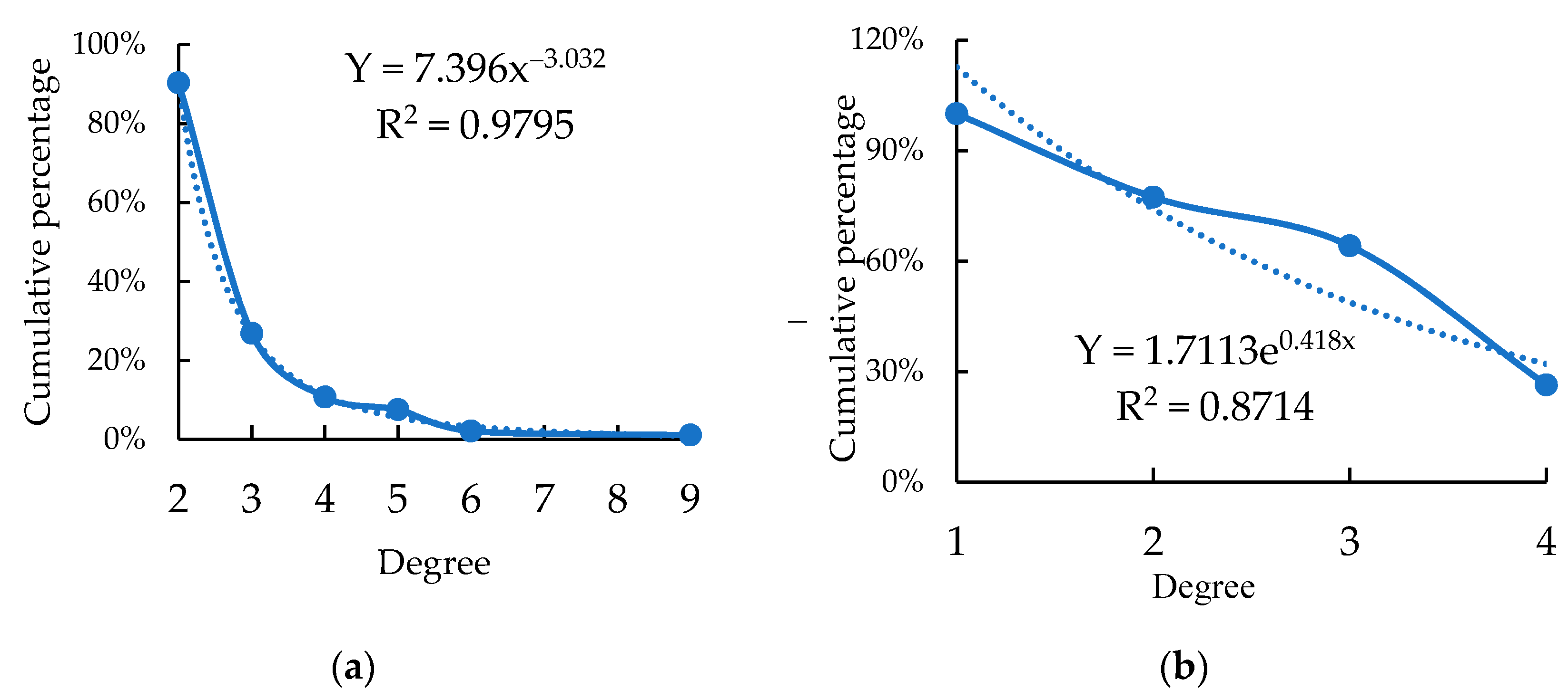
A scale-free network is usually determined by the cumulative degree distribution curve with a power-law characteristic. The cumulative degree distribution is calculated by:
where, k represents the degree, represents the distribution probability of nodes with degree value of k′, and represents the cumulative distribution probability of nodes with a degree not less than k. The cumulative degree distribution curve is drawn with as the vertical axis and k as the horizontal axis.
The cumulative degree distribution curves of the two typical networks are shown in Figure 2. The North China network has obvious power-law distribution characteristics, and the curve shows a rapid decline in the front section and a “long tail” phenomenon in the latter section. However, the European network deviates from the power-law distribution characteristics and the curve pattern tends to an exponential distribution. Through curve fitting, the power-law function fitted to the cumulative degree distribution of North China network is , with an R-square value exceeding 0.97 (the deviation point with a degree value of 1 accounting for 9.67% is deleted). The exponential function fitted to the cumulative degree distribution of European Network is , with an R-square value of 0.87. The range of its exponential power values is consistent with similar sparsely distributed networks, such as water supply networks [5] and urban road networks [26].
To sum up, the North China network is a scale-free network and the European network is a single-scale network. Scale-free networks have a few central-points with high degrees, which are robust to random failures, but very sensitive to the failures of central-points [2]. Therefore, the management of North China network should focus on the central-points. By finding the central-points (key stations), hierarchical management and control methods should be carried out. Safeguard measures could be taken to prevent the failure of central-points from causing a substantial decrease in the overall network performance. At the same time, optimization measures could be taken to reduce the importance of central-points and share their risks with the other nodes. To achieve this, the network structure can be optimized toward “decentralization” by improving path redundancy and other measures. The management of a single-scale network depends on the heterogeneity of the distribution. In fact, the European network is heterogeneous. For example, the first and second largest node distribution probabilities correspond to the second and first largest degree, respectively. When random failures occur, nodes with a high degree are more likely to fail due to their high distribution probability. Since degree can be regarded as the importance of node, the heterogeneity of the European network makes it very vulnerable to random failures. The European network management should focus on reducing its heterogeneity to ensure the system’s robustness.
3. Overall Structural Characteristics Evaluation
Usually, the constructed complex network model is represented by where G is the graph model, is the set of n nodes in the model, and is the set of m edges in the model. According to the physical properties of natural gas pipeline networks, this paper uses multiple indexes to analyze the overall structural characteristics of nodes, edges and their connectivity relationships. The calculation results for each index are listed in Table 3.
3.1. Analysis of Structural Redundancy
For a natural gas pipeline network, structural redundancy means that there is more than one path between nodes. The redundancy is very important for energy security. If there is only one path for a pair of nodes, the operator should pay more attention to this path. The shutdown of any edges and nodes along the path would cut off the natural gas supply to end users, which has occurred at times due to pipeline failures, political conflicts, hacker attacks, etc. In order to reduce the influence caused by pipeline failure, the redundancy of the system is usually increased by laying multiple parallel pipelines, building joint construction stations, adding interconnecting pipes between different pipelines, and constructing bridge valve rooms.
The edge density is applied here to evaluate the redundancy of the network. Given a certain number of nodes in a network, a higher edge density represents more paths between nodes and greater network redundancy. Edge density is calculated by:
This is the ratio of the actual number of edges to the theoretical maximum number of edges between nodes [15]. The value of edge density is between 0 and 1. An edge density of 1 means that any two nodes can be directly connected without going through other intermediate nodes, i.e., a fully-connected network. Since fully-connected network represents the most complex network form of network for a given number of nodes, the value of q can be used to measure network complexity quickly. Further, a more subtle method combining edge density and structure entropy is proposed [27]. Fractal theory is also a possible approach. The theory analyzes the network geometry characteristics of self-similar spatial distribution, and the self-similarity can be expressed with the fractal dimension, which quantifies the network complexity [7]. In this paper, the box-counting method based on the FracLab toolbox of Matlab language is applied to calculate the fractal dimensions of the two typical networks. By calculation, the fractal dimensions of the North China network and European network are 1.234 and 1.225, respectively, which are less than the published values for power grids [28] and water distribution networks [7]. The comparison results support the above judgment, that is, natural gas pipeline networks usually have a relatively simple topology.
As shown in Table 3, the edge density values of the two typical networks are far less than 1. The direct connections between nodes are very sparse, leaving much potential for interconnection optimization in the future. Moreover, the edge density of European Network is 2.5 times that of the North China network. The European network as a whole may be more redundant.
To further assess the redundancy of the networks, the loop density of edges was analyzed. The existence of loops makes the network more reliable, so the removal of an edge in the loop does not affect the connection between nodes in the entire loop system. The more loops a network has, the more options there are for gas flow between any two nodes and the greater the redundancy or reliability. As shown in Figure 1, the two typical natural gas pipeline networks have loops in various shapes, such as triangles, quadrilaterals, polygons and honeycombs. To quantitatively evaluate the loop density, the meshedness coefficient () is applied in this paper. Unlike the traditional ternary clustering coefficient which can only calculate the loop density of triangles, the meshedness coefficient includes all types of loops in the calculation and is more suitable for natural gas pipeline networks. The meshedness coefficient in the network is defined as the actual number of independent loops divided by the maximum possible number of independent loops with the same number of edges and nodes. Since the two typical networks have multiple gas sources, according to Euler’s theorem and its inference, the meshedness coefficient of the multi-source network is calculated by:
[16].
As shown in Table 3, the values of the two typical networks are both small and far less than the maximal value of 1, indicating again that the two typical networks are sparse. In addition, the of the European network is 1.8 times that of the North China network, showing that the European network has a higher degree of mesh structure and a greater probability of an edge in the loop. Therefore, the path redundancy of the European network may be greater.
3.2. Analysis of Structural Shape
Different structural shapes have different properties and characteristics. The edge per node ratio is represented by the equation [5]:
The overall structural shape of the network can be quickly judged by using or average node degree (its value is twice as large as ). For planar graphs, the value of is between 1 and 2. If the value is closer to 1, the structure of the network is more likely to have a characteristic tree shape or multi-star shape. If the value is closer to 2, the structure of the network is more likely to present the mesh shape. For natural gas pipeline networks, the mesh structure evenly distributes flow and line-pack. When an edge fails, it is not easy to interrupt the overall gas transmission. To a certain extent, a larger value represents higher hydraulic transmission efficiency and greater transmission robustness. As shown in Table 3, the values of the two typical networks are both closer to 1, showing their structures tend to have the tree shape. Generally, the total path length of a tree-shape network is relative short, which reflects the consideration of cost reduction during design since long path lengths increase the cost of land acquisition and pipeline laying. In addition, the structure of the tree-shape network can be easily optimized by future interconnections. However, when the “tree root” of the network fails, there is a greater impact on the entire network. Based on this, as shown by the previous redundancy analysis, the two typical networks both add some loops to the tree structure to reduce such effects. Because the overall loop density is smaller, the value of is greater than 1 but differs from the median value of its distribution range, which is 1.5. The actual value reflects the consideration of overall robustness in design, but the focus is still on cost control. By comparison, the of the European network is larger, showing transmission efficiency may be higher, and the structural robustness may be greater.
Center-point dominance quantifies the degree that a network structure converges toward a center, and can also be used to evaluate the network shape. It is calculated by:
where refers to the betweenness of node i, and is the maximum betweenness among all nodes [17]. The betweenness of a node is usually used to describe the centrality of a node. It is defined as the ratio of the number of paths passing through the node in all the shortest paths to the total number of shortest paths. Intuitively, the size of the betweenness reflects the importance of the node as a “bridge”. The value of is between 0 and 1. For starlike networks, . For regular networks, the betweenness centrality of all nodes is consistent, . Generally, when the overall structure of the network is closer to the star-like shape, the distance between nodes is shorter, the transportation is more direct, and the construction cost is lower. For a star-like network, however, the paths between all nodes in the network are disconnected and the entire system collapses if the central node fails (disconnecting it from its adjacent nodes). As shown in Table 3, the values of for the two typical networks are close but less than the median value of 0.5. These results are consistent with the tree structure with loop supplementation in the two typical networks discussed above. Again, the results reflect the two factors considered in the designs. That is, for natural gas pipeline networks, it is important to reduce costs, but the overall robustness should also be considered. Therefore, the pure star-like network is rarely used, although it has the lowest cost.
3.3. Analysis of Degree Characteristics
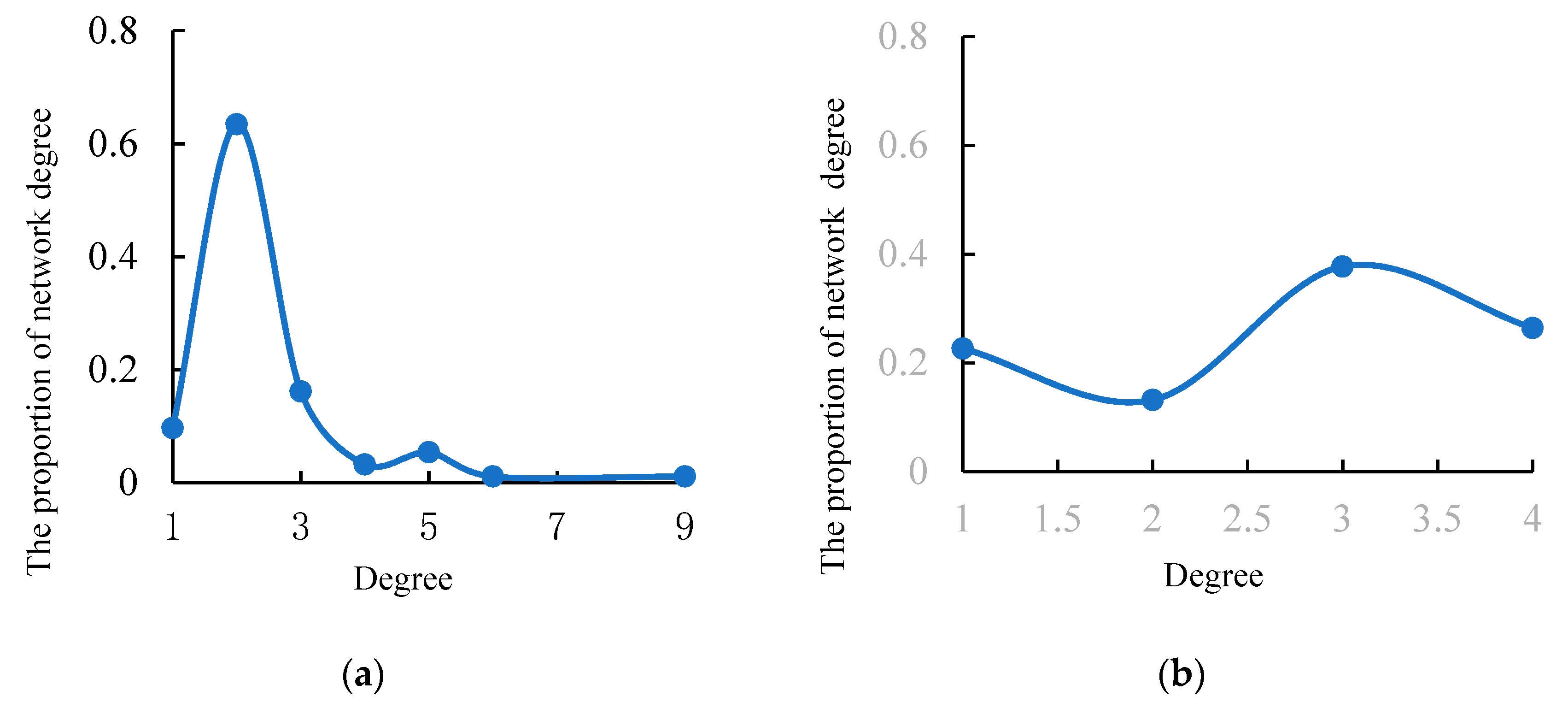
The average degree and distribution of degree reflect the overall structure characteristics of the network. As shown in Table 3, since the difference between the average degree value is small for the two typical networks, the degree distribution curves are proposed. As shown in Figure 3, for the North China network, the range of degree values is large and the distribution of degrees is uneven. The degree values of 6 and 9, which correspond to the second and first biggest value respectively, both have only one node. As the degree can be regarded as the importance of a node to the structure, from the perspective of structural robustness, it is disadvantageous for the natural gas pipeline network if the degree of some nodes is too large, and the optimal situation is achieved when each node has the same degree, which means each node is equally important. In optimal case, the failure of a node does not cause a significant decrease in the overall performance of the system. The operators should prevent those stations from targeted attacks or technical failures in order to guarantee the overall performance. In contrast, for the European network, the maximum degree value is 4, which is far less, and the degree distribution fluctuates in a relatively small range. In summary, from the point of view of the distribution of degree, the European network as a whole may have better structural robustness.
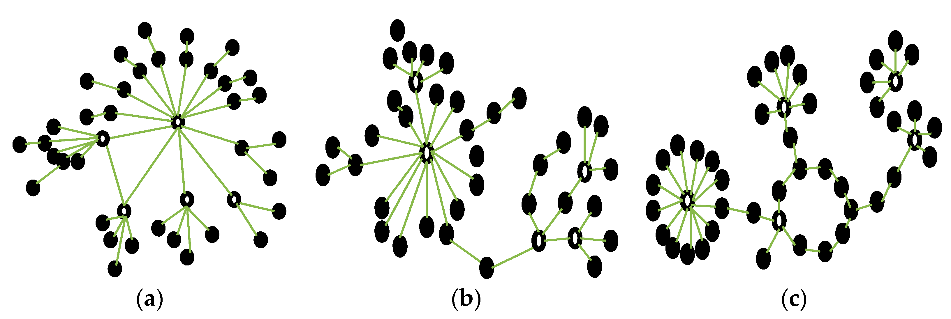
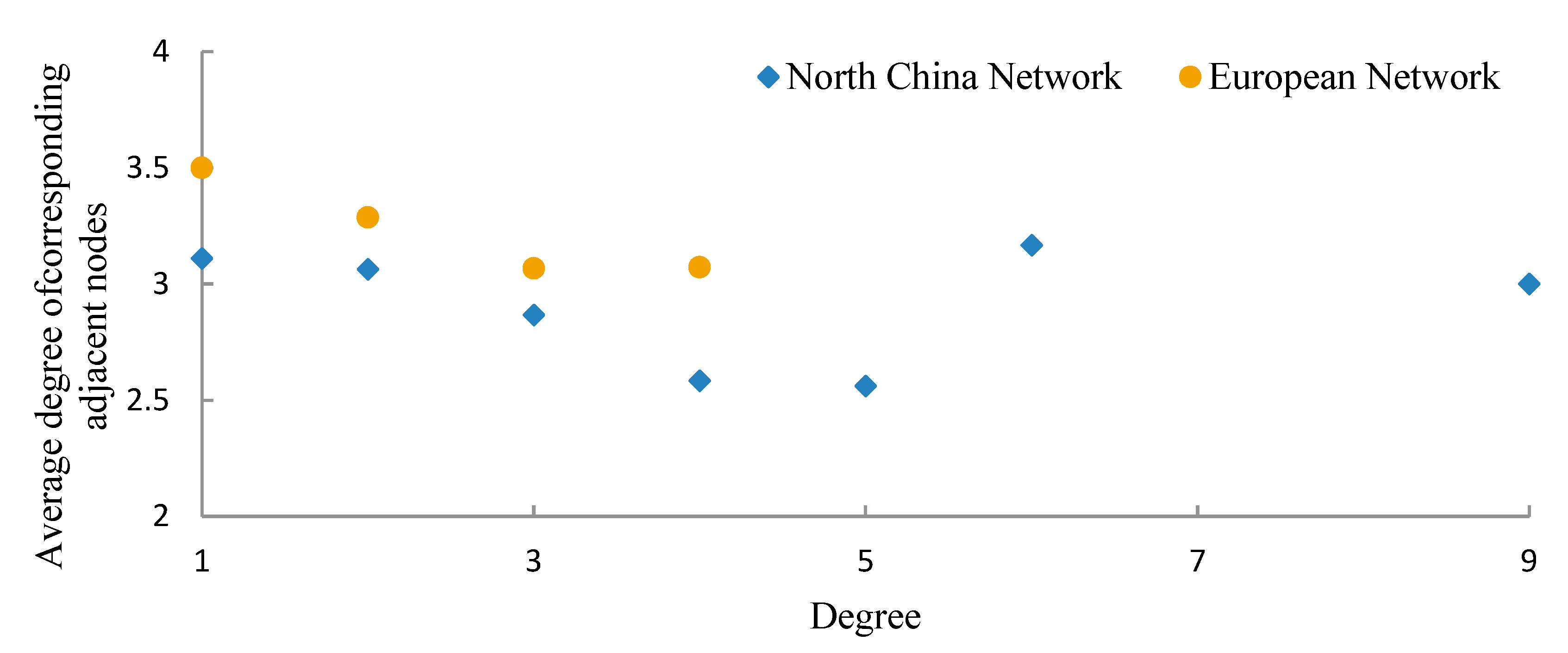
Concerning the relationship between the degree and connection of nodes, if the connection between all pairs of two nodes in a network is not related to the degree, then the network is considered degree-uncorrelated. Otherwise, the network is degree-correlated. As shown in Figure 4, for the degree correlated cases, if nodes with a large degree tend to connect nodes with a large degree, the network is said to have assortativity. In the opposite scenario, the network has disassortativity. To intuitively analyze the degree correlation of the two typical networks, the scatter plots of degree correlation were drawn. As shown in Figure 5, the horizontal axis represents the degree of a node, and the vertical axis represents the average degree of all adjacent nodes of this node. Seen from Figure 5, the curves of the two typical networks do not show a clear upward (assortativity) or downward (disassortativity) trend, indicating that the two typical networks are not highly degree correlated. To quantify degree correlation, this paper uses the assortative coefficient r, which is a degree-based Pearson correlation coefficient [18]. The value of r is between −1 and 1. Among the values, 1 indicating that a network has complete assortatvity, 0 indicating that a network is degree uncorrelated, and −1 indicating that a network has complete disassortativity. As shown in Table 3, the r value of the North China network is −0.05, which is near degree uncorrelated; the r value of the European network is −0.12, which represents a very slight disassortativity. The r values are similar to some electric power grids. For example, the r of a high-voltage grid in the west of the United States is −0.003 [29]. Obviously, there is no assortativity as found in social networks in which “people with a wide range of friends tend to have relationships with each other”. In addition, since a degree-correlated network has “cohesiveness”, as seen in Figure 4, the connection between node groups is weak, usually through only a single path. The failure of this single path leads to the failure of the corresponding node groups. Therefore, for natural gas pipeline networks, degree-correlated networks should be avoided.
4. Path-Related Structural Characteristics Evaluation
Analysis of path-related structural characteristics is very important for natural gas pipeline networks as it can, to some extent, reveal the transmission efficiency. Path distributions with short lengths contribute to reducing construction costs at the design stage and decreasing the transmission distance so as to lower energy consumption at the operation stage.
There are generally two measures of path length. One is the Euclidean distance in which each edge is weighted by the true length of the corresponding pipeline. The second is the geodesic distance in which each edge is not weighted, i.e., weight is 1.
In this paper, the network diameter, and the average shortest path length before and after weighting are calculated. The results are listed in Table 4.
The network diameter d is defined as the maximum value of the shortest path length between two nodes in the network, expressed by the geodesic distance [19]. It measures the separation degree of two furthest nodes in a network. As shown in Table 4, the diameters of the North China network and the European Network are close, with the values of 19 and 17, respectively.
According to the previous definition, the average path length is the average of the shortest path lengths between all pairs of nodes. L1 and L2 represent the average path length before and after weighting, respectively. As shown in Table 4, although the two typical networks have many nodes, L1 is only a single digit, which is consistent with the characteristics of a small-world network as determined in the previous analysis. Since any two nodes can be connected to each other through a few edges, the transmission efficiency of natural gas pipeline network can be ensured to some extent. Analyzing L2, the weighted average path lengths of the North China network and the European network are 441.99 km and 370.43 km, respectively. The designers of both networks tend to maintain the average path length at around 400 km. By comparison, the L1 and L2 of the European network are both smaller than those of the North China network, indicating that the shortest paths in the European network have fewer edges and shorter pipeline lengths. According to the Darcy equation, the route energy loss and transmission path length are positively correlated. Therefore, the shorter lengths result in a smaller route energy loss, leading to a higher transmission efficiency.
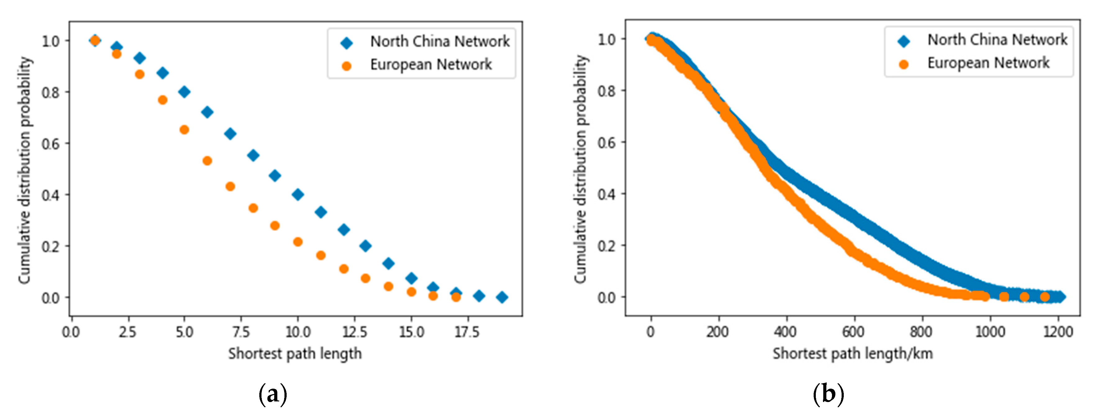
L1 and L2 both are the average value. When using the average value for analysis, researchers should be careful. If there is a distortion point in the numerical distribution, the average value will be distorted, which will affect the overall assessment. For example, if a sample point with a value of 10,000 is added to a set of 100 sample points with an average value of 1, the average value will be enlarged to 100. Clearly, in this case, it is meaningless to use the average value to analyze the overall characteristics. To overcome this drawback, it is necessary to further analyze the distribution of shortest path length between nodes. Figure 6 shows scatter plots of the cumulative distribution of the shortest path length between nodes before and after weighting. The horizontal axis represents the shortest path length and the vertical axis represents the cumulative distribution probability. From the perspective of curve shape, the weighted curves (Figure 6b) can be roughly divided into three sections with different slopes. In the first section, the curves decrease rapidly; in the middle section the curves show a slower downward trend, and in the last section the curves are close to horizontal line. The first sections of the two typical networks are close to overlapping, and the inflection points between first section and middle section both appear at a shortest path length of about 350 km. The corresponding cumulative distribution probabilities of the inflection points are both about 0.5. This indicates that nearly half of the shortest path length between nodes is less than 350 km so that the transmission efficiency is guaranteed to a certain extent. The middle sections of the two typical networks are quite different as the European network is significantly lower than the North China network. In this section, under the same cumulative distribution probability, the shortest path length between nodes in the European network is smaller. The inflection points between the middle and last section of the North China network and the European network are around 1000 km and 800 km, respectively, and the corresponding cumulative distribution probabilities are both close to 0, indicating that designers try to avoid long-distance transmission. In the last section, the curve shapes of the two typical networks are both close to the horizontal line and the European network is more sparsely distributed. In terms of the maximum shortest path length values, the North China network and the European network are similar with values of 1205.39 km and 1162.60 km, respectively. It is worth noting that the longest length for a single pipeline in the North China network is 1302 km, which is close to the maximum shortest path length. It shows that although the network loops increase the redundancy, they do not effectively reduce the maximum value of the transmission distance. As transmission distance impacts efficiency to some extent, designers not only need to consider adding redundancy, but also pay attention to decreasing the transmission distance in later interconnection construction. To sum up, the weighted shortest-path length of the European network is shorter in the middle section and the distribution is sparser in the last section (corresponding to large shortest-path-length distribution). This pattern results in the European network having a smaller L2. For the unweighted curves, the shapes of the two typical networks are similar to the weighted ones, and the overall curve position of the European network is relatively lower. By analyzing the distribution of L1 and L2, we reconfirm the above conclusion that the European network has a higher transmission efficiency.
5. Structural Robustness Characteristics Evaluation
Structural robustness refers to the degree to which a network can withstand components (nodes or edges) removal without affecting its connection. As shown in Figure 1, due to the complex structure, different components in a network have different importance. Usually, there are some key components, such as the degree-based hubs, in the natural gas pipeline network. Once they fail, it is extremely destructive to the connectivity, transmission efficiency, even leading to a lack of supply to customers.
In recent years, there have been many “gas shortage” incidents in the world due to the lack of robustness, i.e., pipe failures leading to disconnection of the network topology. In 2009, Ukraine shut down three Russian gas pipelines to the EU via Ukraine for two weeks, reducing Russia’s gas supply to the EU by about 1/7 [30]. In 2011, due to the political conflict in Libya, the country’s natural gas pipeline supplying Italy with an annual designed capacity of 8 billion m3 was interrupted for 8 months [31]. In 2022, the Russia-Ukraine conflict has brought a sharp rise in EU natural gas price.
To the author’s knowledge, in the design review stage of pipeline construction, operators still regard reducing construction costs as the highest priority, usually ignoring or underestimating the importance of robustness. However, emergencies and natural or man-made catastrophes may occur at any time so operators cannot completely avoid failures even if they have made efforts take precautions. If historical events such as supply shortages occur again due to a lack of robustness, the whole society will pay an inestimable economic cost. Therefore, it is recommended that robustness be considered in the design and subsequent network optimization to build more robust natural gas pipeline networks, i.e., networks with more redundant paths between nodes, fewer central nodes, and layouts with a higher mesh degree.
When evaluating the robustness of the two typical networks, several traditional methods have some problems. The analysis is as follows.
5.1. Edge (Node) Connectivity Evaluation Method
The edge (node) connectivity of the network is the most direct and important index for quantitatively evaluating structural robustness. It is defined as the minimum number of failed edges (nodes) that disconnect the connected network [32]. Smaller edge (node) connectivity usually represents a lower level of structural robustness. When an edge (node) fails, a network with smaller edge (node) connectivity more readily disintegrates. Based on complex network theory, the calculation of edge (node) connectivity can be transformed into the problem of identifying cut sets. A cut set is a collection of edges (nodes), in which the failure of edges (nodes) will cause the originally connected complex network to split into inter-disconnected sub-networks. If the cut set consists of a series of single edges, the corresponding edges are called bridge edges. If a cut set consists of a series of individual nodes, the corresponding nodes are called cut nodes. Intuitively, a cut node or bridge edge refers to a node or edge that does not belong to any loop. For a natural gas pipeline network, when the station fails, the gas flow crosses the failed station through a bypass pipe, which will not have a great impact on the overall transmission. Even if the compressor station fails, it only affects about 20% of the pipeline transmission capacity [13]. In contrast, the failure of one pipe segment causes the complete shutdown of gas transmission in this pipe section. Based on this, the edge cut set should be first studied. According to our analysis, the two typical networks both have bridge edges and their location has been identified. As shown in Figure 7, the bridge edges (red-colored edges) of the two typical networks are located at the end or beginning of the network, corresponding to end users or gas sources. If the bridge edges connect the main gas sources, important factories and big cities, there is a substantial risk to gas supply for the whole system. When the bridge edge fails, the corresponding users or gas sources are disconnected from the entire network, affecting the import or sale of natural gas. However, there is no bridge edge on the belly of the network. This shows that designers take the interconnection construction into account for the main pipelines, ensuring the main pipelines connection will not be affected after failure of one pipe segment. From the perspective of improving the structure robustness, it is necessary to build redundant pipelines connecting sources or users. Therefore, bridge edges should be eliminated first, and all nodes should be connected by at least two pipelines. For the multinational pipelines, it is recommended to deploy redundant pipelines in different regions to avoid geo-political risk. Our analysis reveals that the two typical networks also have cut nodes. In summary, the existence of bridge edges and cut nodes leads to some unique paths between corresponding nodes. They are the key control concern for the pipeline network, and their reliability should be improved to avoid failures. More importantly, the existence of bridge edges and cut nodes makes the edge (node) connectivity of the two typical networks equal to 1, which cannot be compared and analyzed. Therefore, the quantitative evaluation of the structural robustness for the natural gas pipeline network requires other methods.
5.2. Direct Method
The direct method is to delete network components directly, and then calculate the corresponding index after deletion, so as to evaluate whether the components are important or not [33]. The results are intuitive, accurate, and easy to analyze and explain. In order to quantify the importance, different “centrality indexes” have been proposed based on different physical meanings. The importance of the deleted components is usually quantified by comparing the centrality index difference before and after deletion [34]. Considering transmission efficiency, this paper adopts L2 as the centrality index and takes one-edge failure as the analysis object. The direct method includes the following steps:
- (1)
- Initialize an empty list (called R).
- (2)
- Initialize the network topology model with natural gas pipelines data
- (3)
- Calculate the L2 of the initial model.
- (4)
- Identify the bridge edges of the initial model.
- (5)
- for edge in edges (loop every edge of the initial model).
- (6)
- Determine if an edge is not in bridge edges (deletion of bridge edge disconnects the model, leading to infinite L2).
- (7)
- Delete this edge from the initial model.
- (8)
- Calculate the L2 of the edge deleted model.
- (9)
- Calculate the ratio of the initial model L2 to edge deleted model L2.
- (10)
- Append the ratio result to the list R.
- (11)
- End the for loop.
- (12)
- Sort the list R in an ascending order.
- (13)
- The results are obtained according to the list R and other auxiliary data.
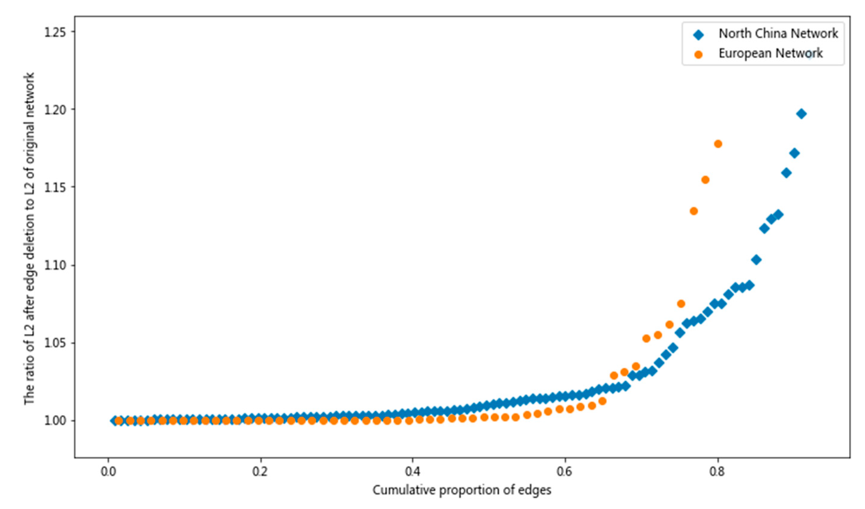
Figure 8 shows the results of the two typical networks by this direct method. The horizontal axis represents the cumulative proportion of edges and the vertical axis represents the ratio of L2. From the shape of the curves, the two typical networks can be roughly divided into two sections with different slopes. The left section of the curve is almost horizontal, and the ratio of L2 is close to 1. This indicates that when removal of an edge in this section occurs, there are alternative paths between nodes and the length of the alternative shortest path is close to the original one. Therefore, the removal of this edge has almost no impact on the overall connection or even transmission efficiency. In comparison, the European network curve in the left section has a smaller slope, which may indicate a greater structural robustness than for the North China network. However, in the right section, the inflection point of the European network curve appears earlier and the curve has a steeper slope. On the far right, due to the existence of bridge edges, the cumulative proportion of edges for both networks cannot reach 100.00%. According to our calculations, the bridge edges of the European network account for 21.12%, whereas the value for the North China network is 10.25%. Therefore, the right section of the curves suggest that the structural robustness of the North China network is greater, which contradicts the analysis result for the left section. In summary, for the two typical pipe networks, analyses of the two sections lead to different results, which requires careful consideration. In short, the analysis by the direct method may cause some confusion.
5.3. Percolation Theory Method
The percolation theory method is widely used to analyze transportation systems [35,36,37]. The process of gradually removing nodes or edges one-by-one from a network is called site or bond percolation. In reality, the components removal represents their failure. The simplest and classic measure to remove nodes or edges is complete random deletion. During the percolation process, when the largest connected subgroup disintegrates into several subgroups, the proportion of accumulated failed nodes or edges-threshold— is calculated [14].
This threshold can be used to evaluate the robustness of the topology. If the proportion of accumulative failed nodes or edges is below the threshold, although some parts of network are isolated, the existence of largest connected subgroup ensures that at least a large part of the network is connected so as to maintain its main performance. If the proportion of accumulative failed nodes or edges is not less than the threshold, the network has lots of small mutually disconnected subgroups. In this state, the original network topology has been divided into pieces and each node at most connects a few other nodes. The main performance will collapse. Therefore, a large threshold indicates a network could maintain the overall performance even after removing many nodes or edges, i.e., a network has strong robustness. In contrast, weakly connected networks usually exhibit low thresholds. The removed node or edge at the threshold moment can be regarded as a candidate of bottleneck or weaky-connected section, since its removal causes the collapse of the network.
Other removal measures are also used such as deletion by degree. It should be noted that different removal measures or even each run of random removal will result in different thresholds.
In this paper, the theoretical formula from the literature is used to calculate the threshold of random node failure, which is:
[20].
As shown in Table 5, the European network has a higher value. In the case of random failure, theoretically, 53% of nodes suffering simultaneous failure will cause the collapse of the network. From this index, it can be concluded that structural robustness of the European network may be greater. In fact, natural gas pipeline networks and transportation networks are different in nature. For transportation networks, a highway can be considered failed when it reaches a given congestion degree, and it is common for multiple roads to be congested at the same time. However, for natural gas pipeline networks, it is only theoretically possible for several or even dozens of edges (nodes) to fail at the same time. Therefore, the percolation theory method, which is widely used in the transportation system, is not applicable to the natural gas pipeline network.
5.4. Alternative Indexes Method-Algebraic Connectivity and Spectral Gap
Since the three conventional methods are not applicable to the two typical networks, this paper adopts alternative connectivity indexes, namely algebraic connectivity and spectral gap. They are not related to the scale of pipeline and the drawing style of network topology. They can quantitatively evaluate the network connectivity and reflect the network robustness to a certain extent.
The algebraic connectivity is defined as the second smallest eigenvalue of the Laplacian matrix of a network since the smallest value is 0 [20]. The Laplacian matrix of a network can be calculated by Lap = D − A, where , represents the diagonal matrix, represents the degree of node i, and A represents the adjacency matrix of a network.
Scholars apply this index to the network robustness analysis for the failure of edge or node. It is also used to measure the network connectivity for networks with the same number of nodes and edges but different connections [38]. Larger represents a stronger structural connectivity and greater robustness to edge or node failure [15,16].
The spectral gap is defined as the difference between the first eigenvalue and the second eigenvalue of the network adjacency matrix. The value of the spectral gap can evaluate whether a network has good expansion [39]. In terms of network topology, good expansion means no matter whether the distribution is sparse or not, any node has been connected to other nodes in an optimal way. Larger value of indicate better network expansion, more uniform distribution of node degree, more optimized nodes connection, smaller node or edge failure impacts, and greater network structural robustness. Conversely, a smaller is usually accompanied by lower connectivity or the existence of many bridge edges and cut nodes whose failure will disintegrate the network [40].
As shown in Table 5, and values for the European Network are both larger than those of the North China network, indicating the robustness of the European network may be better. It is worth noting that the magnitude of for the two typical networks is small, indicating a lack of good expansion and reflecting the lack of overall robust optimization in the design process. For example, the four Shaanxi–Beijing natural gas pipelines of the North China network came into operation in 1997, 2005, 2010 and 2017, respectively. Each pipeline was designed and constructed separately according to the changes in gas demand in different periods. Therefore, in addition to building new pipelines to meet new demands, robustness optimization of existing pipelines also cannot be ignored.
6. Discussion and Conclusions
In this paper, complex network theory was used to analyze the topology of natural gas pipeline networks. The complex network topology model was established based on typical networks in North China and Europe. For the first time, the topology model of the natural gas pipeline network in North China has been established in academic research. This paper screens different indexes using complex network theory according to the physical nature of a natural gas pipeline network. A comprehensive and comparative analysis of typical network topological structures is performed from the perspectives of network type, overall topological structure characteristics, path-related topological structure characteristics, and topological structure robustness. The topology analysis framework for natural gas pipeline networks developed in this paper is summarized in Figure 9.
In fact, the purpose of natural gas pipeline networks is to transport natural gas. A comprehensive analysis must consider the network topology, hydraulic characteristics, and uneven distribution of supply and demand together. Different compressor startup strategies and different relationships between supply and demand will lead to different pressures on the pipeline network, affecting the transmission of natural gas. However, the topology can reflect the natural gas network transmission characteristics in an approximate way. For example, shorter path lengths and greater redundancy may represent more uniform pressure distribution, smaller pressure loss, and higher transmission efficiency. Analysis of the correlations between the topological attribute metrics and hydraulic metrics should be performed in future studies. In addition, the topology analysis of a natural gas pipeline network based on complex network theory is rapid and efficient. Therefore, a topology analysis should be conducted as the first step in the study of a network. It not only facilitates an intuitive understanding of the network, but also provides a solid foundation and guidance for subsequent optimization and hydraulic calculation. It is also worth noting that although this paper uses many indexes to analyze the two typical networks, the comparative analysis method for the two typical networks can be used to analyze the effects of optimizing measures on a given network. Although the framework is proposed for topology analysis of natural gas pipeline networks, it is applicable to similar networks such as hydrogen, natural gas synthesis, and carbon dioxide transmission networks, since they are all gas transmission systems that transport gas from sources to users by pipeline and the same basic flow equations and similar topological considerations are applicable.
The comprehensive and comparative analysis results of the two typical networks topology are concluded as follows, and the main index values are summarized in Table 6.
- (1)
- Considering network type, the two typical networks are both small-world networks. According to the distribution characteristics of cumulative degree, the North China network is a scale-free network with strong heterogeneity, while the European network is a single-scale network.
- (2)
- For overall topological structure characteristics, although the distribution of two typical networks is somewhat redundant and the shape presents a tree structure supplemented by loops, the networks as a whole are sparsely distributed. Additionally, the two typical networks both show very slight disassortativity, and are close to degree uncorrelated.
- (3)
- Considering path-related topological structure characteristics, the shortest path length distribution curves for the two typical networks before and after the weighting were drawn. After weighting, the curves show a three-section pattern, the curves in the first section decline rapidly, the downward trend in the middle section becomes slow, and the curves in the last section are close to the horizontal line. In terms of average value, designers appear to maintain the average path length at around 400 km. In terms of the maximum value, although the loop design in the North China network increases the redundancy, it does not effectively reduce the maximum value of the pipeline transmission distance. It is suggested that apart from redundancy, transmission distance optimization should be considered in the subsequent reconstruction. Without weighting, the curves show a two-stage feature with a rapid decline section followed by a near plateau section.
- (4)
- Considering topological structure robustness, the topological bridge edges and cut nodes of the two networks are identified. It is suggested that bridge edges should be eliminated first in later reconstructions to improve the network robustness. The traditional connectivity index, direct method and percolation theory method are not applicable to the robustness evaluation of the two typical networks due to the existence of bridge edges and cut nodes, the special curve shape of the direct method based on L2, and the extremely low probability of simultaneous failure of multiple edges, respectively. However, the robustness can be quickly and efficiently evaluated using alternative connectivity indexes, namely algebraic connectivity and spectral gap.
- (5)
- Through quantitative comparison and analysis of the topological structure evaluation indexes, it is clear that the European network has a higher loop density, more uniform node degree distribution, smaller average shortest path lengths both before and after weighting, and larger alternative connectivity indexes. These results show that the redundancy, transmission efficiency and robustness of the European Network are greater than those of the North China network.
Author Contributions
Conceptualization, H.Y.; Methodology, H.Y.; Supervision, Z.L.; Visualization, G.L.; Writing—original draft, H.Y.; Writing—review & editing, Y.L. All authors have read and agreed to the published version of the manuscript.
Funding
This research was funded by National Natural Science Foundation of China grant number 51904316.
Institutional Review Board Statement
Not applicable.
Informed Consent Statement
Not applicable.
Data Availability Statement
Not applicable.
Conflicts of Interest
The authors declare no conflict of interest.
Nomenclature
| LNG | Liquefied Natural Gas |
| Node | |
| Node | |
| The shortest path length between node and node | |
| The degree of node | |
| Clustering coefficient of node i | |
| Average clustering Coefficient | |
| The degree of node | |
| The actual number of edges between node and its adjacent nodes | |
| Degree | |
| The distribution probability of nodes with degree value of k’ | |
| The distribution probability of nodes with degree no less than k | |
| The set of n node in network | |
| n | The number of nodes in network |
| The set of m edges in network | |
| m | The number of edges in network |
| q | Edge density |
| e | Edge per node ratio |
| kmax | Maximum degree |
| Central-point dominance | |
| M | Meshedness coefficient |
| r | Assortativity coefficient |
| The maximum betweenness of all nodes | |
| Threshold for random removal of nodes | |
| λ2 | Algebraic connectivity |
| Spectral gap | |
| Lap | The Laplacian matrix of the network |
| A | The adjacency matrix of network |
References
- Xu, J. Research on Network Vulnerability of Urban Rail Transit System. Ph.D. Thesis, Beijing Jiaotong University, Beijing, China, 2020. [Google Scholar]
- Albert, R.; Jeong, H.; Barabási, A.-L. Error and attack tolerance of complex networks. Nature 2000, 406, 378–382. [Google Scholar] [CrossRef] [PubMed] [Green Version]
- Li, W.; Xu, S.; Wang, Y. Analysis of New York Rail Transit Network Characteristics Basedon Complex Network. Comput. Mod. 2021, 2, 94. [Google Scholar]
- Zou, Z.; Xiao, Y.; Gao, J. Robustness analysis and optimization of urban public transport network based on complex network theory. Kybernetes 2021, 42, 1–6. [Google Scholar]
- Yazdani, A.; Jeffrey, P. Complex network analysis of water distribution systems. Comput. Eng. Appl. 2011, 21, 016111. [Google Scholar] [CrossRef] [PubMed] [Green Version]
- Yazdani, A.; Jeffrey, P. Robustness and Vulnerability Analysis of Water Distribution Networks Using Graph Theoretic and Complex Network Principles. In Proceedings of the Conference on Water Distribution Systems Analysis, Tucson, AZ, USA, 12–15 September 2010. [Google Scholar]
- Santonastaso, G.F.; Greco, R.; Giudicianni, C. Complex network and fractal theory for the assessment of water distribution network resilience to pipe failures. Water Supply 2018, 18, 767–777. [Google Scholar]
- Nardo, A.D.; Natale, M.D.; Giudicianni, C.; Musmarra, D.; Santonastaso, G.F.; Simone, A. Water Distribution System Clustering and Partitioning Based on Social Network Algorithms. Procedia Eng. 2015, 119, 196–205. [Google Scholar] [CrossRef] [Green Version]
- Xu, T.; Chen, J.; He, Y.; He, D.-R. Complex network commonness of China’s power network. Sci. Technol. Rev. 2004, 22, 11–14. [Google Scholar]
- Bai, W.J.; Wang, B.H.; Zhou, T. Brief Review of Blackouts on Electric Power Grids in Viewpoint of Complex Networks. Complex Syst. Complex. Sci. 2005, 3, 29–37. [Google Scholar]
- Wang, W.; Zhang, Y.; Li, Y.; Liu, C.; Han, S. Vulnerability analysis of a natural gas pipeline network based on network flow. Int. J. Press. Vessel. Pip. 2020, 188, 104236. [Google Scholar] [CrossRef]
- Carvalho, R.; Buzna, L.; Bono, F. Robustness of trans-European gas networks. Phys. Rev. E 2009, 80, 016106. [Google Scholar] [CrossRef]
- Praks, P.; Kopustinskas, V.; Masera, M. Probabilistic modelling of security of supply in gas networks and evaluation of new infrastructure. Reliab. Eng. Syst. Saf. 2015, 144, 254–264. [Google Scholar] [CrossRef]
- Newman, M.E.J. Networks: An Introduction; Oxford University Press: Oxford, UK, 2013; pp. 376–378. 720p. [Google Scholar]
- Jamakovic, A.; Uhlig, S. On the relationship between the algebraic connectivity and graph’s robustness to node and link failures. In Proceedings of the Conference on Next Generation Internet Networks, Trondheim, Norway, 21–23 May 2007. [Google Scholar]
- Buhl, J.; Gautrais, J.; Reeves, N.; Solé, R.V.; Valverde, S.; Kuntz, P.; Theraulaz, G. Topological patterns in street networks of self-organized urban settlements. Eur. Phys. J. B-Condens. Matter Complex Syst. 2006, 49, 513–522. [Google Scholar] [CrossRef]
- Freeman, L.C. A Set of Measures of Centrality Based on Betweenness. Sociometry 1977, 40, 35. [Google Scholar] [CrossRef]
- Newman, M.E. Assortative Mixing in Networks. Phys. Rev. Lett. 2002, 89, 208701. [Google Scholar] [CrossRef] [PubMed] [Green Version]
- Costa, L.d.F.; Rodrigues, F.A.; Travieso, G.; Villas Boas, P.R. Characterization of complex networks: A survey of measurements. Adv. Phys. 2007, 56, 167–242. [Google Scholar] [CrossRef] [Green Version]
- Cohen, R.; Erez, K.; Ben-Avraham, D.; Havlin, S. Resilience of the Internet to Random Breakdowns. Phys. Rev. Lett. 2000, 85, 4626–4628. [Google Scholar] [CrossRef] [Green Version]
- Estrada, E. Network robustness to targeted attacks. The interplay of expansibility and degree distribution. Eur. Phys. J. B-Condens. Matter Complex Syst. 2006, 52, 563–574. [Google Scholar] [CrossRef]
- Erdős, P.; Rényi, A. On Random Graphs I. Publ. Math. 1959, 4, 3286–3291. [Google Scholar]
- Watts, D.J.; Strogatz, S.H. Collective dynamics of ‘small-world’networks. Nature 1998, 393, 440–442. [Google Scholar] [CrossRef]
- Barabási, A.-L.; Albert, R. Emergence of scaling in random networks. Science 1999, 286, 509–512. [Google Scholar] [CrossRef] [Green Version]
- Li, Z.; Yang, Z.; Liu, R. A review of combining complex networks and machine learning. Comput. Appl. Softw. 2019, 36, 10–28+62. [Google Scholar]
- Barthélemy, M.; Flammini, A. Modeling Urban Street Patterns. Phys. Rev. Lett. 2008, 100, 138702. [Google Scholar] [CrossRef] [PubMed] [Green Version]
- Lei, M.; Wei, D. An Improved Method to Measur the Complexity of Complex Network. J. Hubei Minzu Univ. 2019, 37, 5. [Google Scholar]
- Li, H.; Lyu, F.; Fan, H. Quantitative Structure Method for 500 kV/220 kV Power Grid Based on Fractal Dimension. Autom. Electr. Syst. 2015, 39, 87–92. [Google Scholar]
- Newman, M.E. Mixing patterns in networks. Phys. Rev. E 2003, 67, 26126. [Google Scholar] [CrossRef] [PubMed] [Green Version]
- Lochner, S. Modeling the European natural gas market during the 2009 Russian–Ukrainian gas conflict: Ex-post simulation and analysis. J. Nat. Gas Sci. Eng. 2011, 3, 341–348. [Google Scholar] [CrossRef]
- Lochner, S.; Dieckhöner, C. Civil unrest in North Africa—Risks for natural gas supply. Energy Policy 2012, 45, 167–175. [Google Scholar] [CrossRef] [Green Version]
- Kessler, A.; Ormsbee, L.; Shamir, U. A methodology for least-cost design of invulnerable water distribution networks. Civ. Eng. Syst. 1990, 7, 20–28. [Google Scholar] [CrossRef]
- Cadini, F.; Agliardi, G.L.; Zio, E. A modeling and simulation framework for the reliability/availability assessment of a power transmission grid subject to cascading failures under extreme weather conditions. Appl. Energy 2017, 185, 267–279. [Google Scholar] [CrossRef] [Green Version]
- Latora, V.; Marchiori, M. Vulnerability and protection of infrastructure networks. Phys. Rev. E 2005, 71, 015103. [Google Scholar] [CrossRef] [Green Version]
- Chen, Z.; Ma, S.; He, M. Identification of Dynamic Service Bottleneck in UrbanRailway Network Based on Traffic Percolation Theory. China Transp. Rev. 2021, 43, 78–84. [Google Scholar]
- Wu, R.; Zhou, Y.; Chen, Z. Identifying urban traffic bottlenecks with percolation theory. Urban Transp. China 2019, 17, 96–101. [Google Scholar]
- Hamedmoghadam, H.; Jalili, M.; Vu, H.L.; Stone, L. Percolation of heterogeneous flows uncovers the bottlenecks of infrastructure networks. Nat. Commun. 2021, 12, 1254. [Google Scholar] [CrossRef] [PubMed]
- Meng, F.; Fu, G.; Farmani, R.; Sweetapple, C.; Butler, D. Topological attributes of network resilience: A study in water distribution systems. Water Res. 2018, 143, 376–386. [Google Scholar] [CrossRef]
- Ghosh, A.; Boyd, S. Growing Well-connected Graphs. In Proceedings of the 45th IEEE Conference on Decision and Control, San Diego, CA, USA, 13–15 December 2006; pp. 6605–6611. [Google Scholar]
- Donetti, L.; Neri, F.; Muoz, M.A. Optimal network topologies: Expanders, Cages, Ramanujangraphs, Entangled networks and all that. J. Stat. Mech. Theory Exp. 2012, 8, P08007. [Google Scholar] [CrossRef] [Green Version]
Figure 1.
Undirected topology diagrams of the two typical networks: (a) North China network; (b) European network.
Figure 1.
Undirected topology diagrams of the two typical networks: (a) North China network; (b) European network.

Figure 2.
Cumulative degree distribution curves of the two typical networks: (a) North China network; (b) European network.
Figure 2.
Cumulative degree distribution curves of the two typical networks: (a) North China network; (b) European network.

Figure 3.
Degree distribution curves of the two typical networks. (a) North China network; (b) European network.
Figure 3.
Degree distribution curves of the two typical networks. (a) North China network; (b) European network.

Figure 4.
Three kinds of degree correlation networks: (a) Assortative network; (b) Degree-uncorrelated network; (c) Disassortative network.
Figure 4.
Three kinds of degree correlation networks: (a) Assortative network; (b) Degree-uncorrelated network; (c) Disassortative network.

Figure 5.
Scatter plots of degree correlation for the two typical networks.

Figure 6.
Scatterplots of the cumulative distribution of shortest path length between nodes for the two typical networks: (a) Before weighting; (b) After weighting.
Figure 6.
Scatterplots of the cumulative distribution of shortest path length between nodes for the two typical networks: (a) Before weighting; (b) After weighting.

Figure 7.
Bridge edges diagrams of the two typical networks: (a) North China network; (b) European network.
Figure 7.
Bridge edges diagrams of the two typical networks: (a) North China network; (b) European network.

Figure 8.
Scatterplots of the ratio of L2 before and after one-edge deletion for the two typical networks.
Figure 8.
Scatterplots of the ratio of L2 before and after one-edge deletion for the two typical networks.

Figure 9.
The framework of topology analysis for natural gas pipeline networks.


Table 1.
Indexes used to analyze networks.
| Index | Definition | Equation | Analysis | Reference |
|---|---|---|---|---|
| Average path length | Average of the shortest path length between any two nodes (weighted or not) | Network type and path-related characteristics | Li et al. [3] | |
| Clustering coefficient | The actual number of edges between the adjacent nodes of node i divided by the theoretical maximum number of edges between those adjacent nodes | Network type | Newman [14] | |
| Edge density | The ratio of the actual number of edges to the theoretical maximum number of edges between nodes | Redundancy | Jamakovic and Uhlig [15] | |
| Meshedness coefficient | The actual number of independent loops divided by the maximum possible number of independent loops with the same number of edges and nodes | Redundancy | Buhl et al. [16] | |
| Edge per node ratio | The ratio of number of edges to number of nodes | Shape | Yazdani and Jeffrey [5] | |
| Center-point dominance | Average difference between most central node betweenness and all nodes betweenness | Shape | Freeman [17] | |
| Assortative coefficient | Degree-based Pearson correlation coefficient | Degree characteristics | Newman [18] | |
| Network diameter | Maximum geodesic shortest path length between any two nodes | Path-related characteristics | Costa et al. [19] | |
| Algebraic connectivity | Second smallest eigenvalue of the Laplacian matrix of the network | Robustness | Cohen et al. [20] | |
| Spectral gap | The difference between the first and the second eigenvalue of network adjacency matrix | Robustness | ESTRADA [21] |
Table 2.
Calculation results of small-world parameters of the two typical networks.
| L | C | |||||
|---|---|---|---|---|---|---|
| Related Random Network | Real Network | Related Regular Network | Related Random Network | Real Network | Related Regular Network | |
| North China network | 4.19 | 8.45 | 20.52 | 0.02 | 0.06 | 0.21 |
| European network | 2.97 | 6.48 | 18.29 | 0.06 | 0.17 | 0.30 |
Table 3.
Overall structural characteristic indexes of two typical networks.
| q | e | <k> | kmax | r | |||
|---|---|---|---|---|---|---|---|
| North China network | 0.02 | 1.19 | 2.39 | 9.00 | 0.38 | 0.10 | −0.05 |
| European network | 0.05 | 1.34 | 2.68 | 4.00 | 0.41 | 0.18 | −0.12 |
| Difference * | 2.50 | 1.13 | 1.12 | 0.44 | 1.07 | 1.80 | 2.40 |
* The corresponding index ratio of European network to North China network, rounded to two decimal places.
Table 4.
Path-related structural characteristics evaluation indexes of the two typical networks.
| d | L1 | L2/(km) | |
|---|---|---|---|
| North China network | 19.00 | 8.45 | 442.00 |
| European network | 17.00 | 6.48 | 370.43 |
| Difference * | 0.89 | 0.77 | 0.84 |
* The corresponding index ratio of the European network to the North China network, rounded to two decimal places.
Table 5.
Robustness characteristics evaluation indexes of the two typical networks.
| North China network | 0.49 | 0.66 | 2.28 × 10⁻² |
| European network | 0.53 | 0.86 | 2.31 × 10⁻² |
| Difference * | 1.08 | 1.30 | 1.01 |
* The corresponding index ratio of European Network to North China network, rounded to two decimal places.
Table 6.
Summary of the analysis results.
| Indexes | Optimal Value | North China Network | European Network | Conclusion |
|---|---|---|---|---|
| Edge density | 1 | 0.02 | 0.05 | Edges sparse distribution, insufficient loop, and insufficient redundancy |
| Meshedness coefficient | 1 | 0.10 | 0.18 | |
| Edge per node ratio | 2 | 1.19 | 1.34 | Basic tree-shape structure with some loop supplementation |
| Center-point dominance | 0 | 0.38 | 0.41 | |
| Largest degree | As small as possible | 9 | 4 | North China should take decentralization measures or prevent center point failure |
| Average of all weighted shortest path lengths/(km) | As small as possible | 442 | 370 | Decreasing the transmission distance by interconnection construction |
| Algebraic connectivity | As large as possible | 0.66 | 0.86 | Weak structural connectivity, poor robustness, and no sign of good expansion |
| Spectral gap | 2.28 × 10⁻² | 2.31 × 10⁻² |
Publisher’s Note: MDPI stays neutral with regard to jurisdictional claims in published maps and institutional affiliations. |
© 2022 by the authors. Licensee MDPI, Basel, Switzerland. This article is an open access article distributed under the terms and conditions of the Creative Commons Attribution (CC BY) license (https://creativecommons.org/licenses/by/4.0/).
Share and Cite
MDPI and ACS Style
Ye, H.; Li, Z.; Li, G.; Liu, Y. Topology Analysis of Natural Gas Pipeline Networks Based on Complex Network Theory. Energies 2022, 15, 3864. https://0-doi-org.brum.beds.ac.uk/10.3390/en15113864
AMA Style
Ye H, Li Z, Li G, Liu Y. Topology Analysis of Natural Gas Pipeline Networks Based on Complex Network Theory. Energies. 2022; 15(11):3864. https://0-doi-org.brum.beds.ac.uk/10.3390/en15113864
Chicago/Turabian StyleYe, Heng, Zhiping Li, Guangyue Li, and Yiran Liu. 2022. "Topology Analysis of Natural Gas Pipeline Networks Based on Complex Network Theory" Energies 15, no. 11: 3864. https://0-doi-org.brum.beds.ac.uk/10.3390/en15113864
Note that from the first issue of 2016, this journal uses article numbers instead of page numbers. See further details here.