Light-Emitting Diode (LED) versus High-Pressure Sodium Vapour (HPSV) Efficiency: A Data Envelopment Analysis Approach with Undesirable Output

Abstract

Road lighting is essential to ensure the safety and comfort of its users, especially in preventing accidents and aiding visual tasks. The monumental shift from conventional road lighting technology to light-emitting diode (LED) lighting is driven by energy efficiency, associated cost savings, and environmental concerns in the road lighting system. This study aims to investigate the performance of LED in substitution for high-pressure sodium vapour (HPSV) road lighting in Penang Bridge, Malaysia using the Data Envelopment Analysis (DEA), a frontier-based optimisation approach, by modelling energy, cost, and environment together, as none of the previous studies has included energy, cost, and environmental concerns together in one model. The LED renewable energy industry that promotes zero carbon emissions has the potential to establish an affordable, clean, and carbon-free energy system for road lighting, especially in rural areas.

1. Introduction

Street lighting is important to establish the safety and comfort of drivers, riders, and pedestrians. The safety aspects of street lighting include the prevention of accidents and injuries while also reducing the risk of crime and violence. In terms of comfort, street lighting can increase the quality of life when outdoor activities take place at night. Nowadays, street lighting also functions to beautify an area by creating beautiful scenery with landscape illumination. In recent progress, there has been a huge increase in the number of street users globally, and it has become increasingly important to ensure the safety and good visual performance of the users through reliable street lighting systems [1,2,3].

About 2.3% of the global electricity consumption is contributed by the public lighting particularly the street lighting [4]. However, there is also huge potential for energy savings in street lighting. Lobão et al. [5] predicted that there is more than 50% energy savings potential in street lighting, and they ascertained five criteria that influence the selection of efficient street lighting, namely price, power consumption, conductor loss depletion, beneficial life, and interest rate. Since it is critical to reduce the power usage as well as maintain good quality lighting surroundings and user safety, the major focus should be given on energy usage, production patterns, and energy efficiency programmes to promote energy efficiency of street lighting [6]. The earlier road lighting technologies included high-pressure sodium (HPS), low-pressure sodium (LPS), and metal halide (MH) lights [7,8]; however, more recent advances in lighting technology have enabled the development of solid-state lighting sources using LEDs. LEDs are preferable because of their high luminous efficacy, long lifetime, and high colour rendering index compared with conventional gas lights such as HPS and MH lights [9].

Malaysia has been using LED for road lighting illumination since 2012 [10,11]. Nonetheless, a local technical report by TEEAM [12] did not recommend LED adoption during that time after they found out that LED does not have advantages over the existing road lighting technology based on five criteria, namely energy-saving, cost-saving, maintenance cost over 20 years, safety and security, and environmental impact [12]. 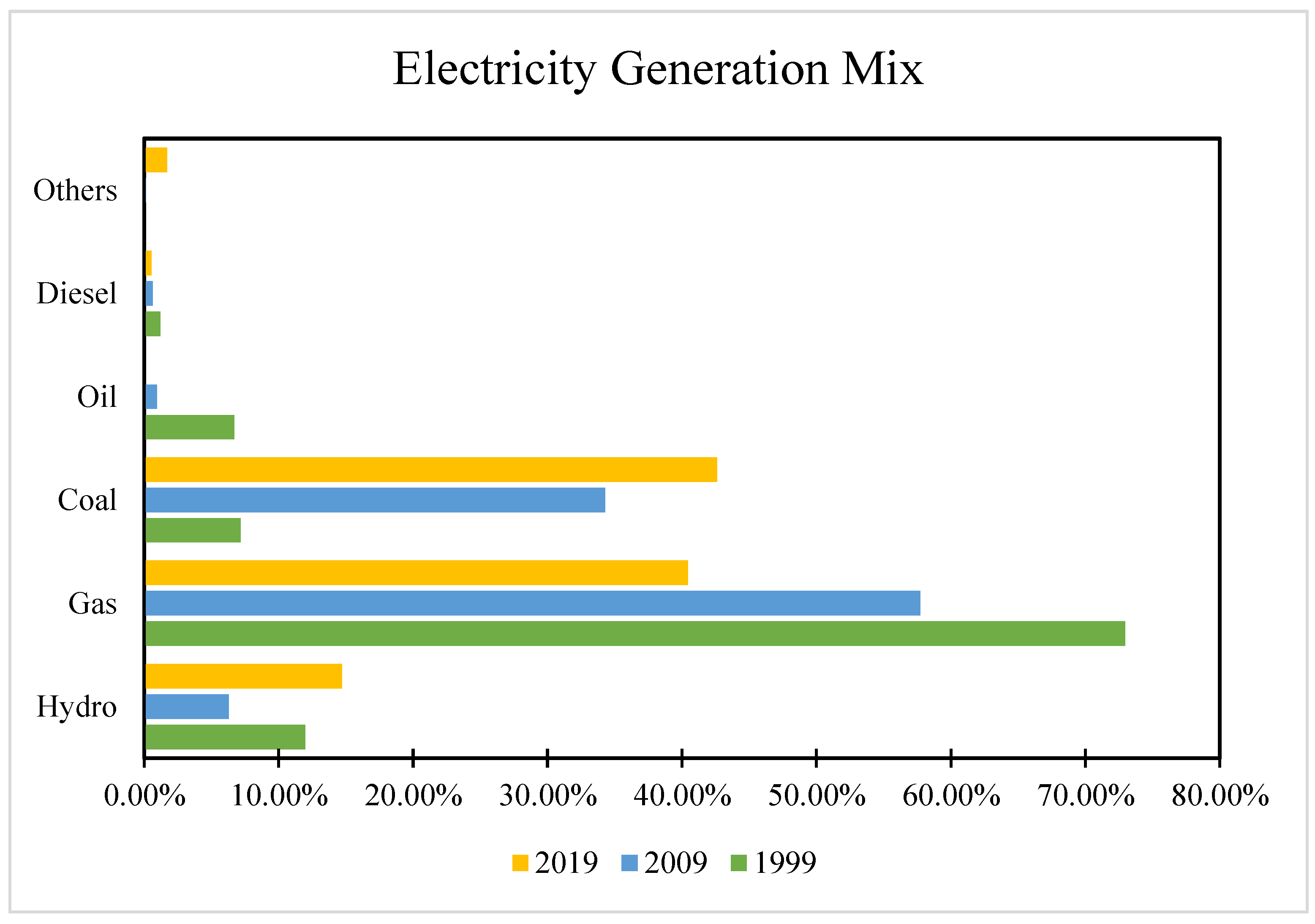In addition, Mohd Yunin, Shabadin, Mohd Zulkifli and Syed Mohamed Rahim [11] remarked that the LED for road lighting should not be installed in areas prone to fog and rain since it leads to glare in the eyes of drivers. Nevertheless, Malaysia’s electricity demand is largely fuelled by gas and coal (refer to Figure 1) and the demand continues to rise for the past three decades [13]. In adition, the electricity’s share of the total energy consumption increased from 17.9% in 1998 to 20.3% in 2018 [13]. Hence, the Ministry of Energy and Natural previously known as the Ministry of Energy, Green Technology and Water targets a reduction of 10% in electricity consumption by 2025 from the energy efficiency sector [14].

The energy price in Malaysia has also been increased as its price or electricity tariff is determined by Tenaga Nasional Berhad (TNB), the only electricity utility company in Peninsular Malaysia and the largest public-listed power company in Southeast Asia. The electricity tariff in Malaysia has been revised three times since 2008, and the latest revision took place in 2014. For street lighting use, there are two types of electricity tariffs; one that includes the maintenance work by TNB, which is currently at the current price of RM0.305/kWh after an increase from RM0.261/kWh, and the other rate that does not include the maintenance cost, which is currently priced at RM0.192/kWh from RM0.164/kWh [15].

With the increased price of energy, the recent development of LED lighting technology, and increased awareness of the encouraging environmental impact of adopting street lighting technology, there is a need to revisit the feasibility of LED for road illumination. To date, the existing literature has not come to an agreement on the need to switch from conventional lighting to LED lighting, as well as aspects regarding the energy, cost, and environmental concerns particularly in the Malaysian context [11,12,16,17]. These three aspects (energy, cost, and environmental concerns) are very crucial in adopting sustainable street lighting technology but lack of clear insights from these different perspectives would hinder the implementation of necessary measures. Therefore, more in-depth study is needed to apprehend the impact of adopting LED for road lighting in Malaysia.

In this light, the purpose of this study is to investigate the performance of LED in substitution for high-pressure sodium vapour (HPSV) road lighting in Penang Bridge, Malaysia using the Data Envelopment Analysis (DEA), a frontier-based optimisation approach, by modelling energy, cost, and environment together. The performance of LED and HPSV road lighting in this study will be measured by the technical efficiency and eco-efficiency of LED and HPSV road lighting. The remainder of this paper is organised into five sections. Section 2 delves into the concept of efficiency in DEA and introduces the theoretical aspect of the variables selected for the optimisation model from the review of the existing literature. We demonstrate our DEA model in Section 3, the efficiency performance analysis of LED and HPSV road lighting in Section 4, and the concluding remarks in Section 5.

2. Literature Review

2.1. Lamp Technologies

A light source is the most significant component of a lighting system because it merely defines visual value, cost, and efficiency of the lighting system [18]. Four important features in light source selection include illumination level required by a particular road according to codes and standards, colour rendering properties of the lamp, lamp lifetime and lamp efficacy [18]. Previously, the high intensity discharge (HID) lighting systems were widely used for road lighting as opposed to incandescent and fluorescent lighting. HPS, LPS, MH and MV lights are classified as the main road lighting technologies of HID lighting systems for road lighting use [19].

Table 1. Characteristics of main road lighting technologies.

Lamp Type	CRI	Luminous Efficacy (lm/W)	Lifetime (Hours)
High-pressure sodium (HPS)	30	50–150	15,000–24,000
Low-pressure sodium (LPS)	5	100–190	18,000–24,000
Metal halide (MH)	70–95	70–130	8000–12,000
Mercury vapour (MV)	50	50	10,000
Light-emitting diode (LED)	70–90	Up to 160	40,000–100,000+

Source: Babatunde, Akinbulire, Oluseyi and Emezirinwune [18].

presents the characteristic of five (5) main road lighting technologies which are HPS, LPS, MH, MV, and LED.

Table 1 compares colour rendering index (CRI) (an index to quantify the ability of a light source to render colour of surfaces accurately), luminous efficacy (a measure of how well a light source can produce visible light), which is measured in lumens per watt (lm/W), and lifetime (the life expectancy until the end-of-life) [18,19,20,21]. MH has the best colour rendering properties, and its luminous efficacy is considerably high, but the lifetime is relatively low. MV consumes high energy, and it also has poor lifetime. Among these HID lighting systems, the HPS lights are the most commonly used for conventional and high mast road lighting due to their excellent luminous efficiency, power usage, and long lifespan [19]. Nevertheless, LED has good CRI and efficacy, and the striking feature of LED is found through its highest lamp lifetime, which is ranging from 40,000 to over 100,000 h.

An HPS lamp commonly composed of four fundamental components, namely a sealed, translucent ceramic arc tube, main electrodes, an outer bulb, and a base. While a basic LED is made up of optical, electrical and mechanical, and thermal components [19,22]. An HPS lamp requires ballasts or capacitors to regulate the arc current flow and deliver the proper voltage to the arc, hence it is powered by an alternating current (AC) source [19]. LEDs utilise an electronic arrangement that converts the supply voltage to low-voltage direct current (DC), making it more energy efficient [18].

2.2. Concept of Efficiency in DEA

Data envelopment analysis (DEA) is a non-parametric approach that measures the performance of decision-making units (DMUs) in a single index value taking multiple inputs and multiple outputs. Pioneered by Charnes et al. [23] and developed from Farrell [24], DEA uses linear programming to estimate relative efficiency, a non-negative value, based on linear relationships between the inputs and outputs of DMUs under analysis. This data-driven performance measurement technique determines how efficient a DMU is in producing a certain level of output, based on the amount of input it uses as compared to other similar DMUs [25]. The Charnes, Cooper and Rhodes (CCR) DEA benchmarking model provides the information by locating and understanding the nature of inefficiencies of a DMU through comparisons with selected efficient DMUs of a similar profile.

Several studies have examined efficiencies in energy by adopting the DEA approach. Ashuri et al. [26] established the DEA energy benchmarking model by taking into account criteria such as total energy usage, building attributes, and local meteorological conditions for a more energy-efficient facility management work. In a large scale, Ervural et al. [27], who employed DEA to analyse renewable energy efficiencies of 81 cities in Turkey, discovered that regions with a high renewable energy potential can turn out to be efficient depending upon their regional technical advancement.

Nevertheless, the conventional efficiency formulation of the DEA tends to improve the performance of inefficient DMUs as soon as the efficient frontier is identified, by either increasing the current level of outputs or decreasing the current level of inputs. In the circumstances when the efficiency can be increased by maximising inputs or the efficiency can be reduced by minimising outputs [28,29]. These are usually referred to as ‘undesirable’ or ‘bad’ input and output variables. The production of ‘undesirable’ by-products such as pollutants and wastes are considered dangerous because of their negative impacts on the environment. Moreover, not considering the production of undesirable outputs in the DEA model development may result in biased efficiency measurement. During the evaluation process of the production performance, particularly when inefficiency exists, the desirable and undesirable outputs should be treated differently in order to improve the inefficiency [30].

There are four common methods to treat undesirable outputs [31]: neglecting undesirable outputs, treating undesirable outputs as inputs, treating the undesirable outputs in the nonlinear model, and applying necessary transformations to the undesirable outputs. An earlier study by Yang and Pollitt [32] showed that enforcing a technically correct disposability features on undesirable outputs makes a substantial impact on the final efficiency evaluation. Zhang et al. [33] established an eco-efficiency analysis on regional industrial systems in China by treating undesirable outputs as inputs. One of the nonlinear models developed for undesirable outputs is the directional distance function (DDF), which has been applied successfully on two separate occasions by Alfredsson et al. [34] and Halkos and Papageorgiou [35].

2.3. Input-Output Variables Selection

2.3.1. Techno-Economic Analysis of Road Lighting System

Techno-economic analysis (TEA) in general is a cost-benefit comparison resulting from the consideration of both technological and economic factors [36]. Zimmermann et al. [37] defined TEA as ‘a methodology framework to analyse the technical and economic performance of a process, product or service and includes studies on the economic impacts or research, development, demonstration, and deployment of technologies’. The TEA approach is used to conduct a cost-benefit analysis by utilising several methodologies to accomplish objectives such as determining the economic feasibility of a particular project, analysing cash flows over the duration of a project’s lifespan, determining the scales and applications of a technology, and comparing the economic quality of various technologies [38].

Net present value (NPV), internal rate of return (IRR), payback period, and return on investment (ROI) are some of the techniques. Several studies have employed these techniques to measure the efficiency of energy-efficient technology through their investments in lighting technology by techno-economic analysis. Yoomak et al. [39], for example, evaluated the performance of their investment in LED lighting to replace HPS road lighting in Thailand using the payback period and IRR. Their findings agreed that LED lighting meets the investment targets and has good potential quality, energy savings, and powerful lighting. Beccali et al. [40] carried out NPV and payback period for the return on investment by considering the on/off control and dimming control of LED retrofit funded through loan, self-funded, and incentive provided by the Italian Government. They found that LED retrofits with dimming control funded through the incentive provided by the Italian Government give the highest NPV value and a return time of 4 to 5 years.

There are two important types of cost to be considered in analysing the investment made on road lighting technology, namely the initial investment cost and operating cost. The initial investment cost is the installation cost [41], and this is one of the important aspects to consider in adopting LED lighting technology [42]. The fact that price of LED lighting is much higher compared to the conventional lighting, LED lighting systems would require a higher initial investment cost [43,44], which then could result in a low penetration rate of LED lighting.

The other fundamental segment of road lighting costing is the operation cost. Operation cost comprises energy consumption and maintenance cost. While the energy price makes up the consumption cost, the maintenance cost consists of the cost of cleaning and upkeeping of the lanterns [45,46]. Therefore, economic feasibility of the streetlight depends heavily on electricity prices [47], as revealed by Duman and Güler [48]. Meanwhile, Beccali et al. [49] found that the annual capital savings on a new LED lighting system could be attributed to maintenance cost and reduction in energy consumption.

2.3.2. Energy Consumption

Energy saving and efficiency have received high affinity among researchers specifically in road lighting installation. The literature on energy savings and efficiency for road lighting installation is analysed in three aspects, namely by optimising the design of road lighting system with the best parameter combination to ensure lighting regulating and installation efficiency, improving lamp and luminaire technology, and improving lamp and luminaire control systems [4,5,50]. Owing to these efforts, more sustainable road lighting technology has been developed and improved [2]. Previous studies also associated reduced energy consumption to energy savings with new LEDs’ design status. Djuretic and Kostic [51], for instance, underlined the need to choose similar photopic or mesopic luminance levels and they found that the high-quality LED luminaires could save 31 to 60% of energy as compared to the high-quality HPS luminaires applicable to multi-stage scenarios. Yoomak, Jettanasen, Ngaopitakkul, Bunjongjit and Leelajindakrairerk [39], on the other hand, studied power quality and energy savings of LED road lighting from the DIALux simulation programme, where the energy efficiency index difference was approximately 40%.

In a study on pedestrian street lighting, Juntunen et al. [52] developed smart LED luminaires with higher luminous efficacy to demonstrate energy savings without sacrificing user visual comfortability. In the passive mode, where the streetlights function without added intelligence, energy savings of 19 to 44% were achieved as compared to commercial luminaires. There is also huge potential for power consumption reduction in the LED lighting system with a control system [53,54]. Energy savings without comprising user visual comfortability has achieved a reduction of 38% energy consumption in an indoor experiment on the control of SPDs of LED lighting [55].

Pipattanasomporn, Rahman, Flory and Teklu [54] found that an intelligent lighting control system may reduce approximately 74% of energy usage. On the other hand, Bunjongjit, Ananwattanaporn, Ngaopitakkul, Jettanasen and Patcharoen [53] proposed a control circuit for LED luminaire based on the amount of daylight which has been able to reduce the lighting system’s power consumption while preserving lighting quality for the user. Smart Grid technology equally has the potential to further increase the efficiency and operational reliability of outdoor lighting systems as discussed by Filimonova et al. [56] on an LED outdoor lighting system for a university campus in Russia.

2.3.3. Lifetime of the Luminaire

Lifetime is the useful life of luminaire. LED advances have resulted in significant improvements in light source efficiency and lifetime [57]. In the market, the lifetime of LED lights involving LED drivers and source packages is regularly quoted as 25,000 to 50,000 h [58,59,60,61]. In general, the lifetime of LED lights is two to six times more than conventional lights which will reduce maintenance costs [49]. Nonetheless, poorly designed LED driver and high temperatures might shorten the lifetime of LED lights [62,63].

2.3.4. Environmental Concern in Road Lighting System

The assessment of environmental impact is the other well-researched topic in LED road lighting. Tannous et al. [64] utilised life cycle assessment (LCA) in measuring environmental impact to compare the usage of solar-LED and traditional-HPS road lighting. They considered LCA from the raw material extraction until the end-of-life, with two end-of-life scenarios modelled, landfilling and recycling. They concluded that the solar system has fewer overall environmental impacts than the traditional system for both landfilling and recycling scenarios. Many others looked into carbon dioxide emission reduction when assessing the environmental impact of the LED and conventional LED for road lighting illumination [4,18,44,48,49]. Carbon dioxide emission can be computed directly from electricity consumption by applying the multiplication of the carbon dioxide emission factor of a country.

3. Materials and Methods

3.1. Techno-Economic Analysis (TEA)

This study specifically applies the TEA techniques, which include payback period, cash flow, net present value (NPV), internal rate of return (IRR), and return on investment (ROI). Discount rates of 5% and 10% are also being considered [39,65].

NPV is defined as the sum of the present value of all cash flow produced by the project, comprising the investment cost; and if the value of NPV is positive, the investment is acceptable to proceed [43,66]. The NPV formulation is shown in Equation (1).

$$\mathrm{NPV}={\displaystyle \sum }_{t=0}^{n-1}\frac{I_t}{{\left(1+i\right)}^t}+{\displaystyle \sum }_{t=1}^n\frac{N{R}_t}{{\left(1+i\right)}^t}$$

(1)

where $I_t$ is the investment cash-flow in period t, $N{R}_t$ is the net revenue in period t, $i$ is the discount rate, and $n$ is the number of years. Next, IRR is the discount rate, which equalised NPV to zero, and the IRR value must be greater than the investment cost for the project to be accepted [43,66]. The IRR formulation is shown in Equation (2).

$$0={\displaystyle \sum }_{t=0}^{n-1}\frac{I_t}{{\left(1+\mathrm{IRR}\right)}^t}+{\displaystyle \sum }_{t=1}^n\frac{N{R}_t}{{\left(1+\mathrm{IRR}\right)}^t}$$

(2)

ROI is the ratio of the present value of cash flow and the investment [43,66]. An ROI that is greater than one (1) indicates that the investment is profitable and worthwhile [65]. ROI is presented in Equation (3).

$$\mathrm{ROI}={\displaystyle \sum }_{t=1}^n\frac{N{R}_t}{{\left(1+i\right)}^t}/{\displaystyle \sum }_{t=0}^{n-1}\frac{I_t}{{\left(1+i\right)}^t}$$

(3)

Payback period can be defined as the period of time required to recover the investments [43,66]. The payback period is shown in Equation (4).

$$\mathrm{Payback} \mathrm{Period}={\displaystyle \sum }_{t=0}^{n-1}\frac{I_t}{{\left(1+i\right)}^t}/{\displaystyle \sum }_{t=1}^n\frac{N{R}_t}{\left(\frac{{\left(1+i\right)}^t}{n}\right)}$$

(4)

A simple payback period and discounted payback period were investigated in this study. This is crucial as a simple payback period does not consider the time value of the money or all the cash flows. Hence, the discounted payback period overcomes the weakness of the simple payback period. The NPV, IRR, ROI and payback period are obtained by using Microsoft Excel computation.

3.2. Data Envelopment Analysis (DEA)

This study utilised the DEA approach mainly due to its benchmarking capabilities and characteristics that may consist of multiple inputs and multiple outputs. This study considers energy, cost, and environmental concerns in a single model. The Charnes, Cooper and Rhodes (CCR) of the DEA model is shown in Section 3.2.1. Nevertheless, the conventional DEA model only accounts for two categories of variables, which are the input, and the desirable output variables. As discussed earlier, the presence of undesirable output such as the carbon dioxide emission in the conventional DEA model should not be neglected. To incorporate undesirable outputs for measuring efficiency, a recognized Directional Distance Function (DDF) approach is employed. This technique is able to evaluate the eco-efficiency of LED road lighting usage and the DDF model is presented in Section 3.2.2.

3.2.1. CCR of DEA Model

The linear programming problem of the input-oriented CCR model is given as follows for the $p$-th DMU $\left({\mathrm{DMU}}_{\mathrm{p}}\right)$ under consideration:

$$\begin{gathered} {\theta }^{\ast }=\min \theta \\ \mathrm{subject} \mathrm{to} \\ {\displaystyle \sum }_{k=1}^K{z}_k{x}_{kn}\le \theta x_{np}; n=1,\dots ,N \\ {\displaystyle \sum }_{k=1}^K{z}_k{y}_{km}\ge y_m;m=1,\dots ,M \\ {z}_k\ge 0 ; k=1,\dots ,K \end{gathered}$$

(5)

where $x_n$ represents the n-th input, $y_m$ represents the m-th output of a DMU, and $z_k$ are the intensity variables or weights assigned to each K DMUs involved. The total number of inputs and outputs are represented by N and M with N and M > 0.

In this study, three inputs, and one desirable output are considered for ten DMUs to measure the technical efficiency score ${\theta }^{\ast }$. Therefore, let the total number of inputs and outputs be represented by N = 3 and M = 1, and the number of DMU is represented by K = 10. From Equation (5), the linear programming problem of the CCR model to minimise the inputs for a specific $p$-th DMU is given by

$$\begin{gathered} {\theta }^{\ast }=\min \theta \\ \mathrm{subject} \mathrm{to} \\ {\displaystyle \sum }_{k=1}^{10}{z}_k{x}_{kn}\le \theta x_{np}; n=1,2,3. \\ {\displaystyle \sum }_{k=1}^{10}{z}_k{y}_{km}\ge y_m;m=1. \\ {z}_k\ge 0 ; k=1,\dots ,10. \end{gathered}$$

(6)

In Equation (6), variable $x_1$ denotes the input variable of installation cost, variable $x_2$ denotes the input variable of operation cost, variable $x_3$ denotes the input variable of energy consumption, and variable $y_1$ denotes the desirable output variable of lifetime. Further explanation on the input and output variables is available in Section 3.3. Hence, let the DMU1 be an example for Equation (6). The technical efficiency score ${\theta }^{\ast }$ for DMU1 is given by

$$\begin{gathered} {\theta }^{\ast }=\min \theta \\ \mathrm{subject} \mathrm{to} \\ {\displaystyle \sum }_{k=1}^{10}{z}_k{(\mathrm{installation} \mathrm{cost})}_k\le \theta {\left(\mathrm{installation} \mathrm{cost}\right)}_1 \\ {\displaystyle \sum }_{k=1}^{10}{z}_k{\left(\mathrm{operation} \mathrm{cost}\right)}_k\le \theta {\left(\mathrm{operation} \mathrm{cost}\right)}_1 \\ {\displaystyle \sum }_{k=1}^{10}{z}_k{\left(\mathrm{energy} \mathrm{consumption}\right)}_k\le \theta {\left(\mathrm{energy} \mathrm{consumption}\right)}_1 \\ {\displaystyle \sum }_{k=1}^{10}{z}_k{\left(\mathrm{lifetime}\right)}_k\ge \left(\mathrm{lifetime}\right) \\ {z}_k\ge 0 ; k=1,\dots ,10 \end{gathered}$$

(7)

There are ten equations similar to Equation (7) constructed for each DMU to obtain the technical efficiency score ${\theta }^{\ast }$. In this input-oriented model, the efficiency of a DMU measurement involves an effort of minimising θ, producing the observed outputs within minimum input [29]. Here, we can assess the performance of DMUs from a benchmarking perspective, by identifying which DMU is efficient, and which is not. The inefficient DMU can further be improved based on the information obtained by comparing it with the efficient DMU.

DEA assessment establishes the ‘best’ or ‘efficient’ rather than average behaviour [67]. The best performing DMU is allocated with an efficiency score of 100 percent, while the performance of other DMUs may vary between 0 and 100 percent relative to the best performance [29,67]. In addition, both input-oriented and output-oriented measurements offer the same results of relative efficiency scores under constant returns to scale but contribute to different values under variable returns to scale [68,69].

3.2.2. DDF of DEA Model

The DDF approach is an evaluation technique that estimates relative efficiency of a decision-making unit (DMU) along a pre-determined direction vector that is not restricted by the radial direction. The DDF is used to measure eco-efficiency of the ${\mathrm{DMU}}_p$ under constant returns to scale and weak disposability of undesirable output assumptions:

$$\begin{gathered} \max {\beta }_p \\ \mathrm{subject} \mathrm{to} \\ {\displaystyle \sum }_{k=1}^K{z}_k{x}_{kn}\le x_n; n=1,\dots ,N \\ {\displaystyle \sum }_{k=1}^K{z}_k{y}_{km}\ge y_m\left(1+{\beta }_p\right); m=1,\dots ,M \\ {\displaystyle \sum }_{k=1}^K{z}_k{u}_{ki}=u_i\left(1-{\beta }_p\right); i=1,\dots ,I \\ {z}_k\ge 0; k=1,\dots , K \end{gathered}$$

(8)

The inefficiency score of the ${\mathrm{DMU}}_p$ is given by $0\le {\beta }_p\le 1$ for the undesirable outputs involved. A score of zero denotes an efficient DMU while a score of any positive value indicates inefficiency. This study has three inputs, one desirable output, and one undesirable output that are considered for ten DMUs. Therefore, the total number of inputs and outputs is represented by N = 3, M = 1 and I = 1, and the number of DMU is represented by K = 10. From Equation (8), the linear programming problem of the DDF model to measure inefficiency for a specific $p$-th DMU is given by

$$\begin{gathered} \max {\beta }_p \\ \mathrm{subject} \mathrm{to} \\ {\displaystyle \sum }_{k=1}^{10}{z}_k{x}_{kn}\le x_n; n=1,2,3 \\ {\displaystyle \sum }_{k=1}^{10}{z}_k{y}_{km}\ge y_m\left(1+{\beta }_p\right); m=1 \\ {\displaystyle \sum }_{k=1}^{10}{z}_k{u}_{ki}=u_i\left(1-{\beta }_p\right); i=1 \\ {z}_k\ge 0; k=1,\dots , 10 \end{gathered}$$

(9)

In Equation (9), variable $x_1$ denotes the input variable of installation cost, variable $x_2$ denotes the input variable of operation cost, variable $x_3$ denotes the input variable of energy consumption, variable $y_1$ denotes the desirable output variable of lifetime, and variable $u_1$ denotes the undesirable output of carbon dioxide emissions. Further explanation on the input and output variables is available in Section 3.3. Hence, let the DMU1 be an example for Equation (10). The inefficiency score $\beta$ for DMU1 is given by

$$\begin{gathered} \max {\beta }_1 \\ \mathrm{subject} \mathrm{to} \\ {\displaystyle \sum }_{k=1}^{10}{z}_k{\left[\mathrm{installation} \mathrm{cost}\right]}_k\le \left[\mathrm{installation} \mathrm{cost}\right] \\ {\displaystyle \sum }_{k=1}^{10}{z}_k{\left[\mathrm{operation} \mathrm{cost}\right]}_k\le \left[\mathrm{operation} \mathrm{cost}\right] \\ {\displaystyle \sum }_{k=1}^{10}{z}_k{\left[\mathrm{energy} \mathrm{consumption}\right]}_k\le \left[\mathrm{energy} \mathrm{consumption}\right] \\ {\displaystyle \sum }_{k=1}^{10}{z}_k{\left[\mathrm{lifetime}\right]}_k\ge \left[\mathrm{lifetime}\right]\left(1+{\beta }_1\right) \\ {\displaystyle \sum }_{k=1}^{10}{z}_k{\left[CO2 \mathrm{emissions}\right]}_k=\left[CO2 \mathrm{emissions}\right]\left(1-{\beta }_1\right) \\ {z}_k\ge 0; k=1,\dots , 10 \end{gathered}$$

(10)

There are ten equations similar to Equation (10) constructed for each DMU to obtain the inefficiency score $\beta$ for ten DMUs. This is followed by computing the eco-efficiency score $\partial$. The eco-efficiency score $\partial$ using the DDF model from the inefficiency score in Equation (9) for the ${\mathrm{DMU}}_p$ is given by the following:

$${\partial }_p=1-{\beta }_p$$

(11)

Note that $0\le {\beta }_p\le 1$, thus $0\le {\partial }_p\le 1.$ Therefore, the eco-efficiency score $\partial$ for DMU1 is given by the following:

$${\partial }_1=1-{\beta }_1$$

(12)

Note that $0\le {\beta }_1\le 1$, thus $0\le {\partial }_1\le 1.$ The eco-efficiency score $\partial$ is also calculated for other DMUs evaluated in this study (DMU2 to DMU10).

3.3. Specification of Variables Selection

3.3.1. Determination of Research Area and Decision-Making Unit (DMU)

The Penang Bridge highway is the study area to compare the HPSV and LED lighting technology where retrofitting of the lanterns took place as such lighting parameters (lighting class, type of carriageway, lighting arrangement, total distance illuminated, spacing between lighting pole, and number of light poles) and components of a road lighting pole (mounting height, overhang, boom angle and boom length) remain constant. The DMU of this study is the two types of lanterns positioned near five metering points along the Penang Bridge. Therefore, there are five DMUs for each type of lighting technology, making it a total of ten DMUs under study.

3.3.2. Determination of Input and Output Variables

There are several suggestions to determine the number of input and output variables to be included in the DEA modelling [70,71,72]. Nevertheless, the suggestions are often imposed for convenience and do not have a statistical basis and are not crucial to be fulfilled [73]. It is unnecessary to apply a sample size requirement to DEA because DEA is a frontier-based linear programming-based optimisation technique, and it is also essential to include as many relevant inputs and outputs as possible [73].

In this study, there are three input variables: installation cost, operation cost, and energy consumption, and two outputs: a desirable lantern’s lifetime and undesirable carbon dioxide (CO₂) emission. This study focused on undesirable outputs rather than undesirable inputs with the aim to include the environmental factor of carbon dioxide emission as the by-product from the energy consumption of road lighting in the model development [4,65,74].

Table 2. List of variables.

Variable	Name of Variable	Definition	Unit Measurement
Input	Installation cost ($x_1$)	The cost of installing lighting fixture including labour [19,45]	RM
	Operation cost ($x_2$)	The cost includes electricity consumption cost and maintenance cost [46]	RM
	Energy consumption ($x_3$)	The actual electricity consumption for all road lightings in Penang Bridge	kWh
Desirable output	Lantern’s lifetime ($y$)	The life expectancy until the end-of-life [21]	Hours
Undesirable output	Carbon dioxide (CO2) emission ($u$)	The by-product from the road lighting usage as the environmental analysis [4]	kg CO2 per kWh

below provides a summary of the input and outputs used in this study, together with the definition and the unit of measurement.

3.3.3. Data Source

Two types of lighting technology, HPSV and LED, are being compared in this study. Hence, all data for this study were obtained from PLUS Malaysia Berhad, the largest highway concessionaries company in Malaysia. The data for CO₂ emissions are calculated by utilising the carbon dioxide emission factor of 0.6931 kg CO₂-e/year associated to each kWh of electricity generated HPSV and LED road lightings based on Ang and Su [75].

Table 3. Descriptive Statistics of Input and Outputs for HPSV and LED Road Lighting.

Type of Lighting		Input			Output
		Installation Cost (RM)	Operation Cost (RM)	Energy Consumption (kWh)	Carbon Dioxide (CO2) Emission (kg per kWh)
HPSV	Mean	120,291.00	36,539.71	62,085.8000	43,031.6680
	Standard deviation	75,231.61	24,124.29	38,830.5775	26,913.4733
	Maximum	32,3417.14	246,069.83	76,210.3600	12,7003.0000
	Minimum	67,472.87	52,633.79	14,595.8900	27,152.0000
LED	Mean	171,901.00	21,042.56	43,682.8000	30,276.5487
	Standard deviation	113,721.4873	10,123.67	29,909.0500	20,729.9625
	Maximum	368,598.82	37,657.15	95,568.0000	66,238.1808
	Minimum	86,815.76	11,865.79	21,608.0000	14,976.5048

provides the descriptive statistics of the input and output dataset employed in this study.

For each type of HPSV and LED road lighting on the Penang Bridge, five DMUs are being evaluated based on its technical efficiency and eco-efficiency by using Rstudio software. The following section presents the results and empirical findings.

4. Results and Discussion

This section demonstrates the empirical findings from the Techno-Economic Analysis (TEA) and Data Envelopment Analysis (DEA) approach which help to give some insights into the performance of HPSV and LED road lighting in the Penang Bridge highway.

4.1. The NPV, IRR, ROI, Cash Flow, and Payback Period

This section describes the findings from the analysis on NPV, IRR, ROI, cash flow, and payback period. The lantern lifetime in the unit of year was computed to project the number of lanterns for the period of 11 years and the results are presented in

Table 4. Number of lanterns required for 11 years between HPSV and LED lanterns.

Lantern Type	HPSV	LED
Power rating (W)	400	230
Lifespan based on specification (hour)	20,000	50,000
Operating hours per day (hour)	12	12
Lifetime (year)	4.56	11.42
The ratio of lanterns required for 11 years	2.41	0.96
	3	1
Number of lanterns required for 11 years	1191 units	397 units

.

From Table 4, at a daily usage of 12 h and an expected lifetime of 50,000 h, an LED lantern could last for approximately 11.42 years, while an HPSV lantern with an expected lifetime of 20,000 h could only last for 4.56 years. For the projected 11 years of implementation, the projected number of HPSV and LED lanterns to be acquired are 1191 and 397, respectively; that is HPSV lanterns require three times more replacement as compared to LED lanterns. In consequence, the installation cost for the implementation of LED lanterns would be much lower than HPSV lighting. More importantly, with a smaller number of more environmentally friendly lanterns to be implemented, the concentration of carbon dioxide emission can be reduced to a great extent for a period of 11 years. The implementation of LED lighting technology for road lighting promotes sustainable practices through the smart use of energy that not only meets the present needs, but also conserves them for future necessities.

Table 5. Investment cost of LED lanterns.

Parameter	Value
Initial investment cost of LED lantern (RM)	859,505.00
Annual electricity cost—LED (RM/year)	216,232.58
Annual electricity cost—HPSV (RM/year)	394,110.10
Cost of lantern replacement—HPSV (RM/year)	132,327.25
Annual saving (RM/year)	310,204.76
Simple payback period (year)	2.77

summarises the costs related to the investment in HPSV and LED lanterns and the period of analysis for the investment made was assumed at 11 years, based on the findings from Table 4.

Table 5 reports the investment in LED lanterns. Annual saving is obtained by adding the annual electricity cost and replacement cost of HPSV lighting, then subtracting it from the annual electricity cost of LED lighting. Hence, the annual saving on replacing HPSV with LED lanterns is RM310,204.76 per year. By dividing the investment cost of LED lanterns by annual savings, the simple payback period for LED lantern replacement is 2.77 years. 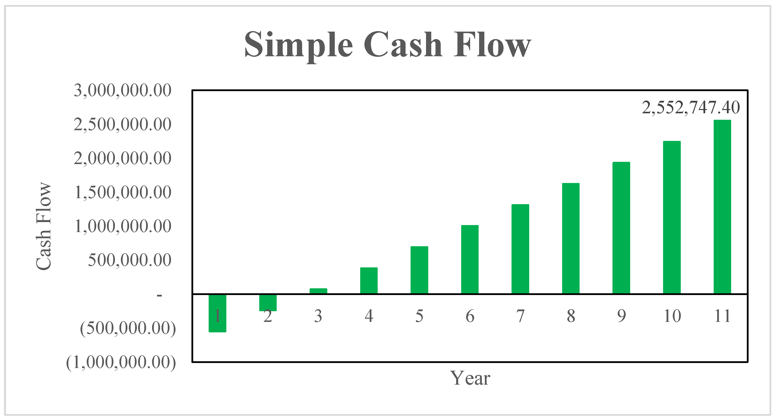Therefore, the investment cost to be paid in the eighth month of the third year is as portrayed in Figure 2. A simple cash flow from the investment in LED lanterns made for the 11-year period is shown in Figure 2 as below:

Figure 2 illustrates the negative values of cash flow representing the amount of investment made while the positive values represent the savings obtained. The first two years are the early phase of the LED adoption, which involves a large amount of investment in purchasing and installation of new lanterns. As such, Figure 2 depicts a negative cash flow because the investment needs a period of recovery before the return of investment can be achieved. From the third year onwards, positive trends are observed as the investment starts to contribute positive income through the savings from the replacement of HPSV with LED lanterns. Hence, in the eleventh year, the positive income obtained is RM2,552,747.40. In a total duration of eleven years, nine years of positive income can be preserved before the next phase of LED lantern replacement.

Information in Table 5 was further used to calculate the NPV, IRR, ROI, and discounted the payback period. The results are reported in

Table 6. Results of TEA.

Parameter	Value at 5% Discount Rate	Value at 10% Discount Rate
Net present value (RM)	1,717,184.26	1,155,293.86
Internal rate of return (%)	34.73	34.73
Return on investment	1.08	1.08
Discounted payback period (year)	3.06	3.42

, where discount rates of 5% and 10% are considered [39,65].

From the results in Table 6, at a 5% discount rate, an investment of RM859,505.00 generates an NPV of RM1,717,184.26, an IRR of about 34.73%, and an ROI of about 1.08. The discounted payback period for this investment is 3.06 years. As the discount rate increases to 10%, the same amount of investment on LED lanterns will decrease the NPV to RM1,155,293.86, maintaining IRR and ROI at 34.73% and 1.08, respectively, and increases the discounted payback period to 3.42 years. NPV is at positive rates of 5% and 10% discount. Hence, the utilisation of LEDs for road lighting should be able to proceed due to the positive NPV even though a higher discount rate has been used.

A positive NPV indicates that the investment has a positive cash flow, in this case, results in savings. Additionally, an IRR of 34.73% for both 5% and 10% discount rate can be used as a reference to future ranks of LED lighting projects since it is a powerful evaluation index for investigating the profitability of projects. A total of 34.73% of IRR suggests that the probability of getting a profitable investment is almost as high as 35%. As the ROI is 1.08 or 108%, it suggests that RM1.08 is obtained for every Malaysian Ringgit (MYR) value of investment made on LED lanterns, and the range of 3 to 4 years is required to recoup the investment.

4.2. Technical Efficiency

This section illustrates the results using the DEA approach under the constant returns to scale (CRS) assumption on technology of the CCR model. This technical efficiency accounts for input variables (investment cost, operation cost, and energy consumption) and desirable output (lantern’s lifetime). The technical efficiency score ${\theta }^{\ast }$ is acquired from Equation (6) in Section 3.2.1. The results of the technical efficiency scores and ranks are presented for HPSV and LED road lighting in the Penang Bridge highway according to the type of road lighting technology. The average efficiency score for each type of road lighting is calculated to determine a summary of the road lighting technical efficiency. The technical efficiencies and ranks using the DEA model with CRS assumptions for HPSV and LED road lighting in the Penang Bridge highway together with the most important input variables are presented in

Table 7. Results of the DEA technical efficiency score, rank, and the most important input variables for HPSV and LED Road Lighting.

Metering Point	$\mathbf{Technical} \mathbf{Efficiency} \mathbf{Score} {\mathit{\theta }}^{\ast }(\%)$	Rank	The Most Important Input Variable
HPSV1	37.19	7	Installation cost
HPSV2	14.11	10	Installation cost
HPSV3	42.36	6	Installation cost
HPSV4	65.98	3	Installation cost
HPSV5	27.26	9	Installation cost
Average efficiency score	37.38
LED1	83.76	2	Installation cost
LED2	31.69	8	Operation cost
LED3	54.16	5	Installation cost
LED4	100	1	Installation cost
LED5	61.94	4	Installation cost
Average efficiency score	66.31
Total average efficiency score	51.85
Number fully efficient	1

.

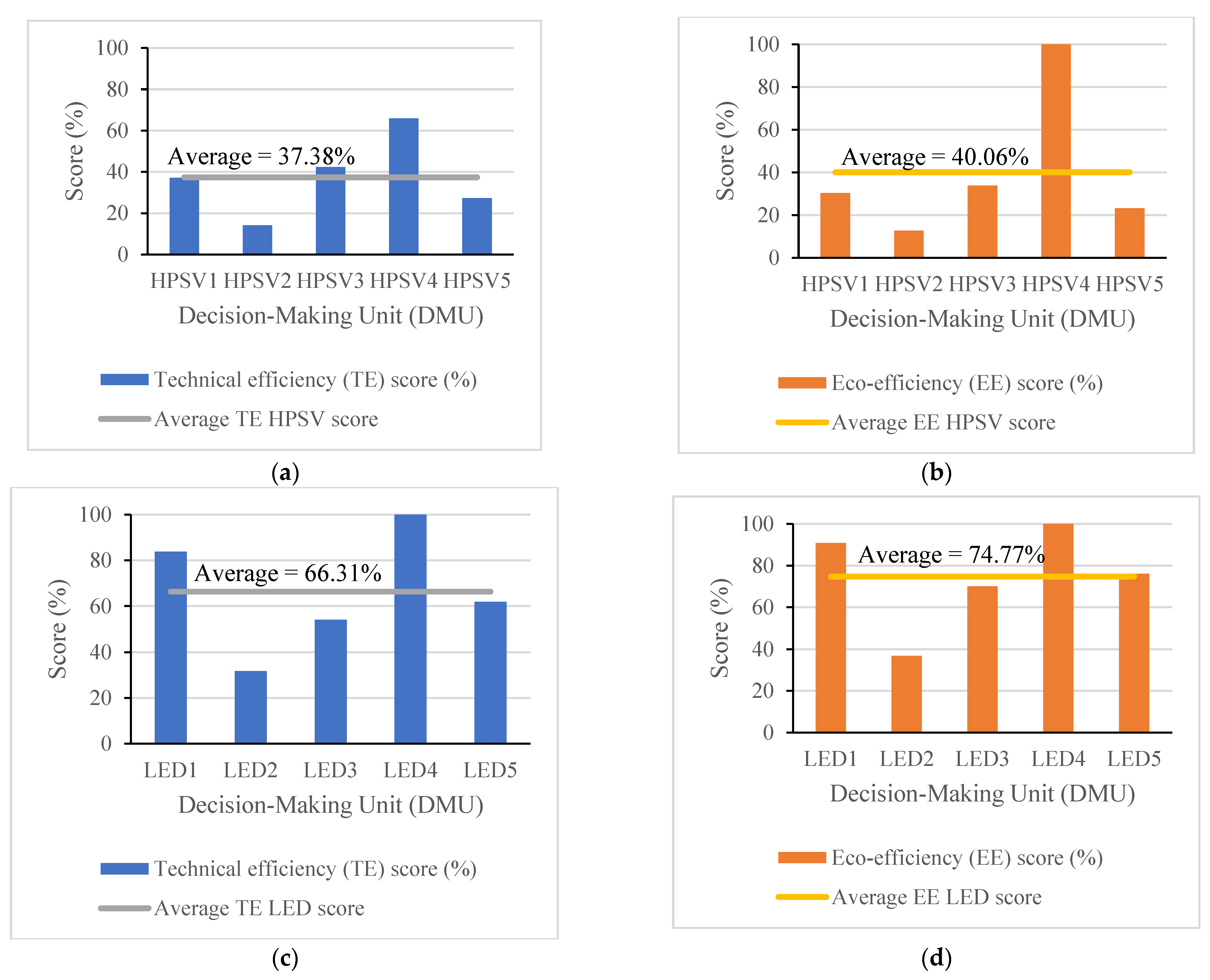
From Table 7, there are nine DMUs with scores less than 100% that are regarded as inefficient. Inefficient scores are ranging from 14.11% to 83.76% and the only technical efficient or fully efficient DMU with a 100% score is LED4. LED2 ranked in the eighth place, out of ten, with a score of only 31.69%, while the other DMUs scoring lower than three HPSV road lighting technologies (HPSV4, HPSV3, HPSV1). This exhibits that LED2 does not utilise the input resources appropriately during its operation. Hence, it performs poorer than the conventional road lighting technology of HPSV.

In addition, the performance of DMU of HPSV4 is as good as LED5 and LED3, with scores of 65.98%, 61.94%, and 54.15%, respectively. One of the possible reasons for this finding is the less economical performance of LED lighting compared to the HPSV lighting. Tähkämö, Räsänen and Halonen [46] found that although LED technology offers improved colour characteristics and lighting controls as compared to high-intensity discharge (HID) lights such as High-Pressure Sodium (HPS), HPS is more economical as compared to LED. As there are two input variables related to cost utilised in this study, the good performance of HPSV4 is not surprising.

Additionally, in the last column of Table 7, it is found that for each evaluated DMU, the installation cost is the most important item in evaluating the performance of road lighting technology for this study except of LED2. It is because the DMU of LED2 demonstrates that the operation cost is the most important item in evaluating its performance. Therefore, with the inefficient score of 31.69%, LED2 could potentially reduce its operation cost by approximately 68.31%.

As mentioned in Section 3.3.2, there are two important components of operation cost, namely electricity consumption cost and maintenance cost. The maintenance cost is influenced by the maintenance work done on the lanterns. According to PLUS Malaysia Berhad [45], as LED technology is still new for the study site, the need for maintenance work such as the cleaning of the optics remains uncertain.

The other aspect of operation cost is the electricity consumption cost which is dependent upon on the electricity or energy consumption and the electricity tariff. Although it can be observed that there is a decrease in energy usage (based on Table 3) by adopting LED lighting technology in Penang Bridge, none of the DMUs reflects the significance of energy consumption in deriving the technical efficiency scores. In addition, there are no changes in the electricity tariff during the study period. Hence, there is no evidence of electricity consumption cost contributing towards the operation cost at that point of time.

The installation cost of LED, however, are found and known to be higher than the conventional road lighting technology [4,76,77,78], and, at the same time, the LED prices have continued to reduce due to the estimated 38 billion total sales of LED lighting products over the last five years [57]. Therefore, it can be observed that two DMUs from LED lighting technology (LED4 and LED1) ranked in the first and second place, surpassing HPSV lighting technology. Still, the DMU of HPSV4 positioned in the third-rank. Thus, a future study can investigate the competitiveness of the current LED price as compared to the HPSV price as this is considered the limitation of this study.

In a DEA convention, a group of fully efficient DMUs serves as reference peers. From Table 7, it can be observed that the only fully efficient DMU is LED4. Therefore, all inefficient DMUs have only one reference peer which is LED4. This indicates that for all evaluated DMUs to operate efficiently, their performance must be improved to operate similarly to LED4.

However, again, the mean efficiency score of LED road lighting technology is 66.31%, which is two times higher than the HPSV road lighting, with only 37.38%. This reflects that the efficiency of road lighting on the Penang Bridge highway has been improved with the adoption of LED technology. The inefficient scores in Table 7 further suggest the possible extent to which certain point inputs could be minimised while maintaining the existing outputs. The excellency and deficiency among the DMUs in this study is simply a relative relationship based on input and output components.

4.3. Comparing Technical Efficiency Groups Test

This section aims to compare the technical efficiency scores of HPSV and LED road lighting. To validate the difference in technical efficiency scores between HPSV and LED, a non-parametric Wilcoxon Signed-Rank Test is utilised, and

Table 8. The Wilcoxon Signed-Rank Test of technical efficiency score for HPSV and LED Road Lighting.

Test Statistics	Wilcoxon Signed-Rank Test
	Mean Rank	z	Sig.
LED to HPSV	3.00	−2.023	0.043

presents the results.

As the results in Table 8 show a p-value of less than 0.05 (p < 0.05), it can be concluded that there is a statistically significant difference in the technical efficiency scores between HPSV and LED road lighting.

4.4. Eco-Efficiency

The eco-efficiency using the DEA model accounts for input variables (investment cost, operation cost, and energy consumption), desirable output (lantern’s lifetime), and undesirable output (carbon dioxide emissions). The eco-efficiency score using the DDF approach is acquired from Equation (11) in the methodology section. The results of the eco-efficiency scores and ranks are presented for HPSV and LED road lighting in the Penang Bridge highway. The average efficiency score for each type of road lighting is calculated in order to determine the eco-efficiency of road lightings. With CRS assumptions for HPSV and LED, the DDF eco-efficiencies are presented in

Table 9. Results of the DEA eco-efficiency score and rank for HPSV and LED Road Lighting.

Metering Point	Score (%)	Rank
HPSV1	30.41	8
HPSV2	12.74	10
HPSV3	33.92	7
HPSV4	100	1
HPSV5	23.24	9
Average eco-efficiency score	40.06
LED1	90.81	3
LED2	36.88	6
LED3	70.03	5
LED4	100	1
LED5	76.14	4
Average efficiency score	74.77
Total average efficiency score	57.42
Number fully efficient	2

.

The eco-efficiency scores in Table 9 show the level of undesired output reduction. For instance, the DMU of LED1 was 90.81% efficient. This finding suggests that LED1 could decrease its undesirable output by 9.19% to achieve full efficiency. In addition, it can be observed that the DMU of HPSV1 and HPSV3 have almost the same performance as LED2, with the scores of 30.41%, 33.92%, and 36.88%, respectively.

Additionally, the HPSV road lighting technology DMUs are the most eco-inefficient DMUs, ranked in the seventh place and below, except for the DMU of HPSV4 which ranked in the first place, together with LED4. It means that, as compared to other DMUs in this study, the DMU of LED4 and HPSV4 are the most eco-efficient DMUs. This shows that HPSV road lighting can perform as good as LED lighting technology when energy, cost, and environmental concerns are considered altogether in the model.

The eco-efficiency scores are quite similar to the technical efficiency scores for all HPSV DMUs except for the DMU of HPSV4. HPSV4 is ranked at third by technical efficiency score and rises to first by eco-efficiency score. This shows the importance of the environmental variable in the model as when the carbon dioxide emission variable is included in the model; the result demonstrates that HPSV lighting technology is able to perform as good as LED lighting technology. This finding supports the findings by Tähkämö and Halonen [17] from their environmental performance assessment using life cycle assessment (LCA) of road lighting. Although they found that the environmental performances of the HPS and LED luminaires are on the same level during the study period, none of the previous studies has included energy, cost, and environmental concern altogether in one model.

The average eco-efficient score for LED road lighting technology is 74.77%, and this is way above the performance of the HPSV road lighting, which is only at 40.06%. Our finding concurs with the findings of Khan and Abas [79] who support LED luminaires that are being recognised as environmentally efficient solutions for roadway lighting [47].

4.5. Comparing Eco-Efficiency Groups Test

This section aims to compare the eco-efficiency scores of HPSV and LED road lighting by performing the non-parametric (Wilcoxon Signed-Rank Test) test.

Table 10. The Wilcoxon Signed-Rank Test of eco-efficiency score for HPSV and LED Road Lighting.

Test Statistics	Wilcoxon Signed-Rank Test
	Mean Rank	z	Sig.
LED to HPSV	2.5	−1.826	0.068

presents the results.

The results in Table 10 show the results of the Wilcoxon signed-rank test, where the p-value of 0.068 is more than 0.05 (p > 0.05). However, as p < 0.10, it can be still concluded that the eco-efficiency scores between HPSV and LED road lighting are still statistically different but at the 10% significance level.

4.6. Comparative Efficiency between CCR and DDF Approach

This section compares the findings in Section 4.2 (Table 7) and Section 4.4 (Table 9) from the DEA CCR and DDF approach summarised in Figure 3. Findings from Figure 3 clearly depict the better performance of LED, thus emphasizing the importance of the environmental factor in measuring the impact of adopting LED road lighting technology in the Penang Bridge highway.

From Figure 3, there is an increase in the number of fully efficient DMU when we considered the environmental concern variable in the model. By the CCR model, only LED4 is considered fully technical efficient but with the DDF model, HPSV4 is also recognised as fully eco-efficient, together with LED4. It can be also observed that the eco-efficiency score is less than the technical efficiency score for HPSV lighting technology except for HPSV4. The increase of the eco-efficiency score as compared to the technical efficiency score for LED lighting technology is in accordance with the findings from Enongene, Murray, Holland and Abanda [66] and Khorasanizadeh, Parkkinen, Parthiban and Moore [20]. The study revealed that the implementation of LED lighting produces much lower carbon dioxide emissions as compared to the conventional lighting of CFL and incandescent lamps in residential buildings. Hence, this proved the environmental benefits of LED lighting technology. Carbon dioxide is the primary greenhouse gas (GHG) emission and the main contributor to climate change [80]. This study has also proven that carbon dioxide emission is an important variable that should not be neglected when measuring the impact of adopting road lighting technology.

5. Conclusions

This study employed Techno-Economic Analysis (TEA) and Data Envelopment Analysis (DEA) to measure the performance of HPSV and LED road lighting technology in the Penang Bridge, Malaysia. Under the TEA approach, this study applies the payback period, cash flow, net present value (NPV), internal rate of return (IRR), and return on investment (ROI) to appraise the profitability of investment on LED road lighting adoption in the Penang Bridge. The positive NPV and IRR obtained indicate the opportunity of possible profitable returns. The ROI of greater than one signifies that the investment can bring profit after 3 to 4 years of LED road lighting adoption. Therefore, there is positive evidence in terms of the financing costs and structures when adopting LED road lighting technology.

Specifically, the application of CCR DEA techniques in this study evaluates the performance of LED in substitution for high-pressure sodium vapour (HPSV) road lighting in the Penang Bridge. By modelling energy (energy consumption), cost (installation cost and operation cost), and environment (carbon dioxide emissions), the findings reveal that the mean performance of technical efficiency for LED road lighting technology is two times higher than HPSV road lighting, with 66.31% and 37.38%, respectively. This study confirms that the efficiency of road lighting on the Penang Bridge highway is improved with the adoption of LED, where the installation cost is the most important item in evaluating the performance of road lighting technology. The crucial aspect in the installation cost is the lantern price; thus, a future direction of this study is to investigate the competitiveness of the current LED price as compared to the HPSV price which further encourages the adoption of the latest LED technology.

The other significant empirical finding is discovered from the DDF DEA model, in which the average eco-efficient score for LED (74.77%) exceeds the performance of HPSV (40.06%) road lighting. By comparing efficiency of the CCR and DDF models, it can generally be observed that the HPSV technology produces lower eco-efficiency than the technical efficiency scores while the LED technology generates higher eco-efficiency compared to its technical efficiency scores. This finding could suggest that environmental-friendly road lighting technology would further improve the efficiency level of road lightings or lanterns, and undesirable output is an important variable that must be taken into account when measuring the impact of adopting road lighting technology.

Nevertheless, not considering the variables for the meteorological conditions in the model development of this study is a limitation of this study. Future study may include weather and meteorological parameters in modelling the performance of LED road lighting.

The substitution of energy-inefficient lights with energy-efficient lights in road lighting is a very crucial step to reduce the costs energy generation as well as the emissions of carbon dioxide. This study demonstrates that LED road lighting technology has a great potential in energy savings, powerful and quality lightings besides promising investment returns. Moreover, carbon dioxide emission is a critical variable that should not be neglected when assessing the performance of road lighting technology. With the exponential increase in the number of streetlights, there would be a rapid increase in the energy demand and the most preferred road lighting technology would be the one that is not only cost effective, but significantly reduces carbon emissions. The LED renewable energy industry that promotes zero carbon emissions has the potential to establish an affordable, clean, carbon-free energy system for road lighting both in the urban and rural areas.