Evaluation of the Water Scarcity Energy Cost for Users

Abstract

In systems experiencing water scarcity and consequent intermittent supply, users often adopt private tanks that collect water during service periods and supply users when the service is not available. The tank may be fed by gravity or by private pumping stations depending on the network pressure level. Once water resources are collected, the tank can supply users by gravity if it is located on the rooftop or by additional pumping if underground. Private tanks thus increase the energy cost of the water supply service for users by introducing several small pumping structures inside the network. The present paper aims to evaluate this users’ energy cost for different private tank configurations. A real case study was analysed, and the results showed that intermittent distribution causes inequalities not only in users’ access to water resource but also costs that users have to bear to have access to water.

1. Introduction

Intermittent distribution is often applied where water shortages happen occasionally because of drought periods or lack of maintenance of supply systems causing high water losses [1,2,3,4,5]. Although intermittent distribution has some advantages in that it requires little financial effort and reduces background water losses, it leads to network operating conditions that are very far from the usual ones [6,7]. The network is subjected to cyclical filling phases and emptying periods during which the distribution system is unpressurised and it may occur that pollutants enter the pipes. In this period of stagnation microbial re-growth can be promoted, further compromising water quality [8]. Furthermore, these pollutants are carried through the network to the point-of-use when the pipes become completely full and the distribution system is in steady state conditions. For this reason, water is usually heavily chlorinated in order to maintain it potable. The water often takes on an unpleasant taste and the high chlorine residue in the networks forms halogenated by-products which are believed to be deleterious to health [9]. Trihalomethanes (THMs) are a primary by-product of chlorination, formed by reactions between halogens and organic matter in water, and haloacetic acids (HAAs) may be formed similarly or as a result of further transformation of THMs. Some THMs and HAAs are known to be carcinogenic and consequently their presence in drinking water is heavily regulated [10]. Consequently, the effective management of chlorine in distribution systems is of paramount importance in ensuring that water supplied to users is safe with minimum acceptable risk from bacteriological and chemical impurities.

Users do not often have confidence in water service reliability and modify their plumbing system by adopting private tanks. These tanks collect water when the water supply service is available and make it available to users when the service stops [11]. Private tanks modify the demand profile of typical domestic users: they are usually filled in a very short period after the reactivation of water service, leading to very high peaks in flow, and, then, in velocity in the pipe network [6,7]. These peaks, and the peaks in pressure due to the network filling process, lead to biofilm detachment and microbial cells release events that increase risk for the final user [8,12]. Moreover, private tanks are often over-designed because the intervals between supply periods are variable (ranging from a few hours to several days). This fact leads water to stay in the tanks for a period longer than the residual chlorine decay time. In this case, bacterial re-growth may occur in the tanks making water no longer potable.

The decay of disinfectants in distribution networks and its correlation to the diffusion of water related disease has been examined in the literature [13]. Intermittent supply and the presence of private tanks have a relevant impact on these phenomena. Coelho et al. [8] suggest that of the ways deteriorating drinking water quality (by permitting the infiltration of pollutants into depressurised pipes; by increasing the risk of microbial re-growth in stagnant water in distribution pipes; and by necessitating a requirement for storage which creates an opportunity for contamination due to lapses in hygiene) the deterioration of water quality in user’s tanks is by far the most significant. This view was supported by Wright et al. [14] who demonstrated that microbiological contamination of water between source and point-of-use is widespread and often significant. Significant challenges exist in assuring safe drinking water quality in systems that are either wholly or partly community-managed [15].

The presence of several local tanks generates competition among users that generally aim to collect as much water as possible in the lowest time technically feasible [16]. In such conditions, the network usually results in scenarios that are much different from design, and pressure levels on the network drop dramatically, generating inequity among users [6,17].

The tanks, which are usually located on rooftops, and the high competition among users result in the introduction of local pumping systems for supplying the tank when pressure on the network is not sufficient. The pump is turned on if the tank is empty and the network pressure is low and turned off if the tank is full, the network is empty or the water head is sufficient for supplying the tank by gravity.

Usually, the private tanks and the pumping system are not by-passed even if the distribution system operates on a continuous basis, so the users are prepared for unexpected interruption of the supply service. This operational scenario requires a large amount of energy for pumping and a large relevant environmental impact connected to the energy consumption and to the waste of water resources that are often collected overestimating user needs.

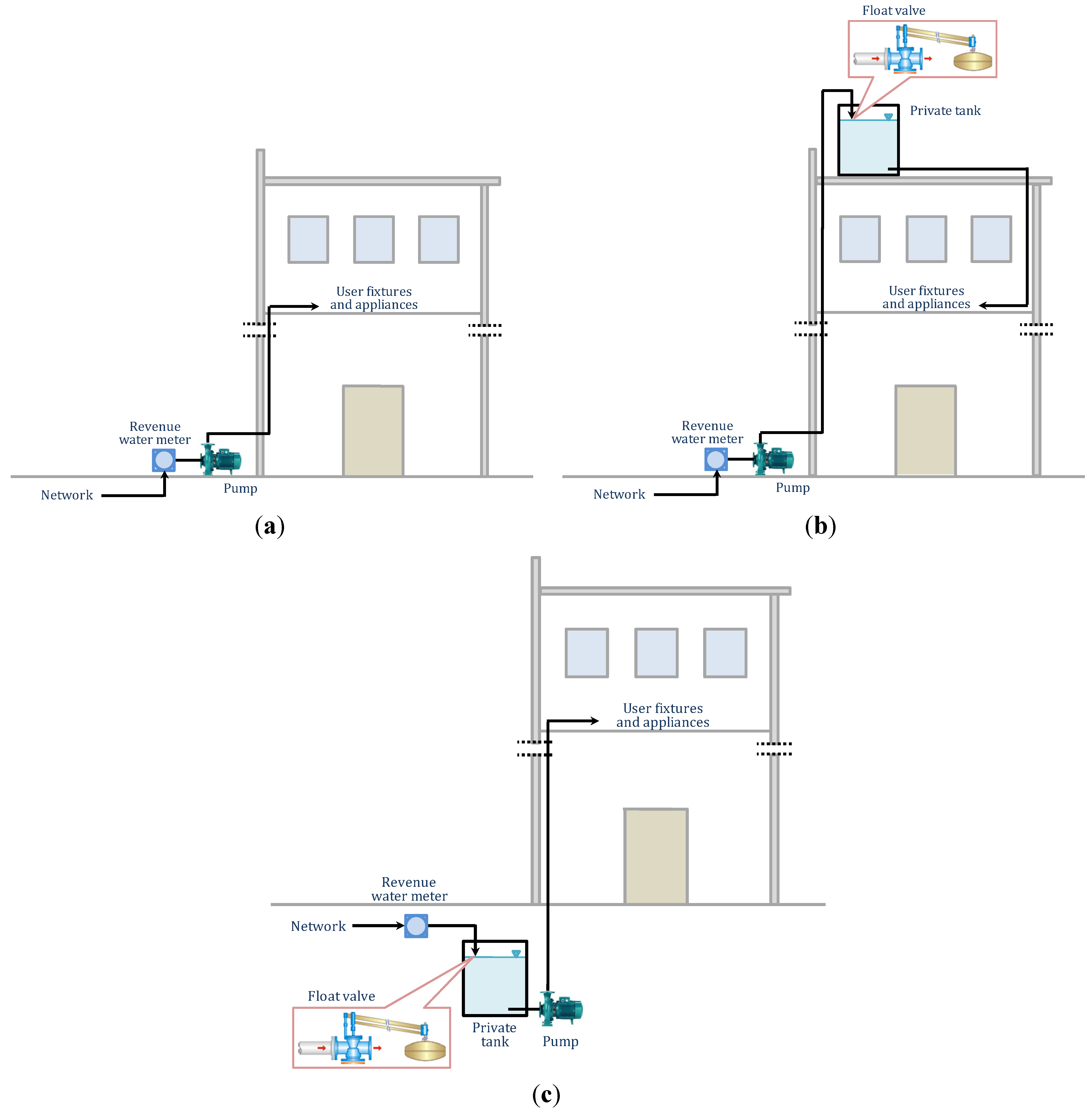
Energy impacts have been analysed in the literature by considering the effect of leakages [18,19]. The aim of this paper is to evaluate, at single node and network scale, the energy cost for users due to private tanks and pumping by analysing one of the supply networks of the city of Palermo (Italy). This analysis was carried out considering, first of all, a continuous supply service (Figure 1a), with users provided with private pumps only working when the pressure at the node is lower than the minimum required to have outflow, and then two discontinuous service configurations with users also provided with rooftop tank (Figure 1b) and underground tank (Figure 1c). In the rooftop tank scheme, the tank is fed by the pump directly connected to the network and users take water from the tank (Figure 1b). The pumping system works to fill the tank when the pressure on the network is too low to have outflow. In the underground tank scheme, the tank is filled by gravity and users have access to water by the pump installed downstream of the tank (Figure 1c).

To better understand and show the results of the analysis, some performance indicators dealing with pumping utilisation and energy consumption were taken into account.

2. The Proposed Methodology

In a water distribution system managed via intermittent supply, the cyclical filling and emptying processes occurring in the network modify the design operational conditions of the system. A reliable analysis of such operational conditions needed a dynamic mathematical modelling of the network. To this aim the authors developed a dynamic model for simulating the filling process of water distribution network managed via intermittent supply and where users acquired private tanks in order to reduce their vulnerability to service intermittency [6,7]. The model was applied to the same real case study described below. The analysis demonstrated that private tanks greatly affect the hydraulic behaviour of the network modifying the demand pattern of users. Users’ demand is much higher than normal at the beginning of the service period (during the network filling process) reducing the pressure level on the network and presenting some disadvantaged users to receive water supply. As result, the intermittent distribution generates high competition among users: those located in advantaged positions (near the network inlet node and/or at low height) are able to obtain water soon after the service period begins, while others have to wait much longer, after the network is full.

Although the dynamic modelling of the network would be more reliable, it is quite time and computational expensive. However, a steady-state model was adopted because the duration of the filling process of the network chosen as case study is quite short (about one hour) and because the main focus of this paper is the estimate of the users’ energy cost due to private tanks.

Figure 1. A schematic of the typical plumbing connection to: (a) the network provided with pump; (b) the rooftop tank; (c) the underground tank.

Figure 1. A schematic of the typical plumbing connection to: (a) the network provided with pump; (b) the rooftop tank; (c) the underground tank.

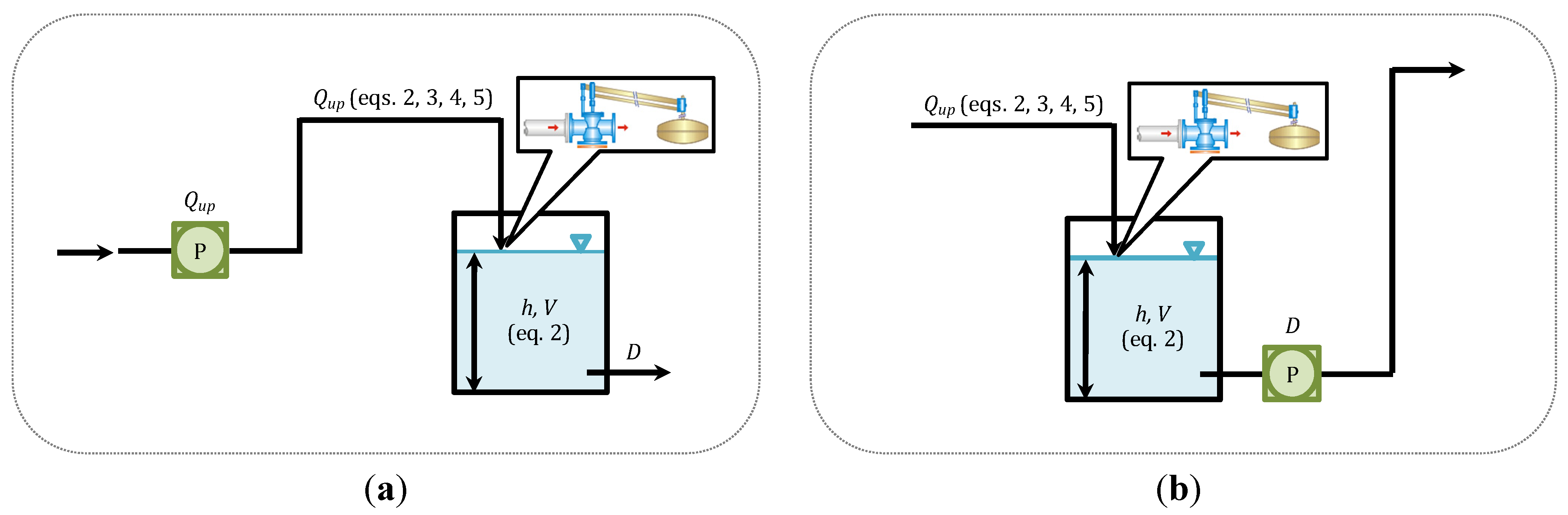
To analyse the users’ energy cost of intermittent distribution, some additions were implemented in EPANET [20] to take into account the pumping stations, the tank filling process and the variation of the tank inflow depending on the network pressure, on the float valve characteristics and on the tank water level and not on user demand. Figure 2 shows a schematic of the modelled elements with the indication of the main variables.

Figure 2. A schematic of the modelled pump-private tank system: (a) rooftop tank and (b) underground tank.

Figure 2. A schematic of the modelled pump-private tank system: (a) rooftop tank and (b) underground tank.

Apart of the plumbing connection scheme considered, the private tank filling and the user water resource accessibility greatly depend on the network pressure. In traditional demand-driven analysis, the network modelling is carried out by assigning the specific water demands of all the nodes and computing the nodal pressure heads and link flows from the equations of mass balance and pipe friction head loss [21]. In real networks, this simple, widely adopted approach can yield nodal pressures that are lower than the minimum required service level or even negative: in this condition design demands would not be met. 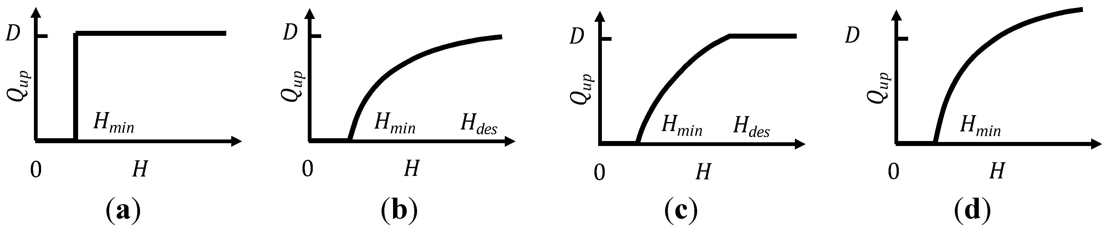Although this is a well-known problem and it has been tackled by many researchers [11,16,22,23,24,25,26,27,28,29], it is still sometimes ignored. Since the 1980s, various methods, generally termed head-driven analysis, have been proposed to compute actual water consumptions, network node pressures and flows involving an assumption on the relationship between pressure and outflow at the demand nodes (Figure 3). Furthermore, some questions are still open, especially on the definition of the law between supplied water volumes and network pressure.

Figure 3. Head-driven analysis methods: (a) Bhave [14]; (b) Germanopoulos [15]; (c) Wagner et al. [16]; and (d) Reddy and Elango [17]. $D$ = required outflow at network mode; $Q_{up}$ = available outflow at network mode; $H$ = available pressure at network mode; $H_{des}$ = desirable pressure at network mode to have $D$; $H_{min}$ = minimum pressure to have outflow at network mode.

Figure 3. Head-driven analysis methods: (a) Bhave [14]; (b) Germanopoulos [15]; (c) Wagner et al. [16]; and (d) Reddy and Elango [17]. $D$ = required outflow at network mode; $Q_{up}$ = available outflow at network mode; $H$ = available pressure at network mode; $H_{des}$ = desirable pressure at network mode to have $D$; $H_{min}$ = minimum pressure to have outflow at network mode.

As Figure 3d shows, the method introduced by Reddy and Elango [25] is completely different than the others: the pressure-consumption function does not have an upper boundary, and the node outflow is the maximum taken by the network, only related to the available nodal pressure $H$ according to the following equation:

$$Q_{up}=k\times {(H-H_{min})}^p$$

(1)

where $Q_{up}$ is the actual or available node outflow (upstream of the tank for the plumbing schemes in Figure 1b,c), $H$ is the node pressure, $H_{min}$ is the minimum pressure required to have outflow at the node, and $k$ and $p$ are calibration coefficients. With regard to the continuous distribution scheme (Figure 1a), $H_{min}$ can be fixed equal to the height of the user fixtures and appliances. In the present study it was fixed equal to the height of the barycentre of the buildings fed by the network node. With regard to intermittent schemes (Figure 1b,c), $H_{min}$ is equal to the average height of the buildings connected to the node if the tank is considered on the rooftop, or it is equal to zero if it is considered put underground.

Where the water distribution is periodically provided on intermittent basis, the users often modify their internal plumbing system with private tanks and pumps to collect as much water as possible even if nodal pressure is lower than the minimum required for outflow at the node. In such situations, the method proposed by Reddy and Elango [25] must be modified to take into account the presence of local tanks and floating valves that progressively reduce inflow volume while the tank is filling as well.

The addition to the EPANET model is based on the combination of the tank continuity equation [(Equation (2)] and the float valve emitter law [(Equation (3)]. The main model equations may be summarised as the following:

$$Q_{up}-D=\frac{dV}{dt}=A\times \frac{dh}{dt}$$

(2)

$$Q_{up}=C_v\times a\times \sqrt{2g\left(H-H_r\right)}$$

(3)

where $D$ and $Q_{up}$ are the user water demand and the discharge from the distribution network to the local tank, respectively; $V$ is the volume of the private tank with an area $A$ and variable water depth $h$; $C_v$ is the float valve emitter coefficient; $a$ is the valve effective discharge area; $H$ is the node pressure; $H_r$ is the height of the floating valve supplying the tank; and $g$ is the acceleration of gravity. The float valve emitter coefficient $C_v$ and the effective discharge area $a$ depend on the floater position and thus on water level of the tank according to the following empirical laws:

$$C_v=\{\begin{array}{c}if h<h_{min} \Rightarrow C_v=C_v^{*}\\ if h>h_{min}\Rightarrow C_v=C_v^{*}\times {\left(\frac{h_{max}-h}{h_{max}-h_{min}}\right)}^n\end{array}$$

(4)

$$a=\{\begin{array}{c}if h<h_{min} \Rightarrow a=a^{*}\\ if h>h_{min}\Rightarrow a=a^{*}\times {\left(\frac{h_{max}-h}{h_{max}-h_{min}}\right)}^m\end{array}$$

(5)

where $h_{min}$ and $h_{max}$ are the water depths at which the valve is fully open and fully closed, respectively; $C_v^{*}$ and $a^{*}$ are the emitter coefficient and the effective discharge area of the fully open valve, respectively; and $n$ and $m$ are shape coefficients, usually ranging between 0.5 and 2.0, that must be experimentally estimated. The energy required for pumping can be then integrated in the model with the common formula:

$$E={\int }_T\frac{1}{\eta }·\gamma ·Q·H·dt$$

(6)

where $T$ is the pump working time; $\eta$ is the pump output coefficient; and $\gamma$ is water specific weight. $Q$ is the pumped flow and it is equal to $Q_{up}$ when the pump is directly connected to the network and no private tank is put between the network and the user (continuous distribution scenario) and when the private tank is on the rooftop; it is equal to $D$ when the tank is put underground. $\text{Δ}H$ is $H_{min}-H$ if the tank is put on the rooftop and $H_{min}>H$ , and it is equal to the average user height if the tank is underground.

The add-on model parameters were set equal to the average obtained in a field campaign that has been carried out in the same network since 2007 [11]. Several users with tanks have been monitored to investigate apparent losses due to water meter under-registration. Data were collected to calibrate the add-on model. Details are provided in [11,29]. $C_v^{*}$ was set equal to 0.57, $a^{*}$ was set to 2.8 cm², and $m$ and $n$ were set equal to 0.85 and 0.78, respectively. The pump output coefficient $\eta$ was fixed equal to 0.72 in the present study according with the average value of the type of pumps adopted for this use.

3. The Case Study

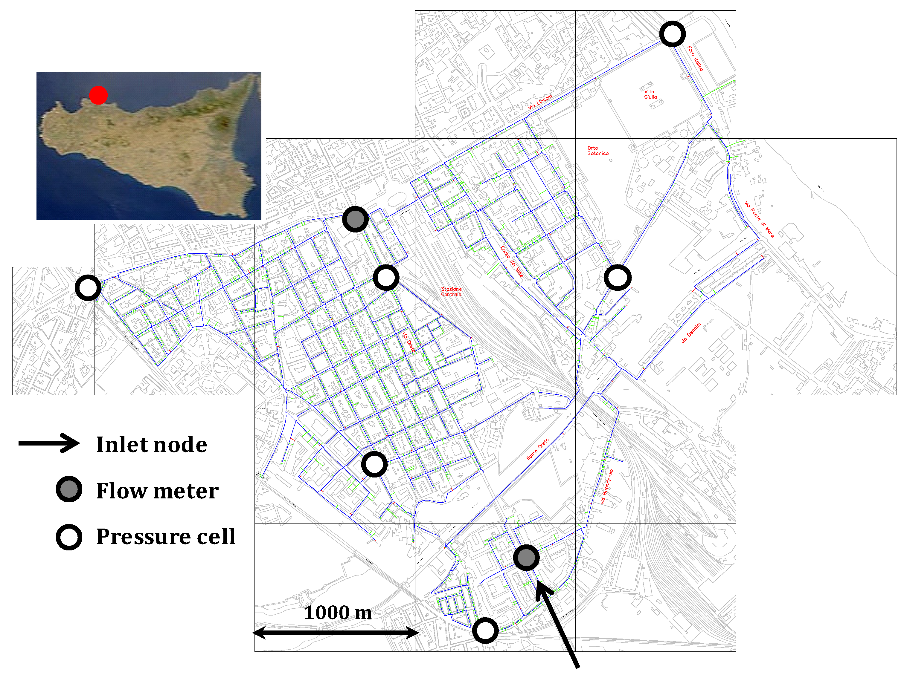
The model was applied to one of seventeen supply networks in the city of Palermo (Italy). Figure 4 shows a schematic of the network adopted in the study.

Figure 4. A schematic of the network.

Figure 4. A schematic of the network.

This network was chosen because it was recently rebuilt, and all its geometric characteristics, the number and the distribution of user connections, the water volumes delivered and measured, and the pressure and flow values in a few important nodes are precisely known. The renovation process took place in the sole distribution network, keeping in service the old cast-iron feeding pipes. 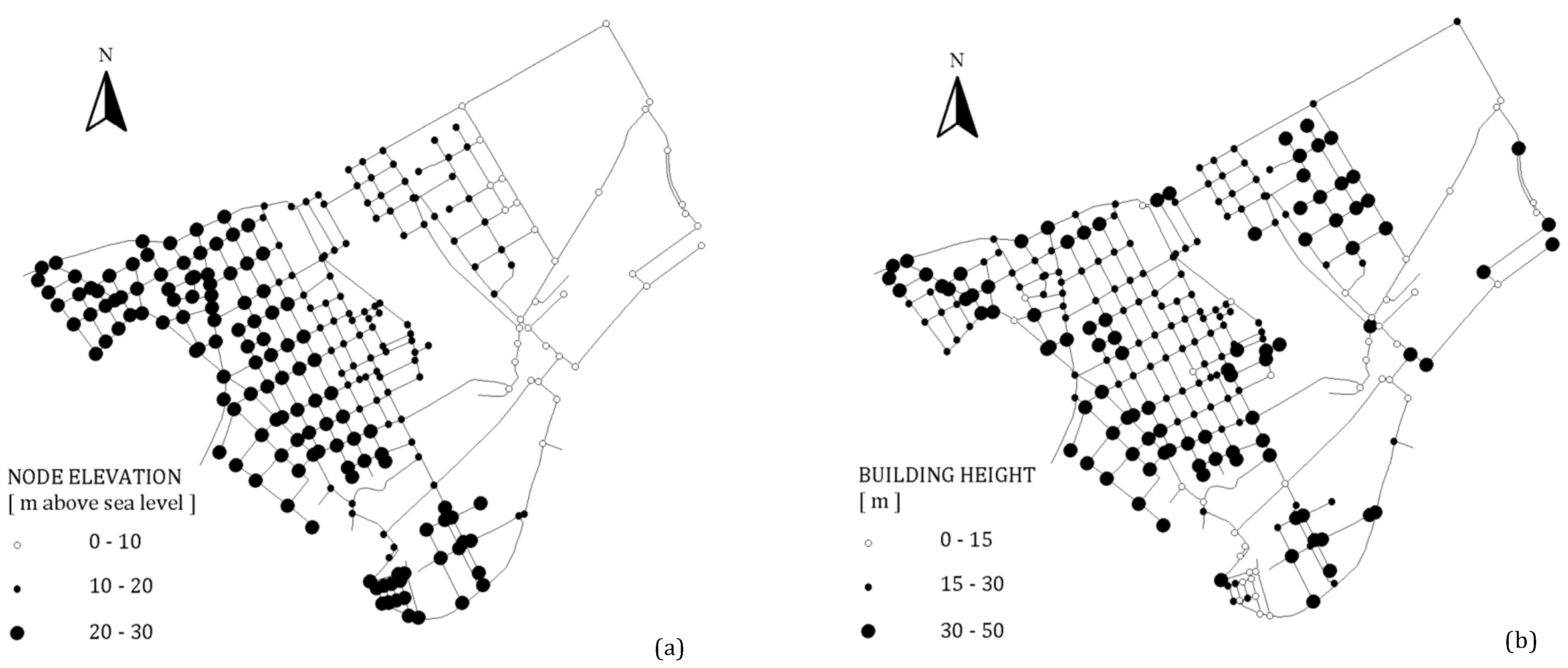The network is fed by two reservoirs at different levels that can store up to 40,000 m³ per day and supply nearly 35,000 inhabitants (8700 user connections). The network is about 40 km long, and the pipes are made of polyethylene, with diameters ranging between 110 mm and 225 mm. Network node (street level user connections) elevation ranges between 3 m and 47 m above sea level (Figure 5a), while building height ranges between 5 m and 50 m (Figure 5b).

Figure 5. (a) A map of the network node elevation; (b) A map of the corresponding average building height.

Figure 5. (a) A map of the network node elevation; (b) A map of the corresponding average building height.

The network was designed to deliver about 400 L/capita/day, but the actual average consumption is about 260 L/capita/day. As consequence, under ordinary conditions, the network is characterized by low water velocities and correspondently high pressures, which resulted in substantial leakage in the past. These conditions, together with the recurrent lack of water resources, did not permit continuous distribution over the last five years (at least during the summer period); intermittent distribution on a daily basis was introduced as a common practice, leading users to acquire local private tanks. Furthermore, because of the significant water loss that occurs in the feeding pipe that connects the reservoirs with the network, the water utility decided to reduce the pressure level on the network. This further encouraged users to maintain their own storage tanks to prevent temporary interruptions in water supply and to adopt a local pumping system to feed the tanks if the network pressure is not adequate. Typically, the private tanks have specific volumes equal to 200–250 L/capita; this assumption was adopted for this analysis.

The system is monitored by six pressure cells and two electromagnetic flow meters (Figure 4). Data have been provided on hourly basis almost continuously since 2001, and the network hydraulic model calibration is constantly updated when new data become available [16,17].

4. Results and Discussion

The network was analysed considering three configurations of user plumbing scheme connection at the network node: a continuous distribution and two intermittent distribution configurations, respectively, with all users fed by private pumps and roof tanks or by underground tanks and pumps. In the first configuration (continuous distribution), users do not have private tanks but rather pumping systems that only work when the pressure is lower than the minimum required to feed them. The three selected configurations were analysed as limit cases in order to evaluate the range of potential energy consumption and the related cost met by users due to private pumps and tanks to supply. The actual energy consumption depends on the actual presence of these plumbing connection schemes.

The construction and invoice costs of equipment needed for the installation of the private pump-tank set and the maintenance costs should be considered in the present study together with the user’s energy consumption costs. The annual invoice or construction costs linked to private tanks are negligible due to the low cost and the long service life of the tank. Furthermore, the underground tanks are usually built together with the buildings. In the same way, the annual maintenance costs related to the cleaning and disinfection of the private tank together with the “coping costs” with the disinfection of the water volume staying in the private tank can be neglected. Frequently, above all in the southern Italy, users prefer to not drink tap water because they do not have confidence of the reliability of the water supply system. The main part of the cost of private pump-tank set is due to the invoice and maintenance of the pumping system present in each of the three configurations considered. Even if the pumping power required is different, the invoice and maintenance costs of the pump can be considered similar. For this reason these costs were not accounted for in the present analysis.

To better understand and show the analysis results, some performance indicators dealing only with pumping utilisation and energy consumption and cost were taken into account [30]: the ratio between the daily energy and water consumption (PI1), the ratio between the daily energy and water cost per cubic meter delivered to the users (PI2), the ratio between the daily energy cost and water consumption (PI3) and the daily energy consumption per capita (PI4). The energy cost was fixed equal to 0.22 Euro/kWh and the water cost equal to 1.10 Euro/m³.

In continuous distribution, the energy consumed by the private pumping system and thus the relative cost met by users were close to zero. When the service is continuous, the pumping system supplies only the building apartments over the network pressure level, so the volume delivered and the power required are very small. Therefore, this first condition was neglected in the analysis carried out on the network node basis.

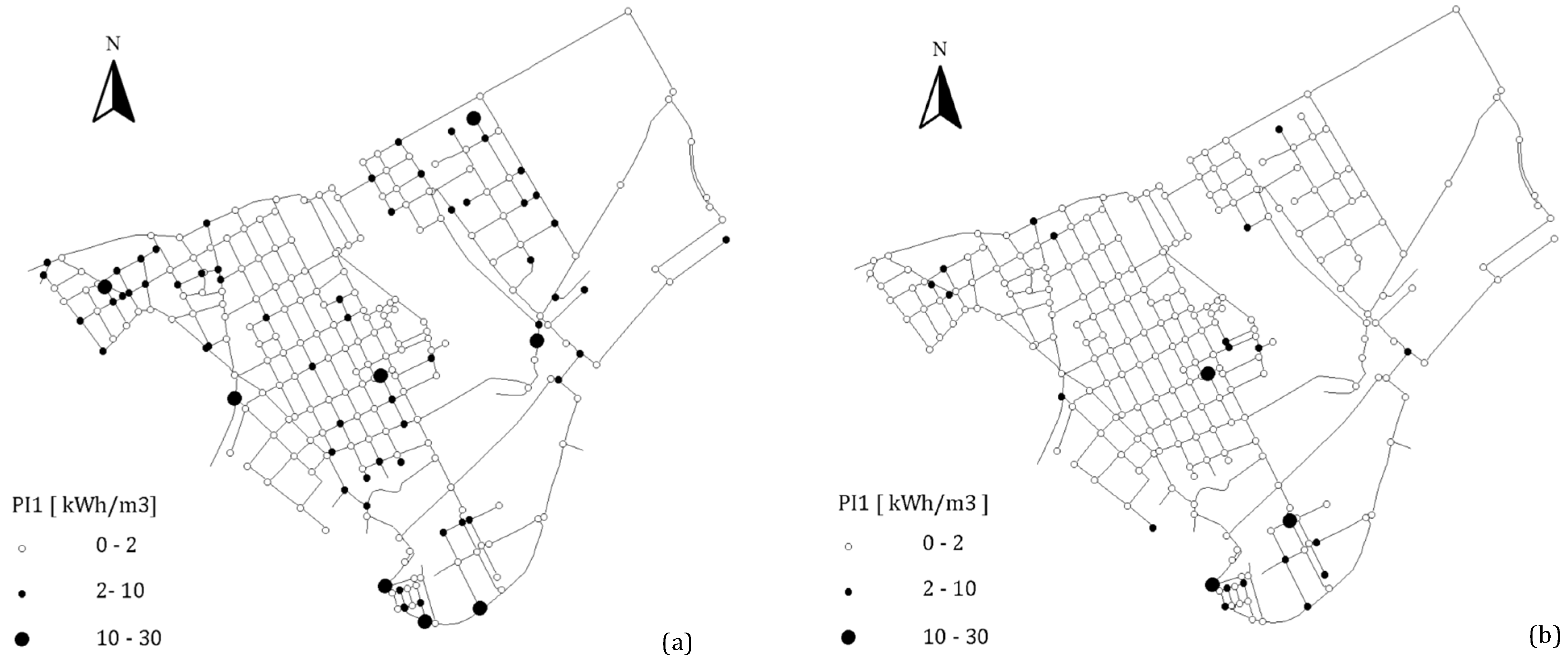
Figure 6 and Figure 7 show the PI1 and PI2 values at each node of the network operating in the other two configurations taken into account. The distribution of PI values shows a complex situation in which some users are characterised by a very large energy costs depending on the characteristics of the buildings and the network pressures.

In intermittent distribution with underground tanks, as discussed above, the tank is fed by the network by gravity, and the users are supplied by a private pumping station installed downstream of the tank. Then, the pumping system supplies the entire building with the entire user demands without any dependence on the network pressure. In intermittent distribution with roof tanks, the pumping system only works when the pressure is lower than the minimum required to feed the tank. The power required has to cope only with the difference between the network water head and the building rooftop elevation. The pump is then turned off if the tank is full or the water head is sufficient for supplying the tank by gravity.

Figure 6. PI1 node values: (a) intermittent distribution with underground tank and (b) intermittent distribution with rooftop tank.

Figure 6. PI1 node values: (a) intermittent distribution with underground tank and (b) intermittent distribution with rooftop tank.

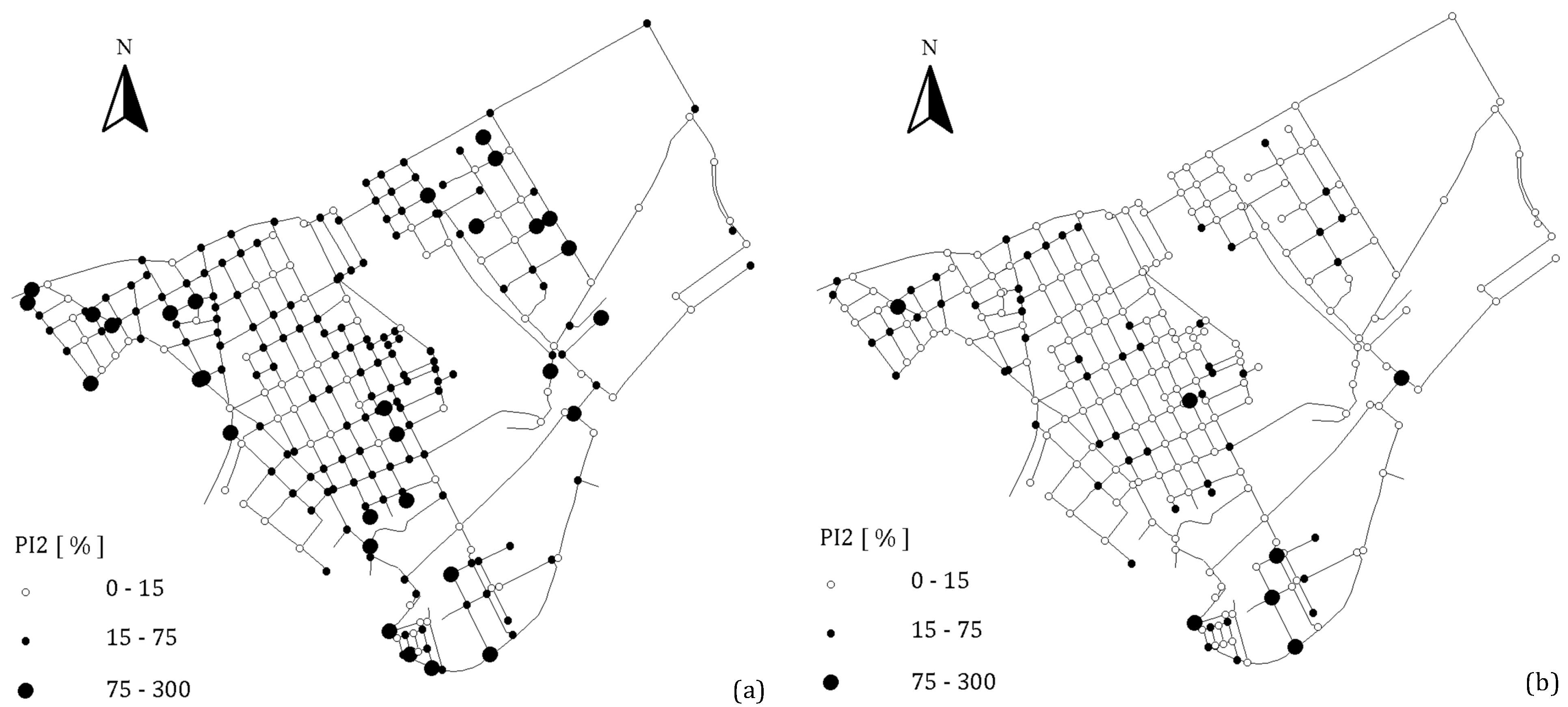
Figure 7. PI2 node values: (a) intermittent distribution with underground tank and (b) intermittent distribution with rooftop tank.

Figure 7. PI2 node values: (a) intermittent distribution with underground tank and (b) intermittent distribution with rooftop tank.

Therefore, in the two tank schemes, the pumping stations act on different water volumes requiring different energy consumption. Aggregating the results at the network node scale, the underground tank scheme generates energy consumptions greater than the roof tank scheme (Figure 6 and Figure 7). However, in a few nodes the roof tank- pumping system installation caused greater energy consumption because of the difference between the building roof top elevation and the network water head. Thus, the building height is the key factor to assess the energy consumption. In the underground tank scheme, the energy consumption is directly related to the height of the building supplied by the pumping system installed downstream of the tank. In the roof tank scheme, only when the pumping system is working because network pressure is too low to feed the tank by gravity does the energy consumption depend on the difference between the network water head and the building height. Otherwise, the energy consumption is zero. Therefore, it is not possible to establish the most energy expensive scheme: it depends on the difference between the building height and the network water head. When this difference is about the same as the building height, the underground tank scheme causes lower energy consumption; otherwise, the roof tank scheme is the least expensive installation.

As Figure 6a shows, the energy consumption per m³ of water resources drawn from the underground tank is 0–2 kWh for 77% of users, 2–10 kWh for 20% of users and 10–70 kWh for 3%. The same considerations may be applied for the roof tank scheme: Figure 6b shows the percentages of users that have to utilise 0–2, 2–10 and 10–30 kWh for drawing 1 m³ from the public network to feed the roof tank are 90%, 9% and 1%, respectively. The corresponding energy cost can be evaluated by the mean of PI2. Figure 7a shows that the energy cost represents 0%–15% of the water cost per cubic meter consumed by the users for 30% of users, 15%–75% for 60% of users and 300% for 10% of users. Figure 7b shows that the 70% of users have to pay an energy cost in the range between 0% and 15% of the water cost; the 27% of users are subjected to energy costs comparable with the half of water costs (between 15% and 75% of the water costs); for 3% of the users, the cost of energy represents the most part of the amounts to have to pay for water supply (energy cost is between 75% and 300% of water cost). Even more interestingly, the cost of the supplied water cubic meter can be four times higher for the most disadvantaged users than the most advantaged ones. The results demonstrate that the inequalities that intermittent distribution can create in terms of access to water resources are intensified by the presence of additional energy costs that are paid only by some of the users inside the network depending on their positional disadvantage.

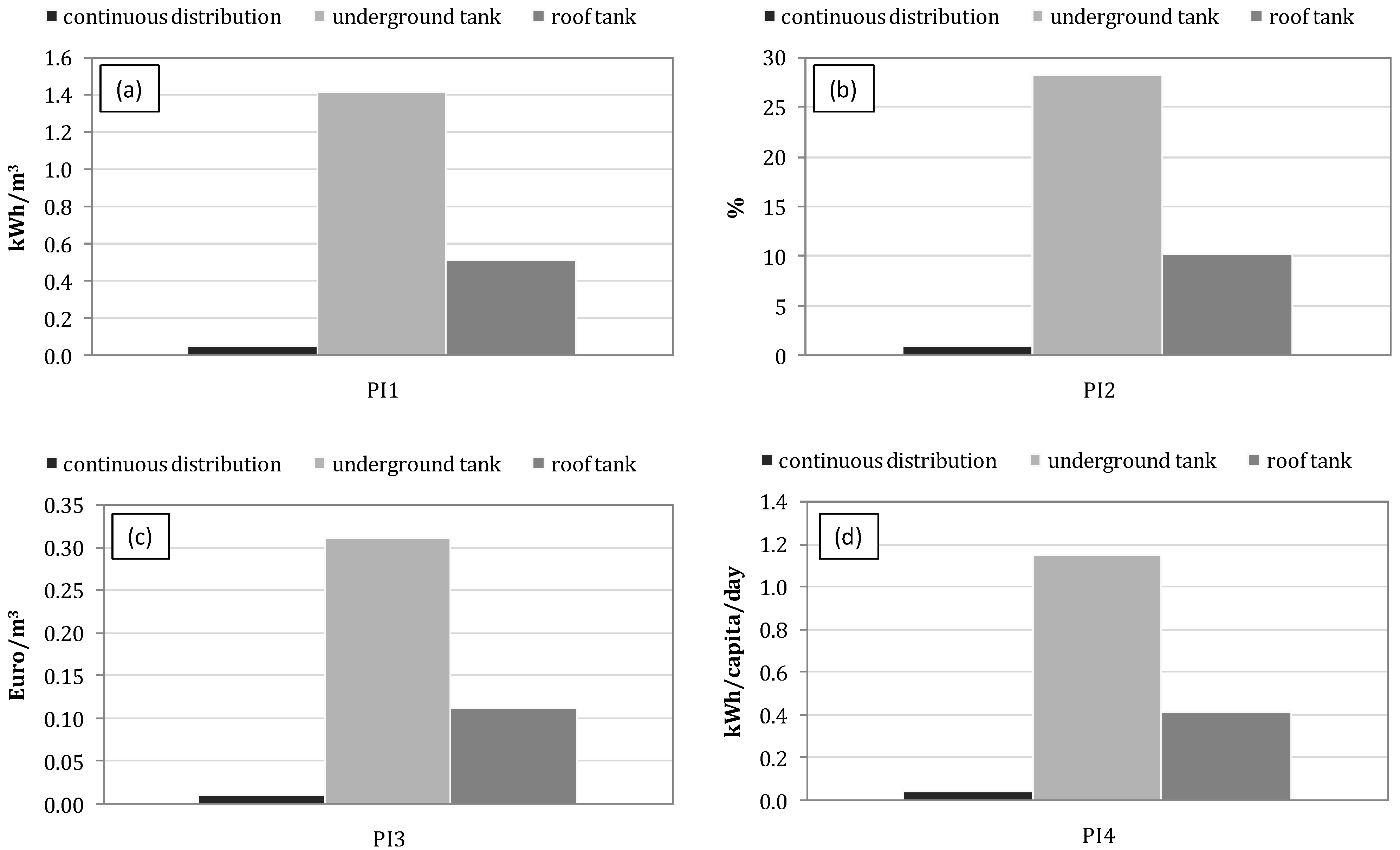
Considering the entire network, all the proposed indicators were assessed for the three configurations (Figure 8). In this way, a global evaluation of the energy impact was done.

Figure 8. Comparison between the PIs value assessed for the entire network in the three scenarios: (a) PI1, (b) PI2, (c) PI3 and (d) PI4.

Figure 8. Comparison between the PIs value assessed for the entire network in the three scenarios: (a) PI1, (b) PI2, (c) PI3 and (d) PI4.

The PIs have confirmed the intermittent condition with underground tanks was globally the most energy expensive. While in continuous distribution users do not spend energy and money to draw water resources from the network (the four indicators are close to zero), the underground tanks and the roof tanks have a daily energy consumption per m³ of about 1.4 kWh and 0.5 kWh, respectively. The corresponding average cost is about 0.3 Euros per m³ and about 0.12 Euros per m³. The ratio between daily energy and water cost (PI2) shows that the energy cost globally represents about 30% (underground tank scheme) and 10% (roof tank scheme) of the water cost per cubic meter delivered to the users. To summarize, Figure 8b shows that the average cost of water supply at the network scale is increased by 10% to 30%, depending on the local tank scheme adopted. This network average gives the dimension of the problem, but Figure 6 and Figure 7 show the high differences among users: service intermittency does not only provide inequalities in terms of access to water resources [6,16,17] but also different costs that have to be supported by users depending on their location. The average values, provided in Figure 8b, have to be compared with the geographically distributed analysis provided in Figure 7 that shows the maximum of energy cost that is in the range of 300% of the water cost per cubic meter delivered to the users.

4. Conclusions

This present paper reports the results of an analysis of the energy that users have to pay for drawing water resources from the public network because of private storage tanks and pumping systems. The research proposed a new node demand model to take into account the complexity of systems made up of underground tanks or roof tanks. The model was implemented in EPANET and applied to a real case study. The network chosen was analysed by considering, first of all, a continuous distribution, without private tanks and with pumps only working when the pressure is lower than the minimum required to feed users, then with all the users fed by the system with pumps and roof tanks and finally by the system with underground tanks and pumps. To better understand and show the analysis results, four performance indicators dealing with pumping utilisation and energy consumption were taken into account.

The results showed that private storage tanks have a relevant impact on user energy consumption. In continuous distribution, the energy consumed by the pumping system and thus the relative energy cost were close to zero. In intermittent distribution, the energy consumed depends on the tank scheme chosen. In the underground tank scheme, the energy consumption is directly related to the height of the building supplied by the pumping system installed downstream of the tank. In the roof tank scheme, only when the pumping system is working does the energy consumption depend on the difference between the network water head and the building height. The underground tank scheme involves energy consumptions greater than the roof tank scheme for most of the network. However, in a few nodes, the roof tank-pumping system installation causes greater energy consumption. In some nodes, the energy consumption per m³ reached a value of 30 kWh/m³, and the ratio between the corresponding energy cost and water cost per cubic meter delivered to the users showed a maximum value of 300%. Considering the entire network, the indicators confirmed that the underground tank scheme was the most energy expensive. This result depends on the different volumes involved in the two tank schemes: the pumping system installed downstream of the underground tank supplies the entire building with the whole user demand; with the roof tank, the pump only works when the network pressure is lower than the minimum required to feed the tank, and then only the volume that does not enter the tank by gravity is pumped.

While in continuous distribution, users do not spend energy and money to draw water resource to the network, the underground tanks and the roof tanks require a daily energy cost of about 0.3 Euro/m³ and about 0.15 Euro/m³, respectively. The ratio between the daily energy and water cost show that the energy cost represents about 30% (underground tank scheme) and 10% (rooftop tank scheme) of the water cost per cubic meter delivered to the users. The obtained results representing the range of the possible additional costs for users to supply water highlighted the problem connected to the intermittency of the water supply service.

The analysis showed that intermittent distribution causes inequalities not only in user access to water resources but also in costs that users have to support to have access to water. Advantaged users may not need the presence of a pumping system, and thus their additional costs are null; otherwise, disadvantaged users may require massive use of pumping systems, thus greatly increasing the overall cost of water service.