Modeling of the Partial Discharge Process in a Liquid Dielectric: Effect of Applied Voltage, Gap Distance, and Electrode Type

Abstract

The partial discharge (PD) process in liquid dielectrics is influenced by several factors. Although the PD current contains the information representing the discharge process during the PD event, it is difficult to determine the detailed dynamics of what is happening in the bulk of the liquid. In this paper, a microscopic model describing the dynamics of the charge carriers is implemented. The model consists of drift-diffusion equations of electrons, positive and negative ions coupled with Poisson’s equation. The stochastic feature of PD events is included in the equation. First the model is validated through comparison between the calculated PD current and experimental data. Then experiments are conducted to study the effects of the amplitude of the applied voltage, gap distance and electrode type on the PD process. The PD currents under each condition are recorded. Simulations based on the model have been conducted to analyze the dynamics of the PD events under each condition, and thus explain the mechanism of how these factors influence the PD events. The space charge generated in the PD process is revealed as the main reason affecting the microscopic process of the PD events.

1. Introduction

For many applications, liquid dielectrics are superior to solid or gaseous electrical insulation materials. Advantages of liquids include higher breakdown strength compared to compressed gases. When compared with solid dielectrics, their ability to circulate leads to better thermal management and easier removal of debris after breakdown or degradation. Liquid dielectrics are also better suited to applications involving complex geometries. Thus the electrical behavior of dielectric liquids subjected to high electric fields has been intensively studied [1]. The interest arises from various applications that include pulsed power systems, energy storage, highvoltage insulation, development of acoustic devices and spark erosion machines.

Partial discharge (PD) measurement and analysis in liquid dielectric has become an essential tool in on-line monitoring systems to evaluate the performance of insulation systems. Many researches have been undertaken focusing on related areas [2,3,4]. Partial discharge in dielectric liquids is a very complex process that involves a succession of inter-correlated phenomena (electronic, mechanical, thermal, etc.). Moreover, experiments have shown that characteristic features of partial discharge phenomena greatly depend on experimental conditions (electrode geometry, shape and amplitude of applied voltage, liquid nature and purity, etc.). However, as a result of their small amplitude and wide bandwidth, it is difficult to find the relationship between the measured PD current and the physical mechanisms that occur during the event itself. Consequently the modeling of PD is important in providing a better understanding of this phenomenon.

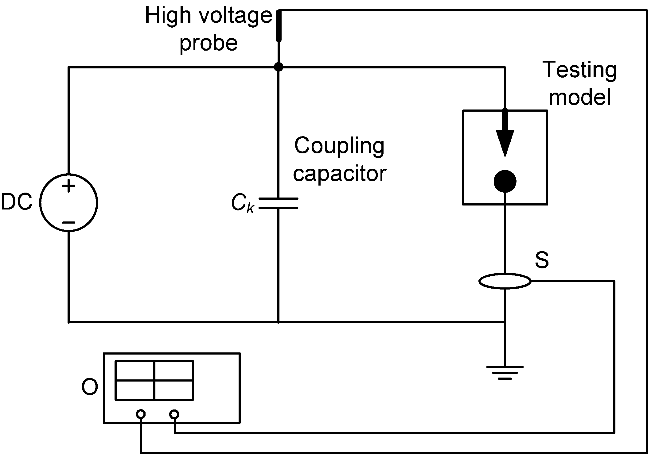
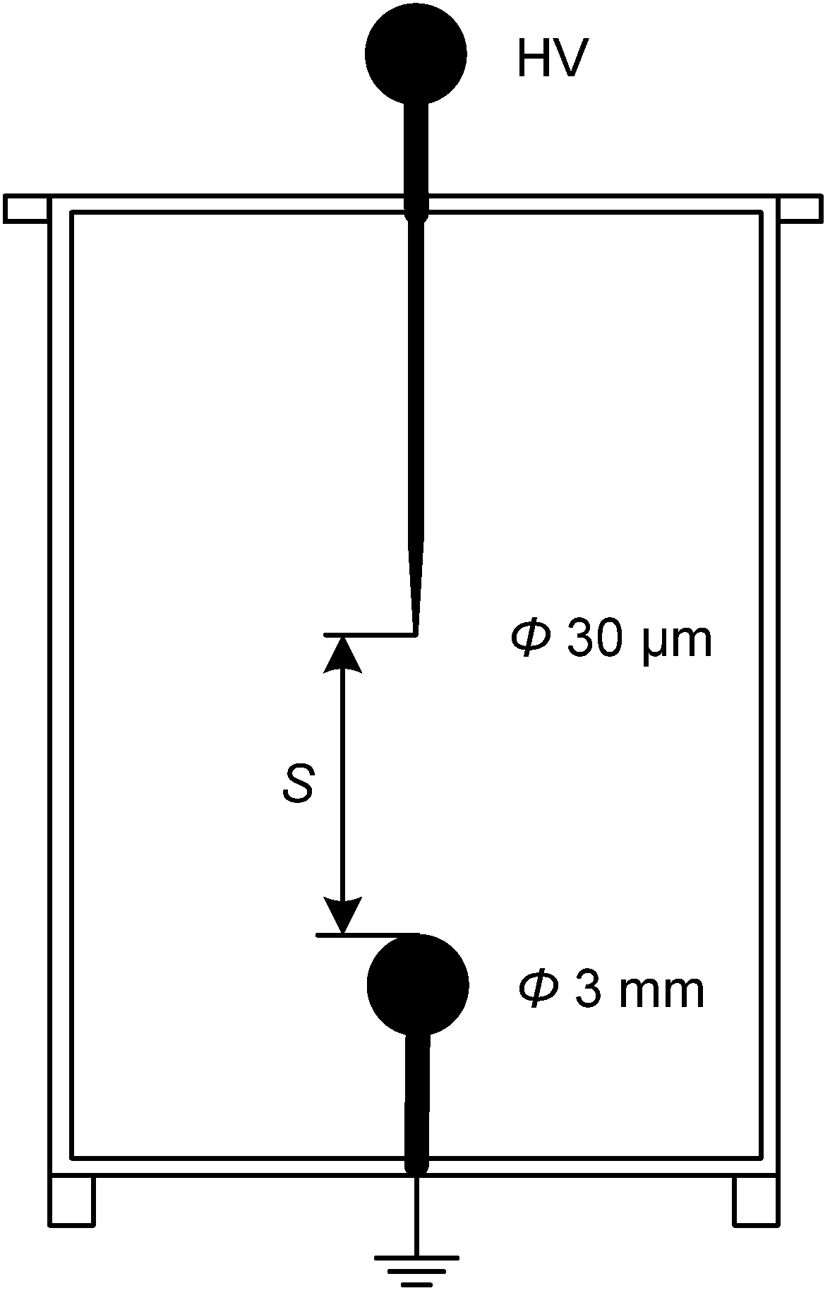
In previous research concerning gas discharge mechanisms, the implementation of the electro-hydrodynamic model has been validated in describing the discharge process [5,6]. Also, breakdown processes in transformer oil have been investigated based on a similar physical and mathematical theorem [7,8]. By treating liquid dielectrics as a dense fluid, the drift-diffusion equations of positive ions, negative ions and electrons are solved coupled with Poisson’s equation in this work. Rather than attempt to treat all phenomena associated with breakdown, it has been decided for the sake of clarity and brevity to restrict discussion in this paper to DC partial discharge process occurring in mineral transformer oil. The finite element method based commercial software Comsol Multiphysics is used for numerical calculations. A 2D axisymmetric needle-sphere electrode configuration is utilized. The PD process simulation is modeled as a response to a positive DC voltage applied to the needle electrode. First the model is validated through comparison of the PD current between simulation and experimental results. Then the effect of amplitude of applied voltage, gap distance, electrode type on the PD process is analyzed based on estimations of the main features of the PD process.

2. Experimental Setup

Figure 1 shows a schematic diagram of the experiment setup used in this work to measure PD activity. The experiment consists of high voltage direct current voltage supply (maximum 50 kV). A coupling capacitor Ck with 2000 pF is used as circuit of the PD current. The PD current is coupled by a Rogowski coil sensor with bandwidth of 40 MHz. A digital oscilloscope is used to observe and record PD signals. The sampling frequency of the oscilloscope for recording PD signals is 1 GS/s.

Figure 1. Schematic diagram of the partial discharge experimental setup.

Figure 1. Schematic diagram of the partial discharge experimental setup.

Figure 2 shows a schematic diagram of the test sample used both in experimental and simulation studies. In order to obtain a reliable PD generation from the stressed electrode, a needle-sphere electrode configuration is utilized. The electrode configuration of the sample consists of a stressed needle electrode with tip radius of 15 μm and an earthed sphere electrode with radius of 1.5 mm, separated by a gap distance S. Two gap distance values are utilized which are 5 mm and 10 mm, respectively. The test sample is immersed in transformer oil.

Figure 2. Schematic diagram of the experimental test sample.

Figure 2. Schematic diagram of the experimental test sample.

3. Model Description

With the treatment of liquid dielectrics as a dense fluid, the hydrodynamic drift-diffusion model consisting of three charge carriers is utilized accounting for the movement, generation and loss of electrons, positive and negative ions and for the development of space charge. The continuum equations of the charge carriers are coupled with Poisson’s equation and consequently the effect of space charge on the electric field is included. The equations are given as:

$$\frac{\partial N_p}{\partial t}=G\left(\left|\mathit{E}\right|\right)F-N_e{N}_p{\beta }_{ep}-N_n{N}_p{\beta }_{np}-\nabla \bullet \left(N_p{\mathit{W}}_{\mathit{p}}\right)$$

(1)

$$\frac{\partial N_e}{\partial t}=G\left(\left|\mathit{E}\right|\right)F-N_e{N}_p{\beta }_{ep}-\nabla \bullet \left(N_e{\mathit{W}}_{\mathit{e}}\right)$$

(2)

$$\frac{\partial N_n}{\partial t}=-N_n{N}_p{\beta }_{np}-\nabla \bullet \left(N_n{\mathit{W}}_{\mathit{n}}\right)$$

(3)

$$\nabla \bullet \left({\epsilon }_r\nabla V\right)+\frac{e}{{\epsilon }_0}\left(N_p-N_e-N_n\right)=0$$

(4)

where t is time, e the electronic charge, ε₀ the vacuum permittivity and ε_r the relative permittivity of the medium, V the electric potential; N_e, N_p and N_n the electron, positive and negative ion concentrations, respectively; W_e, W_p and W_n the electron, positive and negative ion drift velocities; $G\left(\left|\mathit{E}\right|\right)$, and β, the ionization, and recombination coefficients for electrons and positive and negative ions, respectively. The swarm parameters are given in Table 1 [7,8].

Table 1. Swarm parameters.

Parameters	Expressions
We	10−4E
Wp	10−9E
Wn	10−9E
βnp	1.64×10−17 m3s−1
$a$	3×10−10 m
m*	9.1×10−32 kg
n0	1023 m−3
∆	7.1 eV

Table 1. Swarm parameters.

Parameters	Expressions
We	10−4E
Wp	10−9E
Wn	10−9E
βnp	1.64×10−17 m3s−1
$a$	3×10−10 m
m*	9.1×10−32 kg
n0	1023 m−3
∆	7.1 eV

The generation term $G\left(\left|\mathit{E}\right|\right)F$ of charge carriers consists of two parts, which are respectively the generation rate $G\left(\left|\mathit{E}\right|\right)$ and a stochastic term represented by F. The generation rate $G\left(\left|\mathit{E}\right|\right)$ is modeled based on Zener tunneling model [9]:

$$G\left(\left|\mathit{E}\right|\right)=\frac{e^2{n}_{0}a\left|\mathit{E}\right|}{h}\text{exp}\left(-\frac{{\pi }^2{m}^{*}a{\mathrm{∆}}^2}{e{h}^2\left|\mathit{E}\right|}\right)$$

(5)

where e is the electronic charge, $a$ is the molecular separation, E is the electric field, h is Planck’s constant, m^* is the effective electron mass in the liquid, n₀ is the number density of ionisable species and ∆ is the molecular ionization energy.

In the real situation the transformer oil cannot be treated as ideal dielectrics with homogeneous bulk characteristics. The impurities, bubbles, and variation of dielectric constant may lead to fluctuation in the local micro-fields acting on the molecules. Meanwhile the micro dynamics of charge carriers including the collision process of the electrons into the oil molecules is also characterized with stochastic features. In former research [10,11,12,13,14,15] it has been shown that the probability of the discharge events in local area of dielectrics should depend upon magnitude of local electric field strength in this area. In some macroscopic models developed from the L. Niemeyer, L. Pietronero, H.J. Wiesmann (NPW) method and lattice gas automata algorithm, a power-law dependant function with respected to the electric field strength is implemented as the probability density function [16,17,18]. In this model, the probability density of the generation term can be expressed with similar function. With the generation rate calculated with Equation (5), it is unnecessary to set any cut-off voltage as the criteria for the stop of the discharge event. Compared with the implementation of cut-off voltage as criteria, which is generally dependant on the empirical expression and may lead to a stepwise change of the discharge process, the product of the generation rate and the stochastic term, which are both based on the electric field strength, will continuously decrease with the weakening electric field until the electric field strength is not high enough to sustain generation of charge carriers.

The P = A($\left|\mathit{E}\right|$/E_b)ⁿ is chosen as the probability density function in this model, where A, E_b, and n are respectively non-dimensional constant, threshold electric field strength, and power index [10,11,12,13,14,15]. These parameters are greatly dependant on the experimental conditions. Generally A is a non-dimensional constant with the value less than 10. The threshold electric field strength for the transformer oil discharge is around 10⁸–10⁹ V/m [7,8]. Also, in some literatures describing the oil discharge inherited from NPW method, the choice of power index n varies from 1 to 4. Based on our former research, the specific values for A, E_b, and n corresponding to this experimental condition can be respectively chosen to be 1 for A, 10⁹ for E_b, and 4 for n.

With the definition of probability density function, the incremental probability W, that there will be the generation of charge carriers during time t to t + τ, can be expressed as:

$$\text{d}W=\left(1-W\right)P\text{d}t$$

(6)

The solution to this equation can be expressed as:

$$W=1-\text{exp}\left(-P\tau \right)$$

(7)

However, the probability for the charge carrier generation is a calculated number between 0 and 1. In order to make it a random process, the stochastic term F is introduced:

$$F=H\left(W,r\right)$$

(8)

where H represents the Heaviside function and has a stepwise jump from 0 to 1 when W becomes larger than r. r is a random number, which evenly distributes on the range of (0,1), generated at every calculation node and time. Thus the product of generation rate $G\left(\left|\mathit{E}\right|\right)$ and the stochastic term F can describe the stochastic generation process of charge carriers.

The discharge current of the external circuit is calculated based on Sato’s equation [19]. By integrating the charged particle fluxes through the cathode surface plus the changes of the induced surface charge at the cathode, the current can be expressed as:

$${\mathit{I}}_S={{\displaystyle \oint }}_{\text{cathode}}\left[\left({\mathit{J}}_{\mathit{e}}+{\mathit{J}}_{\mathit{n}}+{\mathit{J}}_{\mathit{p}}\right)\bullet \mathit{n}\bullet \text{d}\mathit{S}+\frac{\text{d}}{\text{d}t}\left({\mathit{E}}_{\text{cathode}}\bullet \text{d}\mathit{S}\right)\right]$$

(9)

Multiplying the discharge current with the transform function of the current sensor generates the simulated PD waveform.

For Poisson’s equation, the boundary condition of the needle electrode is set as stressed electrode, and the sphere electrode is earthed according to the experimental setup. The outer insulating boundaries have been set to have zero normal displacement field components. For the drift-diffusion equations, the outer boundaries are set to have no flux of any charge carriers. Considering the repetitive rate is small for a DC partial discharge process, the simulation work is restricted to a single pulse process. Thus the electrode boundary condition for the charge drift-diffusion equations is convective fluxes for all species.

4. Validation of the Model

The partial discharge current essentially contains all the information of the partial discharge process. Thus the comparison between the PD current of the simulation result and the experiment data can represent the accuracy of the model. Before simulation, the permittivity of the transformer oil should be chosen. However the permittivity of mineral transformer oil can vary in a certain range according to its specific composition. Even using the same source of oil, the permittivity also can be different from its initial condition as a result of the storage and testing environment. The permittivity will affect the electric field distribution and consequently parameters related to electric field strength. In order to obtain an accurate simulation result, five different relative permittivity values based on physical characteristics of mineral transformer oil (2.0, 2.1, 2.2, 2.3 and 2.4) are chosen. The PD currents as a response to 1.2 and 1.5 partial discharge inception voltage (PDIV) under 5 mm and 10 mm gap distance are calculated. As the model is characterized with stochastic characteristics, the simulation is conducted 10 times for each experimental condition and the mean value of the 10 PD currents are compared with the measured value of the same experimental condition. The mean square error e between the simulation and the measurement result is calculated as follows:

$$e=\frac{{{\displaystyle \sum }}_{i=1}^N{[\frac{x_{\text{simulation}}\left(i\right)-x_{\text{measurement}}\left(i\right)}{x_{\text{measurement}}\left(i\right)}]}^2}{N}$$

(10)

where i represents the sampling point decided by the sampling frequency of the experiment and N equals 1000.

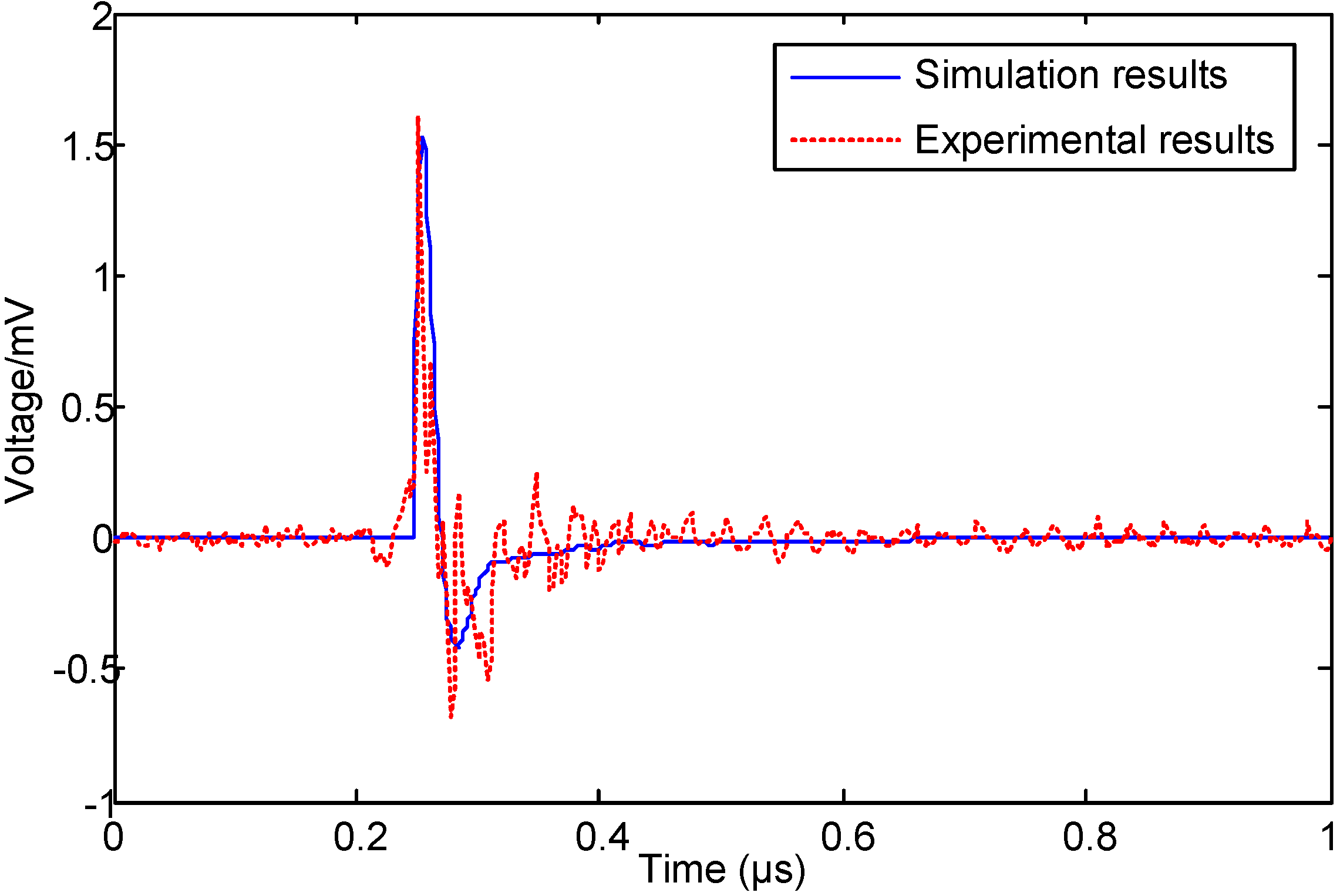
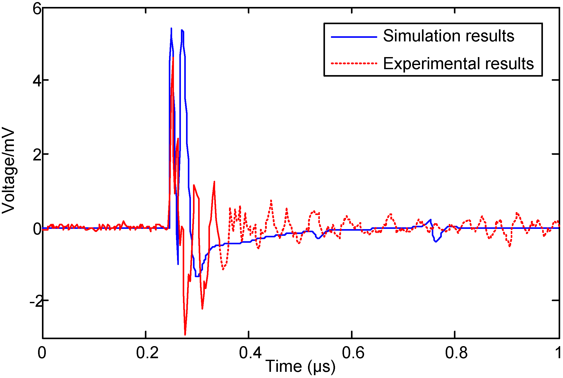
From Figure 3 it can be concluded that the mean square error between the simulation and experiment results are quite small, which means the simulation result is in good accordance with the experimental data. The mean square value reaches its minimum value when the relative permittivity is 2.2 in all cases. Thus the relative permittivity in this model is set as 2.2. The PD current as a response to the 1.2 PDIV of 10 mm needle-sphere electrode configuration is presented and compared with experiment data in Figure 4.

Figure 3. Mean square error analysis.

Figure 3. Mean square error analysis.

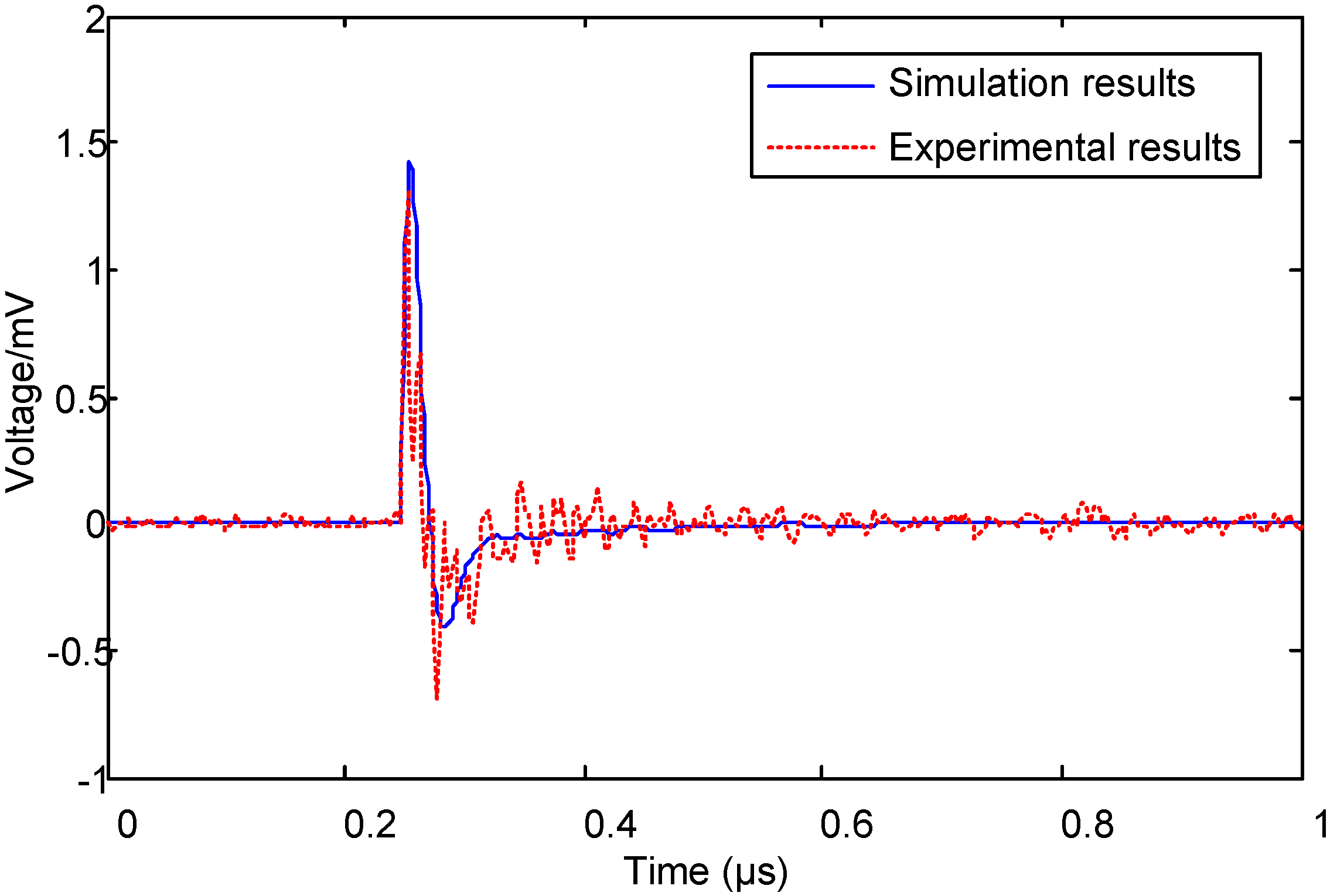
From Figure 4 it can be concluded that despite the noise of the experiment data, the simulation result is in good accordance with the measured PD waveform. However, only the current signal can tell us the macroscopic information of the PD process. With the implementation of the electro-hydrodynamic model, several microscopic characteristics can be assessed.

Figure 4. Comparison of the partial discharge (PD) current between the simulation and experiment as a response to 1.2 PDIV with 10 mm needle-sphere electrode configuration.

Figure 4. Comparison of the partial discharge (PD) current between the simulation and experiment as a response to 1.2 PDIV with 10 mm needle-sphere electrode configuration.

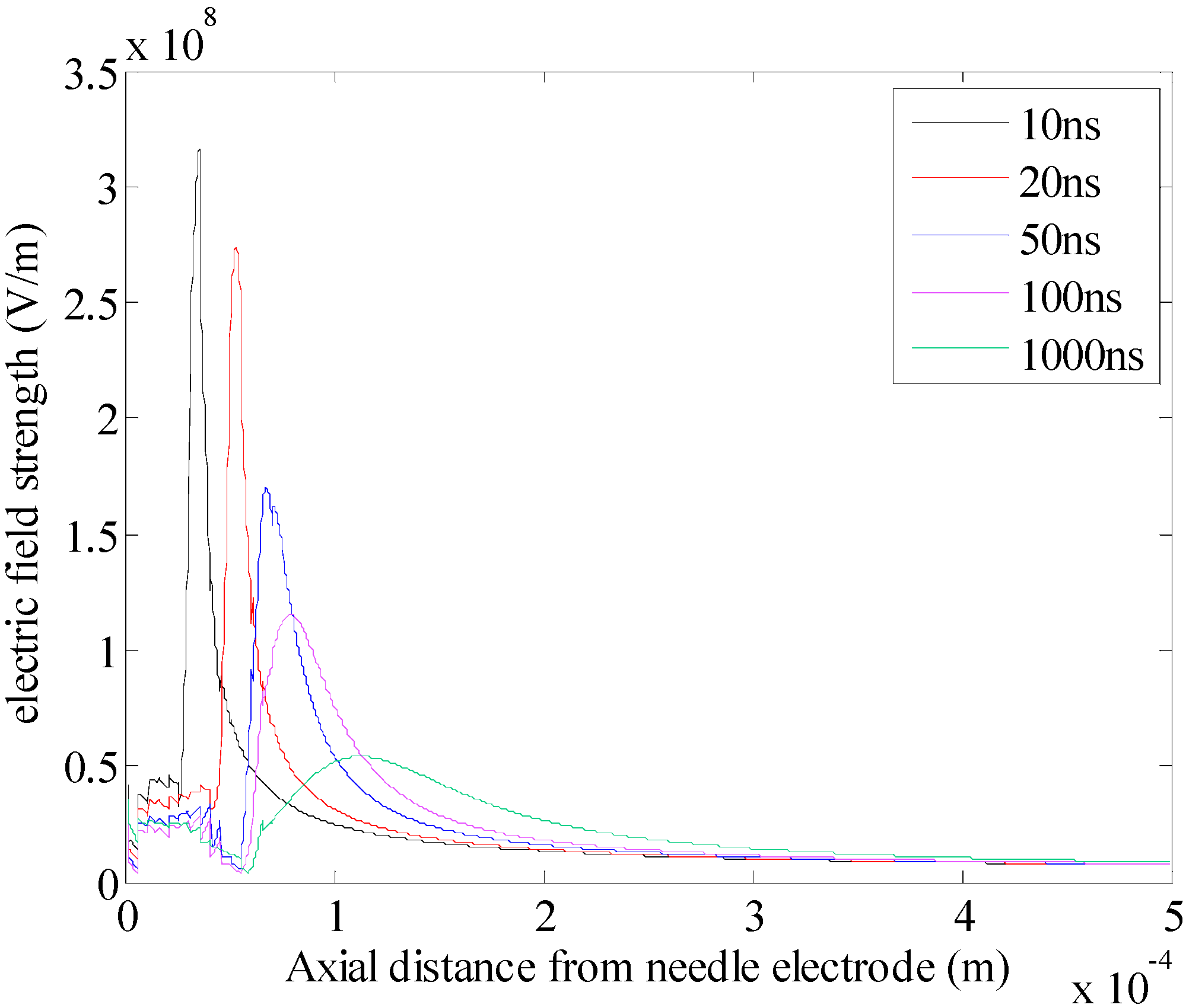
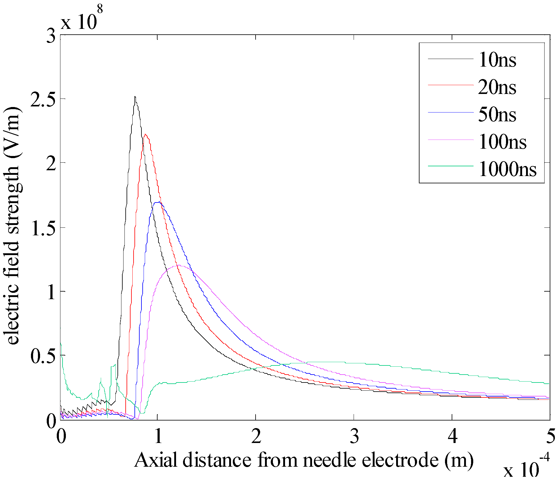
Figure 5 and Figure 6 plot the electric field distribution and potential drop along the electrodes axis. For all time, the peak value of the electric field does not occur at the needle electrode tip as it does for Laplacian field distribution, which means under voltage levels exceeding the PDIV, the space charge generated by the molecule ionization contributes a significant distortion to the original electric field distribution. Also the peak value of the electric field is moving far away from the needle electrode. As the development of PD is a result of the ionization of neutral molecules, the movement of peak value of electric field represents the propagation of the PD.

Figure 5. Electric field distribution along the needle-sphere axis as a response to 1.2 PDIV with 10 mm needle-sphere electrode configuration.

Figure 5. Electric field distribution along the needle-sphere axis as a response to 1.2 PDIV with 10 mm needle-sphere electrode configuration.

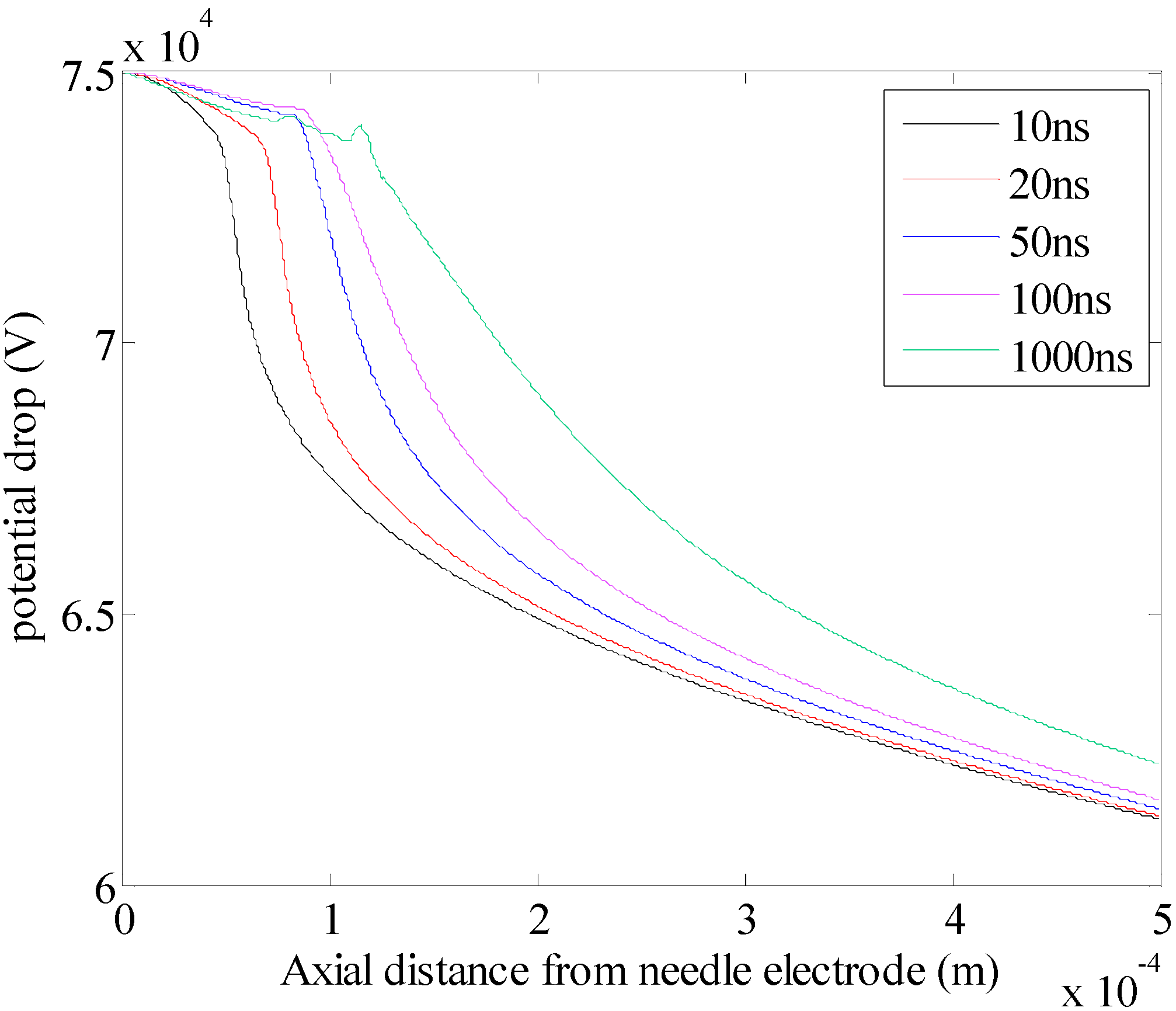
Figure 6. Potential drop along the needle-sphere axis as a response to 1.2 PDIV with 10 mm needle-sphere electrode configuration.

Figure 6. Potential drop along the needle-sphere axis as a response to 1.2 PDIV with 10 mm needle-sphere electrode configuration.

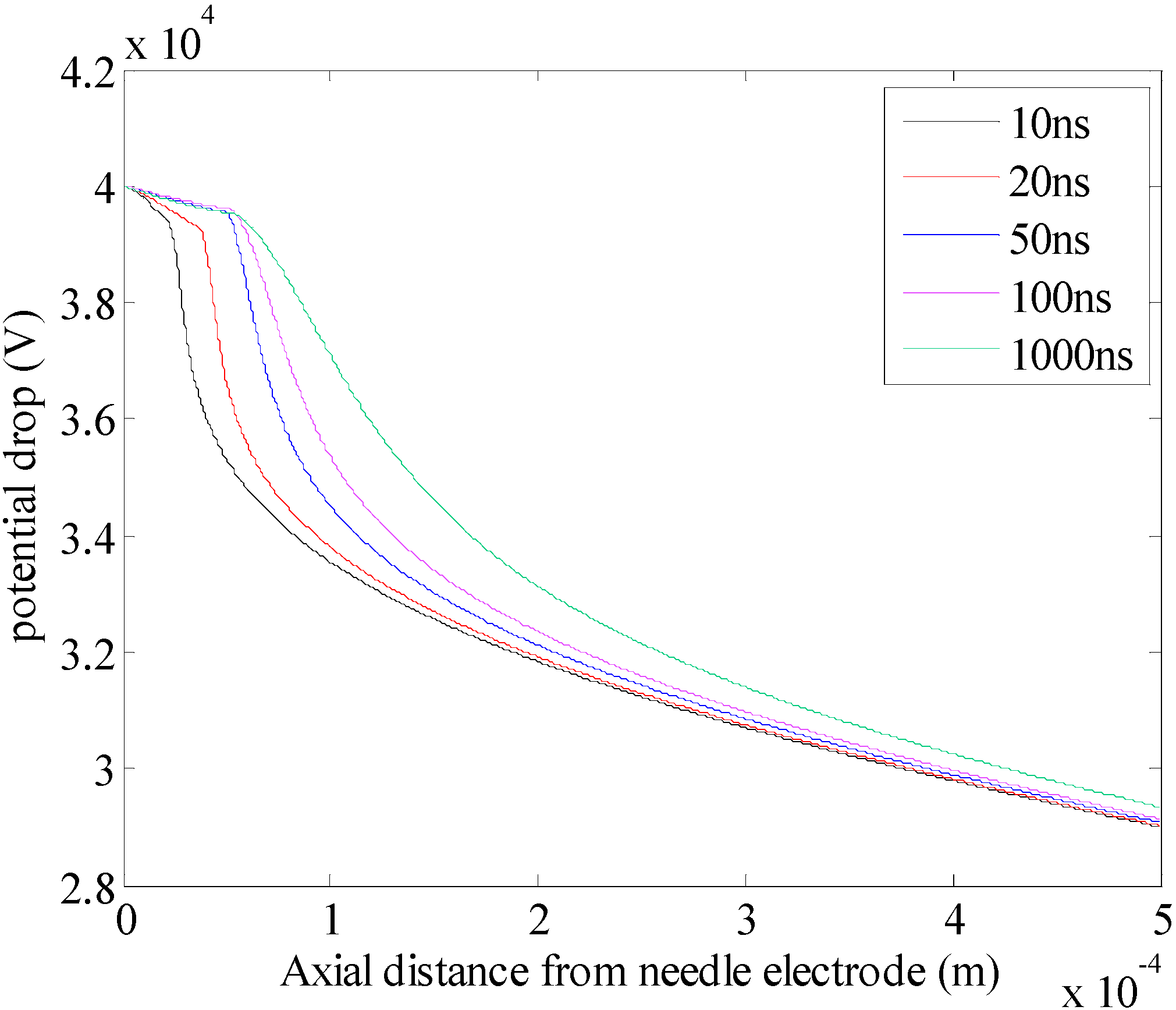
The potential drop is characterized with a flat region near the needle electrode. The potential drop in this region is quite different from the original distribution, which indicates the area affected by the PD process. Also the position of this region is in accordance with the peak value of the electric field.

From the electric field distribution and voltage drop along the axis it can be concluded that the dynamics of the PD process is influenced by both the applied voltage and the space charge generated by the electric field. Space charge is the sum of positive ions, negative ions and electrons. By checking the source and sink term in Equations (1–3) it is obvious that the generation of the negative charge only results from the attachment of the electrons and liquid molecules. However, this process is characterized with a long time scale compared with the collision and recombination process. Thus the negative charge density is quite small compared with those of positive ions and electrons. Also Table 1 shows that the electrons travel with a velocity five orders of magnitude higher than that of positive ions. Additionally, with electric field strength as Figure 5 shows, electrons will quickly sweep over the gap with positive ions remaining almost stationary. Thus the net space charge density is mainly a result of the positive charge density. 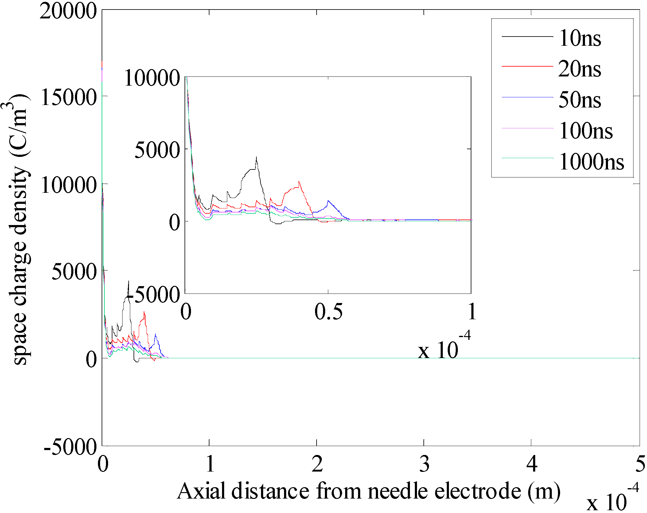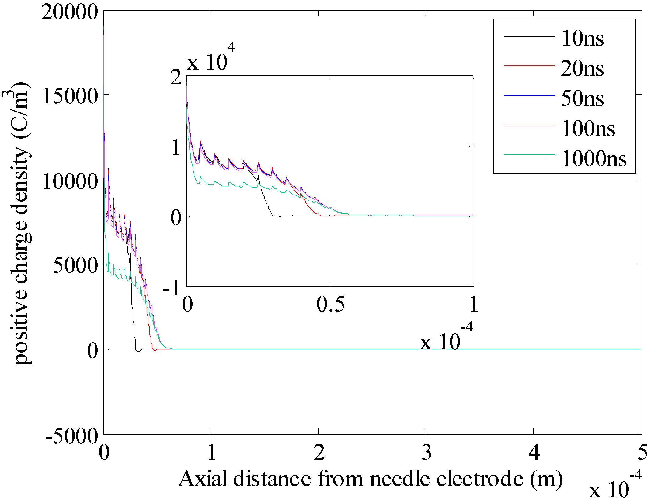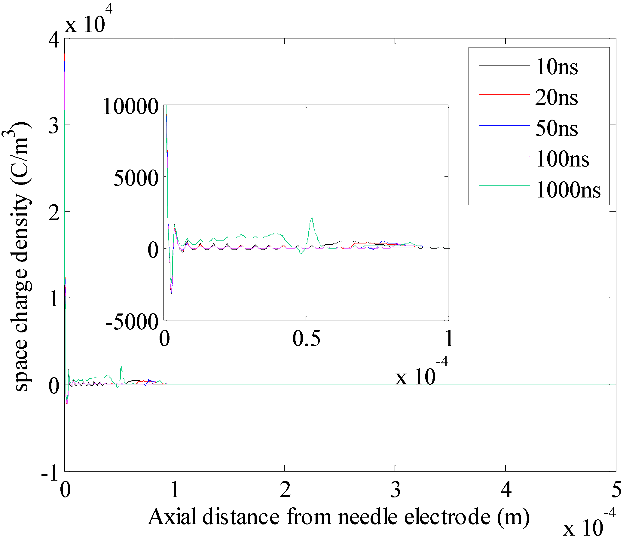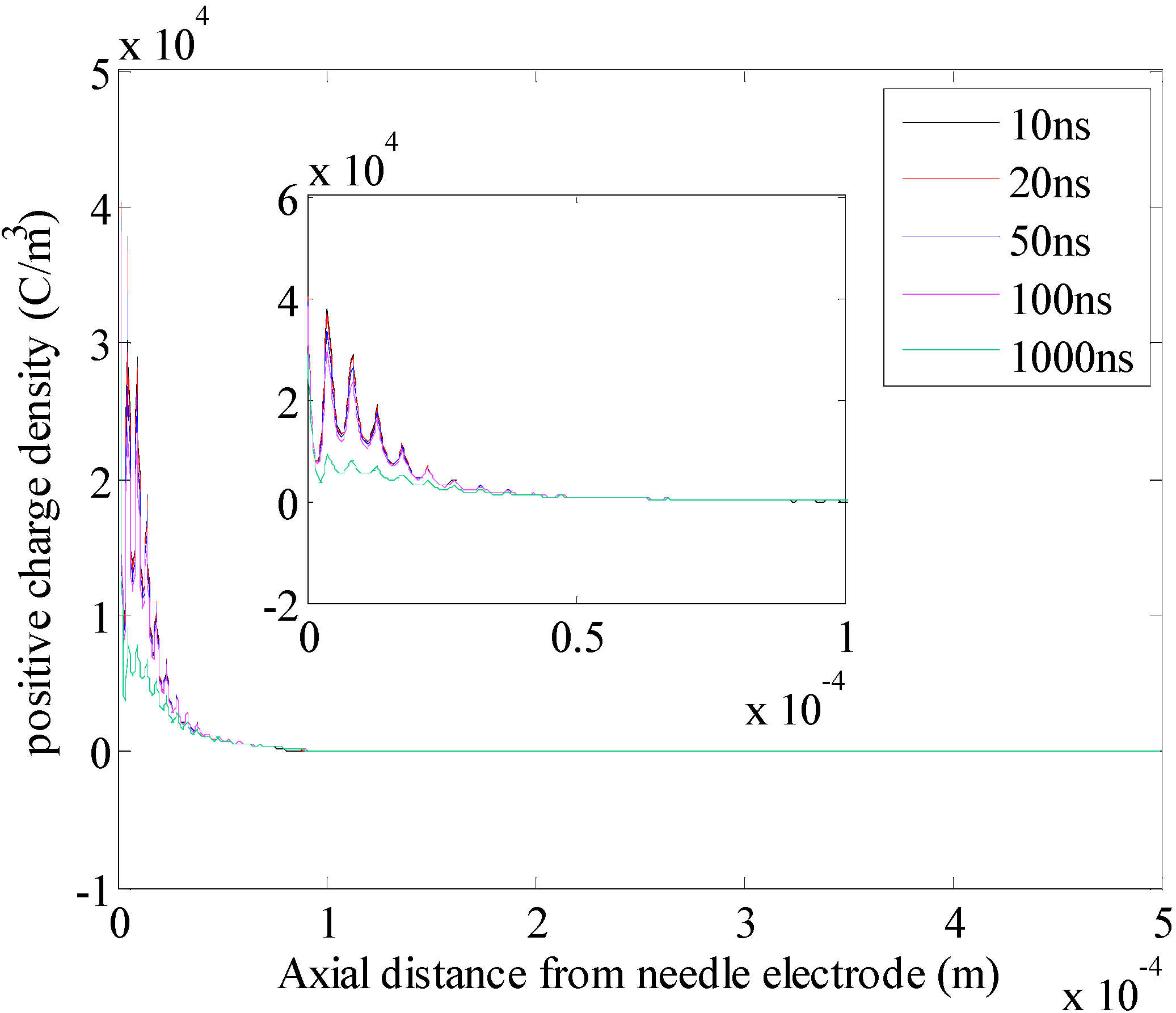Figure 7 and Figure 8 plot the space charge density distribution and positive charge distribution along the needle-sphere axis at time 10, 20, 50, 100 and 1000 ns.

In Figure 7 and Figure 8 the space charge density is characterized with several peaks, which are in the same position with the corresponding peaks of electric field. This means that when the needle electrode is stressed with high voltage, the molecules near the needle tip are ionized. Positive ions and electrons are generated. And these charge carriers are driven to move by the electric field. When the net charge density becomes high enough, it will distort the original Laplacian electric field and the maximum value of the electric field will be a small distance away from the needle tip. After 10 ns, the peak value of space charge and positive charge density start to decay, which represents the decay of the PD current. After 1000 ns, the electric field is so weak that no significant space charge can be generated, and thus the PD current is approximately 0.

Figure 7. Space charge density distribution along the needle-sphere axis as a response to 1.2 PDIV with 10 mm needle-sphere electrode configuration.

Figure 7. Space charge density distribution along the needle-sphere axis as a response to 1.2 PDIV with 10 mm needle-sphere electrode configuration.

Figure 8. Positive charge distribution along the needle-sphere axis as a response to 1.2 PDIV with 10 mm needle-sphere electrode configuration.

Figure 8. Positive charge distribution along the needle-sphere axis as a response to 1.2 PDIV with 10 mm needle-sphere electrode configuration.

5. Effects Influencing the PD Process

Partial discharge is dependent on the applied voltage, gap distance and electrode type. A series of experiments were conducted to study the influence of these parameters. With the implementation of the electro-hydrodynamic model, detailed information concerning the PD process can be obtained.

5.1. Effect of Amplitude of Applied Voltage

The amplitude of applied voltage determines the Laplacian electric field distribution in the bulk of the liquid. With the same electrode geometry and gap distance, higher applied voltage will lead to a more intense electric field, and thus a different PD process. It is important to study the influence of applied voltage on the PD process. In order to get reliable PD events and compare with the 1.2 PDIV case, 1.5 PDIV is implemented in the 10 mm gap experiments. The comparison between the experimental data and simulation results is plotted in Figure 9.

Figure 9. Comparison of the PD current between the simulation and experiment as a response to 1.5 PDIV with 10 mm needle-sphere electrode configuration.

Figure 9. Comparison of the PD current between the simulation and experiment as a response to 1.5 PDIV with 10 mm needle-sphere electrode configuration.

It can be concluded that the PD current under 1.5 PDIV is higher than 1.2 PDIV. This is in accordance with the fact that with higher applied voltage, the Laplacian field will be higher. Thus more space charge will be generated and move into the electrodes. The amplitude of the 1.5 PDIV case is more than (1.5/1.2) orders of magnitude larger than the 1.2 PDIV case, which means the increment of applied voltage and the current is in a superliner relationship. This is because that the electric field distribution is the result of the combined effect of applied voltage and the space charge generated by the ionization of liquid molecules, which will distort the original Laplacian field. Figure 10 and Figure 11 show the electric field distribution and potential drop between the two electrodes along the needle-sphere axis at time 10, 20, 50, 100 and 1000 ns.

Figure 10. Electric field distribution along the needle-sphere axis as a response to 1.5 PDIV with 10 mm needle-sphere electrode configuration.

Figure 10. Electric field distribution along the needle-sphere axis as a response to 1.5 PDIV with 10 mm needle-sphere electrode configuration.

Figure 11. Potential drop along the needle-sphere axis as a response to 1.5 PDIV with 10 mm needle-sphere electrode configuration.

Figure 11. Potential drop along the needle-sphere axis as a response to 1.5 PDIV with 10 mm needle-sphere electrode configuration.

For the 1.5 PDIV case, the peak of the electric field travels with a higher velocity and with the same interval of time, it can cover a larger range than the 1.2 PDIV case. Also its peak value is decreasing with a slightly smaller rate.

By checking the potential drop along the axis, the difference between the two cases is more obvious. Within the same range of distance from the needle electrode, the potential drop decreases from 6 × 10⁴ V to approximately 4.9 × 10⁴ V for 1.2 PDIV case. For 1.5 PDIV case, the voltage drop is from 7.5 × 10⁴ V to approximately 6.2 × 10⁴ V.

Figure 12 and Figure 13 plot the space charge density distribution and positive charge distribution along the needle-sphere axis at time 10, 20, 50, 100 and 1000 ns.

Figure 12. Space charge density distribution along the needle-sphere axis as a response to 1.5 PDIV with 10 mm needle-sphere electrode configuration.

Figure 12. Space charge density distribution along the needle-sphere axis as a response to 1.5 PDIV with 10 mm needle-sphere electrode configuration.

Figure 13. Positive charge density distribution along the needle-sphere axis as a response to 1.5 PDIV with 10 mm needle-sphere electrode configuration.

Figure 13. Positive charge density distribution along the needle-sphere axis as a response to 1.5 PDIV with 10 mm needle-sphere electrode configuration.

By comparing the 1.2 PDIV and 1.5 PDIV cases, it is obvious that the amplitudes of both space charge density and positive charge density in the 1.5 PDIV case are greater than those in the 1.2 PDIV one. This result can be predicted from the electric field distribution. In 1.5 PDIV case, the electric field strength is stronger and covers a wider area.

From Figure 12 it can be concluded that the net space charge near the anode is positive, which means the electric field strength at the tip of the PD channel will be increased, leading more molecules to be ionized in front of the PD channel. This means higher space charge density resulting from higher applied voltage tends to sustain a further PD development. In other words, the space charge PD process in the 1.2 PDIV case are restricted in a more localized region than 1.5 PDIV case.

As the electric field and space charge distribution both cover a larger range in the 1.5 PDIV case than in the 1.2 PDIV case, there will be more charge carriers sweeping into the electrode in the 1.5 PDIV case. Thus the leakage current calculated using Equation (8) will be characterized with higher amplitude in the 1.5 PDIV case than that in the 1.2 PDIV case. At the same time, it should be noticed that the generation rate of the charge carriers is not increasing linearly with the electric field strength, thus it explains why the current has a superliner relationship with increment of the applied voltage.

5.2. Effect of Gap Distance

In on-site measurement, the PDIV level is dependent on the geometry of the defect. In this study, in order to check the effect of gap distance on the PD process, 5 mm and 10 mm gap distance are implemented. The applied voltages are selected as 1.2 PDIV for the corresponding gap distance. Figure 14 plots the Comparison of the PD current between the simulation and experiment as a response to 1.2 PDIV with 5 mm needle-sphere electrode configuration.

It can be concluded from Figure 14 that with the same PDIV level, the waveform of the PD currents for 5 mm and 10 mm gap distances are very similar with each other. The amplitude of the PD current for 10 mm gap distance is slightly larger than that for 5 mm gap distance.

Figure 14. Comparison of the PD current between the simulation and experiment as a response to 1.2 PDIV with 5 mm needle-sphere electrode configuration.

Figure 14. Comparison of the PD current between the simulation and experiment as a response to 1.2 PDIV with 5 mm needle-sphere electrode configuration.

Figure 15 and Figure 16 show the electric field distribution and potential drop between the two electrodes along the needle-sphere axis at time 10, 20, 50, 100 and 1000 ns. At 10 ns and 20 ns, the electric field strength for the 10 mm gap is higher than that for the 5 mm gap. At 100 ns and 1,000 ns, the electric field distributions for both cases are almost the same. At each time, the position of the peak value of the electric field for both cases is almost the same. As for the potential drop, despite the difference of the value, the patterns of the two cases are in good accordance with each other.

Figure 15. Electric field distribution along the needle-sphere axis as a response to 1.2 PDIV with 5 mm needle-sphere electrode configuration.

Figure 15. Electric field distribution along the needle-sphere axis as a response to 1.2 PDIV with 5 mm needle-sphere electrode configuration.

Figure 16. Potential distribution along the needle-sphere axis as a response to 1.2 PDIV with 5 mm needle-sphere electrode configuration.

Figure 16. Potential distribution along the needle-sphere axis as a response to 1.2 PDIV with 5 mm needle-sphere electrode configuration.

Figure 17 and Figure 18 show the space charge density and positive charge density distribution between the two electrodes along the needle-sphere axis at time 10, 20, 50, 100 and 1000 ns. Similar with the electric field distribution, the space charge density and positive charge density distribution for 10 mm cases are higher than those for 5 mm cases at 10 ns and 20 ns.

From Figure 17 and Figure 18 it can be concluded that with the same PDIV level, the PD process for different gap distances is quite similar. Based on previous research, PDIV has a superliner relation with the increase of the geometry. Thus with a longer gap distance, the initial electric field will be higher, and at first stage, the PD current is larger for the longer gap distance. This is in accordance with the fact that with larger discharge areas, the PD process will be more intense even with the same PDIV level. However with the generation of space charge, the electric field distribution is distorted and will gradually become the same for different gap distance, and consequently lead to similar PD current.

Figure 17. Space charge density distribution along the needle-sphere axis as a response to 1.2 PDIV with 5 mm needle-sphere electrode configuration.

Figure 17. Space charge density distribution along the needle-sphere axis as a response to 1.2 PDIV with 5 mm needle-sphere electrode configuration.

Figure 18. Positive charge density distribution along the needle-sphere axis as a response to 1.2 PDIV with 5 mm needle-sphere electrode configuration.

Figure 18. Positive charge density distribution along the needle-sphere axis as a response to 1.2 PDIV with 5 mm needle-sphere electrode configuration.

5.3. Effect of Electrode Configuration

The needle-sphere electrode is a typical configuration which will lead to non-uniform electric field distribution along the needle-sphere axis. It represents the spindle-shaped defect. The electric field near both electrodes will be stronger than the field within the middle of the gap. The electric field distribution along the needle-sphere axis is in a U shape, which means both the generation rate and the velocity of charge carriers will be higher in the region near both electrodes than in the gap middle. A needle-plate electrode configuration is another kind of electrode set up which will lead to non-uniform electric field distribution. It represents a cone-shaped defect. Electric field strength near the needle electrode is very strong and decreases rapidly along the axis. Experiments and simulations have been conducted to study the PD characteristics resulting from different electrode configurations. The stressed electrode remains the same while the earthed sphere electrode is replaced with a plate electrode with a radius of 5 mm. The applied voltage is 1.2 PDIV.

Figure 19 plots the PD current of needle-plate electrode geometry. It can be concluded that the PD current of the needle-plate electrode is significantly higher than that of the needle-sphere electrode. Also after the PD current reaches its peak value, it decreases with a slower rate comparing with the needle-sphere electrode. Figure 20 and Figure 21 show the electric field distribution between the two electrodes along the needle-sphere axis at time 10, 20, 50, 100 and 1000 ns.

Interestingly, although the PD current is larger for the needle-plate electrode, the peak value of the electric field distribution at each time is smaller than that of the needle-sphere electrode. However the curve of electric field distribution for the needle-plate electrode is flatter. By checking the potential drop along the electrode axis, the potential drops from 5.5 × 10⁴ V to approximately 3.5 × 10⁴ V within 0.5 mm for the needle-plate case, while for the needle-sphere case the potential difference within the same distance is less than 1.2 × 10⁴ V. The potential drop is the integration of the electric field strength along a certain distance. Thus it can be concluded that although the peak value of the electric field for the needle-plate electrode is smaller than that of the needle-sphere electrode, its distribution is flatter and consequently can influence a wider area.

Figure 19. Comparison of the PD current between the simulation and experiment as a response to 1.2 PDIV with 10 mm needle-plate electrode configuration.

Figure 19. Comparison of the PD current between the simulation and experiment as a response to 1.2 PDIV with 10 mm needle-plate electrode configuration.

Figure 20. Electric field distribution along the needle-sphere axis as a response to 1.2 PDIV with 10 mm needle-plate electrode configuration.

Figure 20. Electric field distribution along the needle-sphere axis as a response to 1.2 PDIV with 10 mm needle-plate electrode configuration.

Figure 21. Potential distribution along the needle-sphere axis as a response to 1.2 PDIV with 10 mm needle-plate electrode configuration.

Figure 21. Potential distribution along the needle-sphere axis as a response to 1.2 PDIV with 10 mm needle-plate electrode configuration.

Figure 22 and Figure 23 show the space charge density and positive charge density distribution between the two electrodes along the needle-sphere axis at time 10, 20, 50, 100 and 1000 ns. As a result of the electric field distribution, the space charge density and positive charge density distribution for needle-plate electrodes are higher than those for needle-sphere electrodes. Also their distribution covers a wider area.

Figure 22. Space charge density distribution along the needle-sphere axis as a response to 1.2 PDIV with 10 mm needle-plate electrode configuration.

Figure 22. Space charge density distribution along the needle-sphere axis as a response to 1.2 PDIV with 10 mm needle-plate electrode configuration.

Figure 23. Positive charge density distribution along the needle-sphere axis as a response to 1.2 PDIV with 10 mm needle-plate electrode configuration.

Figure 23. Positive charge density distribution along the needle-sphere axis as a response to 1.2 PDIV with 10 mm needle-plate electrode configuration.

Thus it can be concluded that for the needle-plate electrode geometry, its peak value of electric field is smaller than that of the needle-sphere electrode. However, as its electric field distribution is flatter, it can influence a wider area, and within this area, more space charge will be generated. Therefore the discharge current is characterized with larger amplitude.

6. Conclusions

This paper presents a study concerning the factors influencing the partial discharge process in liquid dielectrics. Experiments have been conducted to study the effects of amplitude of applied voltage, gap distance, and electrode type on the PD process. An electro-hydrodynamic model describing the dynamics of charge carriers has been implemented to generate the simulation data. This model is validated through the comparison between the simulation results and experimental data of the PD current. With the implementation of this model, the effects of amplitude of applied voltage, gap distance, and electrode type on the PD process are studied. Analysis based on the simulation results explains the mechanism of how these factors affect the PD process. The results may be summarized as follows:

(1) For higher amplitude of applied voltage, the Laplacian electric field strength will be stronger. The space charge will increase in a superliner relationship with the electric field, which will enhance the electric field in front of the PD channel. Thus the peak value of the PD current will be higher for higher amplitude of applied voltage, and the PD process will cover a larger area.

(2) The PDIV has a superliner relationship with the gap distances. For longer gap distance with the same PDIV level, the original electric field will be the stronger. Thus the peak value of the PD current is higher for longer gap distances. However, with the decay of the PD current, the generation of new charge carriers cannot distort the electric field distribution and thus the PD current will gradually become the same.

(3) The needle-plate electrode configuration will lead to a flatter electric field distribution near the needle electrode compared to the needle-sphere arrangement. Although the peak value of the electric field is smaller than that of the needle-sphere electrode, with its flatter distribution, more space charge can be generated within the same area. Thus the PD current will be higher for the needle-plate electrode geometry with the same PDIV level than the needle-sphere electrode.