Application of Coordinated SOFC and SMES Robust Control for Stabilizing Tie-Line Power

Abstract

Wind power causes fluctuations in power systems and introduces issues concerning system stability and power quality because of the lack of controllability of its discontinuous and intermittent resources. This paper presents a coordinated control strategy for solid oxide fuel cells (SOFCs) and superconducting magnetic energy storage (SMES) to match the intermittent wind power generation and compensate for the rapid load changes. An optimal H∞ control method, where the weighting function selection is expressed as an optimization problem, is proposed to mitigate tie-line power fluctuations and the mixed-sensitivity approach is used to deal with the interference suppression. Simulation results show that the proposed method significantly improves the smoothing effect of wind power fluctuations. Compared with the conventional control method, the proposed method has better anti-interference performance in various operating situations.

1. Introduction

Recently, wind power has been increasingly applied in power systems because of its environmental benefits. However, wind power fluctuations also cause problems in power system operation [1,2,3]. Therefore, several studies on wind power control are required for effective wind power generation.

In more recent years, the complementarities between storage and renewable energy sources (RESs) have recently become of particular interest, both in terms of essentially intermittent resources and stability maintenance in electrical power systems [4,5]. Both RESs and storage have different characteristics. Thus, the type and capacity of energy storage to be used must be carefully selected. Energy storage systems must have either fast response parts or a certain amount of energy storage capacity to meet the demands of load and generation adjustments and to improve the performance of RESs [6]. A single energy storage device cannot satisfy these requirements. Therefore, a composite energy storage system is necessary [7,8]. In this paper, solid oxide fuel cells (SOFCs) are used to supply the basic load to deal with the discontinuous and intermittent wind power fluctuations. However, SOFCs cannot adequately compensate sudden load changes and instantaneously smooth severe wind power fluctuations because of their slow dynamic response [9,10,11]. Thus, a superconducting magnetic energy storage (SMES) system, which can act as a good tool for considerably decreasing the power fluctuations of the wind generator system, was used [12,13,14,15,16,17,18]. The overall control of the microgrid power system was performed using the control and monitoring system (CMS) [6].

This paper proposes a new robust design of coordinated SOFC and SMES controllers for smoothing wind power fluctuations. An optimal H∞ control method [19,20], where the weighting function selection is expressed as an optimization problem [21,22], is proposed to mitigate tie–line power fluctuations. And the mixed-sensitivity approach is used to deal with the interference suppression [23,24,25]. This study primarily aims to mitigate and smooth the tie-line power deviation using the proposed control strategy.

The remainder of the paper is organized as follows: Section 2 briefly describes the microgrid system and establishes the SOFC and SMES models. Section 3 illustrates the proposed H∞ mixed-sensitivity design based on PSO [26,27,28]. Section 4 shows the simulation results from different cases and compares the performances of different control strategies. Section 5 reviews the proposed control strategy and concludes this paper.

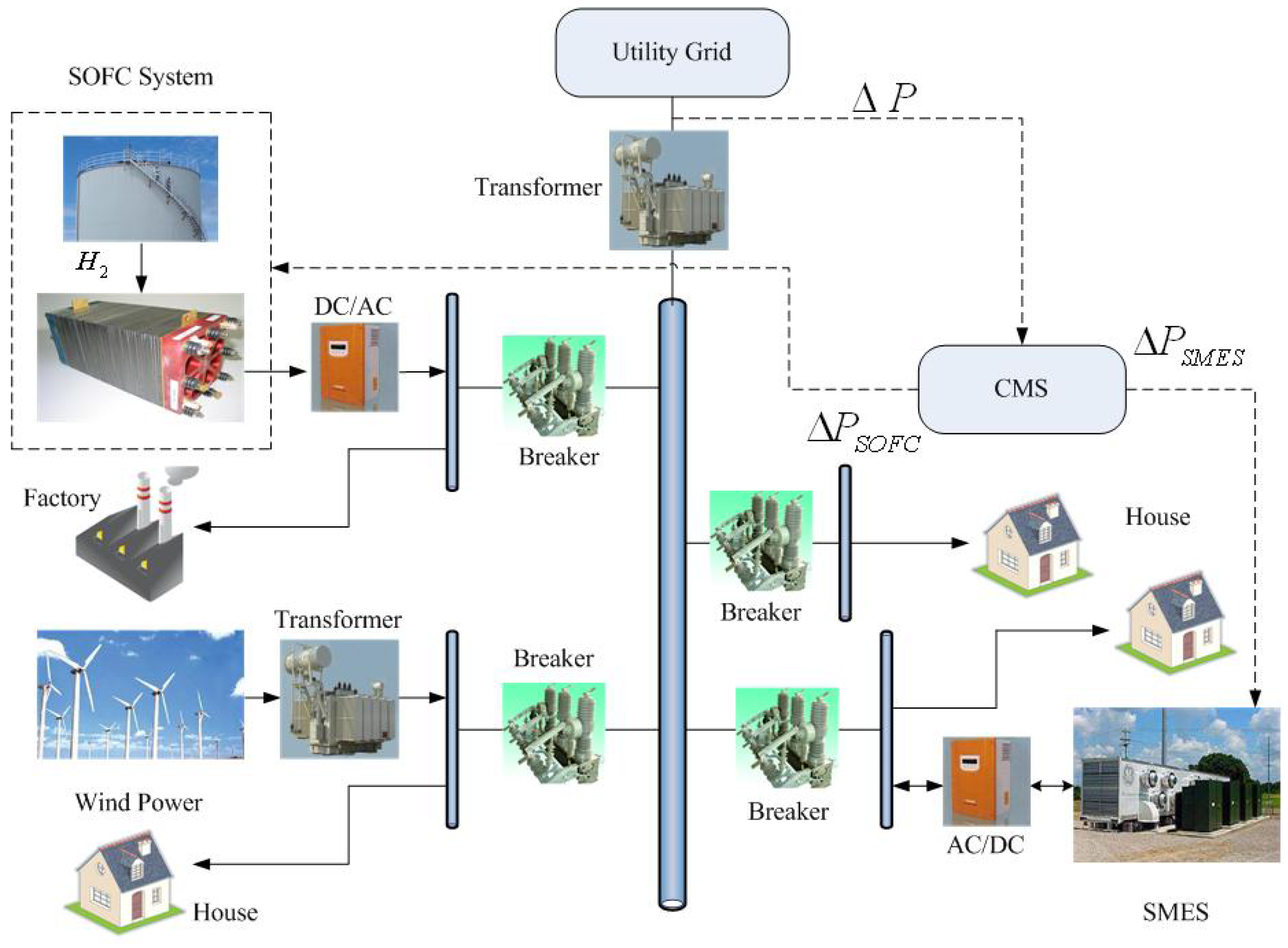
2. Microgrid Model

A microgrid is an interconnection of distributed energy sources integrated with storage devices and power capacitors on low-voltage distribution systems. Figure 1 shows the basic microgrid architecture.

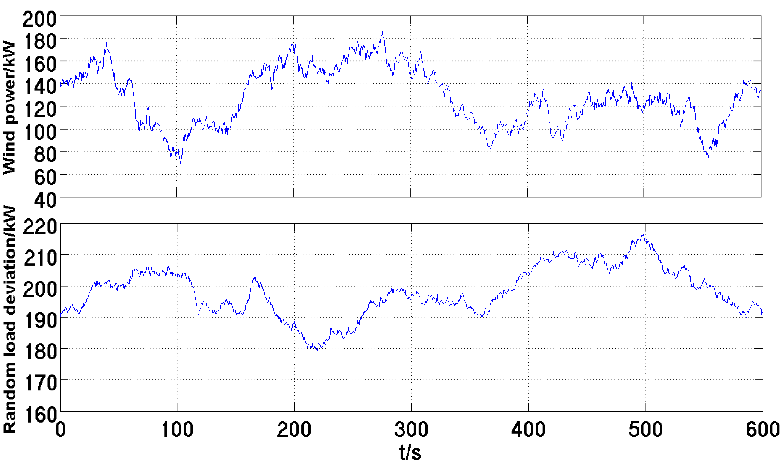
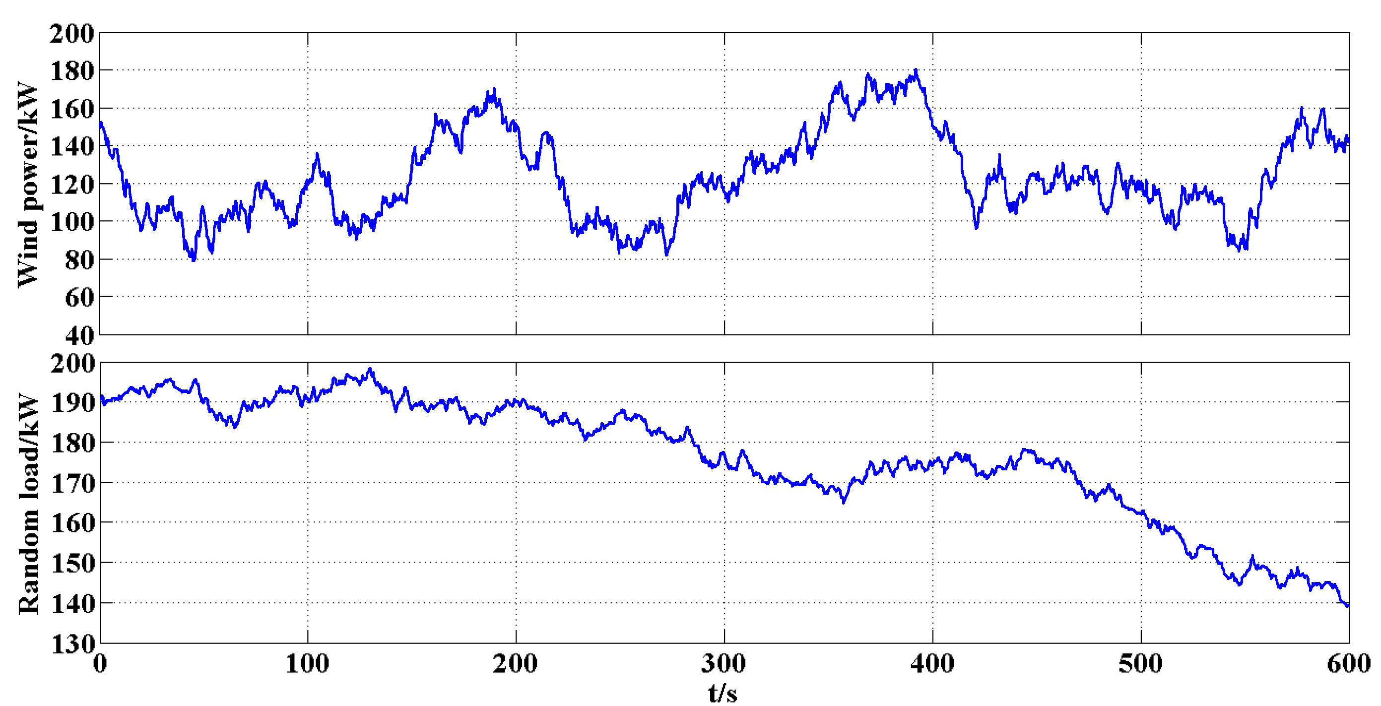
2.1. Wind Power and Load Models

Wind power, which is the primary power source, provides power to the load according to different power demand levels. The SOFC supplies additional power to the microgrid system when the wind power is insufficient, and the SMES stabilizes tie-line power fluctuations. In this paper, the standard deviations of wind power PWP and random load deviation P_Load were mathematically evaluated as follows [6]:

$$d{P}_{WP}=0.8\sqrt{P_{WP}}$$

(1)

$$d{P}_{Load}=0.6\sqrt{P_{Load}}$$

(2)

As shown in [7,8], the wind power fluctuation is derived from white noise, and a low-pass filter is used to eliminate components that are higher than 10,000 s. Then, the fluctuation is multiplied by the standard deviation to determine the output fluctuation. On the other hand, the load fluctuation is generated similarly. Low- and high-pass filters are used to eliminate components that are lower than 5 min and higher than 30 min, respectively. The fluctuation is then multiplied by the standard deviation and base load capacity to determine the output fluctuation.

Figure 1. Microgrid system.

Figure 1. Microgrid system.

Wind power output and random load deviation in Figure 2 are employed in the microgrid system under grid-connected operation.

Figure 2. Wind power output and random load deviation.

Figure 2. Wind power output and random load deviation.

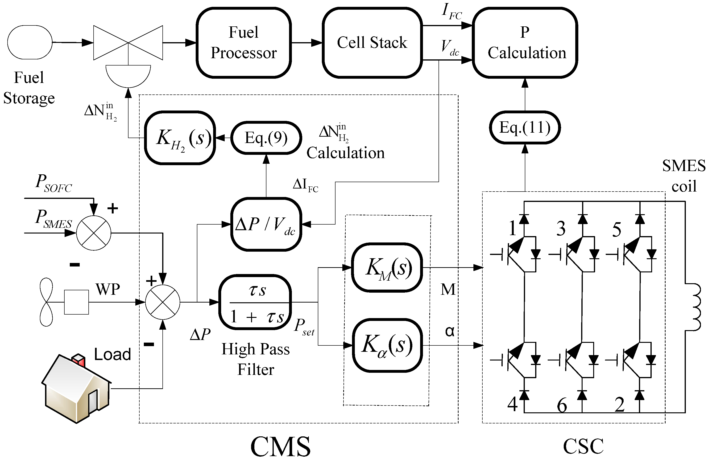
2.2. SOFC Models

The SOFC model used in this paper was established by Padullés et al. [9,10]. The operating temperature of the FC is assumed constant, and the drop in the FC electromotive force (EMF) due to ohmic loss is considered. The electrochemical and thermodynamic processes were approximated using first-order transfer functions [9,11].

Ideally, SOFC differential equations are established as follows:

$$\frac{d}{dt}{p}_{H_2}=\frac{1}{{\tau }_{H_2}{K}_{H_3}}(N_{H_2}^{in}-K_{H_2}{P}_{H_2}-2K_{r}I)$$

(3)

$$\frac{d}{dt}{p}_{O_2}=\frac{1}{{\tau }_{O_2}{K}_{O_3}}(N_{H_2}^{in}/r_{H-O}-K_{O_2}{P}_{O_2}-K_{r}I)$$

(4)

$$\frac{d}{dt}{p}_{H_{2}O}=\frac{1}{{\tau }_{H_{2}O}{K}_{H_2{O}_3}}(N_{H_{2}O}^{in}-K_{H_{2}O}{P}_{H_{2}O}+2K_{r}I)$$

(5)

where P_H2, P_O2 and P_H2O (atm) and K_H2, K_O2 and K_H2O [mol/(s·atm)] are the partial pressures and valve molar constants for hydrogen, oxygen, and water, respectively; and τ_H2, τ_O2 and τ_H2O are the time constants of the three kinds of gas flows; K_r is a modeling parameter with a value of N₀/4F mol/s·A; N₀ is the number of stack cells in series, and F is the Faraday constant (96,487 C/mol).

The well-known Nernst equation was used to calculate the internal EMF generated by the FC stack, as Equation (6):

$$V=N_0\left[E_0+\frac{RT}{2F}ln\left(\frac{p_{H_2}{p}_{O_2}^{0.5}}{p_{H_{2}O}}\right)\right]-rI$$

(6)

where R is the gas constant (8.31 J/mol·K); T is the SOFC typical operating temperature; E₀ is the voltage associated with the reaction free energy (V); and r denotes the ohmic losses of the stack (Ω).

The utilization factor [11] of the SOFC is defined as follows:

$$u\equiv (N_{H_2}^{in}-N_{H_2}^{out}){/N}_{H_2}^{in}$$

(7)

According to [9], the term u can be expressed as follows:

$$I_{FC}=u\cdot N_{H_2}^{in}/2K_r$$

(8)

Considering the fuel processor dynamics, the relationship between the small changes in the stack current ΔI_FC and hydrogen input $\Delta N_{H_2}^{in}$ fed to the FC stack can be derived as:

$$\Delta I_{FC}=\frac{u/2K_r}{{\tau }_{f}s+1}\Delta N_{H_2}^{in}$$

(9)

A linear SOFC model can be obtained at the nominal operating point using the Jacobian linearization. At the nominal operating point, I_FC = 200 A and V = 400 V.

2.3. SMES Models

The SMES is a large superconducting coil capable of storing electric energy in the magnetic field generated by the dc current flowing through it [12]. Though the installation of SMES is quite costly [13], SMES systems have attracted much attention because of their fast response and high efficiency.

SMES modeling largely depends on the converter topology and control method [14]. In this paper SMES device is connected to two parallel current source converters (CSCs) to reduce the harmonics and expand the active and reactive power regulation ranges [15,16]. Equally triggering angle control of the CSC ensures that the SMES device performs the active and reactive power decoupling control. In this structure, its control mode can be mapped into the modulation index M and triggering angle α. According to [16], first-order transfer equations are assumed to control M and α as follows:

$$\{\begin{array}{c}\stackrel{•}{M}=-\frac{1}{T_{\ast }}M+\frac{1}{T_{\ast }}{u}_1\\ \stackrel{•}{\alpha }=-\frac{1}{T_{\ast }}\alpha +\frac{1}{T_{\ast }}{u}_2\end{array}$$

(10)

$$\{\begin{array}{c}P=1.5M{V}_{\max }{I}_d\cos \alpha \\ Q=1.5M{V}_{\max }{I}_d\sin \alpha \end{array}$$

(11)

where P and Q are the active and reactive powers that flow to the SMES, respectively; V_max is the maximum system voltage of the access point; I_d is the superconducting coil current; $T_{*}$ is the time constant of the converter; and u₁ and u₂ are the control variables of M and α, respectively:

$$\stackrel{•}{P}=1.5\stackrel{•}{M}{V}_{\max }{I}_d\cos \alpha +1.5M{V}_{\max }{I}_d(\sin \alpha )\cdot \stackrel{•}{\alpha }=-\frac{1}{T_{\ast }}P+\frac{1}{T_{\ast }}(Q\alpha +\frac{P}{M}{u}_1-Q{u}_2)$$

(12)

Similarly:

$$\stackrel{•}{Q}=-\frac{1}{T_{\ast }}Q+\frac{1}{T_{\ast }}(-P\alpha +\frac{Q}{M}{u}_1+P{u}_2)$$

(13)

Considering system uncertainties, an interference function ω is introduced into the state equation as Equation (14):

$$\begin{array}{c}\{\begin{array}{c}\stackrel{•}{x}=Ax+B_{1}u+B_{2}w\\ z=C_{1}x+D_{11}u+D_{12}w\\ y=C_{2}x+D_{21}u+D_{22}w\end{array}\\ A=\left[\begin{array}{cccc}-\frac{1}{T_{\ast }}& & & \\ & -\frac{1}{T_{\ast }}& & \\ & \frac{Q}{T_{\ast }}& -\frac{1}{T_{\ast }}& \\ & -\frac{P}{T_{\ast }}& & -\frac{1}{T_{\ast }}\end{array}\right]B=\left[\begin{array}{cccc}\frac{1}{T_{\ast }}& & & \\ & \frac{1}{T_{\ast }}& & \\ \frac{P}{M{T}_{\ast }}& -\frac{Q}{T_{\ast }}& 1& \\ \frac{Q}{M{T}_{\ast }}& \frac{P}{T_{\ast }}& & 1\end{array}\right]C=\left[\begin{array}{cccc}0& 0& 1& 0\\ 0& 0& 0& 1\\ 0& 0& 1& 0\\ 0& 0& 0& 1\end{array}\right]D=\left[\begin{array}{cccc}0& 0& -1& 0\\ 0& 0& 0& -1\\ 0& 0& -1& 0\\ 0& 0& 0& -1\end{array}\right]\end{array}$$

(14)

where the state variables x = [M, α, P, Q]^T; control variables u = [u₁, u₂]^T; z and y are the system output signals; w = [P_set , Q_set]^T; and y = [P−P_set, Q−Q_set]^T.

Considering that the SMES device works around the zero point, the state equation can be linearized to obtain the robust linear four-order SMES model. The time constant of converter transfer function $T_{*}$ is 2 ms.

The energy stored in the SMES E (J) and the initial energy stored E₀ (J) can be determined by [17,18]:

$$E_0=0.5L{I}_0^2$$

(15)

$$E=E_0-E_{out}$$

(16)

where I₀ is the actual value of initial coil current (A); the coil inductance of SMES, L is set at 3.3H; E_out is the energy output (J):

$$E_{out}={\displaystyle \int P_{out}dt}$$

(17)

$$I_d=\sqrt{I_0^2-\frac{2E_{out}}{L}}$$

(18)

Subsequently, the coil current I_d can be calculated.

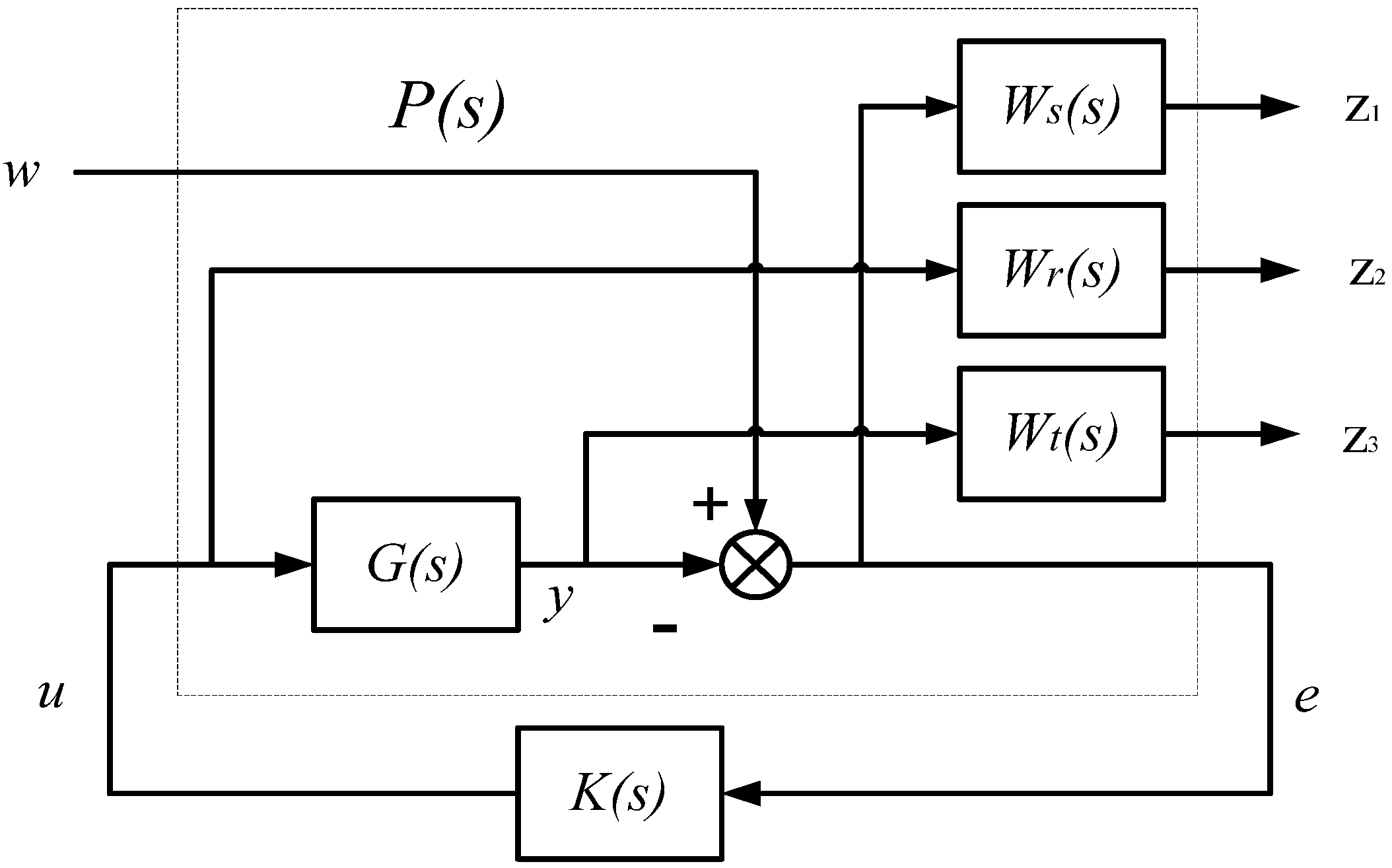
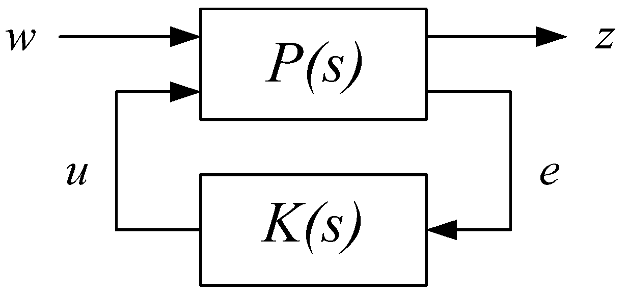
3. H_∞ Optimal Control

3.1. H_∞ Mixed-Sensitivity Problem

Usually, unstructured system uncertainties and external disturbances simultaneously appear in practical control engineering frameworks [19]. Different weighting functions are introduced into the mixed-sensitivity H_∞ design to determine the performance and robustness of the control objectives [20].

Many alternative methods can be used to obtain the generalized plant P(s) in the S/KS/T mixed-sensitivity problem [21,22]. Figure 3 shows the configuration of the generalized plant. W_s(s), W_r(s) and W_t(s) denote the respective weighting functions, which specify the range of relevant frequencies for the corresponding closed-loop transfer matrix, and construct the generalized plant P(s) together with the nominal model G(s) [23,24]. K(s), u, e, w and z denote the controller, control signal, measured variable, external disturbance signal, and so-called error variable, respectively.

Figure 3. Mixed-sensitivity configuration.

Figure 3. Mixed-sensitivity configuration.

The generalized plant P(s) can be described as follows:

$$P(s)=\left[\begin{array}{c}{W}_s\\ 0\\ 0\\ I\end{array}\begin{array}{c}\\ \\ \\ \end{array}\begin{array}{c}-W_{s}G\\ W_r\\ W_{t}G\\ -G\end{array}\right]$$

(19)

The closed-loop transfer function from w to z denoted by F_l [P(s), K(s)] is given by the Linear Fractional Transformation as follows [25]:

$$T_{zw}(s)=F_l(P(s),K(s))=P_{11}(s)+P_{12}(s)K(s){(I-P_{22}(s)K(s))}^{-1}{P}_{21}(s)$$

(20)

This way, the H_∞ optimization problem can be expressed in the standard formulation [21], as shown in Figure 4.

Figure 4. Standard form of H∞ control

Figure 4. Standard form of H∞ control

And the feedback system in Figure 4 can be described as follows:

$$\begin{array}{l}\left[\begin{array}{c}z\\ e\end{array}\right]=\left[\begin{array}{cc}{P}_{11}(s)& P_{12}(s)\\ P_{21}(s)& P_{22}(s)\end{array}\right]\left[\begin{array}{c}w\\ u\end{array}\right]\\ u=K(s)e\end{array}$$

(21)

The optimal H_∞ control problem in this configuration is to compute a controller such that the H_infinity norm of the closed-loop transfer function is minimized which means the ratio between the energies of the error vector and disturbance signals is minimized. In this case, the H_infinity optimal problem is actually an anti-interference problem and the expression of the resulting closed-loop transfer function T_zw(s) is given by:

$${\Vert T_{ZW}\Vert }_{\infty }={\Vert \begin{array}{c}{W}_{s}S\\ W_{r}R\\ W_{t}T\end{array}\Vert }_{\infty }<\gamma$$

(22)

$$\{\begin{array}{c}S={(1+GK)}^{-1}\\ R=K{(1+GK)}^{-1}=KS\\ T=GK{(1+GK)}^{-1}=I-S\end{array}$$

(23)

where S, R, and T are the sensitivity, control signal sensitivity, and complementary sensitivity transfer functions, respectively.

The standard form of H_∞ control in Figure 4 can be expressed by the state space in Equation (14). After building the generalized plant using the nominal model and appropriate weighting functions, the controllers can be computed via the proper synthesis algorithm [26].

3.2. Design Methodology of the Weighting Functions [23,24]

As aforementioned, the H_∞ control design using the mixed-sensitivity configuration requires three weighting functions, which reflect the various performance requirements of the system. W_s(s) and W_t(s) are the tracking performance and stability weights, respectively. These weights are often described as follows:

$$W_s(s)={(\frac{s/\sqrt[m]{M_S}+w_B^{*}}{s+w_B^{*}\sqrt[m]{A_S}})}^m$$

(24)

$$W_t(s)={(\frac{s/w_{BT}^{*}+1/\sqrt[n]{M_T}}{\sqrt[n]{A_T}s/w_{BT}^{*}+1})}^{\text{n}}$$

(25)

Increasing m and n can improve the disturbance rejection and measurement noise attenuation, respectively. However, large values of m and n will affect the stability margins and unnecessarily increase the controller order. Thus, m and n should be kept as low as possible [21].

(1)

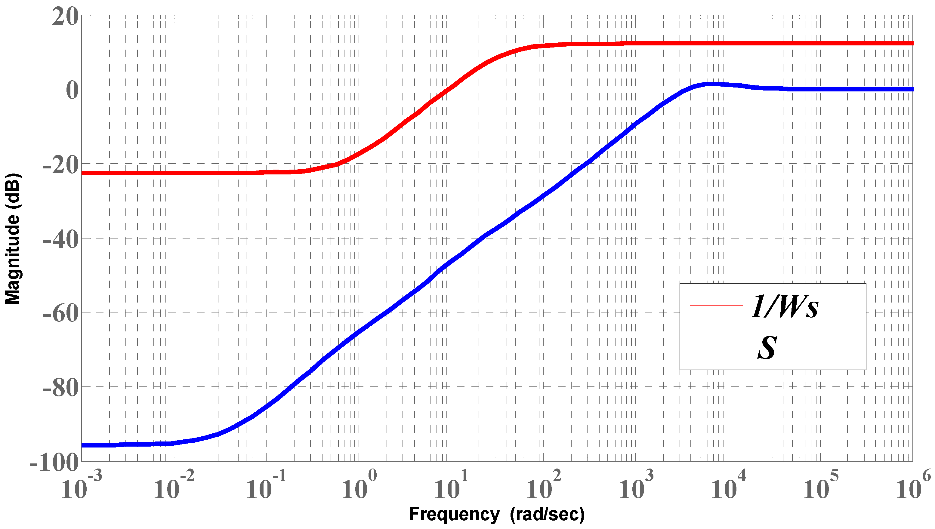
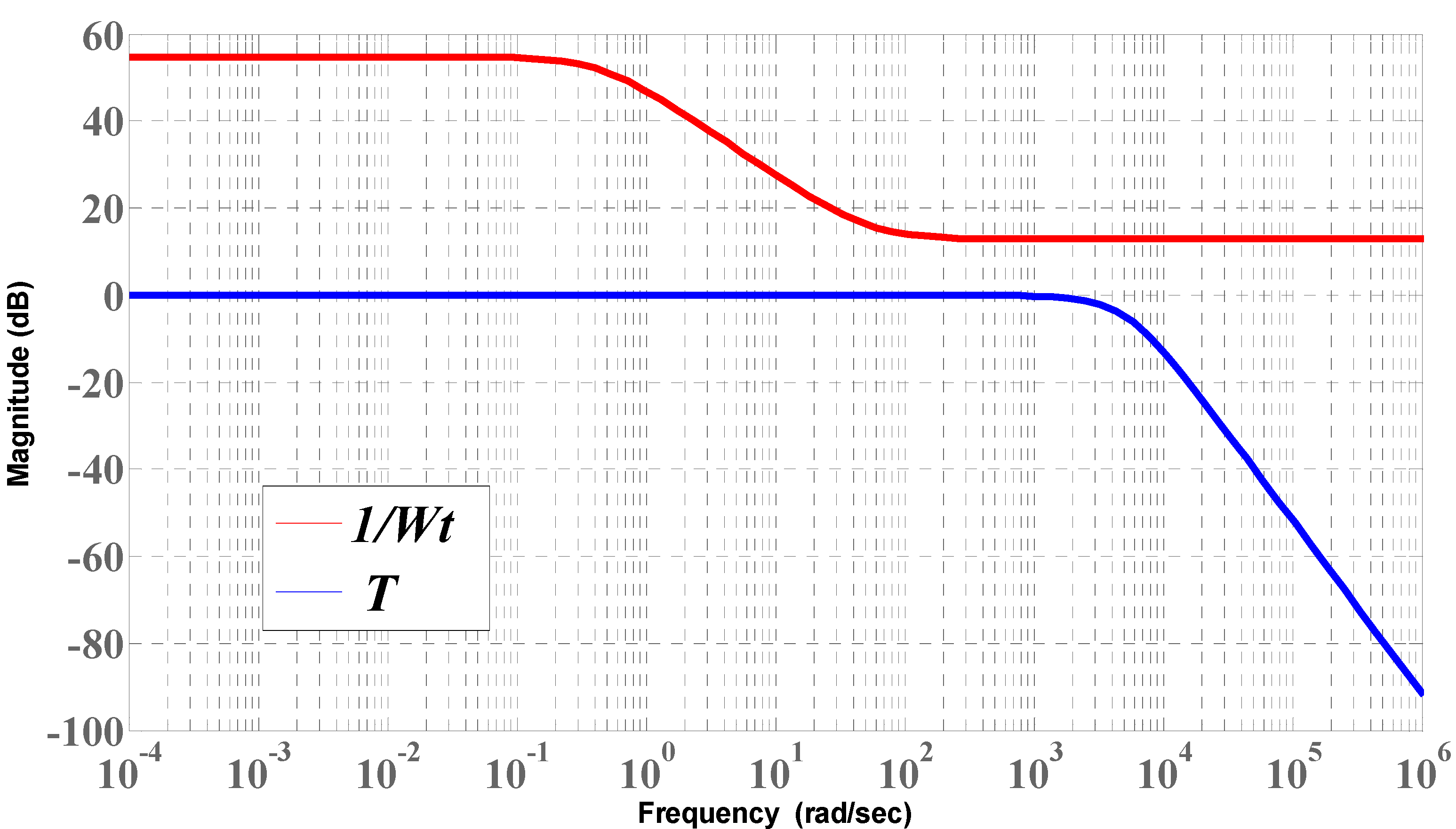
The desirable W_s(s) has low-pass characteristics that ensure the tracking performance and disturbance attenuation. The maximum singular value of the sensitivity function S(s) should be less than the maximum singular value of 1/W_s(s) in all frequency domains:

$$\sigma [S(jw)]<\sigma [W_S^{-1}(jw)]$$

(26)

(2)

The weighting function W_r(s) is proposed to decrease the overshoot in the time responses of the system without significantly decreasing the speed of the response [22].It is usually taken as a diagonal constant matrix to avoid the increase in controller order [28].

(3)

W_t(s) restricts the robust boundary of the system. The maximum singular value of sensitivity function T(s) should be less than the maximum singular value of 1/W_t(s) in all frequency domains:

$$\sigma [T(jw)]<\sigma [W_t^{-1}(jw)]$$

(27)

Moreover, W_s(s) and W_t(s) need to satisfy the following inequality constraint:

$$\sigma [W_S^{-1}(jw)]+\sigma [W_t^{-1}(jw)]\ge 1$$

(28)

It is worth noting that the overly improved tracking performance caused the appearance of a peak in the sensitivity curve [21], implying that the system will have less stability margins. Without loss of generality and increasing the order of the controller, W_s(s) and W_t(s) can be approximated using first-order transfer functions, and W_r(s) can be expressed in scalar form:

$$\{\begin{array}{c}{W}_s=\frac{a_1(s+a_2)}{s+a_3}\\ W_r=b\\ W_t=\frac{d_1(s+d_2)}{s+d_3}\end{array}$$

(29)

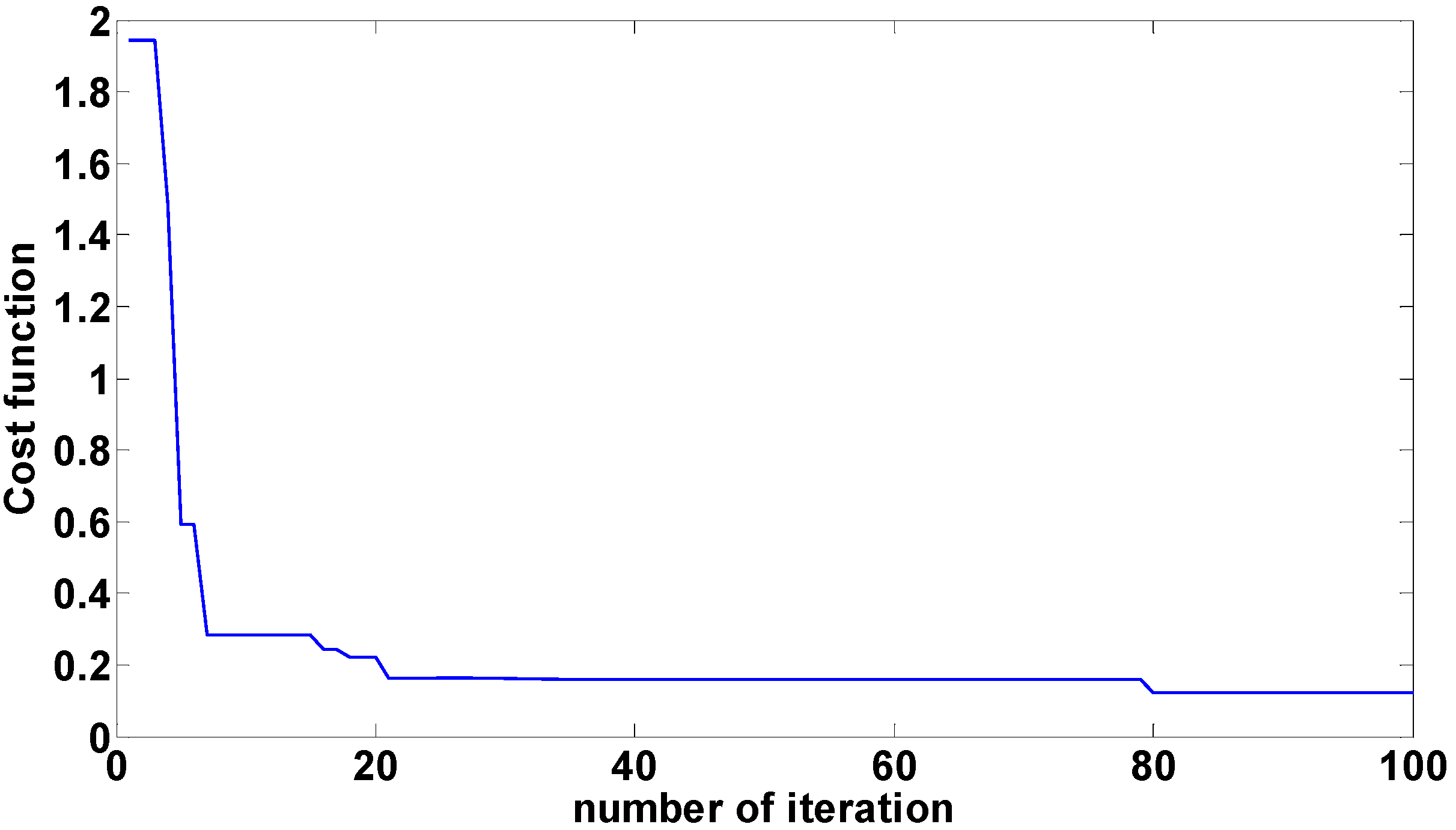
3.3. PSO-Based Controller Design

The PSO algorithm is an evolutionary computation method developed by Kennedy and Eberhart [27,28]. The search performance of the PSO algorithm depends on the balance between global and local exploration abilities. The accurate selection of inertia weights provides a balance between global and local explorations, ω often linearly decreases from 0.9 to 0.4 during a run according to Equation (33).

The impact factors, denoted as ω₁ and ω₂, were introduced into the cost function to achieve the coordination control of the SOFC and SMES as follows:

$$F=\min f(W_S,W_r,W_t)=\min ({\omega }_1{\Vert H_{ZW(SOFC)}\Vert }_{\infty }+{\omega }_2{\Vert H_{ZW(SMES)}\Vert }_{\infty })$$

Subject to:

$$\{\begin{array}{l}\gamma (W_S,W_r,W_t)<1\hfill \\ \begin{array}{l}\sigma [S(jw)]<\sigma [W_S^{-1}(jw)]\\ \sigma [T(jw)]<\sigma [W_t^{-1}(jw)]\end{array}\hfill \\ \sigma [W_S^{-1}(jw)]+\sigma [W_t^{-1}(jw)]\ge 1\hfill \\ a1,a3,b,d1,d2\in (0.0001,1)\hfill \\ a2,d3\in (1,100)\hfill \end{array}$$

(30)

where $\parallel H_{zw\left(SOFC\right)}{\parallel }_{ \infty }$ and $\parallel H_{zw\left(SMES\right)}{\parallel }_{ \infty }$ are the infinity norms of the ratios between the error vector and the disturbance signals.

The population size is 50, and the iteration number is 100. Each particle keeps tracking its coordinates in the problem space:

$$v_{i+1}=w\cdot v_i+c_1\cdot rand\cdot (pbest-x_i)+c_2\cdot rand\cdot (gbest-x_i)$$

(31)

$$x_{i+1}=x_i+v_{i+1}$$

(32)

$$w=w_{\max }-(w_{\max }-w_{\min })\frac{i}{t_{\max }}$$

(33)

The following is the search procedure of the PSO algorithm:

(1)

Specify the parameters of PSO. Initialize the population of the particles with random positions and velocities within the upper and lower bound values.

(2)

Get the generalized plant P(s) of the present parameters and calculate the optimal controllers. Evaluate the cost function for each particle using Equation (30).

(3)

Compare the fitness value of each particle with the pbest and gbest.

(4)

Update the velocity and position of the particle using Equations (31) and (32).

(5)

Check the particle position and velocity and initialize them if they cross the boundaries. Otherwise, increase the iteration by a step.

(6)

When the maximum number of iterations is achieved, stop the process. Otherwise, go to step 2).

The cost function in the optimization problem is optimized using the search procedure. As the number of iterations increase, the cost quickly decreases and finally approximates to the optimal solutions. Figure 5 shows the convergence curve of the cost function. The weighting functions are obtained as follows:

$$\{\begin{array}{c}{W}_s=\frac{0.2438(s+37.16)}{s+0.6771}\\ W_r=0.2457\\ W_t=\frac{0.2263(s+0.4909)}{s+54.54}\end{array}$$

Figure 5. Convergence curve.

Figure 5. Convergence curve.

At the same time, the optimal controllers are obtained as follows:

$$K_{H_2}(s)=\frac{5669.1035(s+61.6)(s+31.28)(s+4.777)(s+1.561)}{(s+8924)(s+71.34)(s+39.18)(s+3.888)(s+2.33)}$$

$$K_M(s)=\frac{948.6821(s+55.82)(s+37.62)(s+4.709)}{(s+8882.5)(s+63.31)(s+38.2)(s+7.249)}$$

$$K_{\alpha }(s)=\frac{3717.7713(s+73.8)(s+32.15)(s+9.2)}{(s+6010)(s+49.18)(s+42.6)(s+2.329)}$$

In Figure 6, the maximum singular value of sensitivity function S(s) is lower than the maximum singular value of 1/W_s(s) in all frequency domains, thus satisfying Equation (26) and guaranteeing the tracking and anti-interference performance.

Figure 6. Singular value curves of sensitivity function S and $W_s^{-1}$.

Figure 6. Singular value curves of sensitivity function S and $W_s^{-1}$.

In Figure 7, 1/W_t(s) covers the T(s) curve completely, according to Equation (27), and hence guarantees the robust stability of the system.

Figure 7. Singular value curves of complementary sensitivity function T and $W_s^{-1}$.

Figure 7. Singular value curves of complementary sensitivity function T and $W_s^{-1}$.

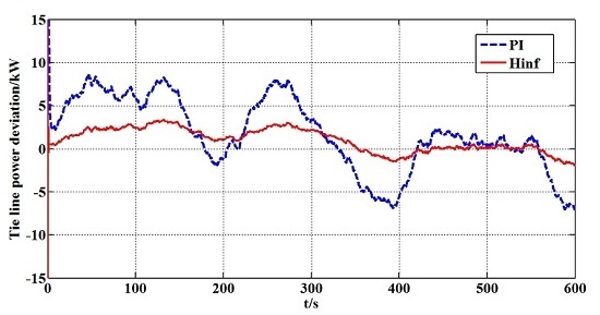
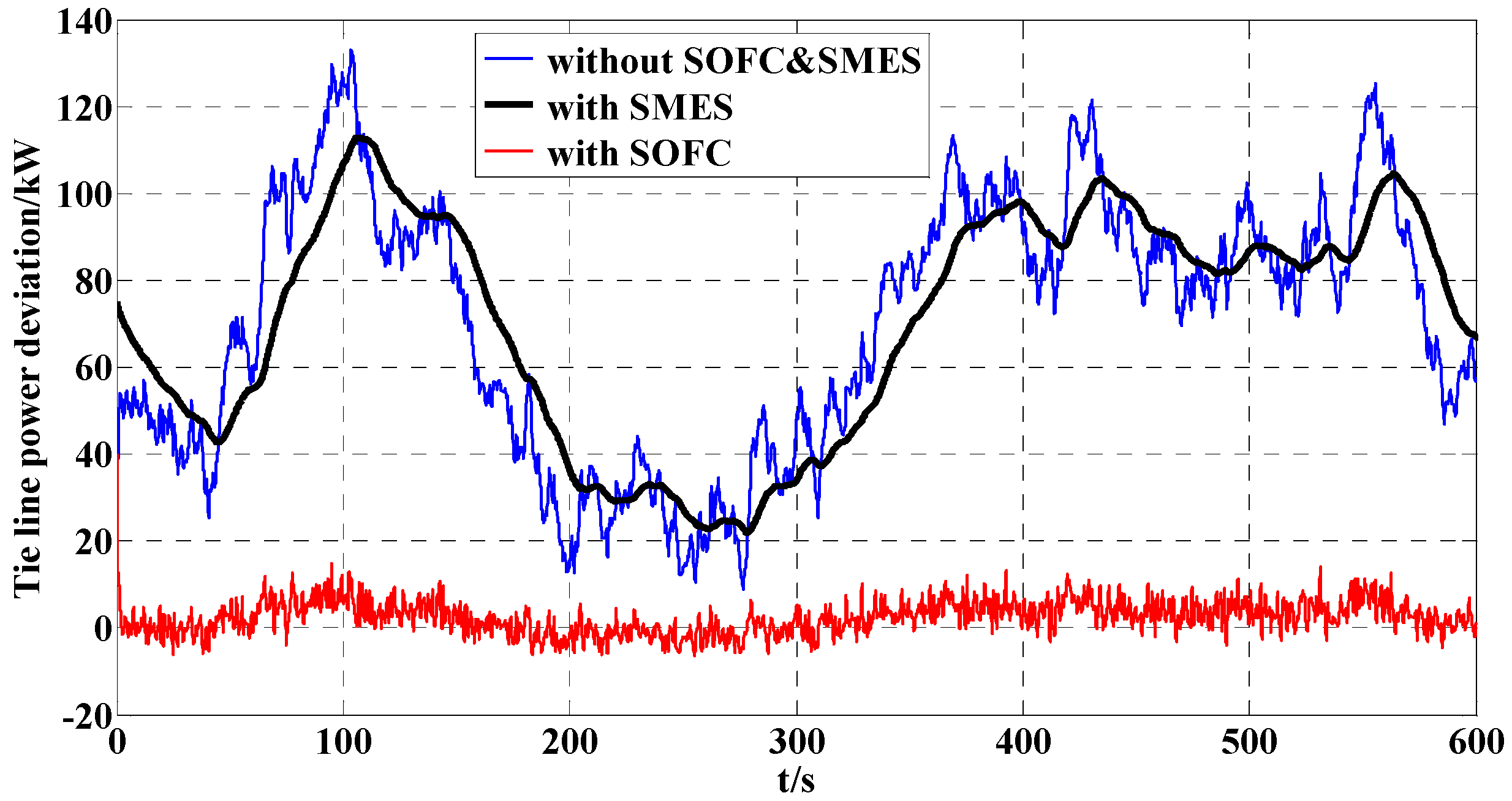
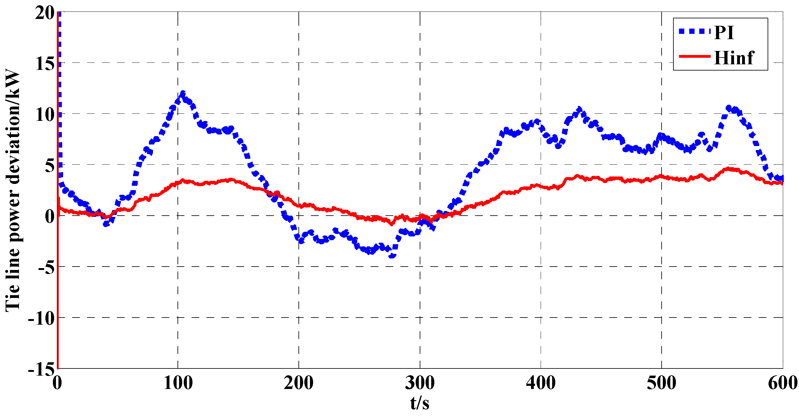
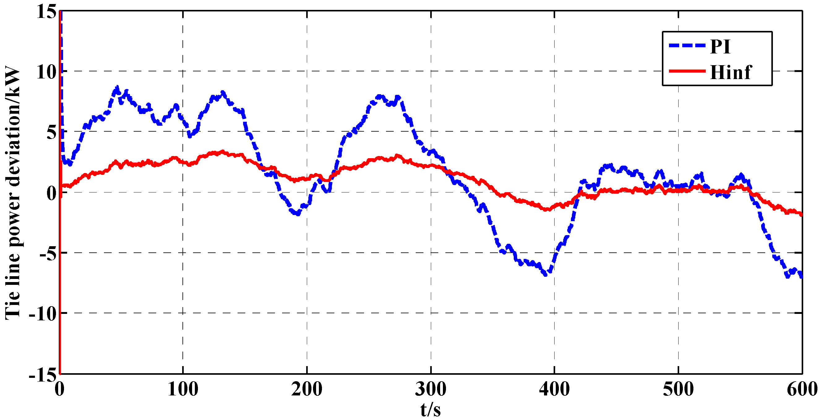
4. Simulation Results

A simulation microgrid is built in MATLAB/Simulink, and the total rated output of DERs is 350 kW, including 200 kW of wind power, 150 kW of SOFC. This paper concentrates on the SOFC dynamic behavior associated with the reactant pressure, neglecting its start-up performance. Thus, its power ranges from 10 kW to 150 kW. The maximum power of the SMES device is set to 50 kW. Random load fluctuates in various conditions. The configuration of the simulated microgrid is connected to the utility grid through a transformer and the SOFC and SMES operate in PQ control mode accurately active power control mode in the interconnected condition. Figure 8 shows the overall control scheme.

Four cases were considered and simulated separately to analyze and compare the performances of the different control strategies and simulation conditions. The comparison is shown in Table 1, where ‘√’ implies that the source is in the microgrid system and ‘×’ implies otherwise.

Table 1. Four cases.

Case	SOFC	SMES	Load conditions
A	√	×	Figure 2
B	×	√	Figure 2
C	√	√	Figure 2
D	√	√	Figure 11

Table 1. Four cases.

Case	SOFC	SMES	Load conditions
A	√	×	Figure 2
B	×	√	Figure 2
C	√	√	Figure 2
D	√	√	Figure 11

In case A, the SOFC was used to meet the needs of tie-line power adjustments. The initial power fluctuations, before the SOFC was installed, were due to the unbalance of wind power and local load. The blue line in Figure 9 shows the real power unbalance using the utility-grid-connected operation before and after installing the SOFC. The real power unbalance can be mitigated to a relatively small range by adjusting the SOFC output as the red line shown in Figure 9. Nevertheless, as discussed in Section I, the SOFC cannot adequately compensate the sudden load changes. Frequent fluctuations can be absorbed by the generator rotor inertia in the utility grid. However, a power quality problem may occur when the microgrid is running in island mode.

Figure 8. Block diagram of the proposed control scheme.

Figure 8. Block diagram of the proposed control scheme.

Figure 9. Tie-line power deviation for case A and case B.

Figure 9. Tie-line power deviation for case A and case B.

In case B, the SMES device was employed into the microgrid. As above-mentioned, the SMES device has fast dynamic response. Wind power fluctuations can be separated into three parts depending on the frequency range. The low-frequency part (0.01 Hz and below) can be compensated using the automatic generation control under grid-connected operation. The objective of the energy storage system compensation can be described as follows:

$$P_{set}=\frac{\tau s}{1+\tau s}\Delta P$$

(34)

where $\frac{\tau s}{1+\tau s}$ is a high-pass filter; τ is a time constant; and τ = 1/2πfc, in which fc is the cut-off frequency (0.01 Hz).

The black line in Figure 9 shows the tie-line power deviation with SMES device. The high-frequency fluctuations were compensated effectively.

In case C, the proposed coordinated SOFC and SMES H∞ controllers were used to satisfy the load demand and smooth the wind power fluctuations simultaneously. Figure 10 shows the tie-line power fluctuations under the PI and proposed control strategies. The PI controllers of SOFC and SMES in the interconnected operation are selected as:

$$\begin{array}{l}{K}_{SOFC}(s)=\mathit{1.0}+\mathit{1.0}/s\\ K_M(s)=1.0+0.8/s\\ K_{\alpha }(s)=0.8+1.0/s\end{array}$$

(35)

Compared with cases A and B, the maximum tie-line power deviation and the smoothing effect of the tie-line power in this case were improved. These results show that the coordinated control enhances the control effect of the microgrid.

Figure 10. Tie-line power curves for case C under PI and proposed control strategies.

Figure 10. Tie-line power curves for case C under PI and proposed control strategies.

In case D, different wind condition and load condition are introduced in simulation to test the validity of the system. New wind power curve and random load curve are shown in Figure 11. Compared with Figure 2, the new load curve decrease in Figure 11 is relatively large since 200 s are required to see how the system responds to this change.

Figure 11. Wind power and random load for case D.

Figure 11. Wind power and random load for case D.

Figure 12 shows the tie-line power curves under the PI and H_infinity control strategies. Obviously the proposed method has better anti-interference performance which is similar to cases C. It is consistent with the actual situation that exchange power supplied from the utility grid decreases along with the load curve decreasing. These results show that the proposed method significantly improves the smoothing effect of wind power fluctuations and confirm the validity of the system in various operating conditions.

Figure 12. Tie-line power curves for case D under PI and proposed control strategies.

Figure 12. Tie-line power curves for case D under PI and proposed control strategies.

5. Conclusions

This paper has presented the application of SOFC and SMES coordinated control in mitigating the impact of wind power fluctuations in a power system. Considering the uncertainties in wind power and load, the robust coordinated controller was designed using the mixed-sensitivity problem of the H∞ control theory and the parameters were obtained by optimizing the weighting functions using the PSO algorithm. The simulation results confirm that the proposed control strategy significantly smoothed the wind power fluctuations. However, the microgrid system established in this paper is limited to wind power and certain storage devices. Thus, more kinds of RESs and different working conditions will be taken into consideration in future studies. Furthermore, the optimal configuration of energy storages will be of interest, both in terms of economic point of view and stability maintenance.

References

- Suvire, G.O.; Mercado, P.E.; Ontiveros, L.J. Comparative Analysis of Energy Storage Technologies to Compensate Wind Power Short-Term Fluctuations. In Proceedings of IEEE/PES Transmission and Distribution Conference and Exposition, Sao Paulo, Brazil, 8–10 November 2010; pp. 522–528.
- Juan, Y. An integrated-controlled AC/DC interface for microscale wind power generation systems. IEEE Trans. Power Electron. 2011, 26, 1377–1384. [Google Scholar]
- Blaabjerg, F.; Chen, Z.; Kjaer, S.B. Power electronics as efficient interface in dispersed power generation systems. IEEE Trans. Power Electron. 2004, 19, 1184–1194. [Google Scholar]
- Kim, H.M.; Lim, Y.; Kinoshita, T. An intelligent multiagent system for autonomous microgrid operation. Energies 2012, 5, 3347–3362. [Google Scholar]
- Kim, H.M.; Kinoshita, T.; Shin, M.C. A Multiagent system for autonomous operation of islanded microgrids based on a power market environment. Energies 2010, 3, 1972–1990. [Google Scholar]
- Vachirasriciriku, S.; Ngamroo, I.; Kaitwanidvilaib, S. Application of electrolyzer system to enhance frequency stabilization effect of microturbine in a microgrid system. Int. J. Hydrog. Energy 2009, 34, 7131–7142. [Google Scholar]
- Li, X.; Song, Y.J.; Han, S.B. Study on Power Quality Control in Multiple Renewable Energy Hybrid Microgrid System. In Proceedings of the 2007 IEEE Power Technology, Lausanne, Switzerland, 1–5 July 2007; pp. 2000–2005.
- Li, X.; Song, Y.J.; Han, S.B. Frequency control in micro-grid power system combined with electrolyzer system and fuzzy pi controller. J. Power Sources 2008, 18, 468–475. [Google Scholar]
- Denver, F.C. Integration of a solid oxide fuel cell into a 10 mw gas turbine power plant. Energies 2010, 3, 754–769. [Google Scholar]
- Padullés, J.; Ault, G.W.; McDonald, J.R. An integrated SOFC plant dynamic model for power systems simulation. J. Power Sources 2000, 86, 495–500. [Google Scholar]
- Torgeir, S.; Alan, F.; Murat, K.; Farshid, Z. Macro level modeling of a tubular solid oxide fuel cell. Sustainability 2010, 2, 3549–3560. [Google Scholar]
- Buckles, W.; Hassenzahl, W.V. Superconducting magnetic energy storage. IEEE Power Eng. Rev. 2000, 20, 16–20. [Google Scholar]
- Saejia, M.; Ngamroo, I. Alleviation of power fluctuation in interconnected power systems with wind farm by SMES with optimal coil size. IEEE Trans. Appl. Supercond. 2012, 22, 571504. [Google Scholar]
- Ali, M.H.; Bin, W.; Dougal, R.A. An overview of SMES applications in power and energy systems. IEEE Trans. Sustain Energy 2010, 1, 38–47. [Google Scholar]
- Imaie, K.; Tsukamoto, O.; Nagai, Y. Control strategies for multiple parallel current-source converters of SMES system. IEEE Trans. Power Electron. 2000, 15, 377–385. [Google Scholar]
- Guan, T.Q.; Mei, S.W.; Lu, Q. Robust control design for power system including superconducting magnetic energy storage devices. Autom. Electr. Power Syst. 2001, 25, 1–6. [Google Scholar]
- Ngamroo, I.; Supriyadi, A.N.C.; Dechanupaprittha, S.; Mitani, Y. Stabilization of Tie-Line Power Oscillations by Robust SMES in Interconnected Power System with Large Wind Farms. In Proceedings of IEEE Transmission and Distribution Conference and Exposition, Seoul, Korea, 26–30 October 2009; pp. 1–4.
- Ngamroo, I. Simultaneous optimization of smes coil size and control parameters for robust power system stabilization. IEEE Trans. Appl. Supercond. 2011, 21, 1358–1361. [Google Scholar]
- Doyle, J.C.; Francis, B.A.; Tannenbaum, A.R. Feedback Control Theory; MacMillan: Toronto, ON, Canada, 1992. [Google Scholar]
- Zhou, K.M.; Doyle, J.C. Essentials of Robust Control. Englewood Cliffs; Prentice-Hall: Englewood Cliffs, NJ, USA, 1998. [Google Scholar]
- Oloomi, H.; Hossein, M. Weight Selection in Mixed Sensitivity Robust Control for Improving the Sinusoidal Tracking Performance. In Proceedings of the 42nd IEEE Conference on Decision and Control, Maui, HI, USA, 9–12 December, 2003; pp. 300–305.
- Ortega, M.G.; Vargas, M.; Castaño, F. Improved design of the weighting matrices for the S/KS/T mixed sensitivity problem—Application to a multivariable thermodynamic system. IEEE Trans. Control Syst. Technol. 2006, 14, 82–90. [Google Scholar]
- Cifdaloz, O.; Rodriguez, A.A. H∞ Mixed-Sensitivity Optimization for Infinite Dimensional Plants Subject to Convex Constraints. In Proceedings of the 46th IEEE Conference on Decision and Control, New Orleans, LA, USA, 12–14 December 2007; pp. 866–871.
- Corcuera, A.D.; Pujana-Arrese, A.; Ezquerra, J.M.; Segurola, E.; Landaluze, J. H∞ based control for load mitigation in wind turbines. Energies 2012, 5, 938–967. [Google Scholar]
- Shi, Y.H.; Eberhart, R.C. Empirical Study of Particle Swarm Optimization. In Proceedings of the 1999 Congress on Evolutionary Computation, Washington, DC, USA, 6–9 July 1999; pp. 1945–1950.
- Duan, P.; Xie, K.G.; Gao, T.T.; Huang, X.G. Short-term load forecasting for electric power systems using the PSO-SVR and FCM clustering techniques. Energies 2011, 4, 173–184. [Google Scholar]
- Kennedy, J.; Eberhart, R.C. Particle Swarm Optimization. In Proceedings of IEEE Internet Conference on Neural Networks, Perth, Australia, 27 November–1 December 1995; pp. 1942–1948.
- Gaing, Z.L. A particle swarm optimization approach for optimum design of PID controller in AVR system. IEEE Trans. Energy Convers. 2004, 19, 384–391. [Google Scholar]
© 2013 by the authors; licensee MDPI, Basel, Switzerland. This article is an open access article distributed under the terms and conditions of the Creative Commons Attribution license (http://creativecommons.org/licenses/by/3.0/).
Share and Cite
Zhang, N.; Gu, W.; Yu, H.; Liu, W. Application of Coordinated SOFC and SMES Robust Control for Stabilizing Tie-Line Power. Energies 2013, 6, 1902-1917. https://0-doi-org.brum.beds.ac.uk/10.3390/en6041902
Zhang N, Gu W, Yu H, Liu W. Application of Coordinated SOFC and SMES Robust Control for Stabilizing Tie-Line Power. Energies. 2013; 6(4):1902-1917. https://0-doi-org.brum.beds.ac.uk/10.3390/en6041902
Chicago/Turabian StyleZhang, Ning, Wei Gu, Haojun Yu, and Wei Liu. 2013. "Application of Coordinated SOFC and SMES Robust Control for Stabilizing Tie-Line Power" Energies 6, no. 4: 1902-1917. https://0-doi-org.brum.beds.ac.uk/10.3390/en6041902