Design and Implement a Digital H∞ Robust Controller for a MW-Class PMSG-Based Grid-Interactive Wind Energy Conversion System

Abstract

A digital $H_{\infty }$ controller for a permanent magnet synchronous generator (PMSG) based wind energy conversion system (WECS) is presented. Wind energy is an uncertain fluctuating resource which requires a tight control management. So, it is still an exigent task for the control design engineers. The conventional proportional-integral (PI) control is not ideal during high turbulence wind velocities, and the nonlinear behavior of the power converters. These are raising interest towards the robust control concepts. The robust design is to find a controller, for a given system, such that the closed-loop system becomes robust that assurance high-integrity and fault tolerant control system, robust $H_{\infty }$ control theory has befallen a standard design method of choice over the past two decades in industrial control applications. The robust $H_{\infty }$ control theory is also gaining eminence in the WECS. Due to the implementation complexity for the continuous $H_{\infty }$ controller, and availability of the high speedy micro-controllers, the design of a sample-data or a digital $H_{\infty }$ controller is very important for the realistic implementation. But there isn’t a single research to evaluate the performance of the digital $H_{\infty }$ controller for the WECS. In this paper, the proposed digital $H_{\infty }$ controller schemes comprise for the both generator and grid interactive power converters, and the control performances are compared with the conventional PI controller and the fuzzy controller. Simulation results confirm the efficacy of the proposed method which are ensured the WECS stabilities, mitigate shaft stress, and improving the DC-link voltage and output power qualities.

1. Introduction

Over the period 1990–2010, fossil fuels (e.g., oil, coal, gas) contributed 83% of the growth in energy. Due to the crisis of exhausting fossil fuels and considering the green-house effect, it is predicted that over the next twenty years, fossil fuels contribute 64% of the growth in energy. Renewables (e.g., wind, solar, hydro, wave, biofuels) account for 18% of the growth in energy to 2030. The rate at which renewables penetrate the global energy market is similar to the emergence of nuclear power in the 1970s and 1980s [1]. 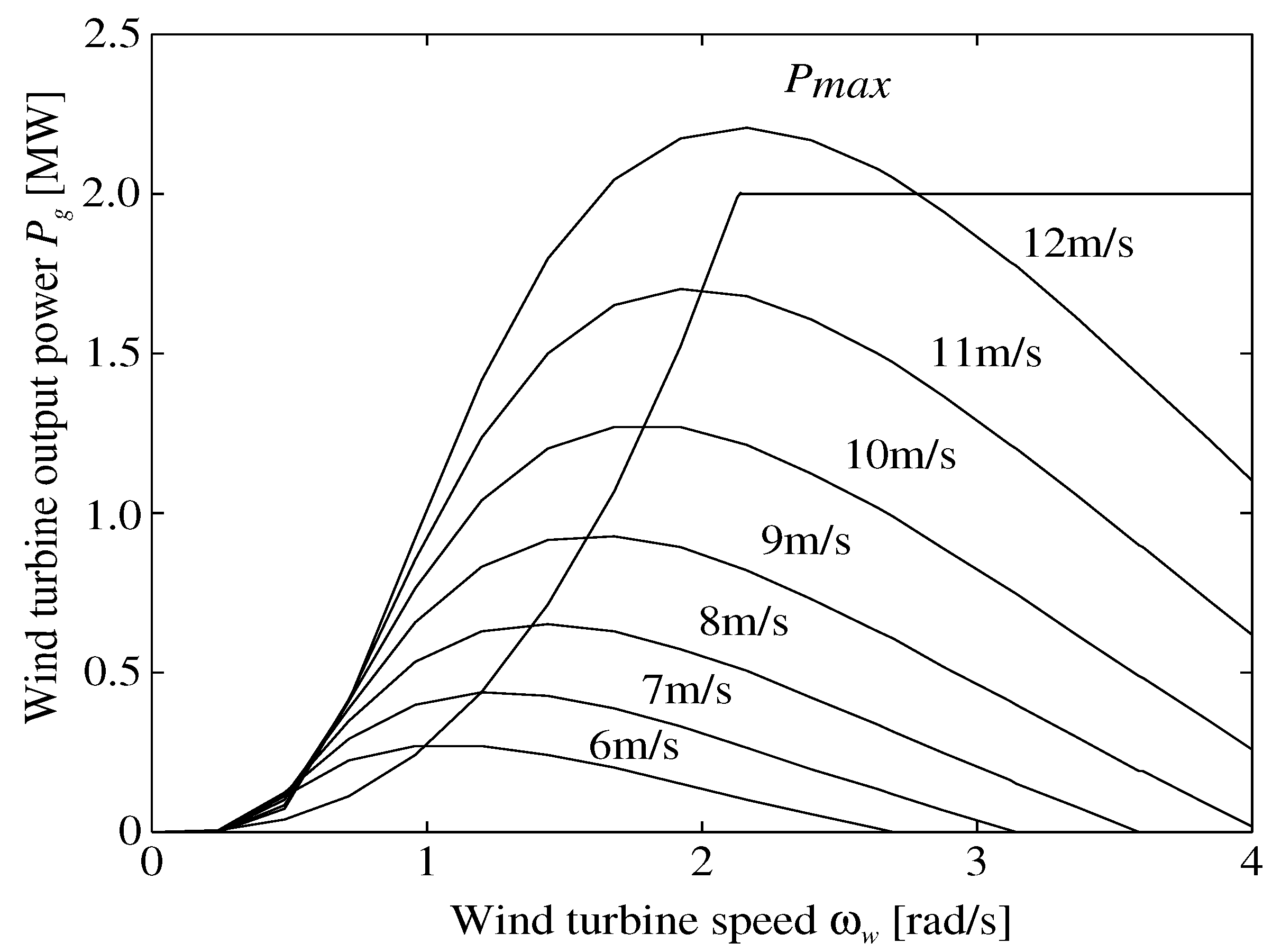Among the renewable sources, wind energy is one of the most rapidly growing renewable power source [2]. Wherever the wind speed exceeds approximately 6 m/s there are possibilities for exploiting it economically, depending on the costs of competing power sources [3].

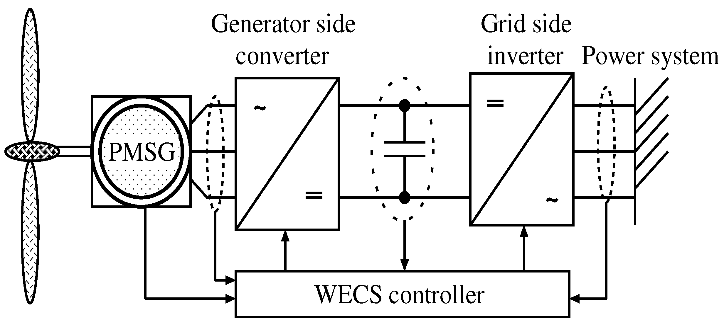
Variable speed wind turbines (VSWTs) can utilize the wind energy proficiently. VSWTs are equipped with the doubly fed induction generators (DFIGs) or the permanent magnet synchronous generators (PMSGs). The popularity of the PMSG based wind energy conversion system (WECS) has been increased because of the simple structure, availability, and efficient power producing capability [4]. However, wind velocity is a highly stochastic component which can diverge very quickly. So, the control of the WECS at different places with different wind velocities is a very challenging task. Various control synthesis methods have been applied in response to the WECS control problems, such as PI control [4,5,6,7,8,9], LQG control [10,11], or fuzzy control [12,13]. Most of the researches [4,5,6,7,8,9,10,11,12,13], provided controllers are designed around an operating point and are valid only for a particular range of operation which are not covered the whole operating region. Most of the cases, wind velocities are chosen within variations ±1 m/s or ±2 m/s of the rated wind velocity, or below the rated wind velocity, and simulation results are provided within single range of wind velocities. Therefore, closed-loop stabilities are guaranteed only for the small-range of parameters deviation. Moreover, these control methods are not robust. During the high wind turbulence, PI controller is not ideal. The adaptive controllers such as fuzzy and LQG, the parameters adjustment of these controllers are computationally expensive [3]. Therefore, taking into account of the power producing capacity of the modern WECS (2–5 MW), the high turbulence wind velocities, and the parameter uncertainties, the researchers have prompted to interest in the robust control concepts (e.g., $H_2$ or $H_{\infty }$ controllers). In particular, the robust $H_{\infty }$ controller formulation for the WECS is adopted in [3,14,15,16,17], to improve the performance at the high turbulence wind velocities, or parameter uncertainties.

In [3,14,15], the $H_{\infty }$ control systems design for the DFIGs. The control performance evaluates in a few parameters within the rated wind speed and some short variations of the rated wind speed. There aren’t comparisons with other conventional methods. In [16,17], the $H_{\infty }$ control system design for the drive-train of the WECS and there are simulation analyses only for the wind speed and rotational speed of the generator. There aren’t descriptions about the generated power and other WECS parameters. On the other hand, continuous signals based $H_{\infty }$ controllers (i.e., continuous $H_{\infty }$ controllers) are designed in all the previous researches. Usually, a $H_{\infty }$ control theory is very complex to design for a particular system. So, it is very complicated to implement a continuous $H_{\infty }$ controller in the real-world systems. The digital $H_{\infty }$ controller can be implemented for a system through the micro-controller. Also, a computer software can handle some complex parts of the controller. Nowadays micro-controller is inexpensive, under $5 for many micro-controllers. It can easy to configure and reconfigure through a software. It is highly adaptable, parameters of the program can change with anytime. Digital computers are much less prone to environmental conditions than capacitors, inductors, etc. To consider these factors, it is very important to design a digital $H_{\infty }$ controller based system. But there isn’t research on the digital $H_{\infty }$ controller based WECS.

This paper presents a digital $H_{\infty }$ controller based grid connected WECS. A sub-optimal $H_{\infty }$ discrete-time loop shaping design procedure (DLSDP) is applied in this paper [18]. Described herein is a comprehensive and systematic way of implementing a new methodology of $H_{\infty }$ control design algorithm for a 2 MW PMSG based WECS in a power system. The mechanical dynamics are controlled by PI based pitch angle control system while generator-side converter and grid-side inverter are regulated via the digital $H_{\infty }$ controller. The proposed method is compared with the conventional PI controller method and the fuzzy controller method. Operational stabilities, reduced shaft stress, and improved voltage and power qualities are verified by the MATLAB/SIMULINK^® environment with the Linear Matrix Inequality (LMI) technique.

2. Wind Energy Conversion System

2.1. Configuration of WECS

Figure 1 shows the interconnection of a PMSG based WECS. Wind energy acquired from the wind turbine is sent to the PMSG. To generate maximum power, rotational speed of the PMSG is controlled by a pulse width modulation (PWM) converter. The output power of the PMSG is supplied to the grid through a generator-side converter and a grid-side inverter.

Figure 1. Wind energy conversion system (WECS) configuration.

Figure 1. Wind energy conversion system (WECS) configuration.

2.2. Dynamic Model of WECS

The maximum input power of the WECS can be expressed as

$$P_{wind}=\frac{1}{2}\rho \pi R_o^2{V}_w^3$$

(1)

where $R_o$ is the wind turbine blade radius; $V_w$ is the wind speed; and ρ is the air density. The wind turbine input torque $T_{wind}$ can be described as

$$\begin{array}{ccc}\hfill T_{wind}& =& \frac{\lambda }{{\omega }_w}{P}_{wind}\hfill \\ \mathrm{(2)}& & =& \frac{1}{2}\rho \pi R_o^3{V}_w^2\hfill \end{array}$$

where ${\omega }_w$ is the rotational speed of the wind turbine; and λ is the tip speed ratio, can be defined as $\lambda =\frac{R_o{\omega }_w}{V_w}$.

The wind turbine output power $P_w$ and the wind turbine output torque $T_w$ (i.e., input torque to the PMSG) are defined by the following equations:

$$\begin{array}{c}\hfill P_w=\frac{1}{2}{C}_p(\lambda ,\beta )\rho \pi R_o^2{V}_w^3\end{array}$$

(3)

$$\begin{array}{c}\hfill T_w=\frac{1}{2}{C}_p(\lambda ,\beta )\rho \pi R_o^3{V}_w^2/\lambda \end{array}$$

(4)

where $C_p$ is the power coefficient; and β is the pitch angle. The power coefficient $C_p$ is defined by the following equation:

$$C_p=0.22(\frac{116}{\Gamma }-0.4\beta -5){exp}^{-\frac{12.5}{\Gamma }}$$

(5)

$$\Gamma =\frac{1}{\frac{1}{\lambda +0.08\beta }-\frac{0.035}{{\beta }^3+1}}$$

(6)

From Equations (3) and (5), the WECS output power characteristics are represented in Figure 2, from which it can be seen that, for a particular wind speed, there is a rotational speed ${\omega }_{opt}$, is known as optimum rotational speed, which generates the maximum power $P_{max}$. In this way, the maximum power point tracking (MPPT) control to each wind speed can increase the power generation for VSWTs. The value of ${\omega }_{opt}$ is calculated by the differentiating $C_p$ with respect to the ${\omega }_w$. Therefore, ${\omega }_{opt}$ is approximated as follows [4]:

$${\omega }_{opt}=0.1874V_w$$

(7)

If ${\omega }_w={\omega }_{opt}$, the maximum output power $P_{max}$ of the wind turbine can be obtained. The MPPT control activates when the wind speed $V_w$ is less than the rated wind speed ($V_{w\_rated}$ = 12 m/s), and above the rated wind speed, the output power of the PMSG is controlled by the pitch angle system. In this paper, the pitch angle is controlled in the region between the cut-in wind speed (5 m/s) and the cut-out wind speed (24 m/s). The pitch angle control system is shown in Figure 3. The pitch angle command ${\beta }_{CMD}$, is determined from the PI controller and the pitch angle selector. The pitch angle β, is constant at $2^{\circ }$ when the power error of the PMSG $\Delta P_g$, is zero. If $\Delta P_g$ is positive, β will increase to reduce the output power to maintain the rated power of the PMSG $P_g$, and vice versa. Above the cut-out wind speed, β is set as ${90}^{\circ }$ for the safety of the WECS. Actually, the pitch angle control system includes a hydraulic servo system that drives the wind turbine blades according to ${\beta }_{CMD}$. The ${\beta }_{CMD}$ is limited through a limiter within $2^{\circ }$∼${90}^{\circ }$ and the maximum rate of change is $\pm {10}^{\circ }$/s.

Figure 2. WECS output power characteristics.

Figure 2. WECS output power characteristics.

Figure 3. Pitch angle control system.

Figure 3. Pitch angle control system.

2.3. Mathematical Model of PMSG

Generally, the mathematical model of a PMSG is same as the permanent magnet synchronous motor (PMSM). The voltage and torque equations of the PMSM in the synchronous reference frame are given by the following equations:

$$\begin{array}{ccc}\hfill v_d& =& R_a{i}_d+L_d\frac{d{i}_d}{dt}-{\omega }_e{L}_q{i}_q\hfill \end{array}$$

(8)

$$\begin{array}{ccc}\hfill v_q& =& {\omega }_e{L}_d{i}_d+R_a{i}_q+L_q\frac{d{i}_q}{dt}+{\omega }_{e}K\hfill \end{array}$$

(9)

$$\begin{array}{ccc}\hfill T_e& =& p\{K{i}_q+(L_d-L_q)i_d{i}_q\}\hfill \end{array}$$

(10)

where $v_d$ and $v_q$ are the $dq$-axis voltages; $i_d$ and $i_q$ are the $dq$-axis currents; $R_a$ is the stator resistance; $L_d$ and $L_q$ are the $dq$-axis inductances; ${\omega }_e$ is the electrical rotational speed; K is the permanent magnetic flux; and p is the number of pole pairs. Power generation starts when the electromagnetic torque $T_e$ is negative. In addition, the motion equations of the PMSG and wind turbine are given by the following equations [19,20]:

$$T_e=J_{eq}\frac{d{\omega }_g}{dt}+D{\omega }_g+T_{lw}$$

(11)

$$T_w=J_w\frac{d{\omega }_w}{dt}+T_{lw}$$

(12)

where D is the rotational damping; $J_{eq}(J_{eq}=J_g+J_w)$ is the equivalent inertia; $T_{lw}$ is the load torque; and ${\omega }_g$ is the mechanical rotational speed.

Figure 4 demonstrates a schematic of the WECS mechanics, presented as a shaft coupling the two parts: turbine or rotor side and generator side. Since the PMSG is direct-driven, the gear box does not include here. The spring constant $K_s$ and the corresponding damping coefficient D are related to the rotor side. The three-step model of drive train is shown in Figure 4 which is expressed in state-space format as follows:

$$\left[\begin{array}{c}\dot{{\theta }_s}\\ \dot{{\omega }_w}\\ \dot{{\omega }_g}\end{array}\right]=\left[\begin{array}{ccc}0& 1& -1\\ -\frac{K_s}{J_w}& -\frac{D}{J_w}& \frac{D}{J_w}\\ \frac{K_s}{J_g}& \frac{D}{J_g}& -\frac{D}{J_g}\end{array}\right]\left[\begin{array}{c}{\theta }_s\\ {\omega }_w\\ {\omega }_g\end{array}\right]+\left[\begin{array}{cc}0& 0\\ \frac{T_w}{J_w}& 0\\ 0& -\frac{T_e}{J_g}\end{array}\right]$$

(13)

where ${\theta }_s$ is the shaft angular twist and it is equivalence to the ${\omega }_w-{\omega }_g$.

Figure 4. Two-mass shaft model of WECS.

Figure 4. Two-mass shaft model of WECS.

Variable-speed operation of the WECS is increased the fluctuation of output power and somewhat raises the shaft fatigue cycles. Drive train dynamics, system losses, and evading resonant frequencies can be integrated using proper control system implementation, by modifying the reference value for the aerodynamic torque near the resonant rotor speed. The proposed digital $H_{\infty }$ control method aspires to the lower fluctuations in shaft torsional torque.

3. Power Converter Control System of WECS

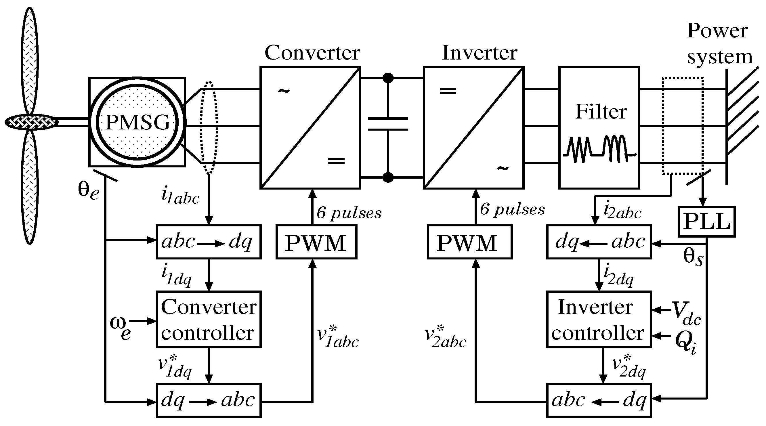
The WECS adopts an AC-DC-AC power converter method with voltage source converters (VSCs). The PMSG is connected to the grid through two PWM VSCs: a generator-side converter and a grid-side inverter. The generator-side converter controls the generator torque of the PMSG, while the grid-side inverter controls the DC-link voltage and the grid voltage, respectively. The power converter control system is shown in Figure 5. Each of the four quadrant power converters is a standard 3-phase two-level unit, composed of six insulated gate bipolar transistors (IGBTs) and controlled by the triangular-wave (10 kHz) PWM law. Each of the configurations of the control system is described below.

Figure 5. Power converter control system.

Figure 5. Power converter control system.

3.1. Conventional PI Control System

3.1.1. Generator-Side Converter

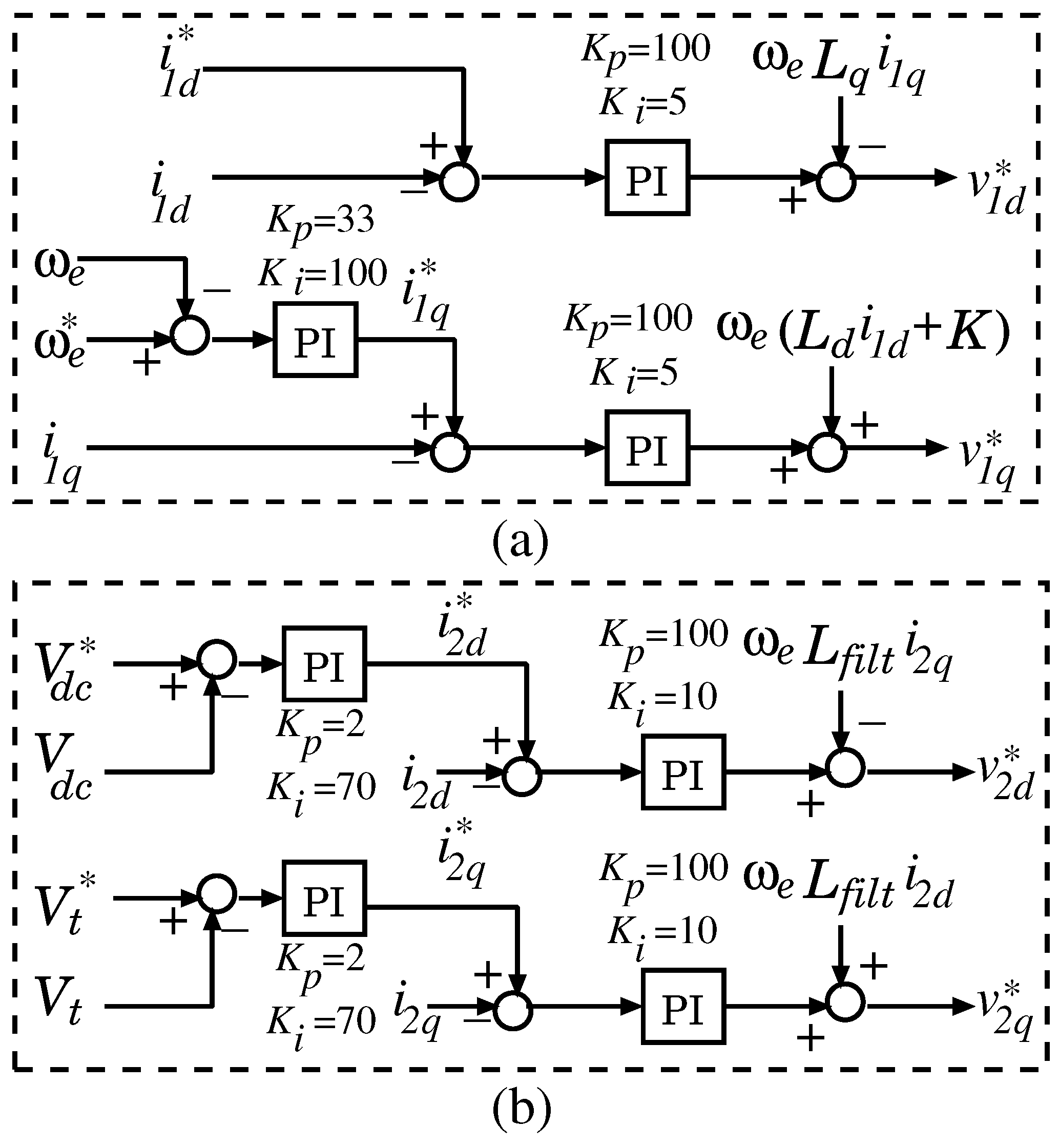
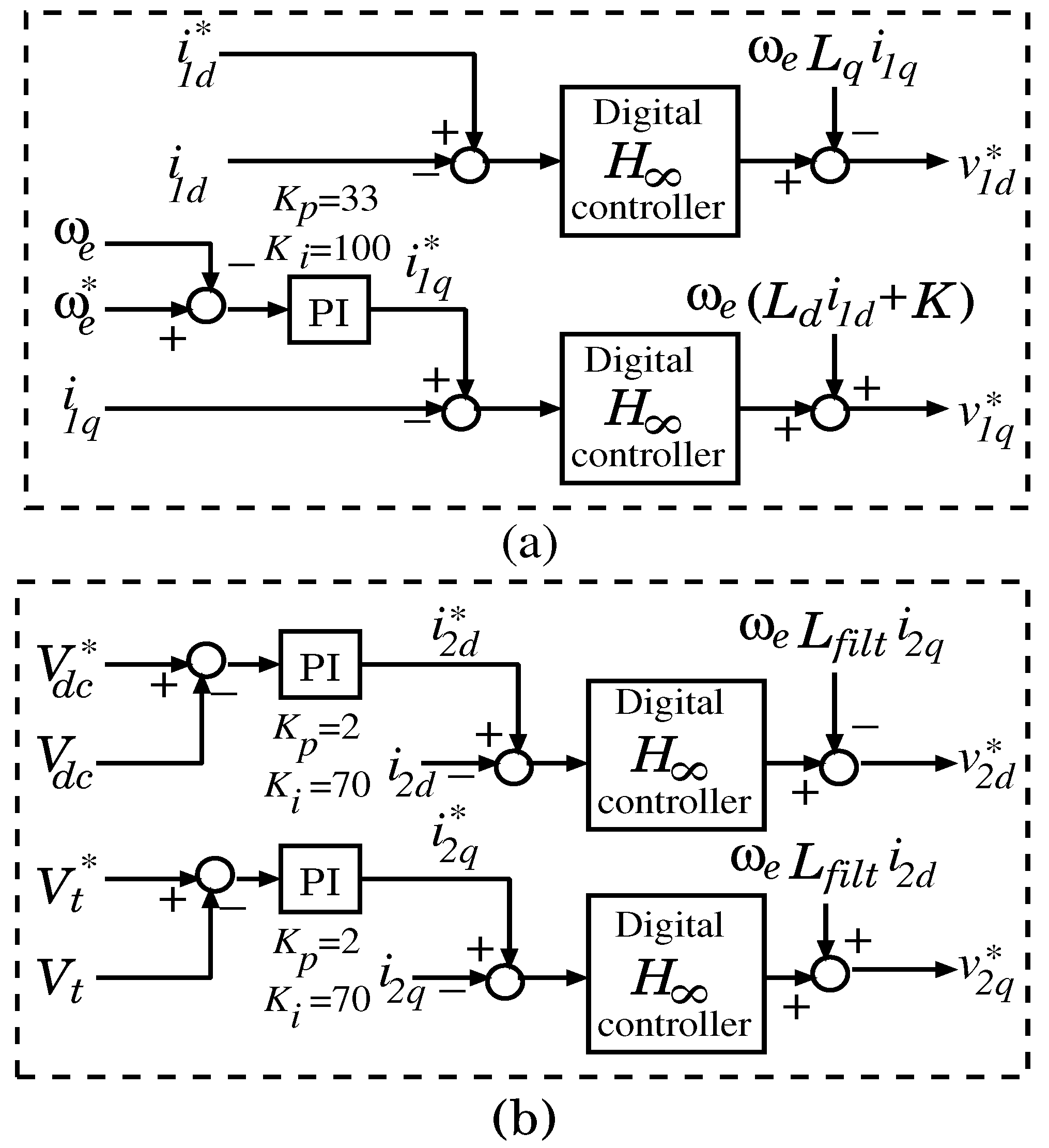
The generator-side converter controls the rotational speed of the PMSG. The vector control scheme is shown in Figure 6a,b. Output of the speed controller is generated the q-axis stator current command $i_{1q}^{*}$. The d-axis stator current $i_{1d}$, is set to zero. The current controller outputs generate the $dq$-axis voltage commands $v_{1d}^{*}$ and $v_{1q}^{*}$ after decoupling. In this figure, ${\omega }_e$ is the PMSG’s electrical speed, $L_d$ and $L_q$ are the $dq$-axis inductances, and K is the permanent magnet flux.

3.1.2. Grid-Side Inverter

The grid-side inverter controls the DC-link voltage $V_{dc}$ and the grid voltage $V_t$. The DC-link capacitor value is chosen to be 15,000 µF. The control system for the grid-side inverter is shown in Figure 6a. The d-axis current can control the DC-link voltage $V_{dc}$, and the q-axis current can control the grid voltage $V_t$. The $V_{dc}^{*}$ and $V_t^{*}$ are the DC-link voltage command and the grid voltage command, respectively. The controller outputs are $dq$-axis voltage commands $v_{2d}^{*}$ and $v_{2q}^{*}$. The angle ${\theta }_s$ is detected by the phase-locked loop (PLL) for the Park transformation.

The PI controllers gains are shown in each figure. Usually PI controller tuning is a difficult problem due to the limitations of PI controller. The PI controller gains are adjusted by the manual methods for loop tuning.

Figure 6. (a) Generator-side converter control system; (b) Grid-side inverter control system.

Figure 6. (a) Generator-side converter control system; (b) Grid-side inverter control system.

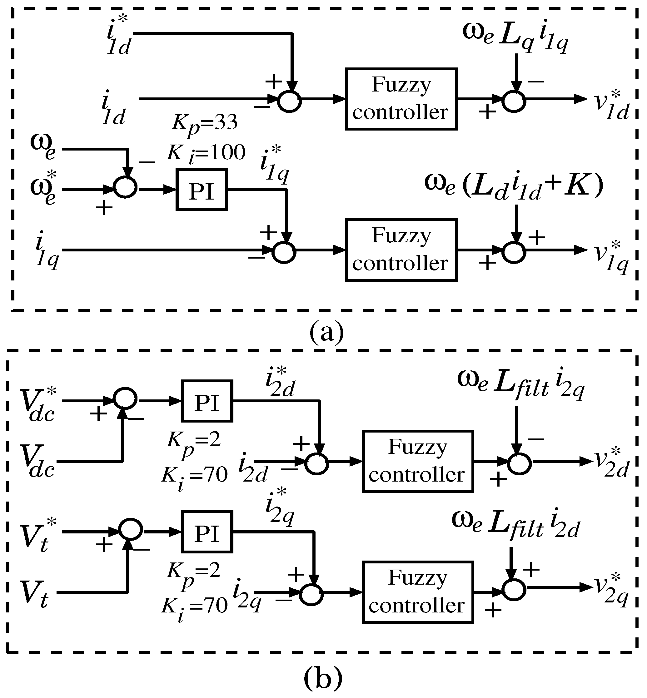
3.2. Fuzzy Control System

Due to the non-linear behavior of the power system and the linearization problems, the control of the variable speed WECS is difficult by using the conventional PI controller methods. The fuzzy controller is a rule based non-linear control technique. The fuzzy controller presents some advantages as compared with the PI controller. It can obtain variable gains depending on the errors and overcomes the problems which are affected by an uncertain model. The detail analyses of the inverter and converter control systems for the WECS are given in previous section. The fuzzy controller based converter control system and inverter control system are shown in Figure 7a,b respectively. From these figures, the conventional PI controllers are replaced by the fuzzy controllers. 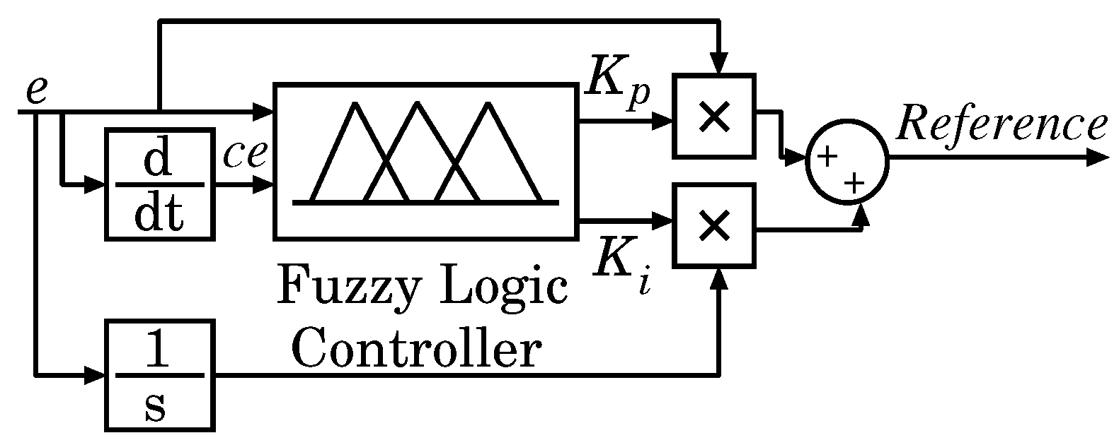Figure 8 shows the detail of the fuzzy based PI control system. It is a multi input−multi output (MIMO) based fuzzy control system. There are two inputs of fuzzy controller such as the system error, e and the change of error $ce$ and two outputs of fuzzy controller that are the proportional gain $K_p$ and the integral gain $K_i$. Depend on error and the change of error, the fuzzy controller delivers the proportional gain $K_p$ and the integral gain $K_i$ for the PI controller, and generates a reference signal. 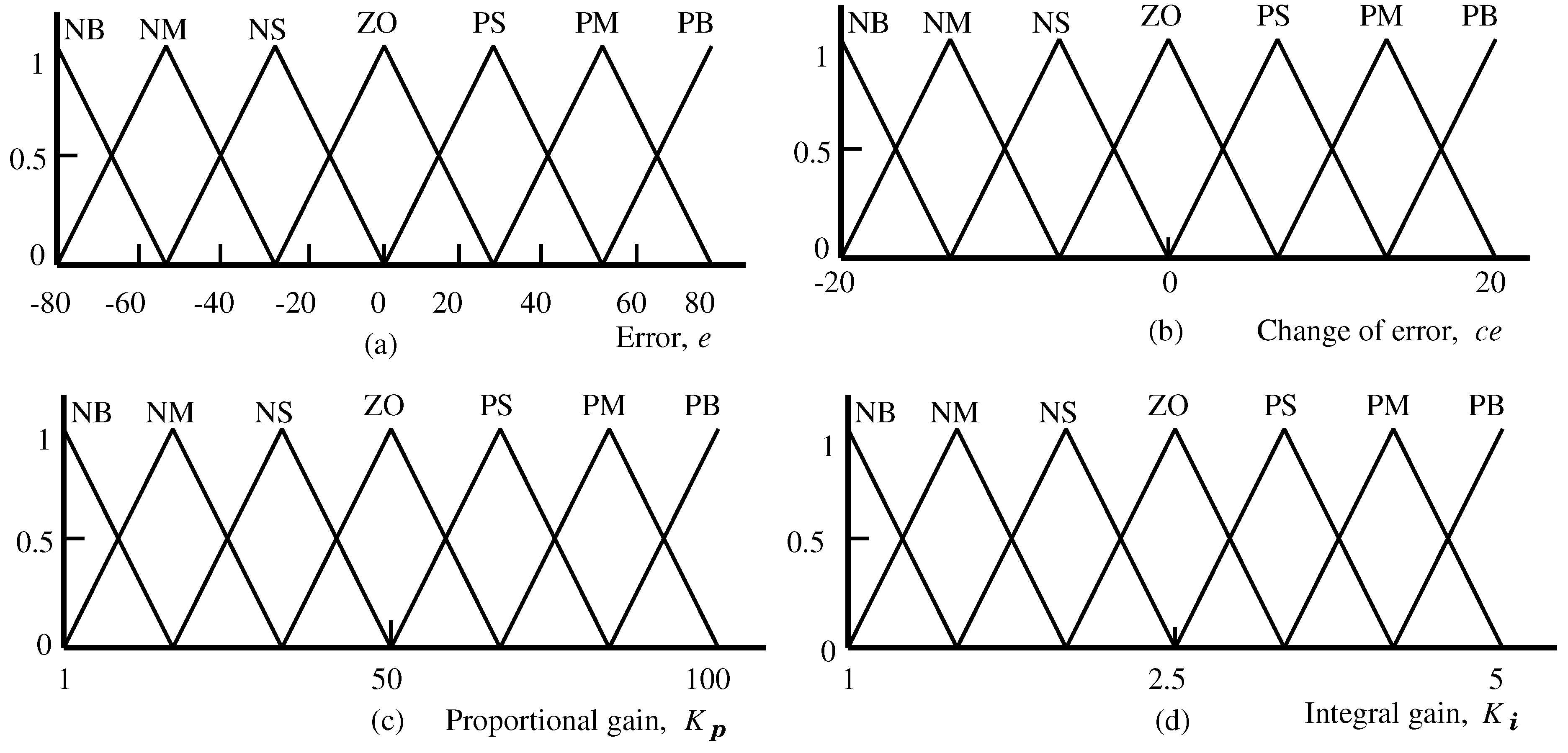Figure 9a,b shows the fuzzy input membership functions (i.e., error and change of error), and Figure 9c,d shows the output membership functions (i.e., proportional gain $K_p$ and integral gain $K_i$) of the fuzzy controller. The fuzzy controller rules are given in Table 1 in which the linguistic variables are represented by negative big (NB); negative medium (NM); negative small (NS); zero (ZO); positive big (PB); positive medium (PM); and Positive small (PS).

Figure 7. (a) Generator-side converter control system; (b) Grid-side inverter control system.

Figure 7. (a) Generator-side converter control system; (b) Grid-side inverter control system.

Figure 8. Fuzzy controller based PI control system.

Figure 8. Fuzzy controller based PI control system.

Figure 9. Fuzzy membership functions (a) input members; error e (b) input members; change of error $ce$ (c) output members; proportional gain $K_p$ (d) output members, integral gain $K_i$.

Figure 9. Fuzzy membership functions (a) input members; error e (b) input members; change of error $ce$ (c) output members; proportional gain $K_p$ (d) output members, integral gain $K_i$.

Table 1. Fuzzy membership functions.

Kp & Ki		e
		NB	NM	NS	ZO	PS	PM	PB
ce	NB	NB	NB	NB	NB	NM	NS	ZO
	NM	NB	NB	NM	NM	NS	ZO	PM
	NS	NB	NM	NS	NM	ZO	PS	PM
	ZO	NB	NM	NS	ZO	PS	PM	PB
	PS	NM	NS	ZO	PS	PS	PM	PB
	PM	NM	ZO	PS	PM	PM	PB	PB
	PB	ZO	PS	PM	PB	PB	PB	PB

Table 1. Fuzzy membership functions.

Kp & Ki		e
		NB	NM	NS	ZO	PS	PM	PB
ce	NB	NB	NB	NB	NB	NM	NS	ZO
	NM	NB	NB	NM	NM	NS	ZO	PM
	NS	NB	NM	NS	NM	ZO	PS	PM
	ZO	NB	NM	NS	ZO	PS	PM	PB
	PS	NM	NS	ZO	PS	PS	PM	PB
	PM	NM	ZO	PS	PM	PM	PB	PB
	PB	ZO	PS	PM	PB	PB	PB	PB

The fuzzy rules and membership functions are determined by the trail-and-error process. Various methods have been proposed for tuning the fuzzy controller, such as selftuning algorithm based on an experimental planning method, where the scaling factors of optimal parameters can be determined efficiently according to the desired performance indexes, Taguchi tuning method, and tuning the membership functions. However, in this paper, the selection of scaling factors is based on the trial-and-error method.

4. Digital $H_{\infty }$ Control Scheme for Power Converters

The implementation of digital control systems and real-time systems belong together. In this section, the proposed digital $H_{\infty }$ robust controller formulation and implementation are described.

4.1. Control Formulation

A generalized digital $H_{\infty }$ robust control problem is shown in Figure 10a, and the feedback configuration is shown in Figure 10b. A stable and detectable n-order of state-space model for the continuous-time plant, P is described by

$$P:\left[\begin{array}{c}\dot{x}\\ z\\ y\end{array}\right]=\left[\begin{array}{ccc}A& B_1& B_2\\ C_1& D_{11}& D_{12}\\ C_2& D_{21}& D_{22}\end{array}\right]\left[\begin{array}{c}x\\ w\\ u\end{array}\right]$$

(14)

$$P:\left\{\begin{array}{c}\dot{x}=Ax+B_{1}w+B_{2}u\hfill \\ z=C_{1}x+D_{11}w+D_{12}u\hfill \\ y=C_{2}x+D_{21}w+D_{22}u\hfill \end{array}\right.$$

(15)

where x ∈ℜ${}^n$ is the state vector; w ∈ℜ${}^{m_1}$ the exogenous input (external input and disturbance) vector; u ∈ℜ${}^{m_2}$ the control input vector; z ∈ℜ${}^{p_1}$ the error (output) vector; and y ∈ℜ${}^{p_2}$ the measurement vector, with $p_1\ge m_2$ and $p_2\le m_1$. The $K\left[z\right]$ is a digital controller to be designed; “s” is the sampler with sampling period τ, i.e., $y_d$ is the input of $K\left[z\right]$ where $y_d\left[k\right]:=y\left(k\tau \right)$. In a real-time process, the average processing time per sample is not greater than the sampling period τ. “H” denotes the generalized hold with hold function $H\left(t\right)$, i.e., u is determined as

$$u\left(t\right)=H\left(t\right)u_d\left[k\right];(k\tau \le t<(k+1)\tau )$$

(16)

where $u_d$ is the output of $K\left[z\right]$. The control goal is to minimize the induced norm of the input-output operator ${\mathcal{T}}_{zw}$:$w\Rightarrow z$. The digital $H_{\infty }$ control problem is solved by searching a digital controller $K\left[z\right]$ and a generalized hold H which internally stabilizes the closed-loop in Figure 10, and the $H_{\infty }$ norm from w to z is smaller than a specified positive number γ, i.e.,

$$\begin{array}{c}\hfill {\parallel {\mathcal{T}}_{zw}\parallel }_{\infty }<\gamma \end{array}$$

(17)

The sub-optimal and DLSDP $H_{\infty }$ controller $K\left[z\right]$ can express as

$$K\left[z\right]:\left[\begin{array}{c}{x}_K[k+1]\\ u_d\left[k\right]\end{array}\right]=\left[\begin{array}{cc}{A}_K& B_K\\ C_K& D_K\end{array}\right]\left[\begin{array}{c}{x}_K\left[k\right]\\ y_d\left[k\right]\end{array}\right]$$

(18)

where

$$\left\{\begin{array}{c}{A}_K={\widehat{A}}_K-{\widehat{B}}_{K}D{(I+{\widehat{D}}_{K}D)}^{-1}{\widehat{C}}_K\hfill \\ B_K={\widehat{B}}_K{(I+D{\widehat{D}}_K)}^{-1}\hfill \\ C_K={(I+{\widehat{D}}_{K}D)}^{-1}{\widehat{C}}_K\hfill \\ D_K={\widehat{D}}_K{(I+D{\widehat{D}}_K)}^{-1}.\hfill \end{array}\right.$$

The estimated values ${\widehat{A}}_K$, ${\widehat{B}}_K$, ${\widehat{C}}_K$, and ${\widehat{D}}_K$ can be obtained to solve the discrete algebraic Riccati equations (DARE) [19].

Figure 10. Digital $H_{\infty }$ control problem (a) Generalized closed-loop configuration; (b) Feedback configuration.

Figure 10. Digital $H_{\infty }$ control problem (a) Generalized closed-loop configuration; (b) Feedback configuration.

The $H_{\infty }$ control problem is adopted by the WECS which is shown in Figure 11. The signal w is represented the reference inputs and some disturbances. The controller output signal u is a control input in the plant. The output z is the control error, ideally it should be zero. The observed output signal y is available for the plant feedback. The detail electrical systems will discuss in the next sub-section.

Figure 11. $H_{\infty }$ control configuration for WECS.

Figure 11. $H_{\infty }$ control configuration for WECS.

4.2. Digital $H_{\infty }$ Control Implementation

The generator-side converter and the grid-side inverter are controlled by the digital $H_{\infty }$ controller which are shown in Figure 12. The configurations of each control system are described in below.

Figure 12. (a) Generator-side converter control method; (b) Grid-side inverter control method.

Figure 12. (a) Generator-side converter control method; (b) Grid-side inverter control method.

4.2.1. Generator-Side Converter

The proposed digital $H_{\infty }$ robust controller converter control system is depicted in Figure 12a. To design a $H_{\infty }$ controller, at first to develop a state-space expression for the generator-side converter. From the Equations (8) and (9), the following equations can be rewritten as:

$$\begin{array}{ccc}\hfill \frac{d}{dt}{i}_{1d}& =& \frac{1}{L_d}\{-R_a{i}_{1d}+{\omega }_e{L}_q{i}_{1q}+v_{1d}\}\hfill \end{array}$$

(19)

$$\begin{array}{ccc}\hfill \frac{d}{dt}{i}_{1q}& =& \frac{1}{L_q}\{-R_a{i}_{1q}-{\omega }_e(L_d{i}_{1d}+K)+v_{1q}\}\hfill \end{array}$$

(20)

From the Equations (19) and (20), the plant state-space expression in (15) can be derived by

$$\begin{array}{ccc}\hfill \left[\begin{array}{c}\dot{i_{1d}}\\ \dot{i_{1q}}\end{array}\right]& =& \left[\begin{array}{cc}-(R_a/L_d)& 0\\ 0& -(R_a/L_q)\end{array}\right]\left[\begin{array}{c}{i}_{1d}\\ i_{1q}\end{array}\right]\hfill \\ \hfill & +& \left[\begin{array}{cccc}0& 0& (1/L_d)& 0\\ 0& 0& 0& -(1/L_q)\end{array}\right]\left[\begin{array}{c}{i}_{1d}^{*}\\ i_{1q}^{*}\\ d_1\\ d_2\end{array}\right]\hfill \\ \mathrm{(21)}& & +& \left[\begin{array}{cc}(1/L_d)& 0\\ 0& (1/L_q)\end{array}\right]\left[\begin{array}{c}{v}_{1d}\\ v_{1q}\end{array}\right]\hfill \end{array}$$

The tracking error z is given as:

$$\begin{array}{ccc}\hfill z& =& \left[\begin{array}{cc}-1& 0\\ 0& -1\end{array}\right]\left[\begin{array}{c}{i}_{1d}\\ i_{1q}\end{array}\right]+\left[\begin{array}{cccc}1& 0& 0& 0\\ 0& 1& 0& 0\end{array}\right]\left[\begin{array}{c}{i}_{1d}^{*}\\ i_{1q}^{*}\\ d_1\\ d_2\end{array}\right]\hfill \\ \mathrm{(22)}& & +& \left[\begin{array}{cc}0& 0\\ 0& 0\end{array}\right]\left[\begin{array}{c}{v}_{1d}\\ v_{1q}\end{array}\right]\hfill \end{array}$$

The measured output y can be written as:

$$\begin{array}{ccc}\hfill y& =& \left[\begin{array}{cc}1& 0\\ 0& 1\end{array}\right]\left[\begin{array}{c}{i}_{1d}\\ i_{1q}\end{array}\right]+\left[\begin{array}{cccc}0& 0& 0& 0\\ 0& 0& 0& 0\end{array}\right]\left[\begin{array}{c}{i}_{1d}^{*}\\ i_{1q}^{*}\\ d_1\\ d_2\end{array}\right]\hfill \\ \mathrm{(23)}& & +& \left[\begin{array}{cc}0& 0\\ 0& 0\end{array}\right]\left[\begin{array}{c}{v}_{1d}\\ v_{1q}\end{array}\right]\hfill \end{array}$$

From the above Equations (21)–(23), state variables x, external inputs and disturbances w, and control inputs u are as:

$$x=\left[\begin{array}{c}{i}_{1d}\\ i_{1q}\end{array}\right],w=\left[\begin{array}{c}{i}_{1d}^{*}\\ i_{1q}^{*}\\ d_1\\ d_2\end{array}\right],u=\left[\begin{array}{c}{v}_{1d}\\ v_{1q}\end{array}\right]$$

(24)

The decoupling components consider as the disturbances to enhance stabilities of the system, as follows

$$\begin{array}{c}\hfill \left\{\begin{array}{c}{d}_1={\omega }_e{L}_q{i}_{1q}\hfill \\ d_2={\omega }_e(L_d{i}_{1d}+K)\hfill \end{array}\right.\end{array}$$

The measured outputs are

$$\begin{array}{c}\hfill y={\left[i_{1d}{i}_{1q}\right]}^T\end{array}$$

(25)

while tracking errors are

$$\begin{array}{c}\hfill z={\left[e_{1id}{e}_{1iq}\right]}^T\end{array}$$

(26)

defined as $e_{1id}=i_{1d}^{*}-i_{1d}$ and $e_{1iq}=i_{1q}^{*}-i_{1q}$.

4.2.2. Grid-Side Inverter

Figure 12b shows the proposed digital $H_{\infty }$ controllers based grid-side inverter control system. The controllers control the DC-bus voltage and the grid-voltage. To develop a state-space expression for the grid-side inverter, the following voltage equations with the $RL$-filter are considered [5].

$$\begin{array}{ccc}\hfill \frac{d{i}_{2d}}{dt}& =& \frac{1}{L_{filt}}\{v_{2d}-R_{filt}{i}_{2d}+{\omega }_e{L}_{filt}{i}_{2q}\}\hfill \end{array}$$

(27)

$$\begin{array}{ccc}\hfill \frac{d{i}_{2q}}{dt}& =& \frac{1}{L_{filt}}\{v_{2q}-R_{filt}{i}_{2q}-{\omega }_e{L}_{filt}{i}_{2d}\}\hfill \end{array}$$

(28)

where $R_{filt}$ is the filter resistance and $L_{filt}$ is the filter inductance. From the above Equations (27) and (28), state-space expression in Equation (15) for the grid-side inverter can be written as:

$$\begin{array}{ccc}\hfill \left[\begin{array}{c}\dot{i_{2d}}\\ \dot{i_{2q}}\end{array}\right]& =& \left[\begin{array}{cc}-(R_{filt}/L_{filt})& 0\\ 0& -(R_{filt}/L_{filt})\end{array}\right]\left[\begin{array}{c}{i}_{2d}\\ i_{2q}\end{array}\right]\hfill \\ \hfill & +& \left[\begin{array}{cccc}0& 0& (1/L_{filt})& 0\\ 0& 0& 0& -(1/L_{filt})\end{array}\right]\left[\begin{array}{c}{i}_{2d}^{*}\\ i_{2q}^{*}\\ d_3\\ d_4\end{array}\right]\hfill \\ \mathrm{(29)}& & +& \left[\begin{array}{cc}(1/L_{filt})& 0\\ 0& (1/L_{filt})\end{array}\right]\left[\begin{array}{c}{v}_{2d}\\ v_{2q}\end{array}\right]\hfill \end{array}$$

The tracking error z can be defined as:

$$\begin{array}{ccc}\hfill z& =& \left[\begin{array}{cc}-1& 0\\ 0& -1\end{array}\right]\left[\begin{array}{c}{i}_{2d}\\ i_{2q}\end{array}\right]+\left[\begin{array}{cccc}1& 0& 0& 0\\ 0& 1& 0& 0\end{array}\right]\left[\begin{array}{c}{i}_{2d}^{*}\\ i_{2q}^{*}\\ d_3\\ d_4\end{array}\right]\hfill \\ \mathrm{(30)}& & +& \left[\begin{array}{cc}0& 0\\ 0& 0\end{array}\right]\left[\begin{array}{c}{v}_{2d}\\ v_{2q}\end{array}\right]\hfill \end{array}$$

The measured output y is defined as:

$$\begin{array}{ccc}\hfill y& =& \left[\begin{array}{cc}1& 0\\ 0& 1\end{array}\right]\left[\begin{array}{c}{i}_{2d}\\ i_{2q}\end{array}\right]+\left[\begin{array}{cccc}0& 0& 0& 0\\ 0& 0& 0& 0\end{array}\right]\left[\begin{array}{c}{i}_{2d}^{*}\\ i_{2q}^{*}\\ d_3\\ d_4\end{array}\right]\hfill \\ \mathrm{(31)}& & +& \left[\begin{array}{cc}0& 0\\ 0& 0\end{array}\right]\left[\begin{array}{c}{v}_{2d}\\ v_{2q}\end{array}\right]\hfill \end{array}$$

From the above Equations (29)–(31), state variables x, the external inputs and disturbances w, and control inputs u are as:

$$\begin{array}{c}\hfill x=\left[\begin{array}{c}{i}_{2d}\\ i_{2q}\end{array}\right],w=\left[\begin{array}{c}{i}_{2d}^{*}\\ i_{2q}^{*}\\ d_3\\ d_4\end{array}\right],u=\left[\begin{array}{c}{v}_{2d}\\ v_{2q}\end{array}\right]\end{array}$$

(32)

The measured outputs are

$$\begin{array}{c}\hfill y={\left[i_{2d}{i}_{2q}\right]}^T\end{array}$$

(33)

The decoupling components are considered as disturbances

$$\begin{array}{c}\hfill \left\{\begin{array}{c}{d}_3={\omega }_e{L}_{filt}{i}_{2q}\hfill \\ d_4={\omega }_e{L}_{filt}{i}_{2d}\hfill \end{array}\right.\end{array}$$

while tracking errors are

$$\begin{array}{c}\hfill z={\left[e_{2id}{e}_{2iq}\right]}^T\end{array}$$

(34)

can be defined as $e_{2id}=i_{2d}^{*}-i_{2id}$ and $e_{2iq}=i_{2iq}^{*}-i_{2iq}$.

The $H_{\infty }$ controller $K\left[z\right]$ supplies the control signal u to the converters to ensure closed-loop stability of the WECS plant P by incorporating feedback. By utilizing a norm reduction method, the $H_{\infty }$ control design problem searches the gain matrix $K\left[z\right]$ such that the $H_{\infty }$-norm conforms to Equation (16) for the closed-loop operator, from the external input variables and disturbances w to the output z. Hence, the $H_{\infty }$ problem is to find the stabilizing controller $K\left[z\right]$ that minimizes Equation (16) and internally stabilizes the closed-loop system subject to the structural constraints dictated by the control law specifications [15].

Numerical analyses of the above values of the proposed digital $H_{\infty }$ controller are verified by the Robust Control Toolbox of the MATLAB^®/SIMULINK.

5. Simulation Results

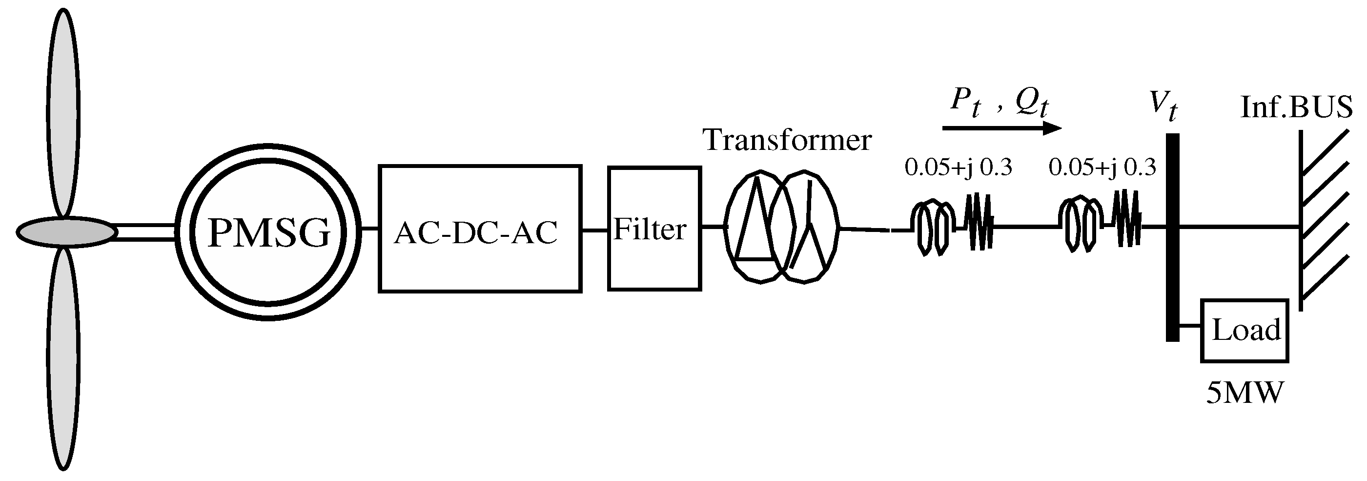
The overall power system for the numerical simulation is shown in Figure 13. In this figure, the grid-side inverter is connected to an infinite bus and a local load through a $RL$-filter, transformer and transmission line. The parameters of the wind turbine, PMSG and power converters are given in APPENDIX. To evaluate effectiveness of the proposed method, WECS operations are verified under two different types of the wind velocities which are confirmed the robust stabilities. The simulation results are compared among the conventional method (i.e., PI controller method), the fuzzy controller method, and the proposed method (i.e., digital $H_{\infty }$ controller method).

Figure 13. Power system model.

Figure 13. Power system model.

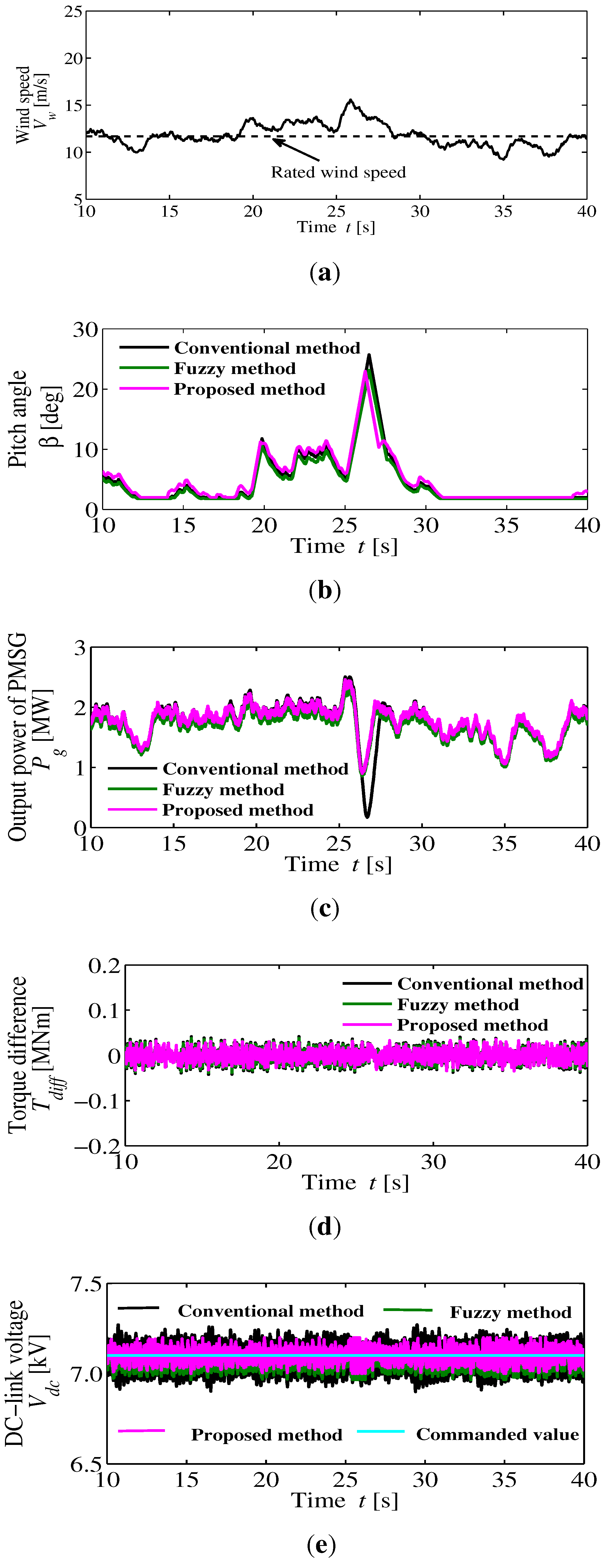
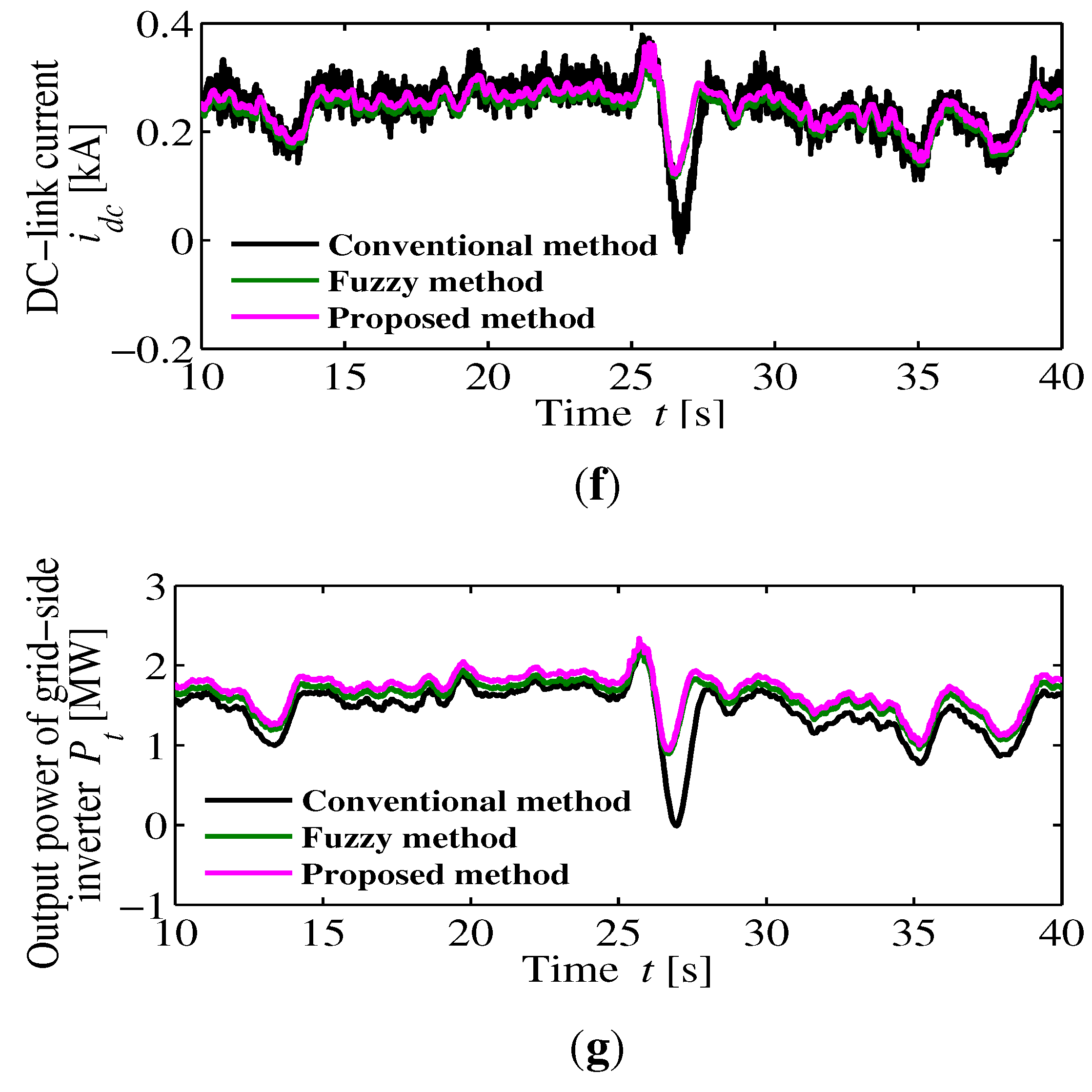
5.1. Low Turbulence Wind Velocity

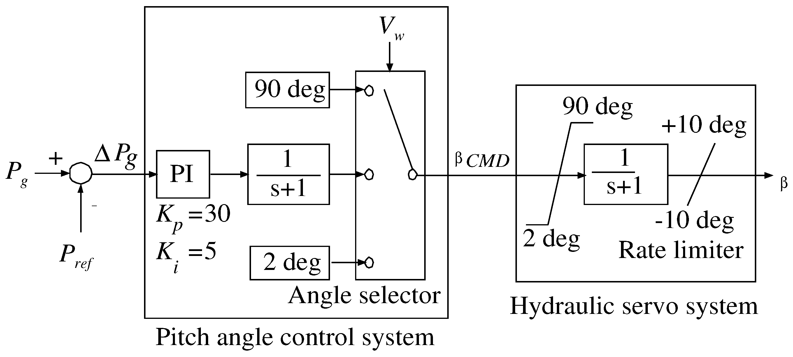
Figure 14 shows the simulation results at the low turbulence wind speed. The wind speed is shown in Figure 14a. The rated wind speed is 12 m/s (dashed line) and wind speed is varied from 9 m/s to 15 m/s. The pitch angle (Figure 14b) activates with respect to the wind speed to control the rated power of the PMSG (2 MW). At simulation time (25–30 s), wind speed is high and the pitch angle is also high in this period. The output power of the PMSG is shown in Figure 14c. From this figure, the proposed method and the fuzzy controller method can generate more stable output power as compared with the conventional PI controller method. At simulation time (25–30 s), output power of the conventional method becomes unstable due to the high fluctuation of wind speed. 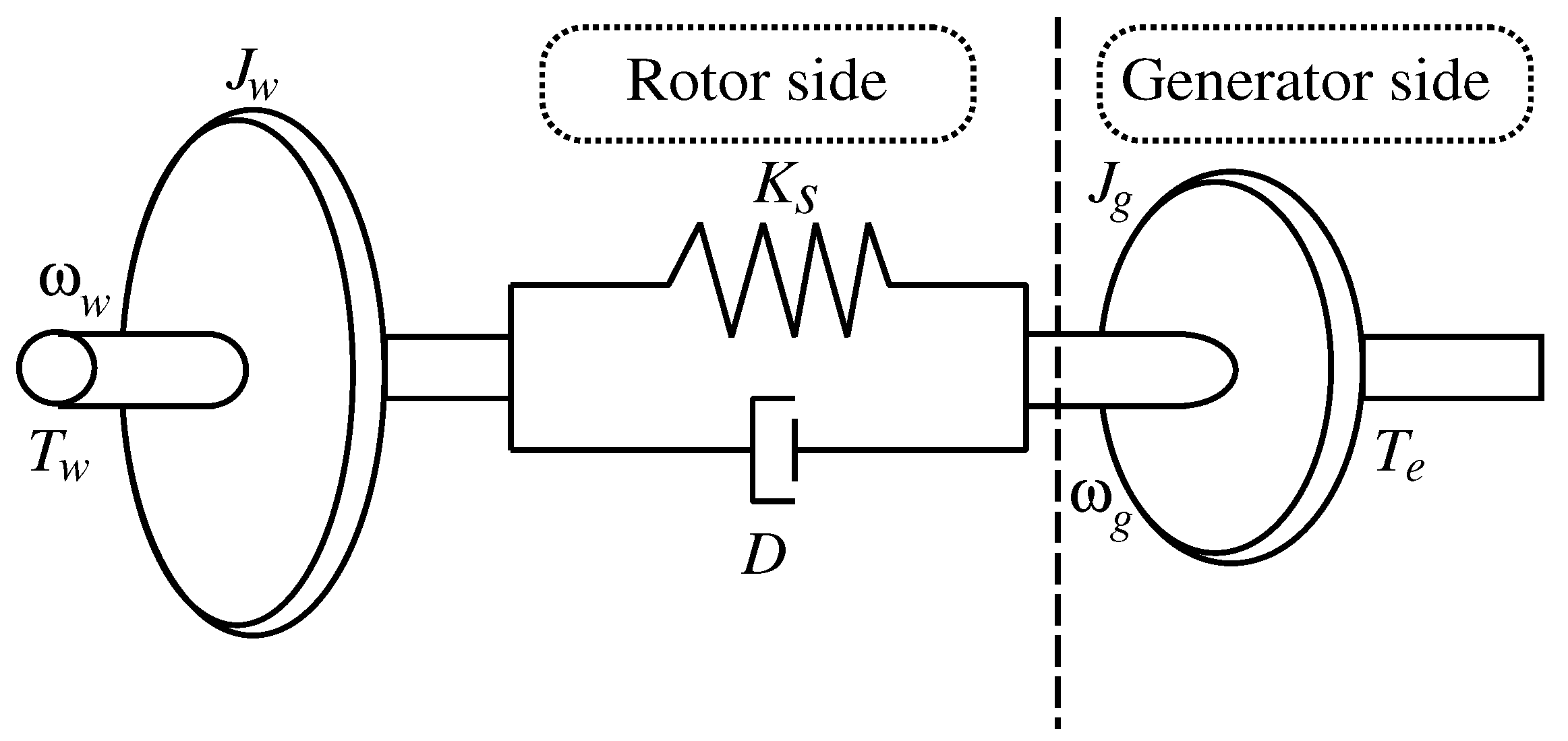In Figure 14d, the torque difference (i.e., difference between input torque and output torque of the PMSG) is reduced by the proposed method as compared with the fuzzy controller method and conventional method. Therefore, the proposed method can reduce the shaft stress of the WECS. From Figure 14e,f, the high frequency components of the DC-link voltage and current are reduced by the proposed method. So, it can reduce the size and stress of the DC-link capacitor. The proposed method can inject an efficient output power to the power grid as compared with the conventional method and the fuzzy controller method which is confirmed in Figure 14g. But the fuzzy controller method can deliver an almost similar power as the proposed method and shows a good performance as compared with the conventional method. From this figure, power loss of the proposed method is lower than that of the conventional method because the proposed method can improve qualities of the torque difference, DC-link current and voltage.

Figure 14. Simulation Results (Low turbulence wind speed). (a) Wind speed; (b) Pitch angle; (c) Output power of PMSG; (d) Torque difference; (e) DC-link voltage; (f) DC-link current; (g) Output power of grid-side inverter.

Figure 14. Simulation Results (Low turbulence wind speed). (a) Wind speed; (b) Pitch angle; (c) Output power of PMSG; (d) Torque difference; (e) DC-link voltage; (f) DC-link current; (g) Output power of grid-side inverter.

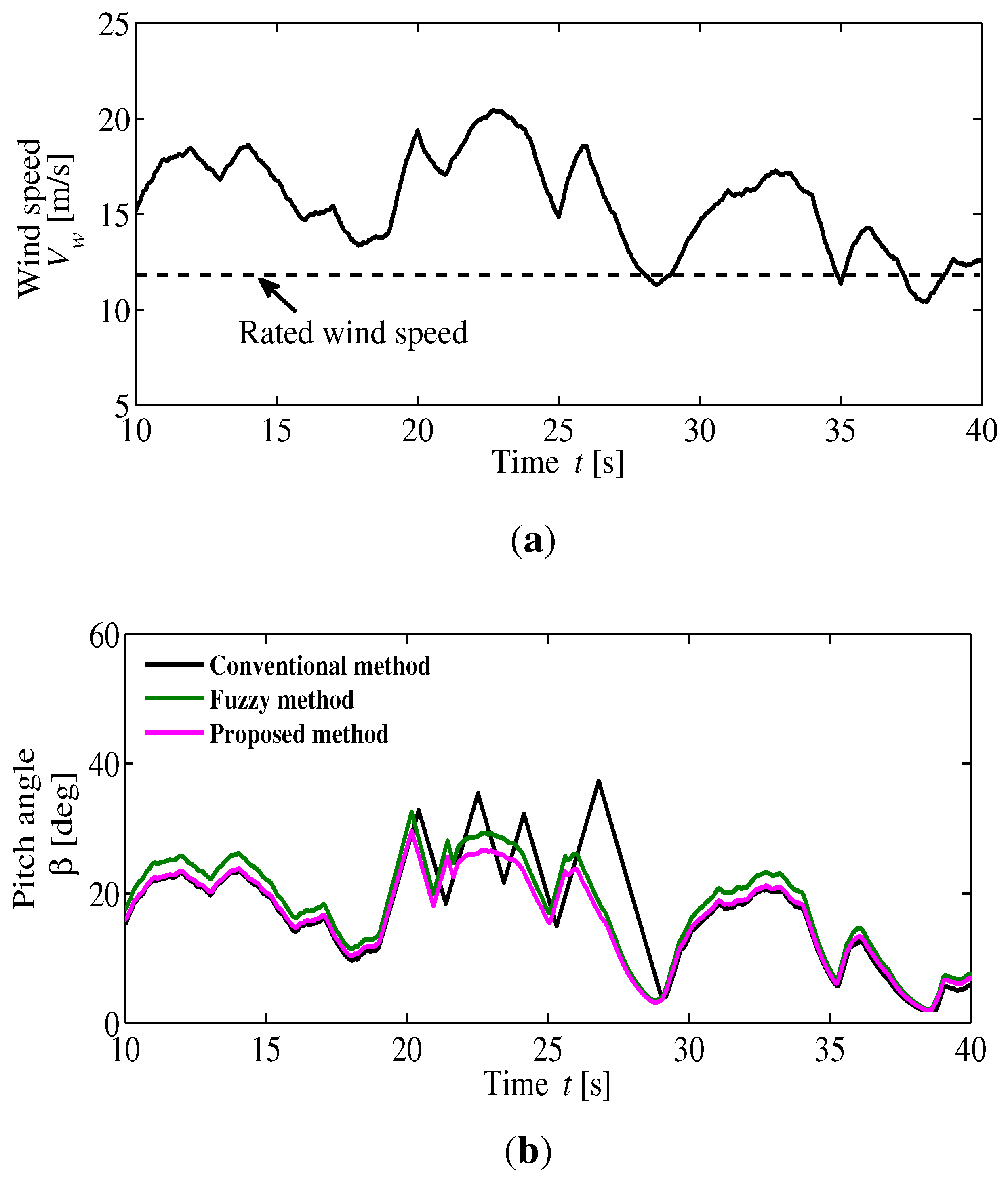
5.2. High Turbulence Wind Velocity

Figure 15 shows the simulation results for another pattern of the wind velocity. It considers as the high turbulence wind speed. The wind speed is received by the WECS which is shown in Figure 15a. It is higher than the rated wind speed. The pitch angle is shown in Figure 15b. Figure 15c,d reflects the final outcomes (i.e., $v_{1q}^{*}$ and $v_{1d}^{*}$) of three different methods. 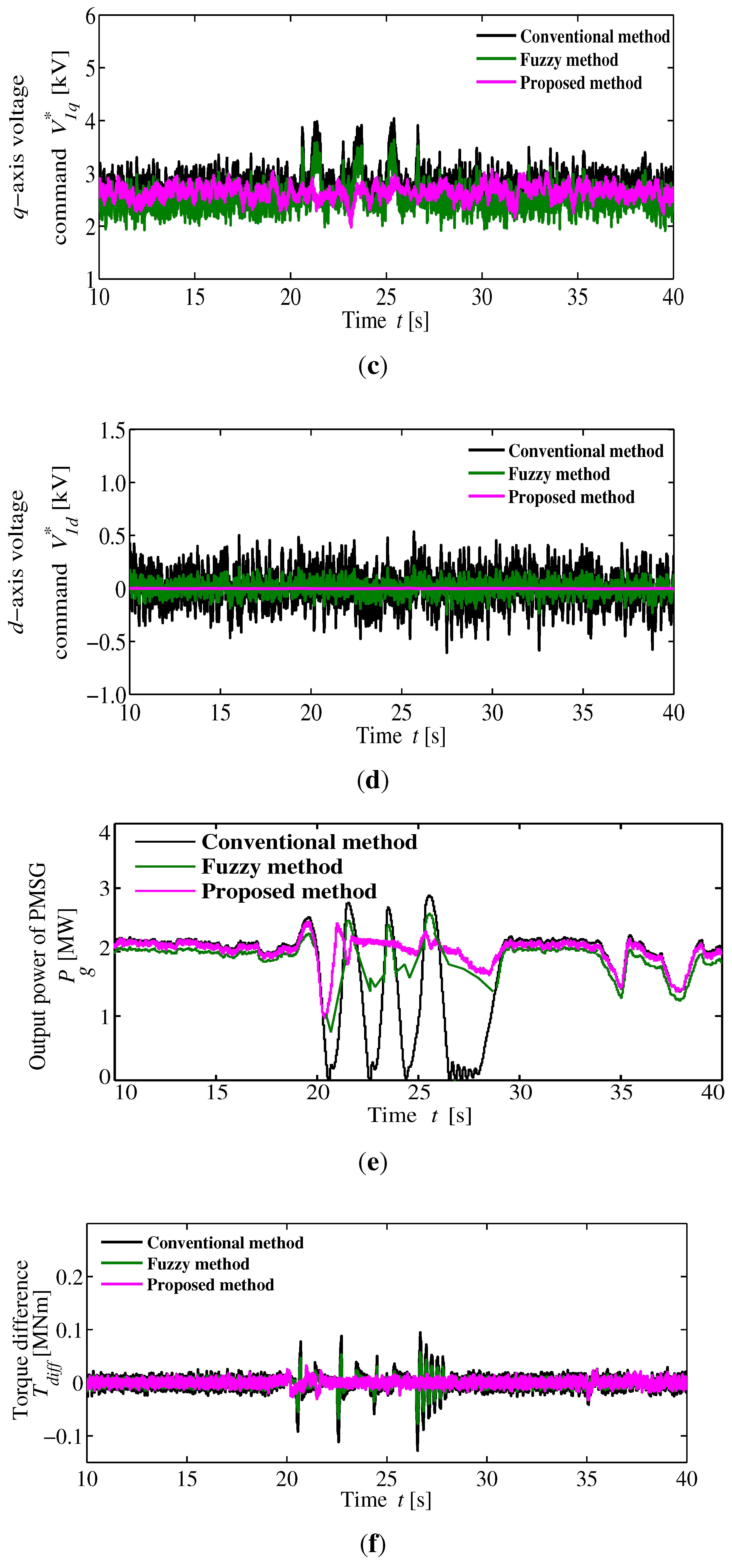In Figure 15c, the q-axis commanded voltage is fluctuated widely by the conventional method and the fuzzy controller method (especially at simulation time 20–30 s) as compared with the proposed method. From Figure 15d, the d-axis commanded voltage is controlled precisely by the proposed method. Usually, the PI controller gains (proportional and integral) adjustment depend on the wind speed. For different set of wind speeds, the PI controller gains are different and required additional adjustments. If the PI controller gains regulate for the low turbulence wind velocities, these may not perfect for the high turbulence wind velocities or vice versa. On the other hand, the fuzzy controller method can show the similar behavior as the proposed in low turbulence wind speed (in Figure 14) but in high turbulence wind velocity the proposed method shows a superior performance as compared with the fuzzy controller method. The tuning of fuzzy controllers (gains and rules) is perfect in the low turbulence wind speed but in high turbulence wind speed, the fuzzy controller requires additional tuning to improve the performance. But in both cases, the fuzzy controller method can improve the performance as compared with the conventional PI controller method. In case of the proposed control method, it can apply at different wind speeds without additional adjustments. Figure 15e shows a comparison of the generated power of the PMSG. From this figure, generated power of the conventional method becomes unstable due to the high turbulence wind velocity. The proposed method can generate stable output power as compared with the conventional method. The fuzzy controller method can generate a stable power as compared with the conventional method but the output power is more fluctuate than the proposed method. In Figure 15f, the torque difference of the PMSG can be reduced significantly by the proposed method as compared with the conventional method and the fuzzy controller method. 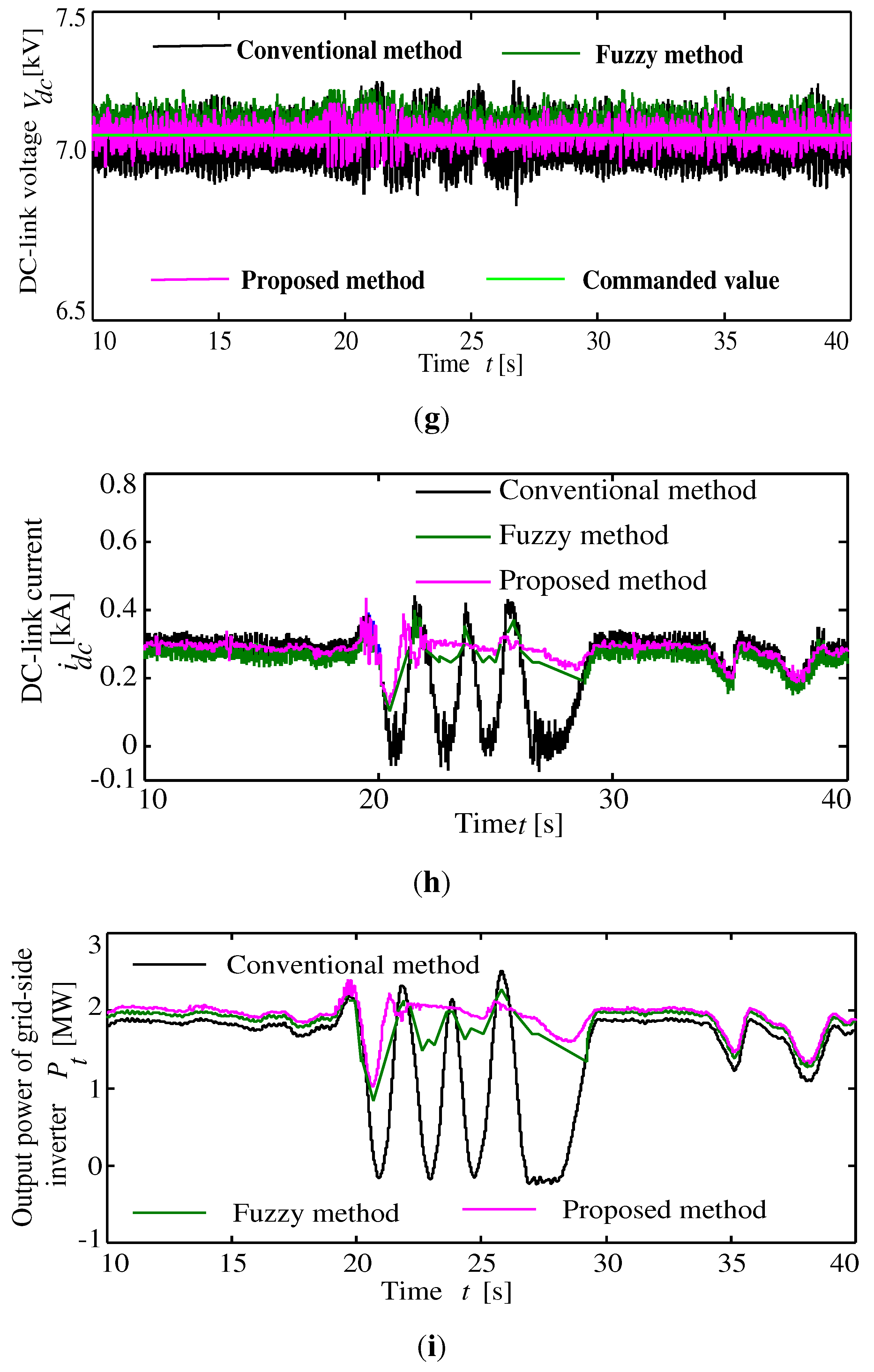The torque difference is much higher than the previous case as shown in Figure 14d. As a result, the proposed method can prevent the shaft stress and the damage of the WECS. High frequency components of the DC-link voltage and current are decreased extensively by the proposed method (Figure 15g,h). So, it can reduce size and stress of the DC-link capacitor. As a consequent, it can increase the life time of the capacitor. The output power of the grid-side inverter is depicted in Figure 15i. From this figure, the proposed method ensures the system power stability and delivers an efficient output power to the power grid. The proposed shows the better performance as compared with another two methods. The fuzzy controller method can generate more stable power as compared with the conventional PI controller method but worse than the proposed method.

Figure 15. Simulation Results (high turbulence wind speed). (a) Wind speed; (b) Pitch angle; (c) q-axis voltage command; (d) d-axis voltage command; (e) Output power of PMSG; (f) Torque difference; (g) DC-link voltage; (h) DC-link current; (i) Output power of grid-side inverter.

Figure 15. Simulation Results (high turbulence wind speed). (a) Wind speed; (b) Pitch angle; (c) q-axis voltage command; (d) d-axis voltage command; (e) Output power of PMSG; (f) Torque difference; (g) DC-link voltage; (h) DC-link current; (i) Output power of grid-side inverter.

5.3. Robustness of the Proposed $H_{\infty }$ Controller

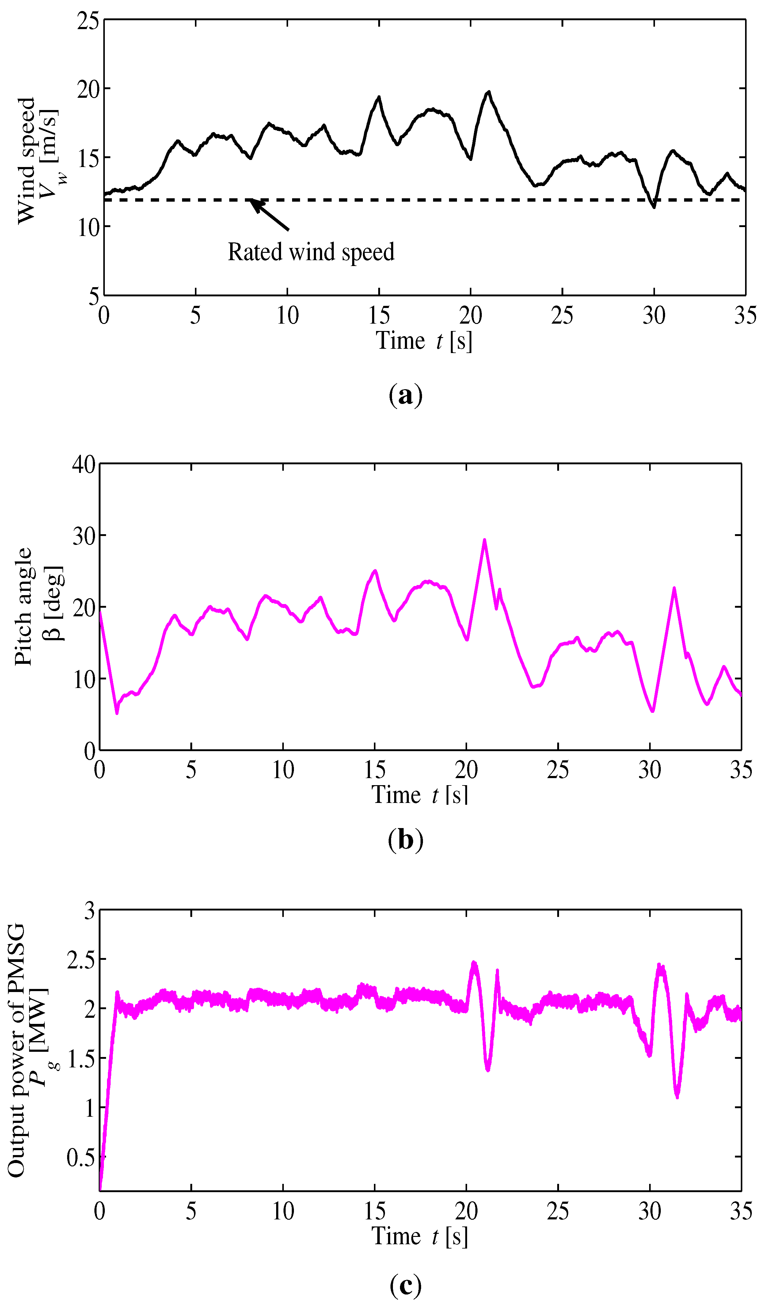
The external inputs (current references) and disturbances (decoupling components), w are may vary during the applications. To prove the robustness of the proposed $H_{\infty }$ controller, these inputs are measured under 10% error of estimation. The simulation results are shown in Figure 16. Figure 16a shows the wind speed. It is also a high turbulence wind speed. 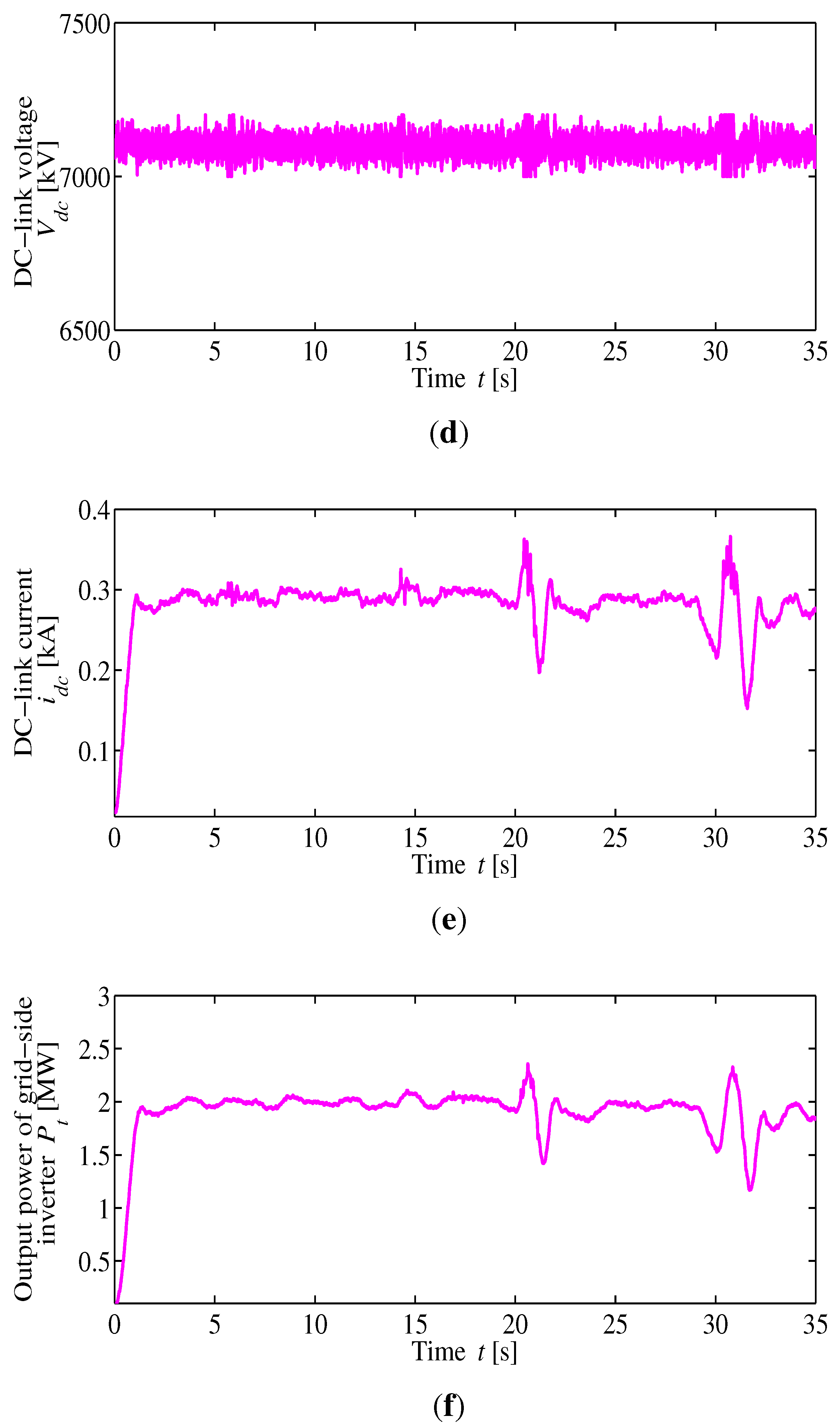The pitch angle of the WECS is shown in Figure 16b. The output power of the PMSG, DC-link voltage and DC-link current are shown in Figure 16c–e respectively. All simulation results show a good behavior. The output power of the grid-side inverter is shown in Figure 16f which also shows good behavior. On the other hand, simulation results show from the time 0s which includes the transient region of the wind turbine generation system. From the simulation results, the controller performances at transient regions are perfect.

Figure 16. Simulation Results (Robustness of the proposed system). (a) Wind speed; (b) Pitch angle; (c) Output power of PMSG; (d) DC-link voltage; (e) DC-link current; (f) Output power of grid-side inverter.

Figure 16. Simulation Results (Robustness of the proposed system). (a) Wind speed; (b) Pitch angle; (c) Output power of PMSG; (d) DC-link voltage; (e) DC-link current; (f) Output power of grid-side inverter.

From the above three different analyses, it is confirmed that when the wind speed becomes much higher than the rated speed, the conventional PI controller cannot control the large current and voltage accurately. The fuzzy controller requires additional adjustment for different levels of wind speeds. But the fuzzy controller method can improve performances as compared with the conventional PI controller method. The proposed digital $H_{\infty }$ robust controller can control the WECS perfectly any types of wind speeds.

6. Conclusions

Due to the uncertainties of the wind speed and increasing the rated power of the WECS, it is complicated to control the all operating regions through a conventional PI controller. In this paper, a new type of robust control methodology has been presented. Most of the wind energy researches have been proposed within a low turbulence wind velocities. So, it does not ensure the robust stabilities of the WECS. This paper shows the two different wind speeds and parameters error to establish the robust control abilities of the proposed method. From the simulation results, the proposed method can reduce the shaft stress, and the high frequency components of the DC-link voltage and current significantly as compared with the conventional PI controller method and the fuzzy controller method. Moreover, it can ensure the system stabilities during the high turbulence wind velocities. So, the proposed method can apply to any environment (low or high turbulence wind speeds) with a large capacity WECS. Also, the proposed digital $H_{\infty }$ controller can reduce the implementation complexities for a real system.

References

1. BP Statistical of World Energy June 2011. Available online: http://www.bp.com/statisticalreview (accessed on 20 March 2013).
2. Kaneko, T.; Uehara, A.; Senjyu, T.; Yona, A.; Urasaki, N. An integrated control method for a wind farm to reduce frequency deviations in a small power system. Appl. Energy 2011, 88, 1049–1058. [Google Scholar] [CrossRef]
3. Muhando, B.E.; Wies, R.W. Nonlinear H constrained feedback control for grid-interactive WECS under high stochasticity. IEEE Trans. Energy Convers. 2011, 26, 1000–1009. [Google Scholar] [CrossRef]
4. Uehara, A.; Pratap, A.; Goya, T.; Senjyu, T.; Yona, A.; Urasaki, N.; Funabashi, T. A coordinated control method to smooth wind power fluctuations of a PMSG-based WECS. IEEE Trans. Energy Convers. 2011, 26, 550–558. [Google Scholar] [CrossRef]
5. Kim, H.W.; Kim, S.S.; Ko, H.S. Modeling and control of PMSG-based variable-speed wind turbine. Electric Power Syst. Res. 2010, 80, 46–52. [Google Scholar] [CrossRef]
6. Howlader, A.M.; Urasaki, N.; Kousuke, U.; Yona, A.; Senjyu, T.; Kim, C.H.; Saber, A.Y. Parameter indentification of wind turbine for maximum power-point tracking control. Electr. Power Compon. Syst. 2010, 38, 603–614. [Google Scholar] [CrossRef]
7. Zhu, Y.; Cheng, M.; Hua, W.; Wang, W. DFIG-based wind power conversion with grid power leveling for reduced gusts. Energies 2012, 5, 1398–1412. [Google Scholar] [CrossRef]
8. Margaris, I.D.; Hansen, A.D.; Sorensen, P.; Hatziargyriou, N.D. Illustration of modern wind turbine ancillary services. Energies 2010, 2, 1290–1302. [Google Scholar] [CrossRef]
9. Howlader, A.M.; Urasaki, N.; Senjyu, T.; Uehara, A.; Yona, A.; Saber, A.Y. Output Power Smoothing of Wind Turbine Generation System for the 2-MW Permanent Magnet Synchronous Generators. In Proceedings of the 2010 International Conferences on Electrical Machine and Systems, Songdo, Korea, 10–13 October 2010; pp. 452–457.
10. Muhando, E.B.; Senjyu, T.; Uehara, A.; Funabashi, T.; Kim, C.H. LQG design for megawatt-class WECS with DFIG based on functional models fidelity prerequisites. IEEE Trans. Energy Convers. 2009, 24, 893–904. [Google Scholar] [CrossRef]
11. Rocha, R. A sensorless control for a variable speed wind turbine operating at partial load. Renew. Energy 2011, 36, 132–141. [Google Scholar] [CrossRef]
12. Howlader, A.M.; Urasaki, N.; Chakraborty, S.; Yona, A.; Senjyu, T.; Saber, A.Y. Fuzzy Controller Based Output Power Leveling Enhancement for a Permanent Magnet Synchronous Generator. In Proceedings of the 2011 IEEE International Conference on Fuzzy Systems, Taipe, Taiwan, 27–30 June 2011; pp. 656–661.
13. Galadi, V.; Piccolo, A.; Siano, A. Designing an adaptive fuzzy controller for maximum wind energy extraction. IEEE Trans. Energy Convers. 2008, 23, 559–569. [Google Scholar] [CrossRef]
14. Muhando, E.B.; Senjyu, T.; Uehara, A.; Funabashi, T. Gain-scheduled H control for WECS via LMI techniques and parametrically dependent feedback part I: Model development fundamentals. IEEE Trans. Ind. Electron. 2011, 58, 48–56. [Google Scholar] [CrossRef]
15. Muhando, E.B.; Senjyu, T.; Uehara, A.; Funabashi, T. Gain-scheduled H control for WECS via LMI techniques and parametrically dependent feedback part II: Controller design and implementation. IEEE Trans. Ind. Electron. 2011, 58, 57–65. [Google Scholar] [CrossRef]
16. Yao, X.J.; Guo, C.C.; Li, Y. LPV H-Infinity Controller Design for Variable-Pitch Variable-Speed Wind Turbine. In Proceedings of the IEEE 6th International Power Electronics and Motion Control Conference, Wuhan, China, 17–20 May 2009; pp. 2222–2227.
17. Deng, Y.; Zhou, J. LPV H-Infinity Controller Design for a Wind Power Generator. In Proceedings of the IEEE Conference on Robotics, Automation and Mechatronics, Chengdu, China, 21–24 September 2008; pp. 873–878.
18. Gu, D.W.; Petkov, P.R.; Konstantinov, M.M. Robust Control Design with MATLAB; Springer: Heidelberg, Germany, 2005. [Google Scholar]
19. Howlader, A.M.; Urasaki, N.; Yona, A.; Senjyu, T.; Kim, C.H.; Saber, A.Y. Output power leveling of a wind generation system using inertia of a wind turbine. Int. J. Emerg. Electr. Power Syst. 2009, 10, 1–13. [Google Scholar] [CrossRef]
20. Howlader, A.M.; Urasaki, N.; Yona, A.; Senjyu, T.; Funabashi, T.; Saber, A.Y. Output Power Leveling of Wind Generation System Using Inertia for PM Synchronous Generator. In Proceedings of the IEEE 8th International Conference on Power Electronics and Drive Systems, Taipe, Taiwan, 2–5 November 2009; pp. 1289–1294.