The Effect of Free-Atmosphere Stratification on Boundary-Layer Flow and Power Output from Very Large Wind Farms


Abstract
:
1. Introduction
2. Large-Eddy Simulation Framework
2.1. LES Governing Equations
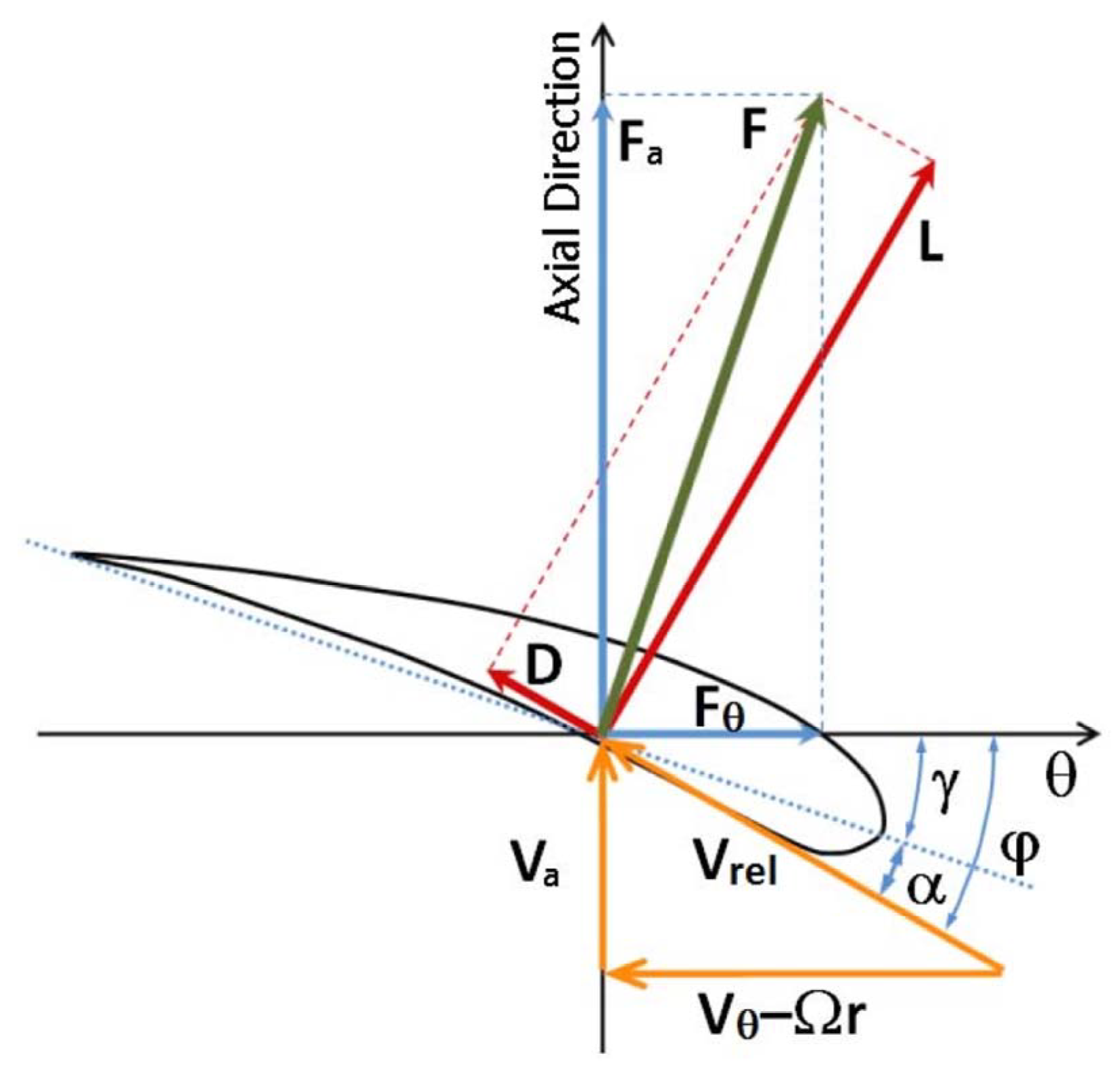
2.2. Wind-Turbine Parameterization

2.3. Numerical Setup

| Case | zo (m) | Abbreviation | Γ (K/km) | Number of wind turbines (Ntx × Nty) | sx × sy | Turbine arrangement | Lx × Ly × Lz (m3) | Nx × Ny × Nz |
|---|---|---|---|---|---|---|---|---|
| A1 | 0.1 | − | 1 | No farm | − | − | 3906 × 3255 × 1045 | 126 × 175 × 80 |
| A2 | 0.01 | − | 1 | No farm | − | − | 3906 × 3255 × 1045 | 126 × 175 × 80 |
| A3 | 0.1 | − | 10 | No farm | − | − | 3906 × 3255 × 1045 | 126 × 175 × 80 |
| A4 | 0.01 | − | 10 | No farm | − | − | 3906 × 3255 × 1045 | 126 × 175 × 80 |
| B1 | 0.1 | s5 × 5 − Γ1 | 1 | 8 × 7 | 5 × 5 | Staggered | 3720 × 3255 × 1687 | 126 × 175 × 128 |
| B2 | 0.1 | a5 × 5 − Γ1 | 1 | 8 × 7 | 5 × 5 | Aligned | 3720 × 3255 × 1687 | 126 × 175 × 128 |
| C1 | 0.1 | s5 × 5 − Γ10 | 10 | 8 × 7 | 5 × 5 | Staggered | 3720 × 3255 × 1045 | 126 × 175 × 80 |
| C2 | 0.1 | a5 × 5 − Γ10 | 10 | 8 × 7 | 5 × 5 | Aligned | 3720 × 3255 × 1045 | 126 × 175 × 80 |
| D1 | 0.1 | s7 × 7 − Γ1 | 1 | 6 × 5 | 7 × 7 | Staggered | 3906 × 3255 × 1687 | 126 × 175 × 128 |
| D2 | 0.1 | a7 × 7 − Γ1 | 1 | 6 × 5 | 7 × 7 | Aligned | 3906 × 3255 × 1687 | 126 × 175 × 128 |
| E1 | 0.1 | s7 × 7 − Γ10 | 10 | 6 × 5 | 7 × 7 | Staggered | 3906 × 3255 × 1045 | 126 × 175 × 80 |
| E2 | 0.1 | a7 × 7 − Γ10 | 10 | 6 × 5 | 7 × 7 | Aligned | 3906 × 3255 × 1045 | 126 × 175 × 80 |
3. LES Results
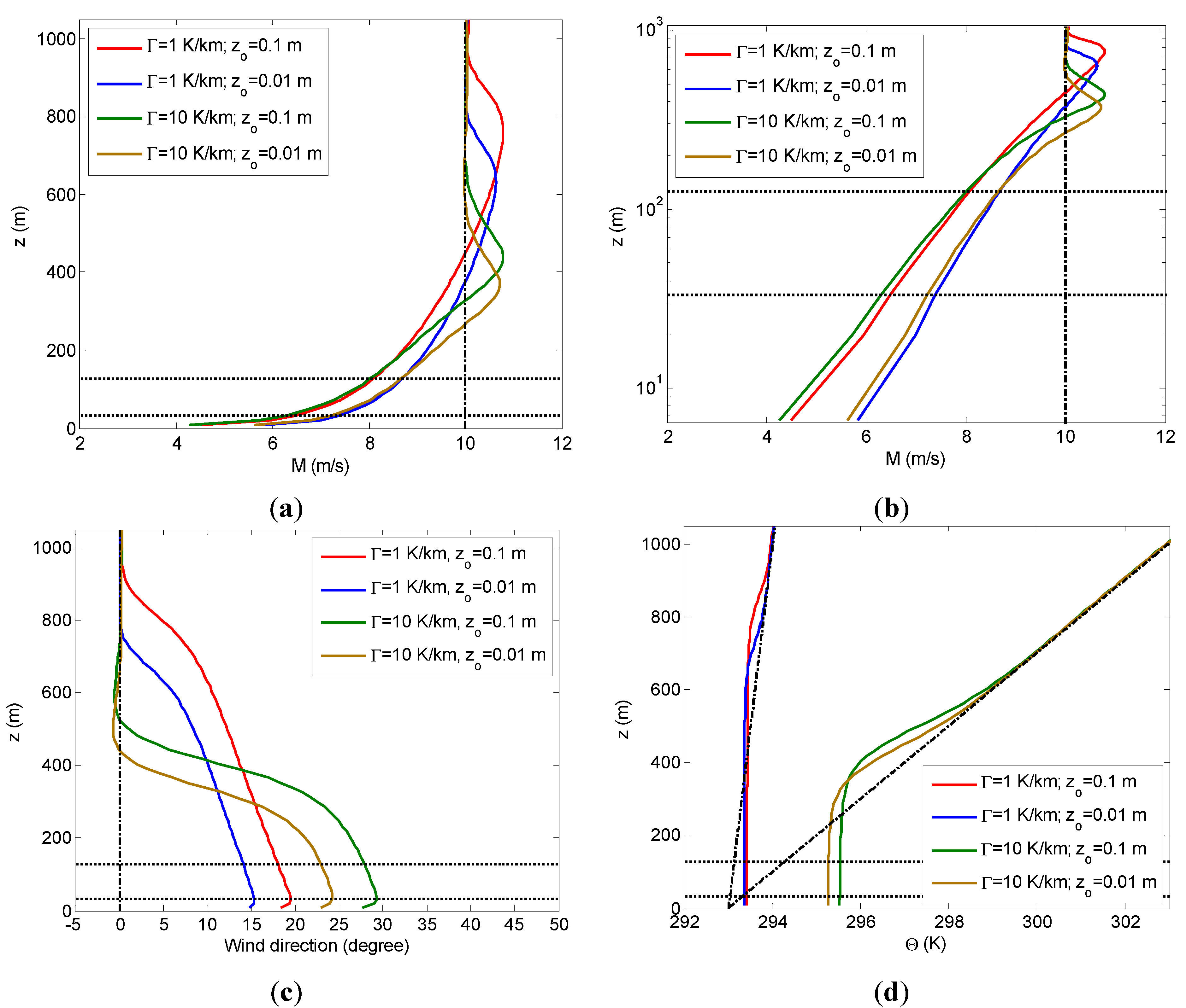
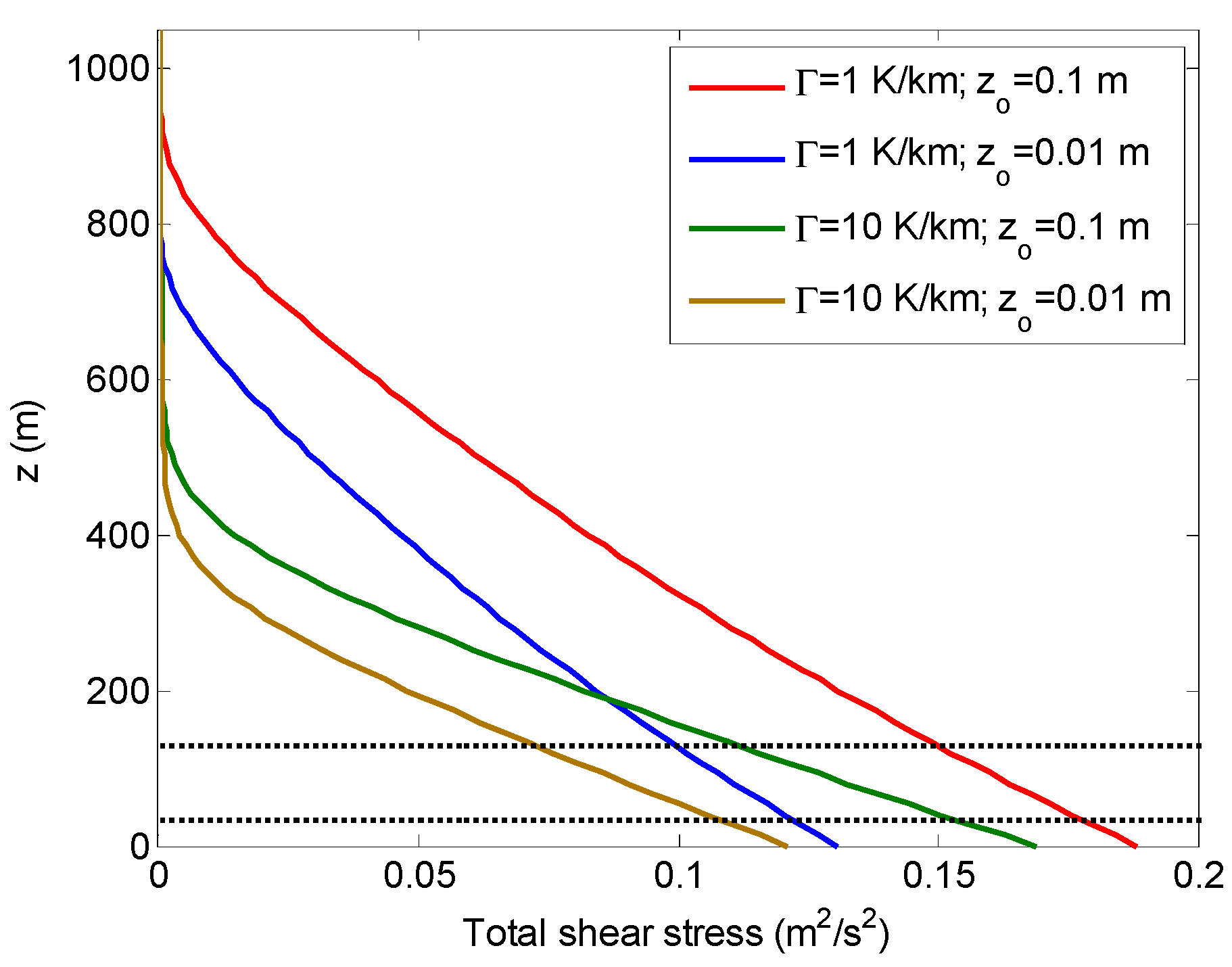
3.1. No-Farm Case


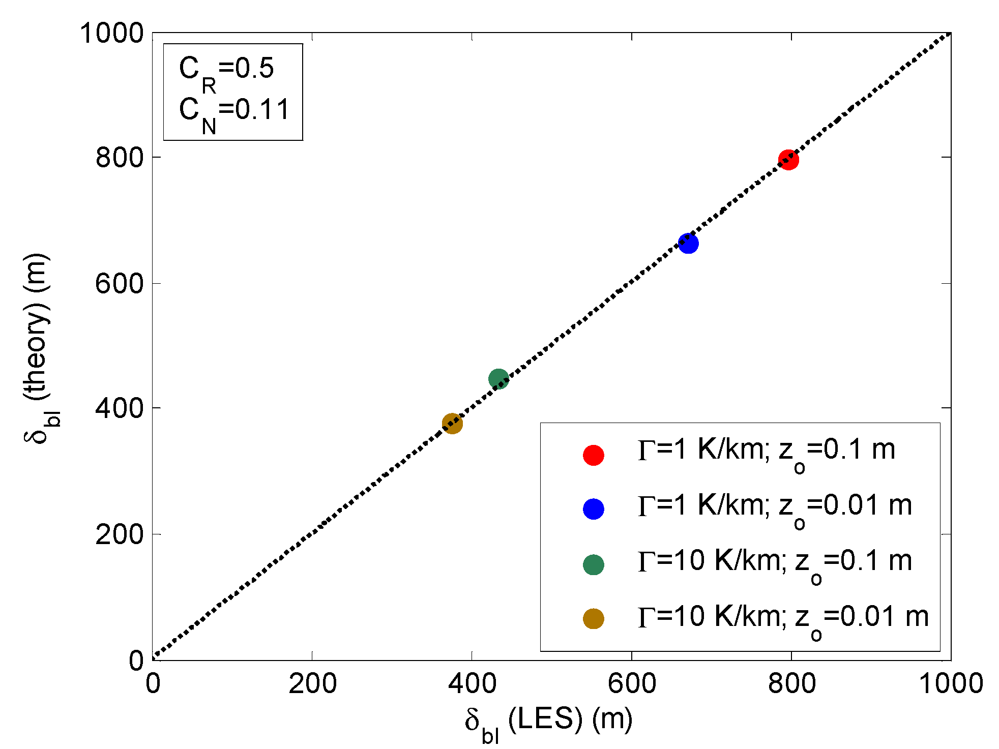
3.1.1. The Effect of Free-Atmosphere Stability on the ABL Depth


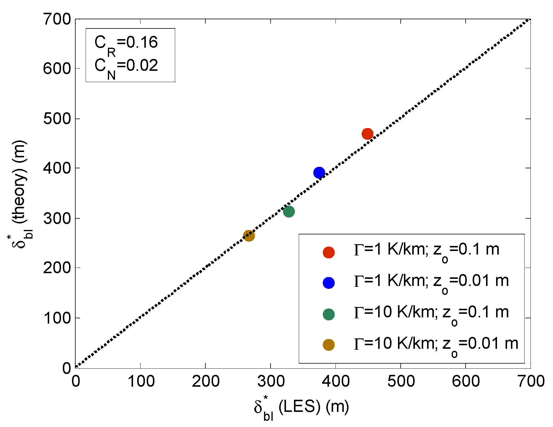
3.1.2. The Effect of Free-Atmosphere Stability on the Surface-Layer Parameterization
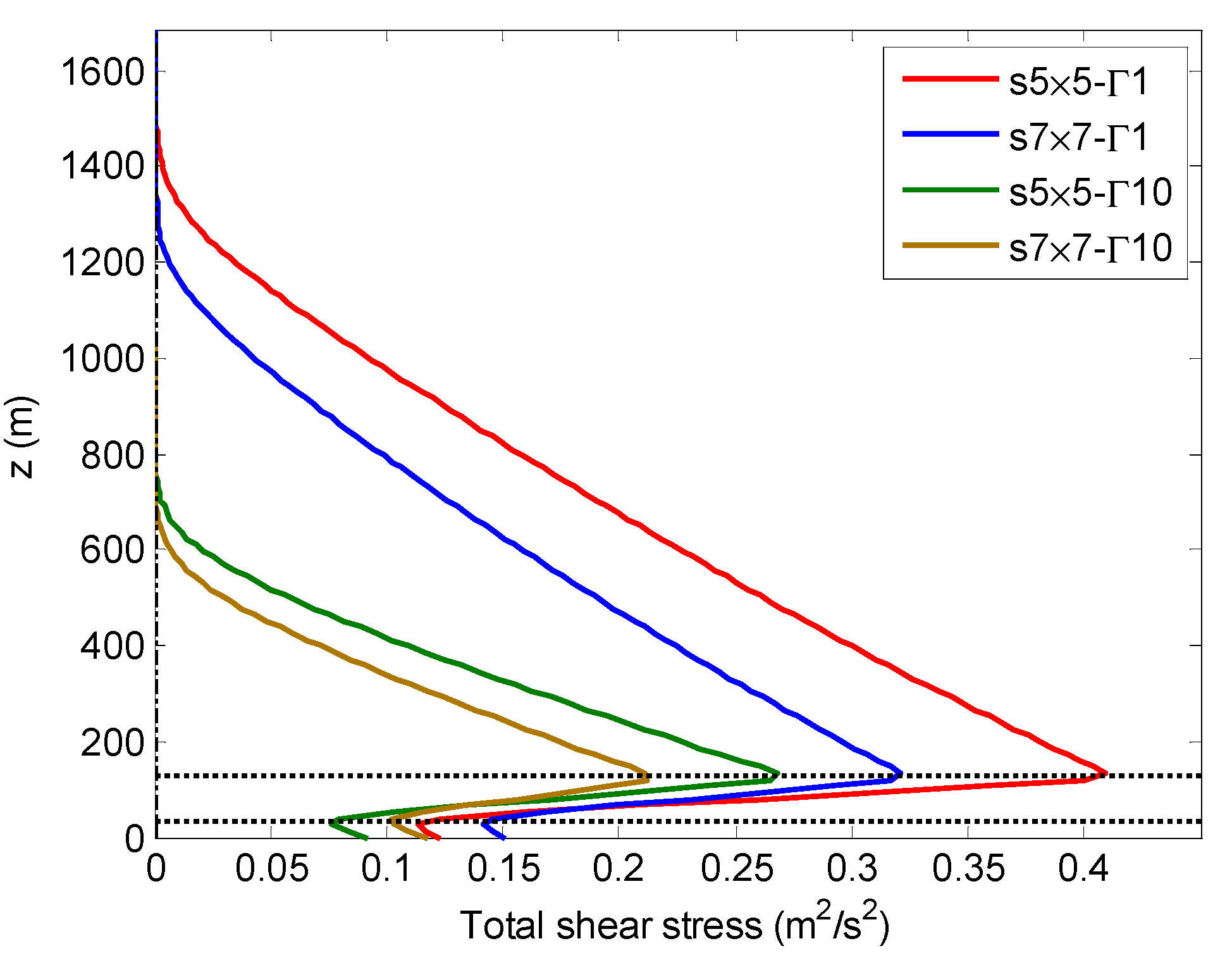
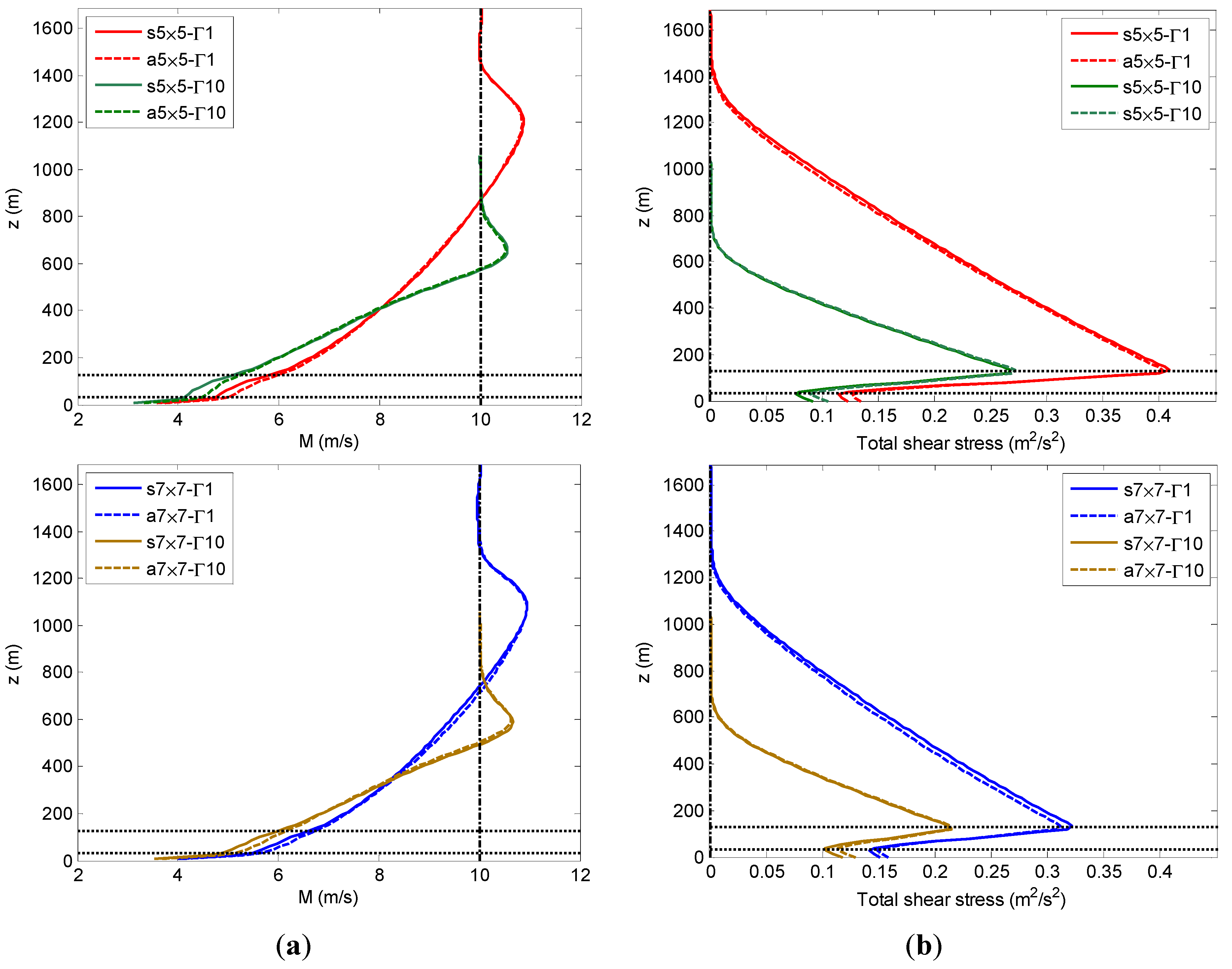
3.2. Wind-Farm Case


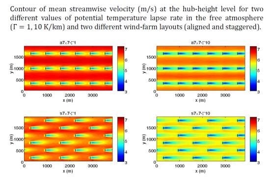
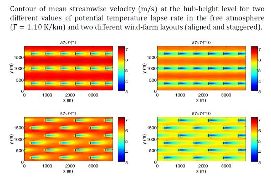
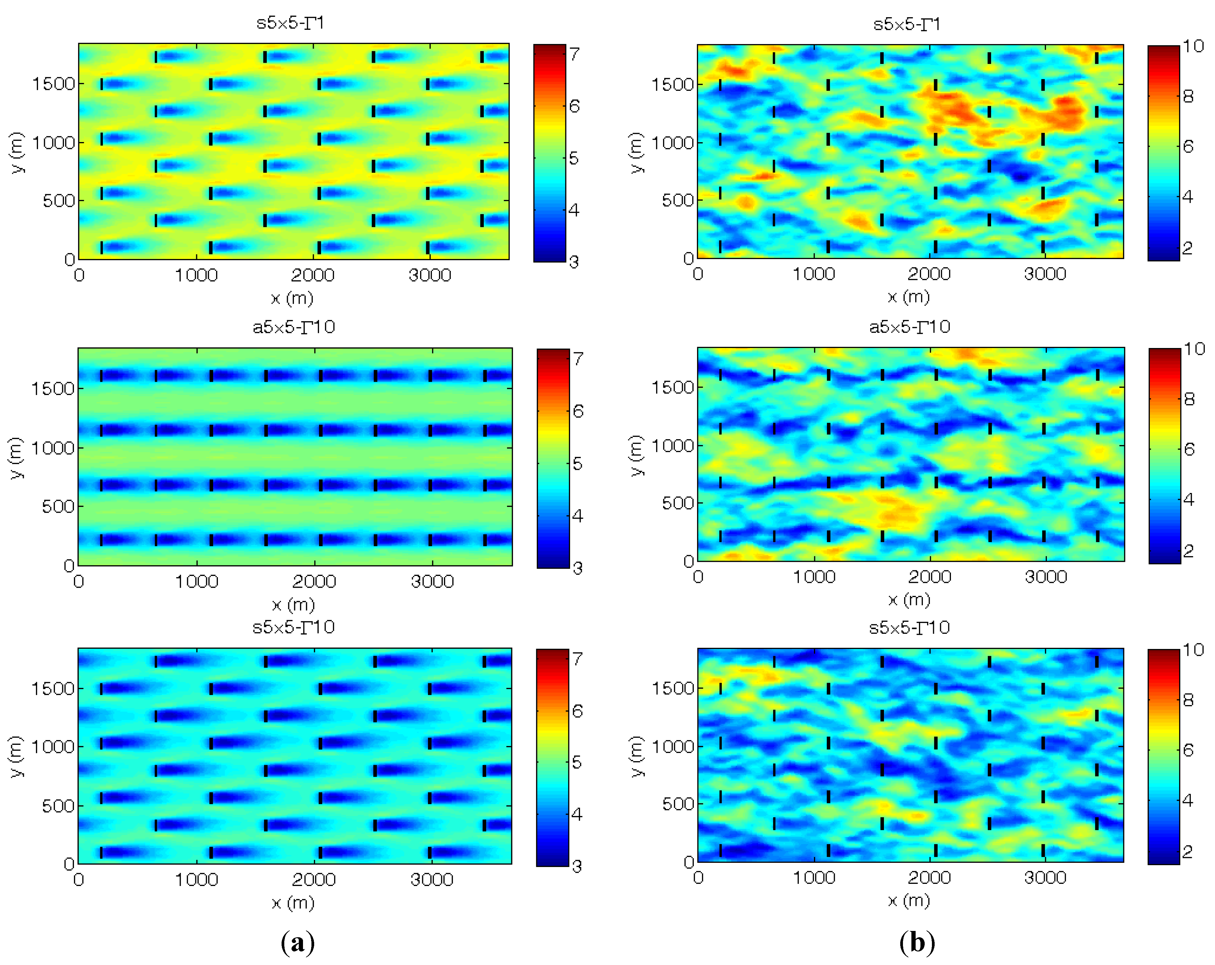
3.3. Layout Effect

| Case | Power/Turbine (MW) |
|---|---|
| s5 × 5 − Γ1 | 0.3069 |
| a5 × 5 − Γ1 | 0.2835 |
| s5 × 5 − Γ10 | 0.1995 |
| a5 × 5 − Γ10 | 0.1841 |
| s7 × 7 − Γ1 | 0.4303 |
| a7 × 7 − Γ1 | 0.3811 |
| s7 × 7 − Γ10 | 0.2993 |
| a7 × 7 − Γ10 | 0.2690 |


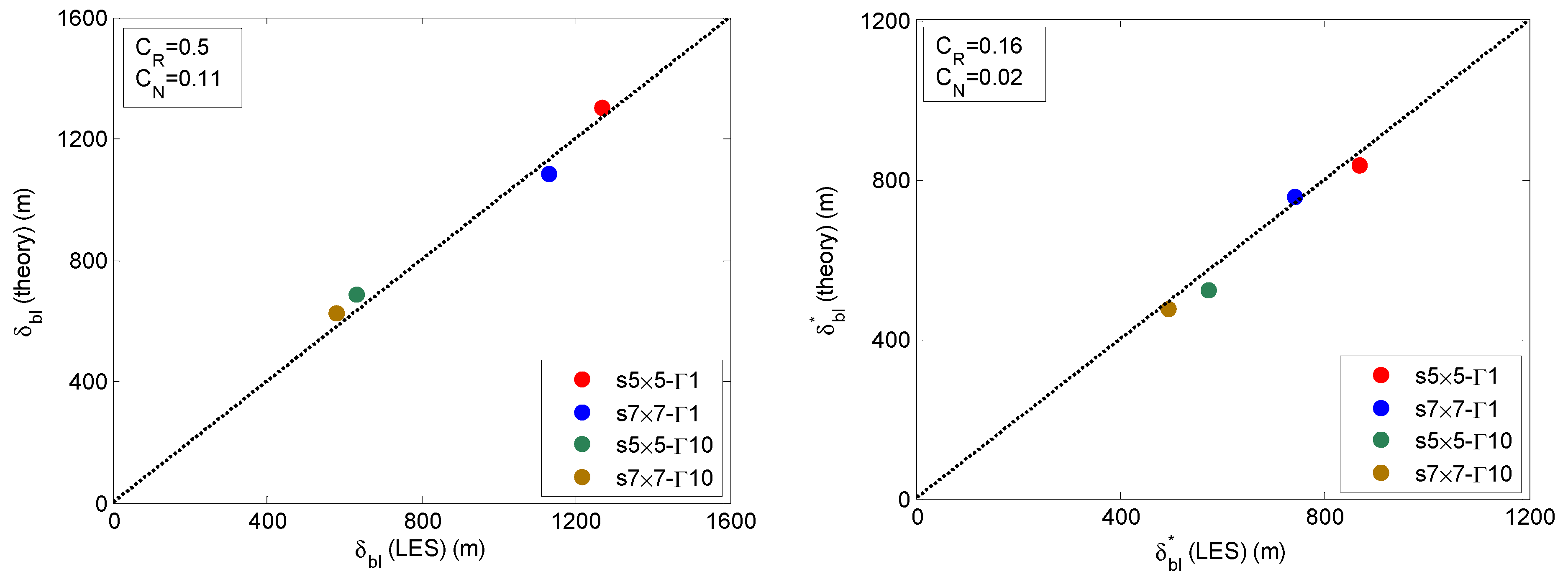
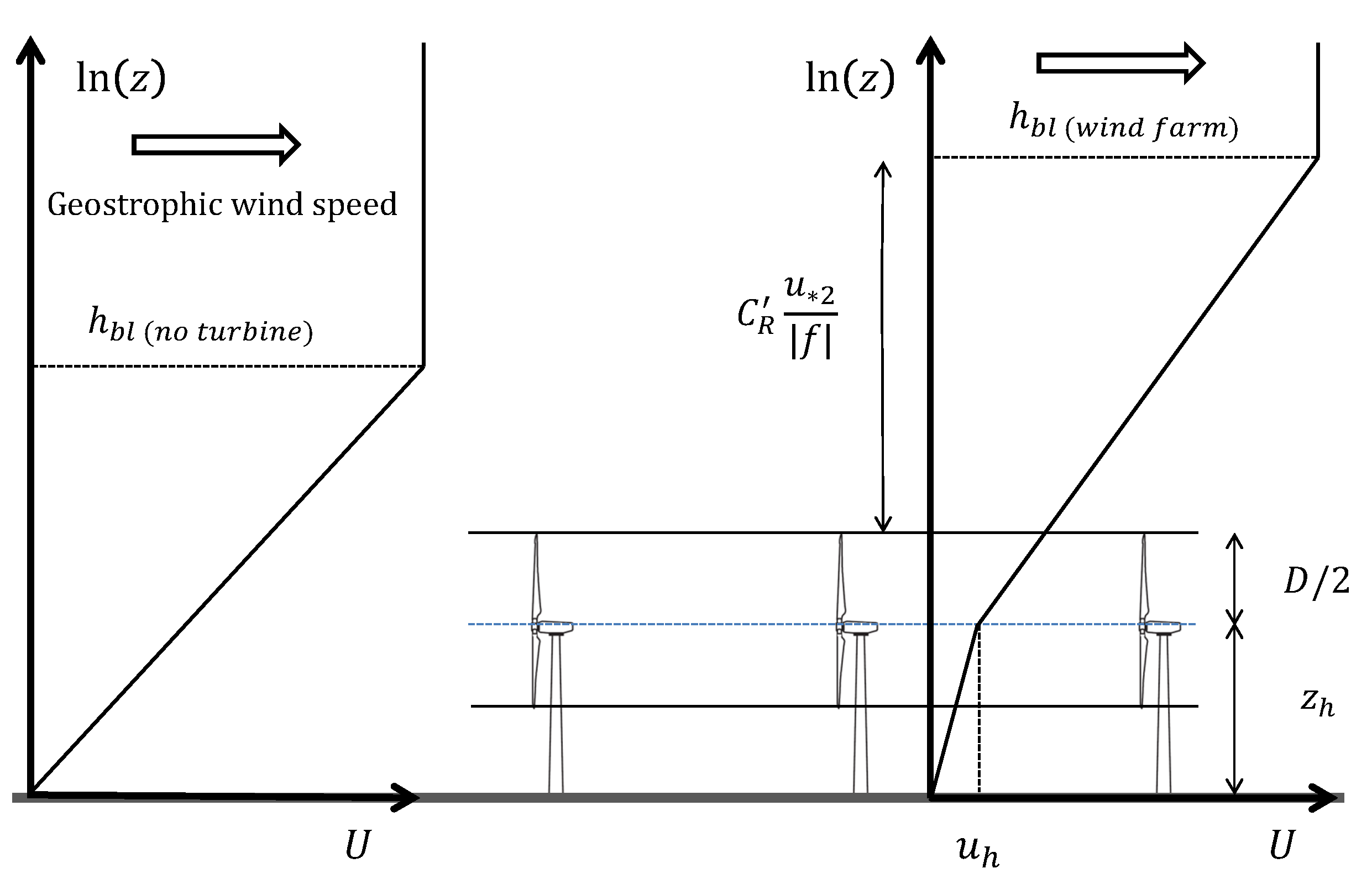
4. One-Dimensional (1D) Modeling of Very Large Wind Farms in Conventionally Neutral Conditions

| Case | a | ||
|---|---|---|---|


5. Conclusions
Acknowledgments
References
- Frandsen, S. On the wind speed reduction in the center of large clusters of wind turbines. J. Wind Eng. Ind. Aerodyn. 1992, 39, 251–265. [Google Scholar] [CrossRef]
- Calaf, M.; Meneveau, C.; Meyers, J. Large eddy simulation study of fully developed wind turbine array boundary layers. Phys. Fluids 2010, 22, 015110:1–01511016. [Google Scholar] [CrossRef]
- Meneveau, C. The top-down model of wind farm boundary layers and its applications. J. Turbul. 2012, 13, 1–12. [Google Scholar] [CrossRef]
- Lu, H.; Porté-Agel, F. Large-eddy simulation of a very large wind farm in a stable atmospheric boundary layer. Phys. Fluids 2011, 23, 065101:1–065101:19. [Google Scholar]
- Johnstone, R.; Coleman, G.N. The turbulent Ekman boundary layer over an infinite wind-turbine array. J. Wind Eng. Ind. Aerodyn. 2012, 100, 46–57. [Google Scholar] [CrossRef]
- Zilitinkevich, S.; Esau, I.; Baklanov, A. Further comments on the equilibrium height of neutral and stable planetary boundary layers. Q. J. R. Meteorol. Soc. 2007, 133, 265–271. [Google Scholar] [CrossRef]
- Zilitinkevich, S.; Baklanov, A.; Rost, J.; Smedman, A.; Lykosov, V.; Calanca, P. Diagnostic and prognostic equations for the depth of the stably stratified Ekman boundary layer. Q. J. R. Meteorol. Soc. 2002, 128, 25–46. [Google Scholar] [CrossRef]
- Zilitinkevich, S.; Esau, I. On integral measures of the neutral, barotropic planetary boundary layers. Bound. Layer Meteorol. 2002, 104, 371–379. [Google Scholar] [CrossRef]
- Esau, I. Parameterization of a surface drag coefficient in conventionally neutral planetary boundary layer. Ann. Geophys. 2004, 22, 3353–3362. [Google Scholar] [CrossRef]
- Taylor, J.; Sarkar, S.; Armenio, V. Large eddy simulation of stably stratified open channel flow. Phys. Fluids 2005, 17, 116602. [Google Scholar] [CrossRef]
- Taylor, J.; Sarkar, S. Direct and large eddy simulations of a bottom Ekman layer under an external stratification. Int. J. Heat Fluid Flow 2008, 29, 721–732. [Google Scholar] [CrossRef]
- Sorbjan, Z. Effects caused by varying the strength of the capping inversion based on a large eddy simulation model of the shear-free convective boundary layer. J. Atmos. Sci. 1996, 53, 2015–2024. [Google Scholar] [CrossRef]
- Stoll, R.; Porté-Agel, F. Dynamic subgrid-scale models for momentum and scalar fluxes in large-eddy simulations of neutrally stratified atmospheric boundary layers over heterogeneous terrain. Water Resour. Res. 2006, 42, W01409. [Google Scholar] [CrossRef]
- Wu, Y.-T.; Porté-Agel, F. LES of wind-turbine wakes: Evaluation of turbine parameterizations. Bound. Layer Meteorol. 2011, 138, 345–366. [Google Scholar] [CrossRef]
- Smagorinsky, J. General circulation experiments with the primitive equations: I. The basic experiment. Mon. Weather Rev. 1963, 91, 99–164. [Google Scholar] [CrossRef]
- Germano, M.; Piomelli, U.; Moin, P. A dynamic subgrid-scale eddy viscosity model. Phys. Fluids 1991, 7, 1760–1765. [Google Scholar] [CrossRef]
- Moin, P.; Squires, K.D.; Lee, S. A dynamic subgrid-scale model for compressible turbulence and scalar transport. Phys. Fluids 1991, 3, 2746–2757. [Google Scholar] [CrossRef]
- Porté-Agel, F.; Meneveau, C.; Parlange, M.B. A scale-dependent dynamic model for large-eddy simulation: Application to a neutral atmospheric boundary layer. J. Fluid Mech. 2000, 415, 261–284. [Google Scholar] [CrossRef]
- Porté-Agel, F. A scale-dependent dynamic model for scalar transport in large-eddy simulations of the atmospheric boundary layer. Bound. Layer Meteorol. 2004, 112, 81–105. [Google Scholar] [CrossRef]
- Stoll, R.; Porté-Agel, F. Surface heterogeneity effects on regional-scale fluxes in stable boundary layers: Surface temperature transitions. J. Atmos. Sci. 2008, 66, 412–431. [Google Scholar] [CrossRef]
- Stoll, R.; Porté-Agel, F. Large-eddy simulation of the stable atmospheric boundary layer using dynamic models with different averaging schemes. Bound. Layer Meteorol. 2008, 126, 1–28. [Google Scholar] [CrossRef]
- Wan, F.; Porté-Agel, F.; Stoll, R. Evaluation of dynamic subgrid-scale models in large-eddy simulations of neutral turbulent flow over a two dimensional sinusoidal hill. Atmos. Environ. 2007, 41, 2719–2728. [Google Scholar] [CrossRef]
- Wan, F.; Porté-Agel, F. Large-eddy simulation of stably-stratified flow over a steep hill. Bound. Layer Meteorol. 2011, 138, 367–384. [Google Scholar] [CrossRef]
- Wu, Y.-T.; Porté-Agel, F. Simulation of turbulent flow inside and above wind farms: Model validation and layout effects. Bound. Layer Meteorol. 2013, 146, 181–205. [Google Scholar] [CrossRef]
- Porté-Agel, F.; Wu, Y.-T.; Lu, H.; Conzemius, R.J. Large-eddy simulation of atmospheric boundary layer flow through wind turbines and wind farms. J. Wind Eng. Ind. Aerodyn. 2011, 99, 154–168. [Google Scholar] [CrossRef]
- Albertson, J.D.; Parlange, M.B. Natural integration of scalar fluxes from complex terrain. Adv. Water Resour. 1999, 23, 239–252. [Google Scholar] [CrossRef]
- Orszag, S.A. Transform method for calculation of vector coupled sums: Application to the spectral form of the vorticity equation. J. Atmos. Sci. 1970, 27, 890–895. [Google Scholar] [CrossRef]
- Canuto, C.; Hussaini, M.Y.; Quarteroni, A.; Zang, T.A. Spectral Methods in Fluid Dynamics; Springer: Berlin, Germany, 1988. [Google Scholar]
- Monin, A.; Obukhov, M. Basic laws of turbulent mixing in the ground layer of the atmosphere. Trans. Geophys. Inst. Akad. Nauk. 1954, 151, 163–187. [Google Scholar]
- Marusic, I.; Kunkel, G.J.; Porté-Agel, F. Experimental study of wall boundary conditions for large-eddy simulation. J. Fluid. Mech. 2001, 446, 309–320. [Google Scholar]
- Abkar, M.; Porté-Agel, F. A new boundary condition for large-eddy simulation of boundary-layer flow over surface roughness transitions. J. Turbul. 2012, 13, 1–18. [Google Scholar] [CrossRef]
- Rossby, C.G.; Montgomery, R.B. The layers of frictional influence in wind and ocean currents. Phys. Oceanogr. Meteorol. 1935, 3, 1–101. [Google Scholar]
- Zilitinkevich, S.; Esau, I. The effect of baroclinicity on the depth of neutral and stable planetary boundary layers. Q. J. R. Meteorol. Soc. 2003, 129, 3339–3356. [Google Scholar] [CrossRef]
- Blackadar, A.K. The vertical distribution of wind and turbulent exchange in a neutral atmosphere. J. Geophys. Res. 1962, 67, 3095–3102. [Google Scholar] [CrossRef]
- Holt, T.; Raman, S. A review and comparative evaluation of multilevel boundary layer parameterizations for first-order and turbulent kinetic energy closure schemes. Rev. Geophys. 1988, 26, 761–780. [Google Scholar] [CrossRef]
- Mason, P.J.; Thompson, D.J. Stochastic backscatter in large-eddy simulations of boundary layers. J. Fluid Mech. 1992, 242, 51–78. [Google Scholar] [CrossRef]
- Zilitinkevich, S.; Perov, V.; King, J. Near-surface turbulent fluxes in stable stratification: Calculation for use in general circulation models. Q. J. R. Meteorol. Soc. 2002, 128, 1571–1587. [Google Scholar] [CrossRef]
- Meyers, J.; Meneveau, C. Large Eddy Simulations of Large Wind-Turbine Arrays in the Atmospheric Boundary Layer. In Proceedings of the 48th AIAA Aerospace Sciences Meeting Including the New Horizons Forum and Aerospace Exposition, Orlando, FL, USA, 4–7 January 2010. AIAA2010-827.
- Markfort, C.D.; Zhang, W.; Porté-Agel, F. Turbulent flow and scalar transport through and over aligned and staggered wind farms. J. Turbul. 2012, 13, 1–36. [Google Scholar] [CrossRef]
- Yang, X.; Kang, S.; Sotiropoulos, F. Computational study and modeling of turbine spacing effects in infinite aligned wind farms. Phys. Fluids. 2012, 24, 115107:1–115107:28. [Google Scholar]
- Meyers, J.; Meneveau, C. Optimal turbine spacing in fully developed wind farm boundary layers. Wind Energy 2011, 15, 305–317. [Google Scholar] [CrossRef]
- Tennekes, H.; Lumley, J.L. A First Course in Turbulence; MIT Press: Cambridge, MA, USA, 1972. [Google Scholar]
© 2013 by the authors; licensee MDPI, Basel, Switzerland. This article is an open access article distributed under the terms and conditions of the Creative Commons Attribution license (http://creativecommons.org/licenses/by/3.0/).
Share and Cite
Abkar, M.; Porté-Agel, F. The Effect of Free-Atmosphere Stratification on Boundary-Layer Flow and Power Output from Very Large Wind Farms. Energies 2013, 6, 2338-2361. https://0-doi-org.brum.beds.ac.uk/10.3390/en6052338
Abkar M, Porté-Agel F. The Effect of Free-Atmosphere Stratification on Boundary-Layer Flow and Power Output from Very Large Wind Farms. Energies. 2013; 6(5):2338-2361. https://0-doi-org.brum.beds.ac.uk/10.3390/en6052338
Chicago/Turabian StyleAbkar, Mahdi, and Fernando Porté-Agel. 2013. "The Effect of Free-Atmosphere Stratification on Boundary-Layer Flow and Power Output from Very Large Wind Farms" Energies 6, no. 5: 2338-2361. https://0-doi-org.brum.beds.ac.uk/10.3390/en6052338