Online Semiparametric Identification of Lithium-Ion Batteries Using the Wavelet-Based Partially Linear Battery Model

Abstract
:1. Introduction
2. Modeling of the Lithium-Ion Battery
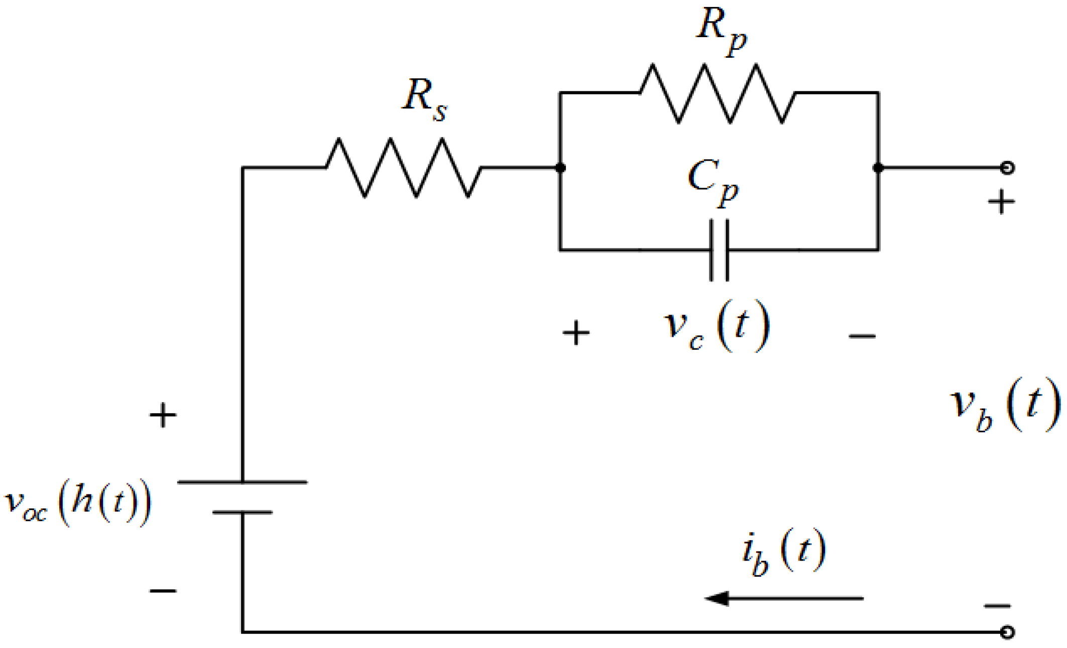
2.1. Battery Equivalent Circuit Equations

2.2. PLBM
3. Online Identification of the Wavelet-Based PLBM
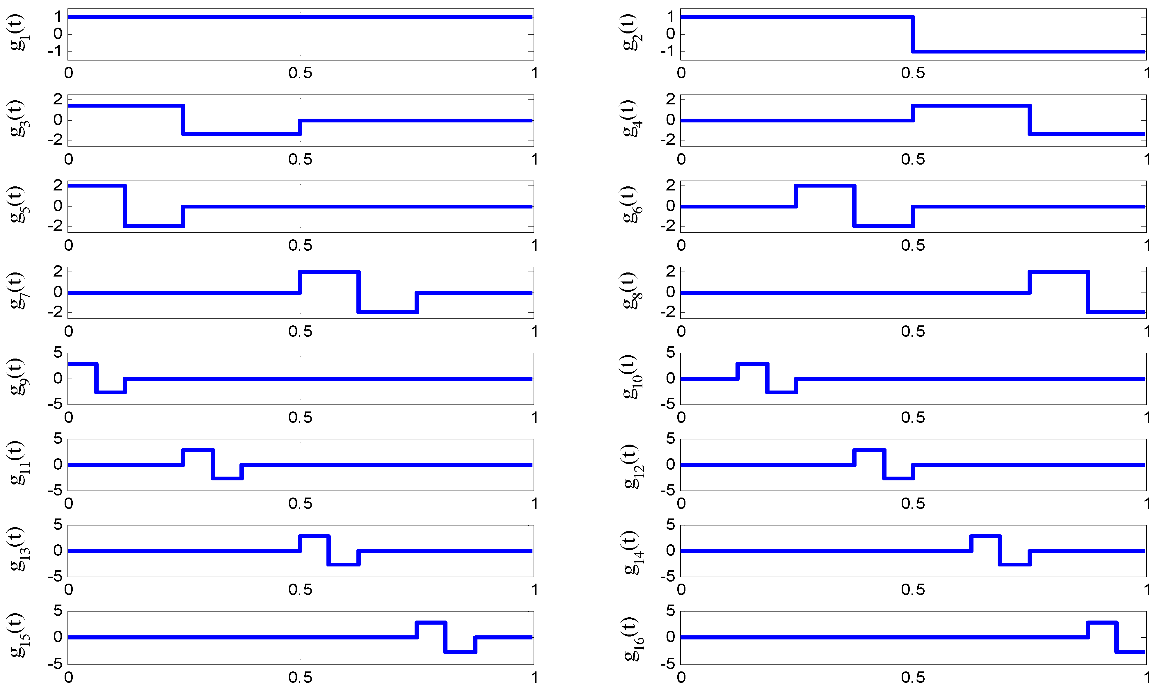
3.1. Wavelet MRA
3.2. Truncated Wavelet MRA Expansion of the Nonparametric Component

3.3. Recursive Penalized Wavelet Estimator for Online PLBM Identification

4. Simulation and Experimental Results
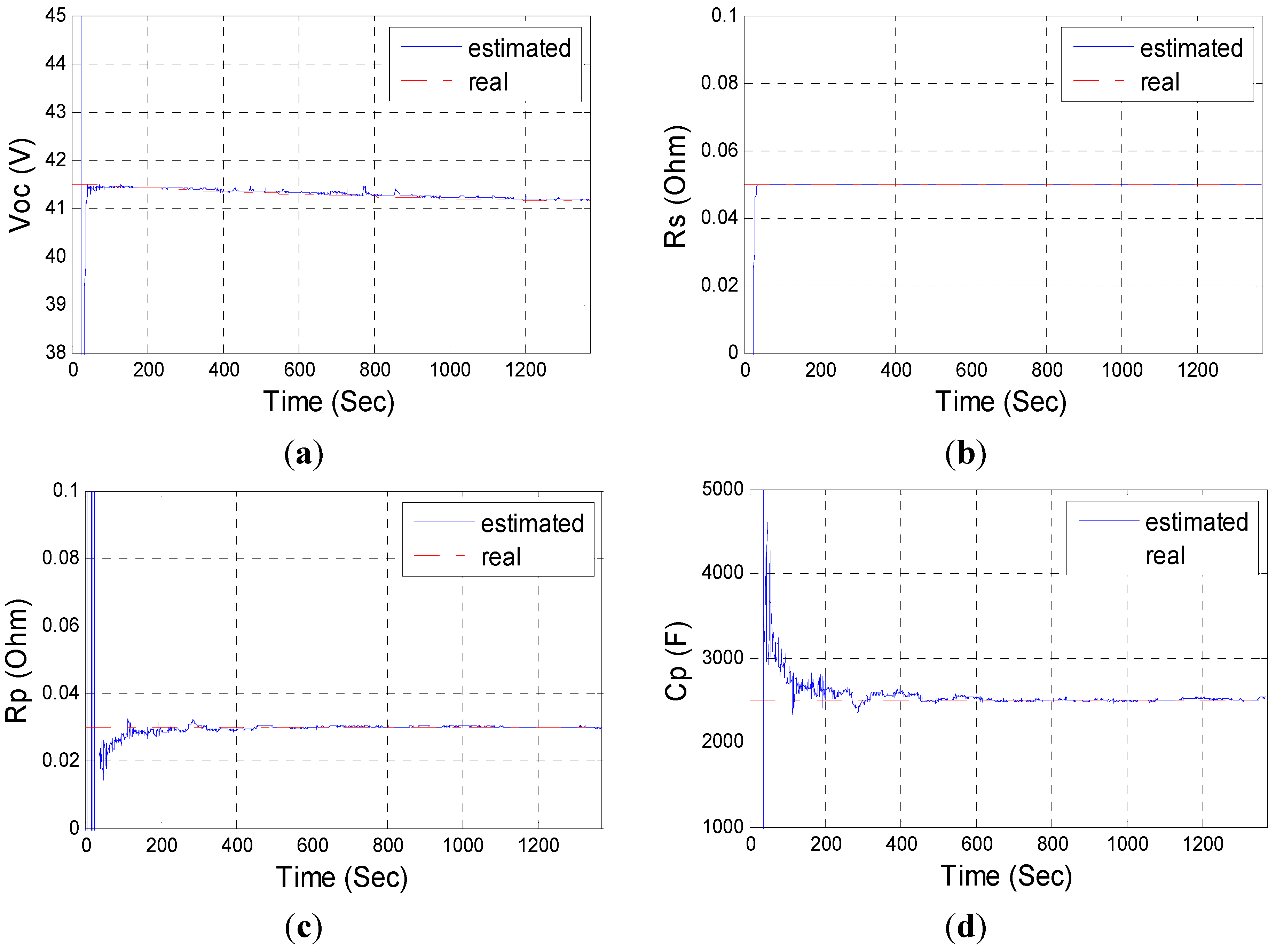
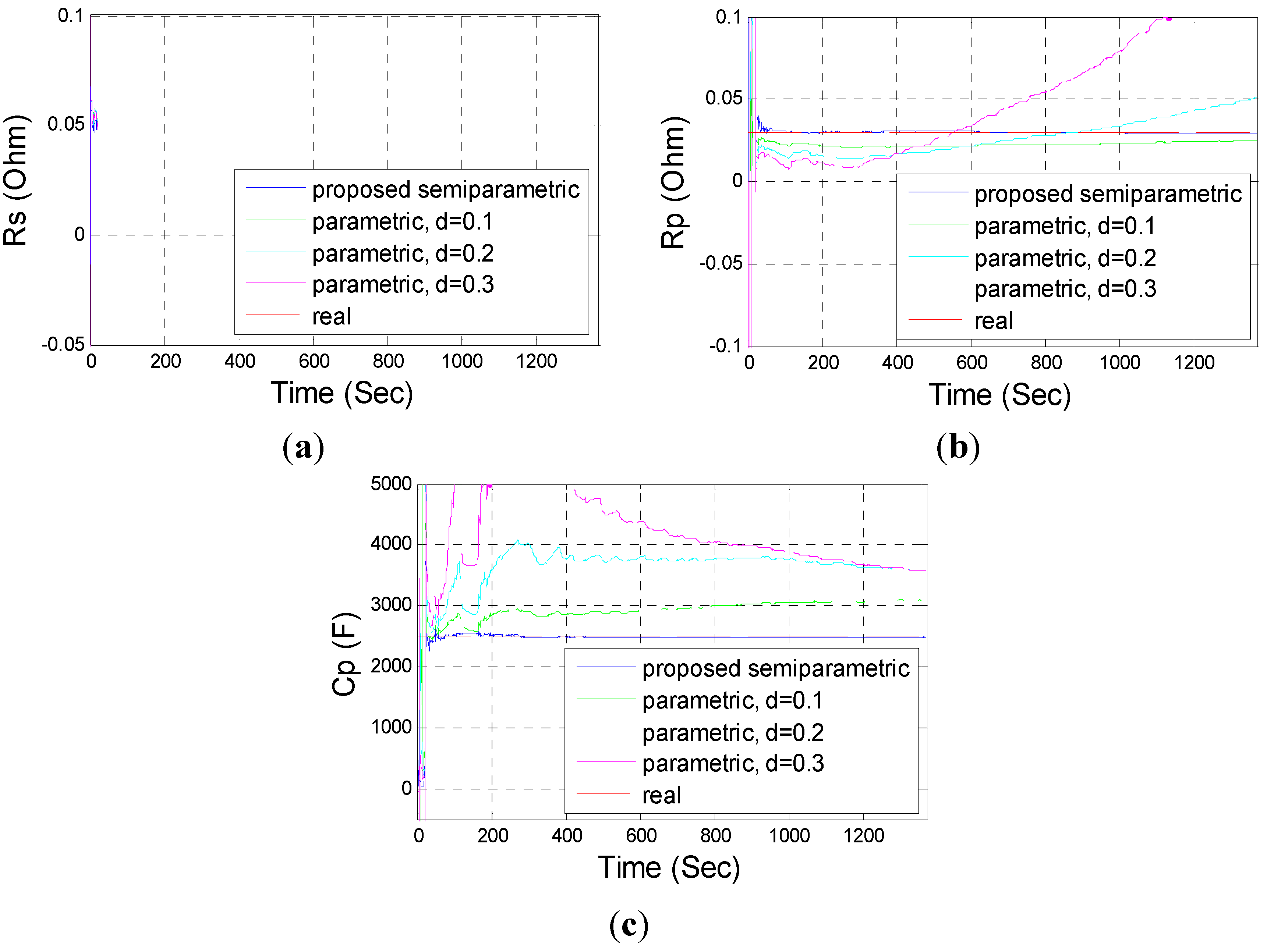
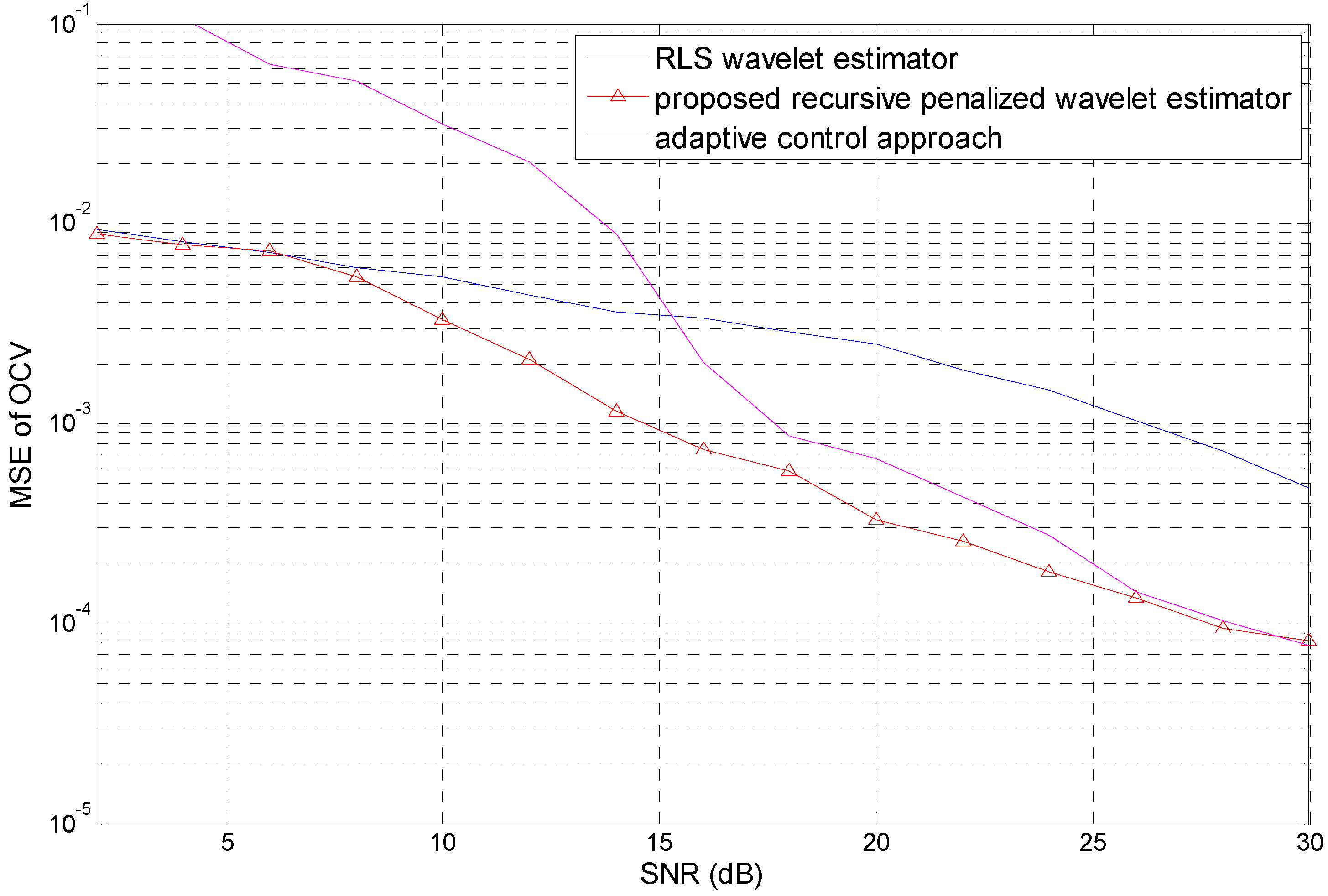
4.1. Simulations


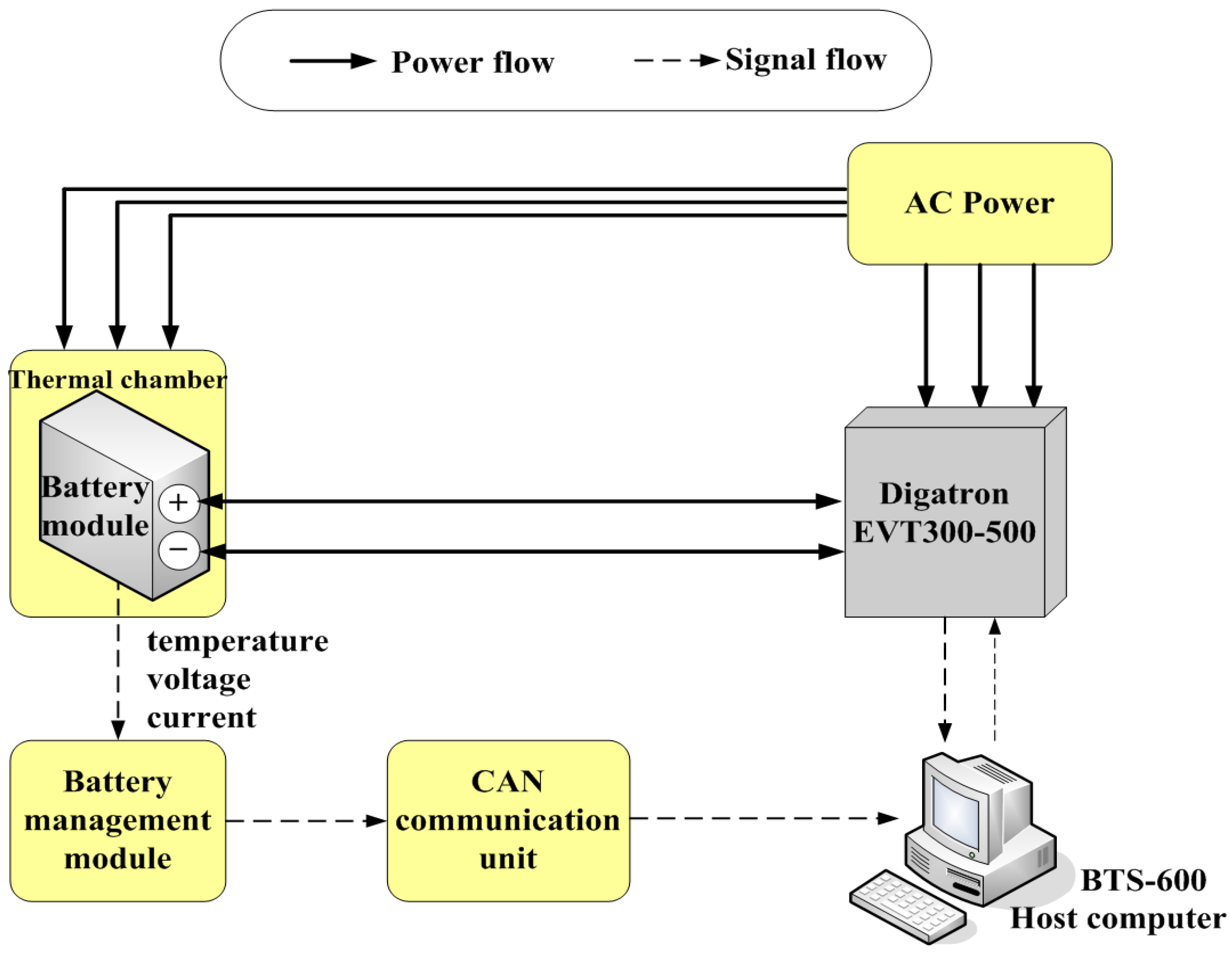
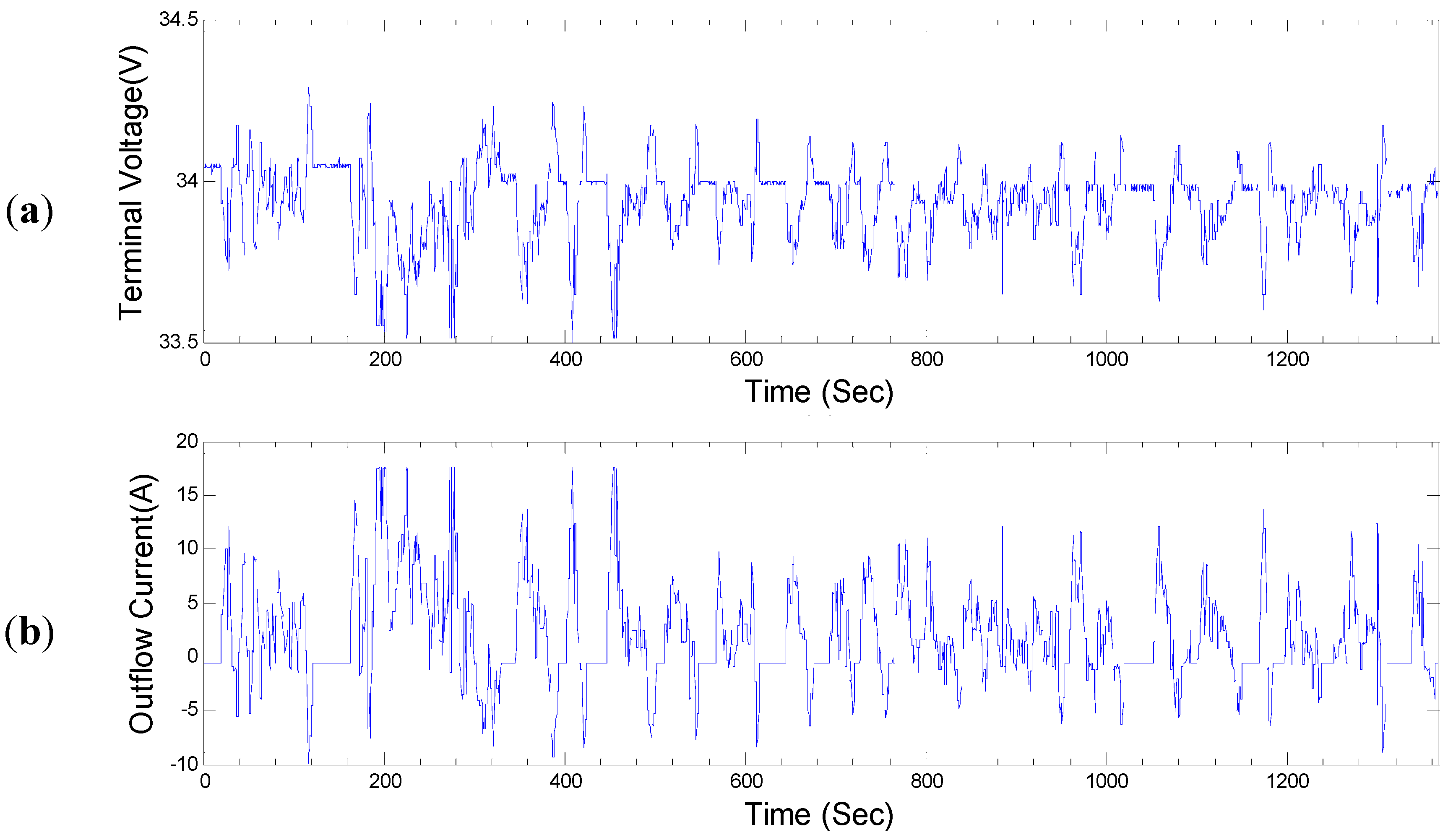
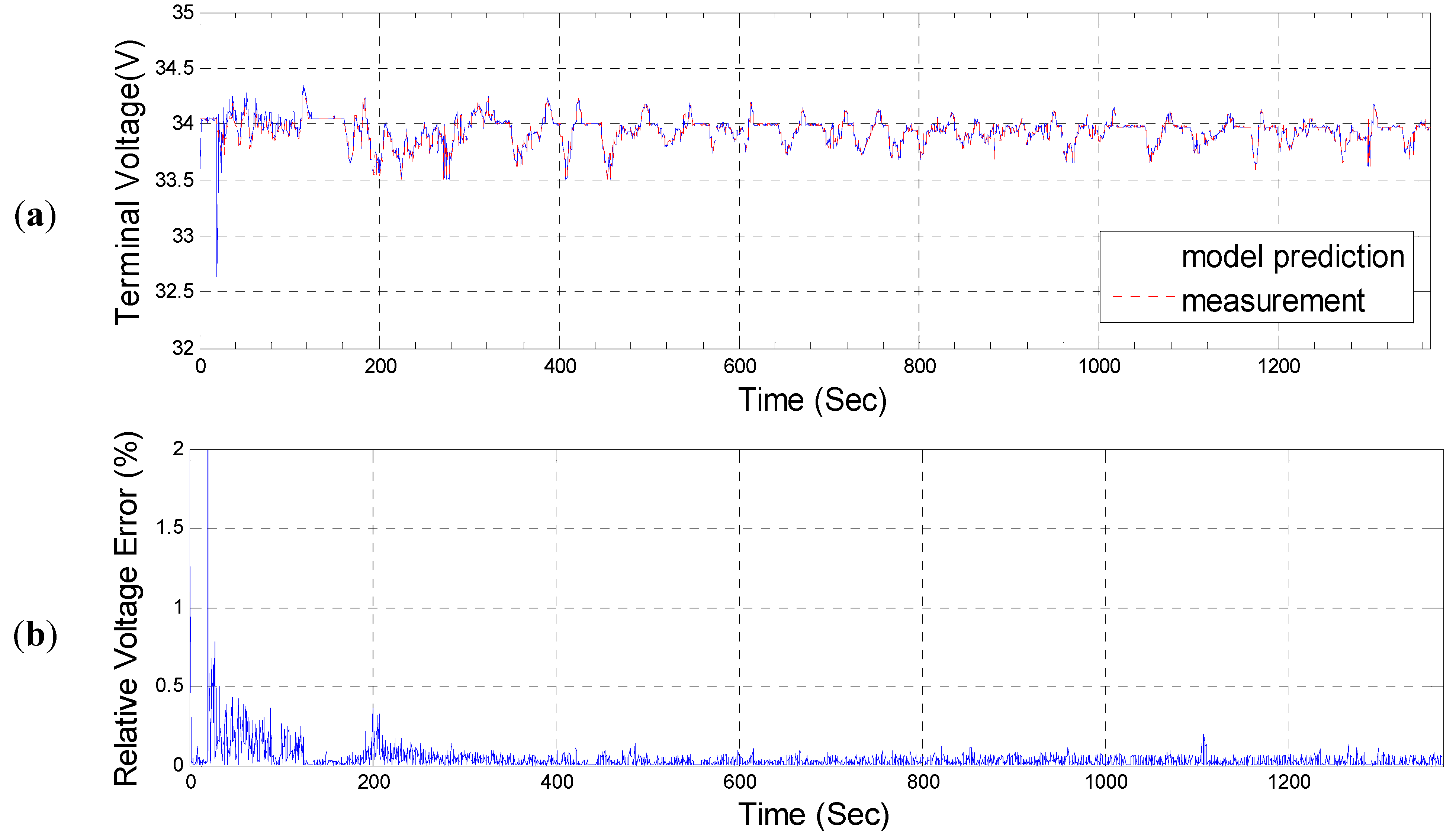
4.2. Experiments


5. Conclusions
Nomenclature:
| Cp | polarization capacitance |
| cj,m | scaling coefficient of wavelet MRA expansion |
| dj,m | wavelet coefficient of wavelet MRA expansion |
| f | any finite energy signal |
| gi | Haar wavelet basis function |
| h | battery state of charge |
| ib | battery outflow current |
| j | scale level of wavelet MRA expansion |
| j0 | the coarsest scale of wavelet MRA expansion |
| jmax | the finest scale of wavelet MRA expansion |
| J | the truncation scale of truncated wavelet MRA expansion |
| k | discrete time |
| N | length of input/output |
| Rp | polarization resistance |
| Rs | ohmic internal resistance |
| t | continuous time |
| Tc | sampling period |
| u | nonparametric component of PLBM |
| vb | battery terminal voltage |
| vc | polarization voltage |
| voc | open circuit voltage |
| x | observed value of battery terminal voltage |
| y | observed value of battery outflow current |
Greek Symbols
| ε | zero-mean white noise |
| ηi | the ith wavelet expansion coefficient of the nonparametric component of PLBM |
| θi | the ith parameter of the parametric component of PLBM |
| λ | penalty factor |
| ϕ | wavelet scaling function |
| ψ | wavelet mother function |
Acronyms
| CCD | cyclic coordinate descent |
| MRA | multiresolution analysis |
| OCV | open circuit voltage |
| PLBM | partially linear battery model |
| RLS | recursive least square |
| SoC | state of charge |
| SoH | state of health |
Acknowledgments
Conflict of Interest
References
- Newman, J.; Thomas, K.E.; Hafezi, H.; Wheeler, D.R. Modeling of lithium-ion batteries. J. Power Sources 2003, 119, 838–843. [Google Scholar] [CrossRef]
- Song, L.; Evans, J.W. Electrochemical-thermal model of lithium polymer batteries. J. Electrochem. Soc. 2000, 147, 2086–2095. [Google Scholar] [CrossRef]
- He, H.; Xiong, R.; Fan, J. Evaluation of lithium-ion battery equivalent circuit models for state of charge estimation by an experimental approach. Energies 2011, 4, 5825–5898. [Google Scholar]
- Chen, M.; Rincon-Mora, G.A. Accurate electrical battery model capable of predicting runtime and I-V performance. IEEE Trans. Energy Convers. 2006, 21, 504–511. [Google Scholar] [CrossRef]
- Sitterly, M.; Yin, G.; Wang, C. Enhanced identification of battery models for real-time battery management. IEEE Trans. Sustain. Energy 2011, 2, 300–308. [Google Scholar] [CrossRef]
- Zhang, C.P.; Jiang, J.C.; Zhang, W.G.; Suleiman, M.S. Estimation of state of charge of lithium-ion batteries used in HEV using robust extended Kalman filtering. Energies 2012, 5, 10981–11115. [Google Scholar]
- Sarvi, M.; Ghaffarzadeh, N. A wavelet network based model for Ni-Cd batteries. Int. J. Electrochem. Sci. 2012, 7, 10291–10302. [Google Scholar]
- Shen, Y. Adaptive online state-of-charge determination based on neuro-controller and neural network. Energy Convers. Manag. 2010, 51, 1093–1098. [Google Scholar] [CrossRef]
- Shen, W.; Chan, C.; Lo, E.; Chau, K. A new battery available capacity indicator for electric vehicles using neural network. Energy Convers. Manag. 2002, 43, 817–826. [Google Scholar] [CrossRef]
- Tsang, K.; Sun, L.; Chan, W. Identification and modelling of lithium ion battery. Energy Convers. Manag. 2010, 51, 2857–2862. [Google Scholar] [CrossRef]
- Bhangu, B.; Bentley, P.; Stone, D.; Bingham, C. Nonlinear observers for predicting state-of-charge and state-of-health of lead-acid batteries for hybrid-electric vehicles. IEEE Trans. Veh. Tech. 2005, 54, 783–794. [Google Scholar] [CrossRef]
- Engle, R.F.; Granger, C.W.J.; Rice, J.; Weiss, A. Semiparametric estimates of the relation between weather and electricity sales. J. Am. Stat. Assoc. 1986, 81, 310–320. [Google Scholar] [CrossRef]
- Zhang, T.; Wang, Q. Semiparametric partially linear regression models for functional data. J. Stat. Plan. Infer. 2012, 142, 2518–2529. [Google Scholar] [CrossRef]
- Chang, X.W.; Qu, L. Wavelet estimation of partially linear models. Comp.Stat. Data Anal. 2004, 47, 31–48. [Google Scholar] [CrossRef]
- Hu, X.; Sun, F.; Zou, Y.; Peng, H. Online Estimation of an Electric Vehicle Lithium-Ion Battery Using Recursive Least Squares with Forgetting. In Proceedings of the 2011 American Control Conference, San Francisco, CA, USA, 29 June–1 July 2011; pp. 935–940.
- Kim, I.S. The novel state of charge estimation method for lithium battery using sliding mode observer. J. Power Sources 2006, 163, 584–590. [Google Scholar] [CrossRef]
- Chiang, Y.H.; Sean, W.Y.; Ke, J.C. Online estimation of internal resistance and open-circuit voltage of lithium-ion batteries in electric vehicles. J. Power Sources 2011, 196, 3921–3932. [Google Scholar] [CrossRef]
- Hu, Y.; Yurkovich, S. Linear parameter varing battery model identification using subspace methods. J. Power Sources 2011, 196, 2913–2923. [Google Scholar] [CrossRef]
- Gould, C.; Bingham, C.; Stone, D.; Bentley, P. New battery model and state-of-health determination through subspace parameter estimation and state-observer techniques. IEEE Trans. Veh. Tech. 2009, 58, 3905–3916. [Google Scholar] [CrossRef] [Green Version]
- Zhang, C.P.; Zhang, C.N.; Liu, J.Z.; Sharkh, S.M. Identification of dynamic model parameters for lithium-ion batteries used in hybrid electric vehicles. High Technol. Lett. 2010, 16, 6–12. [Google Scholar] [CrossRef]
- He, H.; Xiong, R.; Guo, H. Online estimation of model parameters and state-of-charge of LiFePO4 batteries in electric vehicles. Appl. Energy 2012, 89, 413–420. [Google Scholar] [CrossRef]
- Fadili, J.M.; Bullmore, E. Penalized partially linear models using sparse representations with an application to fMRI time series. IEEE Trans. Signal Process. 2005, 53, 3436–3448. [Google Scholar] [CrossRef]
- Ding, H.; Claeskens, G.; Jansen, M. Variable selection in partially linear wavelet models. Statist. Model. 2011, 11, 409–427. [Google Scholar] [CrossRef]
- Espinoza, M.; Suykens, J.A.K.; de Moor, B. Kernel based partially linear models and nonlinear identification. IEEE Trans. Autom. Control 2005, 50, 1602–1606. [Google Scholar] [CrossRef]
- Yu, Y.; Ruppert, D. Penalized spline estimation for partially linear single-index models. J. Am. Stat. Assoc. 2002, 97, 1042–1054. [Google Scholar] [CrossRef]
- Donoho, D.L.; Johnstone, J.M. Ideal spatial adaptation by wavelet shrinkage. Biometrika 1994, 81, 425–455. [Google Scholar] [CrossRef]
- Meyer, F.G. Wavelet-based estimation of a semiparametric generalized linear model of fMRI time-series. IEEE Trans. Med. Imag. 2003, 22, 315–322. [Google Scholar] [CrossRef]
- Wu, T.T.; Lange, K. Coordinate descent algorithms for lasso penalized regression. Ann. Appl. Stat. 2008, 2, 224–244. [Google Scholar] [CrossRef]
- Friedman, J.; Hastie, T.; Höfling, H.; Tibshirani, R. Pathwise coordinate optimization. Ann. Appl. Stat. 2007, 1, 302–332. [Google Scholar] [CrossRef]
- Angelosante, D.; Bazerque, J.A.; Giannakis, G.B. Online adaptive estimation of sparse signals: Where RLS meets the l1-normal. IEEE Trans. Signal Process. 2010, 58, 3436–3447. [Google Scholar] [CrossRef]
- Kekatos, V.; Angelosante, D.; Giannakis, G.B. Sparsity-Aware Estimation of Nonlinear Volterra Kernels. In Proceedings of the 3rd IEEE International Workshop on Computational Advances in Multi-Sensor Adaptive Processing (CAMSAP), Aruba, Dutch Antilles, 13–16 December 2009; pp. 129–132.
- Pawlak, M.; Hasiewicz, Z. Nonlinear system identification by the Haar multiresolution analysis. IEEE Trans. Circuits Syst. I 1998, 45, 945–961. [Google Scholar] [CrossRef]
- Wei, H.; Billings, S. A unified wavelet-based modelling framework for non-linear system identification: The WANARX model structure. Int. J. Control 2004, 77, 351–366. [Google Scholar] [CrossRef]
- Billings, S.A.; Wei, H.L. A new class of wavelet networks for nonlinear system identification. IEEE Trans. Neural Netw. 2005, 16, 862–874. [Google Scholar] [CrossRef] [PubMed]
- Sliwinski, P.; Hasiewicz, Z. Computational algorithms for wavelet identification of nonlinearities in hammerstein systems with random inputs. IEEE Trans. Signal Process. 2008, 56, 846–851. [Google Scholar] [CrossRef]
© 2013 by the authors; licensee MDPI, Basel, Switzerland. This article is an open access article distributed under the terms and conditions of the Creative Commons Attribution license (http://creativecommons.org/licenses/by/3.0/).
Share and Cite
Mu, D.; Jiang, J.; Zhang, C. Online Semiparametric Identification of Lithium-Ion Batteries Using the Wavelet-Based Partially Linear Battery Model. Energies 2013, 6, 2583-2604. https://0-doi-org.brum.beds.ac.uk/10.3390/en6052583
Mu D, Jiang J, Zhang C. Online Semiparametric Identification of Lithium-Ion Batteries Using the Wavelet-Based Partially Linear Battery Model. Energies. 2013; 6(5):2583-2604. https://0-doi-org.brum.beds.ac.uk/10.3390/en6052583
Chicago/Turabian StyleMu, Dazhong, Jiuchun Jiang, and Caiping Zhang. 2013. "Online Semiparametric Identification of Lithium-Ion Batteries Using the Wavelet-Based Partially Linear Battery Model" Energies 6, no. 5: 2583-2604. https://0-doi-org.brum.beds.ac.uk/10.3390/en6052583