Quantitative Analysis of Lithium-Ion Battery Capacity Prediction via Adaptive Bathtub-Shaped Function

Abstract

Batteries are one of the most important components in many mechatronics systems, as they supply power to the systems and their failures may lead to reduced performance or even catastrophic results. Therefore, the prediction analysis of remaining useful life (RUL) of batteries is very important. This paper develops a quantitative approach for battery RUL prediction using an adaptive bathtub-shaped function (ABF). ABF has been utilised to model the normalised battery cycle capacity prognostic curves, which attempt to predict the remaining battery capacity with given historical test data. An artificial fish swarm algorithm method with a variable population size (AFSAVP) is employed as the optimiser for the parameter determination of the ABF curves, in which the fitness function is defined in the form of a coefficient of determination ($R^2$). A 4 × 2 cross-validation (CV) has been devised, and the results show that the method can work valuably for battery health management and battery life prediction.

1. Introduction

Estimating the remaining useful lifetime (RUL) of a lithium-ion battery is one of the most important requirements for mechatronics systems, such as portable devices, satellites, deep space probes, robotic systems and hybrid vehicles, in which prognostics and health management (PHM) technologies are used to assess the reliability and performance of a mechatronics product and, under its actual lifecycle conditions, to determine the advent of failure and mitigate system risk.

Much research on estimating the remaining useful life of batteries has been carried out in recent years (see [1,2,3,4,5,6,7,8] for examples). Ramadass et al. [1] developed a capacity fade prediction model of a semi-empirical approach for Li-ion cells, in which a diffusion coefficient of the Lithium electrode was taken as the accounting parameter for the rate capacity losses during cycling. Kozlowski et al. [2,3] discussed data fusion prognostic approaches of feature vectors, auto regressive moving average(ARMA), neural networks and fuzzy logic for the assessment of the state of charge (SOC), state of health (SOH) and state of life (SOL) of batteries. Goebel and Saha [4,5] presented a comparative study for the estimation of the RUL of batteries, in which the autoregressive integrated moving average (ARIMA), extended Kalman filtering (EKF), relevance vector machine (RVM) and particle filter (PF) are used. Burgess [6] proposed a method to assess the RUL of valve regulated lead-acid batteries using capacity measurements and Kalman filtering. He et al. [7] proposed an empirical model using Dempster-Shafer Theory (DST) and Bayesian Monte Carlo (BMC) for state of health (SOH) and RUL estimations with available battery data. Ecker et al. [8] proposed a parametrised semi-empirical ageing model for a multi-variable analysis of accelerated lifetime experiments of a hybrid electric vehicle under typical operating conditions.

The artificial fish swarm algorithm (AFSA) was first proposed in 2002 [9], inspired by the social behaviours of fish schools in searching, swarming and following. A schooling fish can quickly respond to the changes in the direction and speed of their neighbours; information about their behaviours has been passed to others, which help them move from one configuration to another, almost as one unit. By borrowing this intelligence of the social behaviours, the AFSA is parallel, independent of the initial values and able to achieve a global optimum.

In recent years, computational intelligence methods have been widely used in empirical applications [10,11,12,13,14,15,16,17,18,19], such as genetic algorithms (GA), swarm algorithms, fuzzy logic methods and artificial neural network (ANN). To increase predict efficiency and accuracy, researchers have tried to combine different algorithms to build hybrid approaches. In this paper, the AFSAVP is employed as the optimisation tool for the fast quantitative analysis of a battery residual capacity estimation using adaptive bathtub-shaped function (ABF)-based fitness function. Taking the advantages of the ABF’s highly flexible ability of parametric representation and the newly developed high efficient AFSA method with a variable population size (AFSAVP) [20,21].

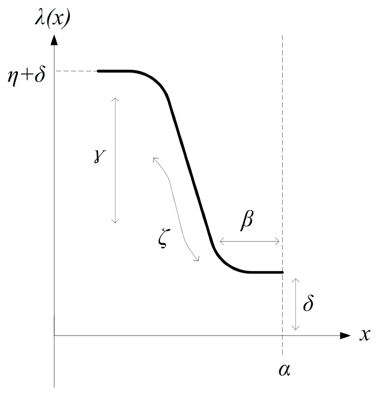
This paper is organised as follows. Section 1 introduces the background of the quantitative approach for battery remaining useful life and the artificial fish swarm algorithm method. Section 2 introduces the definition of the adaptive bathtub-shaped function. Section 3 describes the method of AFSAVP. Section 4 discusses the modelling of battery capacity prediction. Section 5 defines the fitness function of battery capacity prediction using an index of the mean average precious of the coefficient of determination. Section 6 discusses the parameter determination for the battery capacity prediction using the experimental data. In Section 7, the feasibility of the AFSAVP-driven battery capacity behaviours approach using the adaptive bathtub-shaped function is concluded.

2. Adaptive Bathtub-Shaped Functions

The ABF was first proposed by Chen [19] to provide a parametric representation of the failure behaviours for universal applications. The ABF has been employed for a complementary metal-oxide-semiconductor (CMOS) life data prediction [20]. In that case, a CMOS device acceleration test was devised, and the quantitative representation of the failure behaviours was well demonstrated, which indicates a flexible parametric performance of the ABF function with the given CMOS experimental data.

As demonstrated in Figure 1, the ABF, $\lambda \left(x\right)$, is defined in Equation (1), where α is the support factor, β is the boundary factor, γ is the internal scale factor, ζ is the shape factor, η is the external scale factor and δ is the shift factor [19,20].

$$\lambda \left(x\right)=\left\{\begin{array}{cc}\delta +\eta \left(1-e^{{\displaystyle -\frac{{\left(\left|x-\alpha \right|-\beta \right)}^{\zeta }}{\gamma }}}\right)\hfill & \mathrm{if}\left|\mathrm{x}-\alpha \right|\ge \beta ,\mathrm{x}\ge 0\hfill \\ & \\ \delta \hfill & \mathrm{if}\left|\mathrm{x}-\alpha \right|<\beta ,\mathrm{x}\ge 0\hfill \end{array}\right.$$

(1)

In the case of δ = 0 and η = 1, Equation (1) can be re-written as Equation (2), which is taken as the basic formula of the fitness function definition in Section 5.

Figure 1. The adaptive bathtub-shaped function [19].

Figure 1. The adaptive bathtub-shaped function [19].

$$\lambda \left(x\right)=\left\{\begin{array}{cc}1-e^{{\displaystyle -\frac{{\left(\left|x-\alpha \right|-\beta \right)}^{\zeta }}{\gamma }}}\hfill & \mathrm{if}\left|\mathrm{x}-\alpha \right|\ge \beta ,\mathrm{x}\ge 0\hfill \\ & \\ 0\hfill & \mathrm{if}\left|\mathrm{x}-\alpha \right|<\beta ,\mathrm{x}\ge 0\hfill \end{array}\right.$$

(2)

3. Swarm Fish Algorithm with Variable Population

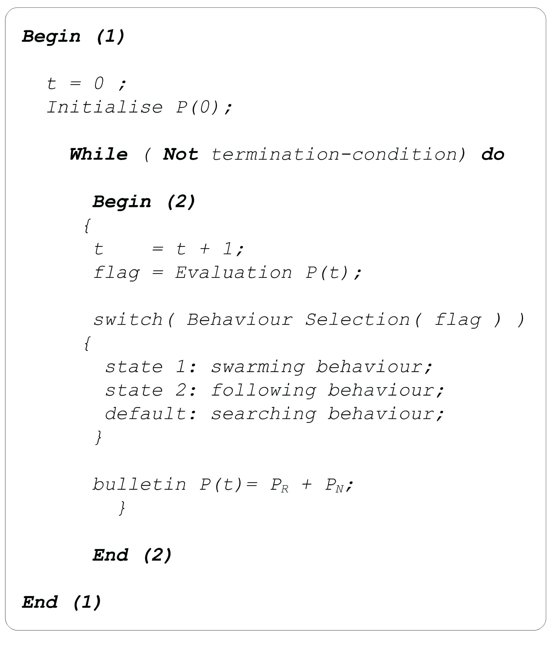
Inspired by the swarm intelligence of fish schooling behaviours, the AFSA is an artificial intelligent algorithm that simulates the behaviour of an individual artificial fish (AF) and then constructs an AF school. The AFSAVP flow chart in pseudocode is given in Figure 2; similar to the basic AFSA, the AFSAVP includes five steps of operations: (1) behaviour selection; (2) searching behaviour; (3) swarming behaviour; (4) following behaviour; and (5) bulletin and update.

Figure 2. The variable population size fish swarm algorithm pseudocode.

Figure 2. The variable population size fish swarm algorithm pseudocode.

Behaviour selection is to select one of the three types behaviours, i.e., searching, swarming and following, according to the parameters of the food density, the number of companion and visual conditions, in which the searching behaviour is taken as the default behaviour.

In the searching behaviour, one AF individual’s finite state set is defined as $S_k=\{s_1,\cdots ,s_M\}$, $k=1,\cdots ,M$; M is the total types of states. When the AF is in this behaviour, it moves from the current state, $S_i$ stated in Equation (3), to the next state, $S_j$, randomly and updates its state conditions, as stated in Equation (4), where ϝ is the food density for this AF, δ is the iterate step and υ is the AF visual constant:

$$S_{i+1}=\left\{\begin{array}{cc}{\displaystyle S_i+random·\delta ·\frac{S_j-S_i}{\parallel S_j-S_i\parallel }}\hfill & ,\mathrm{if}{ϝ}_j>{ϝ}_i\hfill \\ & \\ S_i+random·\delta \hfill & ,\mathrm{otherwise}\hfill \end{array}\right.$$

(3)

$$S_j=S_i+random·\upsilon$$

(4)

In the swarming behaviour, as stated in Equation (5), one AF is swarming with α neighbours within its visual field, in which $S_c$ is the central state, ${ϝ}_c$ is the food density and η is the crowd factor.

$$S_{i+1}=\left\{\begin{array}{cccc}{\displaystyle S_i+random·\delta ·\frac{S_c-S_i}{\parallel S_c-S_i\parallel }}\hfill & {\displaystyle ,\mathrm{if}\frac{{ϝ}_c}{\alpha }>\eta {ϝ}_i}\hfill & and\hfill & \eta \ge 1\hfill \\ & \\ Equation\left(3\right)\hfill & {\displaystyle ,\frac{{ϝ}_c}{\alpha }\le \eta {ϝ}_i}\hfill & or\hfill & \eta =0\hfill \end{array}\right.$$

(5)

In following behaviour, as stated in Equation (6), one AF updates its state under the condition of food density or moves to searching behaviour.

With the same conditions as Equation (5), the AF updates its state in the highest food density area; otherwise, the AF will go on with the searching behaviour, as expressed in Equation (5). With α AF neighbours around, when the food density reaches the “max” state ${ϝ}_{max}$, the AF’s companions gather to a upper limit.

$$S_{i+1}=\left\{\begin{array}{cccc}{\displaystyle S_i+random·\delta ·\frac{S_{max}-S_i}{\parallel S_{max}-S_i\parallel }}\hfill & {\displaystyle \mathrm{if}\frac{{ϝ}_{max}}{\alpha }>\eta {ϝ}_i}\hfill & and\hfill & \eta \ge 1\hfill \\ & \\ Equation\left(3\right)\hfill & {\displaystyle \frac{{ϝ}_{max}}{\alpha }\le \eta {ϝ}_i}\hfill & or\hfill & \eta =0\hfill \end{array}\right.$$

(6)

As described by Equation (7), the bulletin operation compares each AF’s current state with its historical state, which will be replaced and updated if the current state is better than the last one.

$$S_{j+1}=\left\{\begin{array}{cc}{S}_j\hfill & \mathrm{if}{ϝ}_j>{ϝ}_i\hfill \\ & \\ S_i\hfill & \mathrm{otherwise}\hfill \end{array}\right.$$

(7)

A “max-generation” is the trial number of an AF school searching for food under given initial conditions, which is one of the widely used criteria for terminating the AFSAVP simulation [21].

4. Battery Capacity Prediction

Table 1 summarises the batteries test conditions; in this test, the test batteries have a graphite anode and a lithium cobalt oxide cathode verified by electron dispersive spectroscopy, with a rated 0.9 $Ah$ capacity. The tests were accomplished by multiple charge-discharge cycles using an Arbin BT2000 battery test equipment under room temperature [7], and the discharge current was 0.45 A, the batteries’ charging and discharging cut-off voltage was 2.5 V, guided by the manufacturer’s specification, and the capacity of the tested batteries was assessed by the Coulomb counting method with full charge-discharge cycles.

Table 1. Summary of battery test conditions.

No.	Test equipment	Temperature	Cycles	Discharge current
A3	Arbin BT2000	20 ${}^{\circ }$C–25 ${}^{\circ }$C	300	0.45A
A5	Arbin BT2000	20 ${}^{\circ }$C–25 ${}^{\circ }$C	300	0.45A
A8	Arbin BT2000	20 ${}^{\circ }$C–25 ${}^{\circ }$C	300	0.45A
A12	Arbin BT2000	20 ${}^{\circ }$C–25 ${}^{\circ }$C	300	0.45A

Table 1. Summary of battery test conditions.

No.	Test equipment	Temperature	Cycles	Discharge current
A3	Arbin BT2000	20 ${}^{\circ }$C–25 ${}^{\circ }$C	300	0.45A
A5	Arbin BT2000	20 ${}^{\circ }$C–25 ${}^{\circ }$C	300	0.45A
A8	Arbin BT2000	20 ${}^{\circ }$C–25 ${}^{\circ }$C	300	0.45A
A12	Arbin BT2000	20 ${}^{\circ }$C–25 ${}^{\circ }$C	300	0.45A

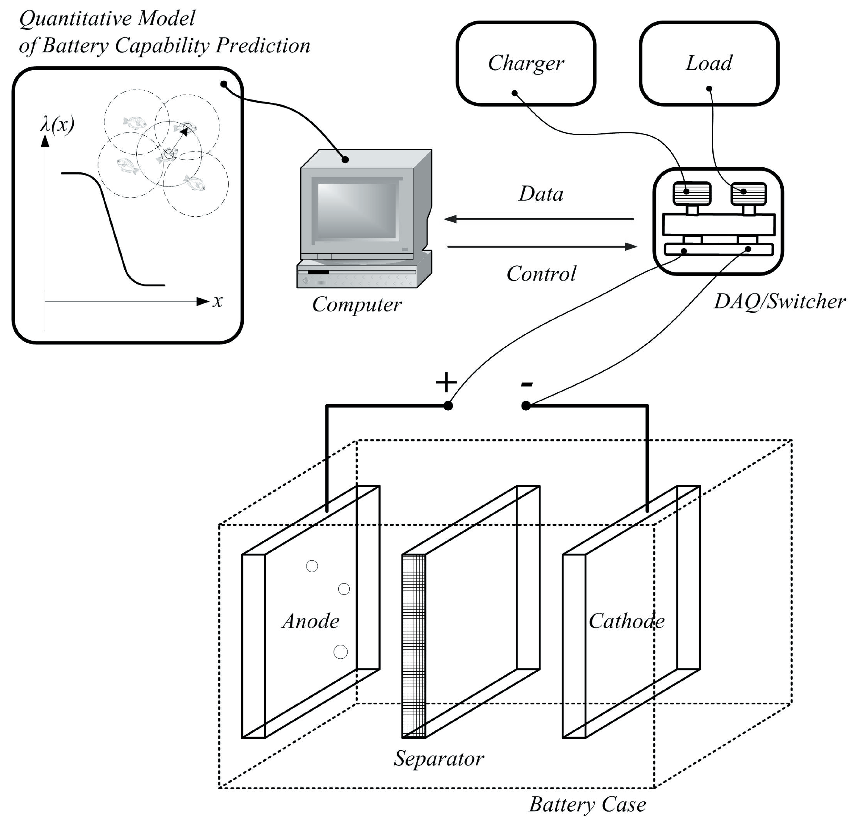
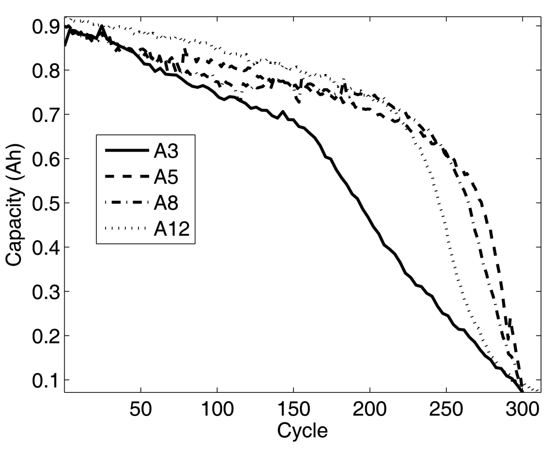
Figure 3 gives the battery capacity experimental setup, which consists of a set of Lithium-ion battery cases, chargers, loads, data acquisition (DAQ) system, switchers, a computer for control and analysis and some other modules, such as a set of sensors of voltage, current and temperature. As can be seen in Figure 4, there are four groups of the battery capacity raw data (observed data), A3, A5, A8 and A12.

Figure 3. Schematic of a battery capacity experiment setup.

Figure 3. Schematic of a battery capacity experiment setup.

Figure 4. Battery raw data: A3, A5, A8 and A12.

Figure 4. Battery raw data: A3, A5, A8 and A12.

Inspired by the shapes and trends of the raw data curves, the ABF is employed to build a parametric model for the experimental data based on prediction analysis.

Let’s define a vector, $X_j$, with the values, $\{x_1,x_2,...,x_i,...,x_n\}$, as the observed battery capacity data, a vector, ${\widehat{X}}_j$, with the values, $\{{\widehat{x}}_1,{\widehat{x}}_2,...,{\widehat{x}}_i,...{\widehat{x}}_n\}$, as the estimated battery capacity data, where i = $1,2,...,n$, j = $1,2,...,N$, n is the length of the vector, $X_j$, and the population of vectors, $X_j$, as 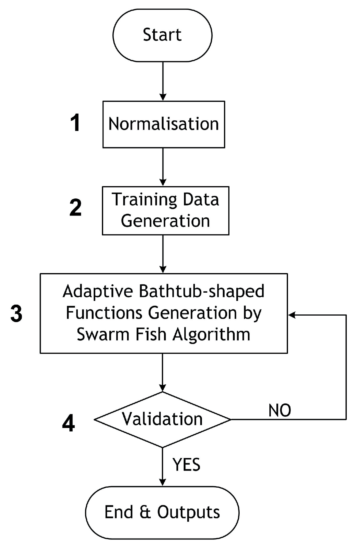N. The flow chart of the battery capacity prediction analysis is given in Figure 5, in which there are five steps, as described below,

Step 1—Normalisation: since the four groups of data are not the same length, all the raw data need to be normalised by scale and shift operations before the next step. The data shift and scale operations are stated in Equations (8) and (9), respectively [22]. The charge-discharge cycles (x-axis, unit: cycle) and the battery capacity (y-axis, unit: Ah) are put through the normalisation.

As given in Equation (8), the scale operation first calculates the scale factor according to the input range, $[x_{min},x_{max}]$, of the raw data, $x_i$, and then, all the input data are scaled to the range of $[c_l,c_u]$. That is, The variables are mapped from the practical value range, $[x_{min},x_{max}]$, to the normalised value range, $[c_l,c_u]$, which are $[0,1]$ in this context.

$${\displaystyle x_{i_c}=\left(c_u-c_l\right)\times \frac{x_i-x_{min}}{x_{max}-x_{min}}}$$

(8)

In the shift operation, the scaled data, $x_{i_c}$, are shifted to the unit range of $[c_l,c_u]$, as given in Equation (9).

$${\displaystyle x_{i_h}=c_l+x_{i_c}}$$

(9)

Step 2—Training data generation: there are four groups, $a_k$, for the training data generation. Each of the groups is calculated from the mean values of three out of the four raw data, A3, A5, A8 and A12, as stated in Equation (10). Table 2 lists the raw data grouping for each training data generation. The validation data are $b_k$.

$${\displaystyle T_k=\frac{a_k}{3}}$$

(10)

Figure 5. Battery capacity prediction flow chart.

Figure 5. Battery capacity prediction flow chart.

Table 2. Data grouping for training and validation capacity (Ah).

j	Training samples ${\mathit{a}}_{\mathit{j}}$	Validation samples ${\mathit{b}}_{\mathit{j}}$
1	A3 + A5 + A8	A12
2	A3 + A5 + A12	A8
3	A3 + A8 + A12	A5
4	A5 + A8 + A12	A3

Table 2. Data grouping for training and validation capacity (Ah).

j	Training samples ${\mathit{a}}_{\mathit{j}}$	Validation samples ${\mathit{b}}_{\mathit{j}}$
1	A3 + A5 + A8	A12
2	A3 + A5 + A12	A8
3	A3 + A8 + A12	A5
4	A5 + A8 + A12	A3

Step 3—ABF generation and optimisation: as defined in Equation (1), the ABF, $\lambda \left(x\right)$, was employed to approximate the experimental data by the predicted data, ${\widehat{x}}_i$, in which four parameters (α, β, ζ and γ) of ABF need to be determined by the AFSAVP.

Step 4—Validation and error analysis: the errors analysis of the estimated battery capacity data, ${\widehat{x}}_i$, and experimental data, $x_i$, validates the optimisation process.

5. Fitness Function

In this section, an index of the mean average precious (mAP) of the coefficient of determination ($R^2$) is defined as the fitness to evaluate the optimisation process.

As given in Equation (11), $R^2$ is a quantity utilised to measure the proportion of total fluctuation in the response trend prediction analysis, and a larger $R^2$ indicates a closer similarity between the predicted data, ${\widehat{x}}_i$, and the experimental data, $x_i$ [23,24]. ${\overline{x}}_i$ is the mean value of the observed data, $x_i$.

$$R_j^2\left(x_i,{\widehat{x}}_i\right)={\left(1-\frac{{\displaystyle \sum _{i=1}^n}{\left(x_i-{\widehat{x}}_i\right)}^2}{{\displaystyle \sum _{i=1}^n}{\left(x_i-{\overline{x}}_i\right)}^2}\right)}_{{|}_{X_j}}$$

(11)

The mAP is the mean of the average precision scores for each vector, $X_j$, as expressed in Equation (12), in which N is the population of the data set and Avg$\left(*\right)$ is the average value of each data sequence.

$$\mathrm{mAP}\left(X_j\right)=\frac{{\displaystyle \sum _{j=1}^N}\mathrm{Avg}\left(X_j\right)}{N}$$

(12)

The fitness function, F, of battery capacity prediction is given in Equation (13).

$$F=\mathrm{mAP}\left(R_j^2\left(x_i,{\widehat{x}}_i\right)\right)$$

(13)

6. Simulation Results and Discussions

The simulation results for the AFSAVP-driven hybrid modelling of the battery capacity behaviours are performed by $SwarmFish$, which is a toolbox for MATLAB developed by Chen [25]. According to previous research and engineering applications, the parameters for the battery capacity prediction are initialised in Table 3, in which a max generation of 100 is the termination condition of each round test; the total test number is 100; the visual factor is 2.5; the crowd factor is 0.618; the population is 30, in which the non-replaceable, $P_N$, and replaceable population, $P_R$, are 20 and 10, respectively; the try number is five [19,20]; and the ranges of α, β, γ and ζ are [−10,10], [−10,10], [300,500] and [1,6], respectively.

Table 3. Parameters of the SwarmFish optimisation.

Parameter	Description	Value
	max generations	100
	test number	100
	visual factor	2.5
	crowd factor	0.618
	population	30
	try number	5
α	support factor	[−10,10]
β	boundary factor	[−10,10]
γ	internal scale factor	[300,500]
ζ	shape factor	[1,6]

Table 3. Parameters of the SwarmFish optimisation.

Parameter	Description	Value
	max generations	100
	test number	100
	visual factor	2.5
	crowd factor	0.618
	population	30
	try number	5
α	support factor	[−10,10]
β	boundary factor	[−10,10]
γ	internal scale factor	[300,500]
ζ	shape factor	[1,6]

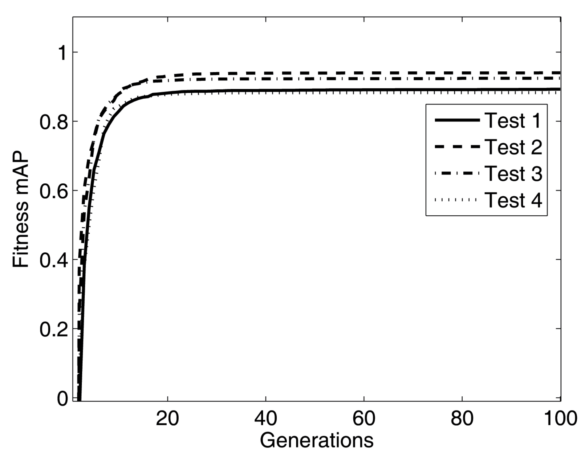
As can be observed in Figure 6, the fitness mAP curves of four tests are represented by four types of lines, in which the fitness curves go up very quickly from generation one to 20 to reach a plateau point (about generation 20). Then from generation 20 to 100, the curves keep steady over the rest of the generations and the fitness mAP moves to the convergence.

Figure 6. Fitness mAP of test 1, 2, 3 and 4.

Figure 6. Fitness mAP of test 1, 2, 3 and 4.

The 4 × 2 cross-validation (CV) is designed to validate the prediction method, in which the experimental data, A3, A5, A8 and A12, are split into two parts, one for training (training samples) and the other for validation (validation sample), as listed in Table 2.

Table 4 is the 4 × 2 CV comparison of the four tests with the four groups of data sets for battery capacity prediction in the [0,0.9] normalised cycle range. The mean and standard deviation (MEAN ± STD) of α, β, ζ and γ of the four tests are listed, which indicate the optimised locations of the parameter settings within their initial ranges. $error$ is the absolute error of the normalised battery capacity, between the predicted data and the experimental data of validation. The index of $error$ demonstrates the acceptable errors of the battery capacity prediction using ABF over the optimisation process, in which the $error$ values of the training tests are a little larger than the values of validation. The optimisation processes of Test 1 to Test 4 are demonstrated in Figure 7, Figure 8, Figure 9 and Figure 10, respectively.

As can be observed in Table 4, the different raw data sizes could cause different prediction errors. The mean of validation errors are 8.51% > 8.04% > 7.42% > 5.45%, which indicates the closer the data lengths, the errors of battery capacity prediction could be smaller. Also, as shown in Figure 4, the larger data size provides the better battery capacity prediction results. That is, if the given raw data scale is closer to real battery life time scale, the prediction result is better. Contrarily, small data scale and data size should result in poor predictions.

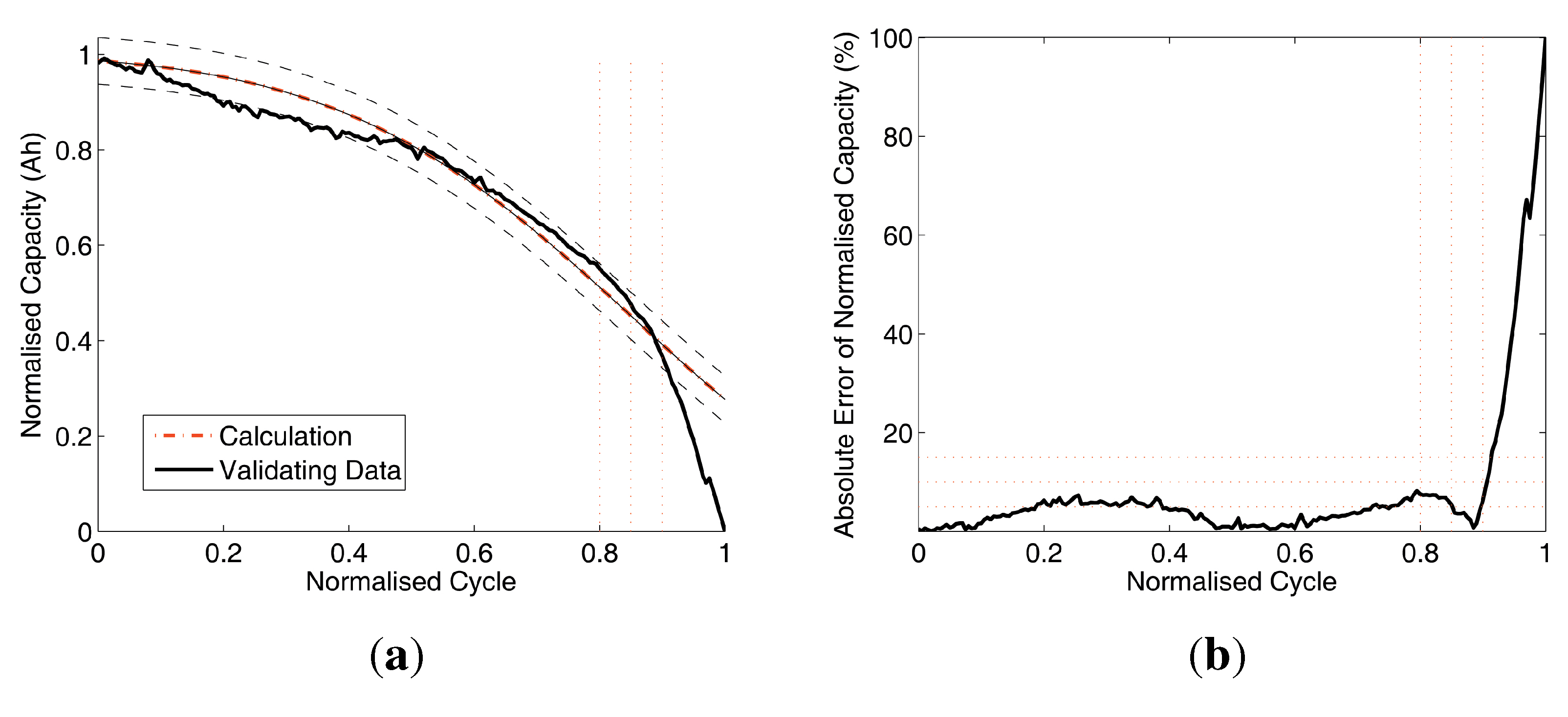
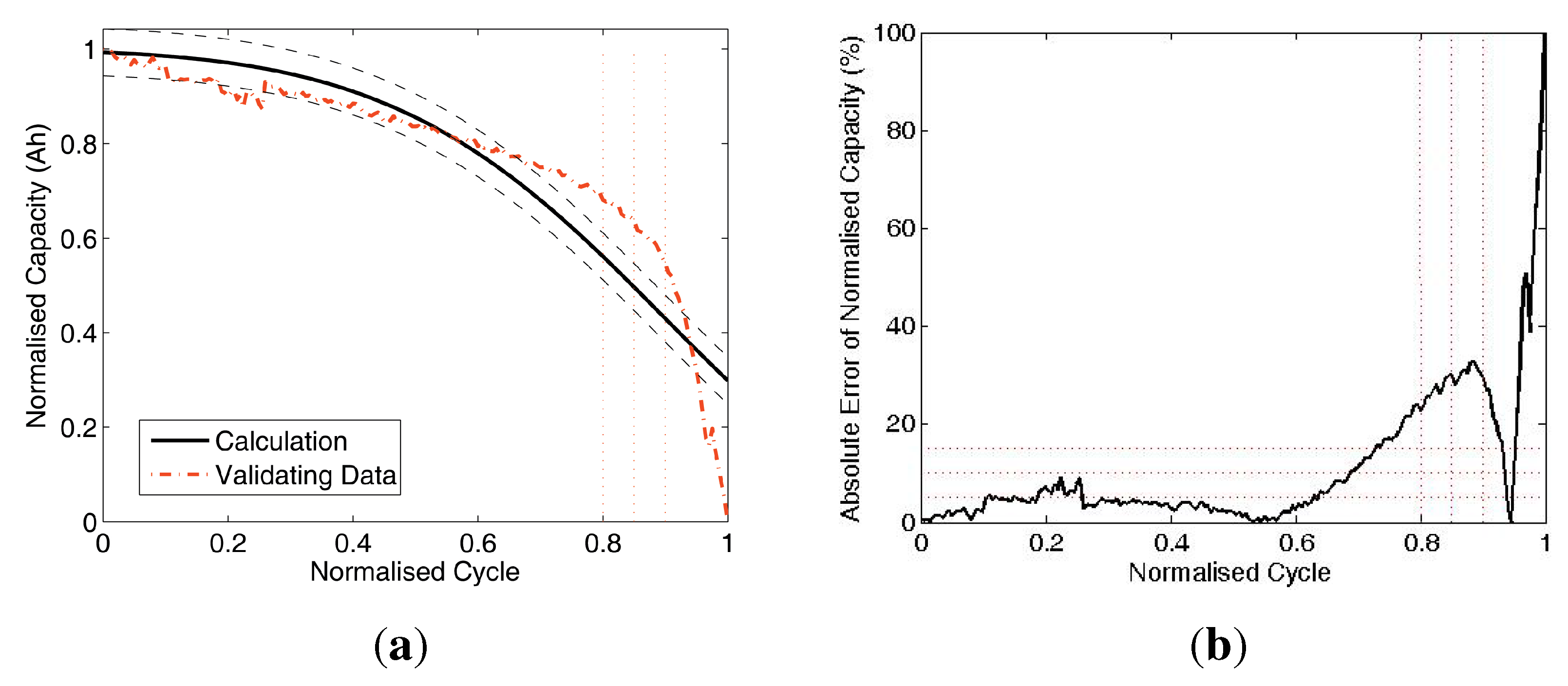
Figure 7, Figure 8, Figure 9 and Figure 10 are the plots for Test 1 to Test 4. There are two subfigures, (a) and (b), in Figure 7, Figure 8, Figure 9 and Figure 10. The calculation curves in subfigure (a) of Figure 7, Figure 8, Figure 9 and Figure 10 demonstrate the approximation curves of differences and similarity for Test 1 to Test 4 over the predicting process driven by the AFSAVP, which can be employed as the indicators of the battery capacity prediction.

Figure 7. Data comparison of Test 1. (a) Battery capacity prediction by training (A3,A5,A8) and validating (A12); (b) absolute errors of battery capacity prediction.

Figure 7. Data comparison of Test 1. (a) Battery capacity prediction by training (A3,A5,A8) and validating (A12); (b) absolute errors of battery capacity prediction.

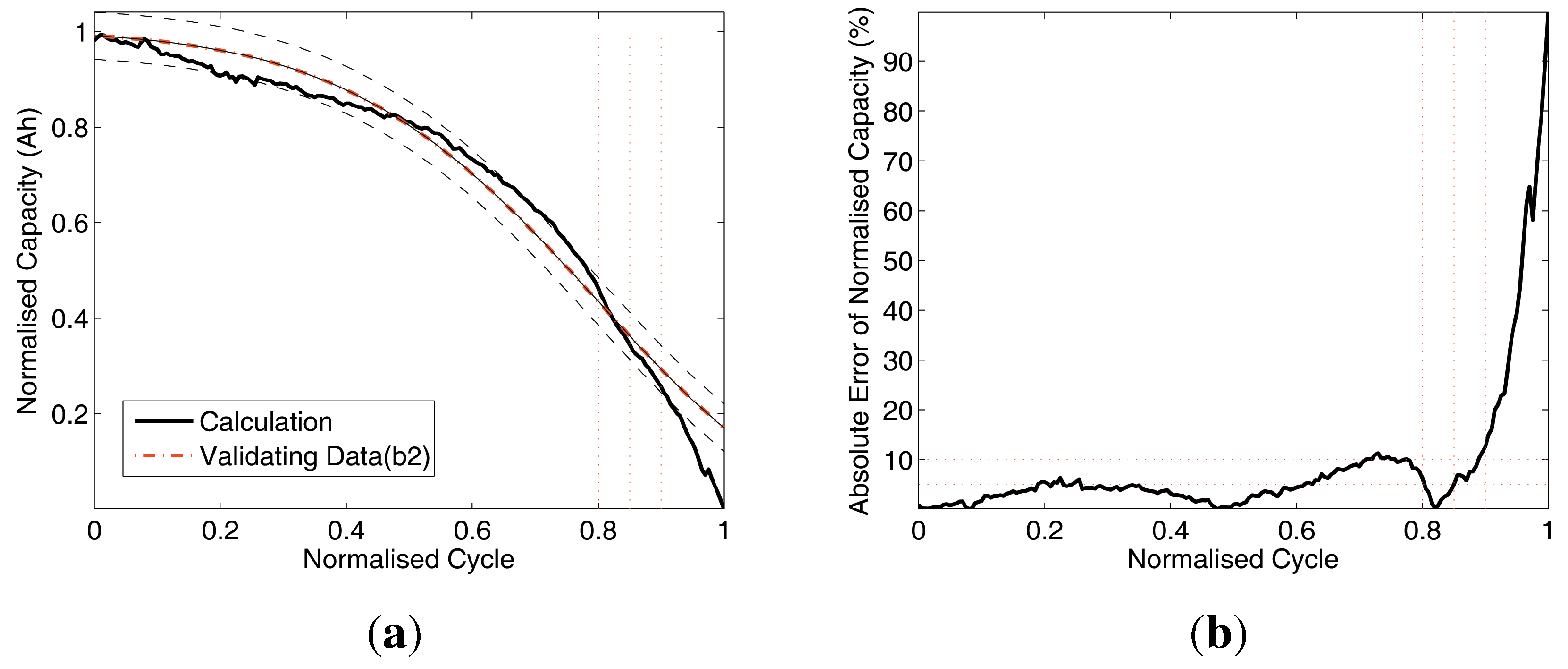
Figure 8. Data comparison of Test 2. (a) Battery capacity prediction by training (A3,A5,A12) and validating (A8); (b) absolute errors of battery capacity prediction.

Figure 8. Data comparison of Test 2. (a) Battery capacity prediction by training (A3,A5,A12) and validating (A8); (b) absolute errors of battery capacity prediction.

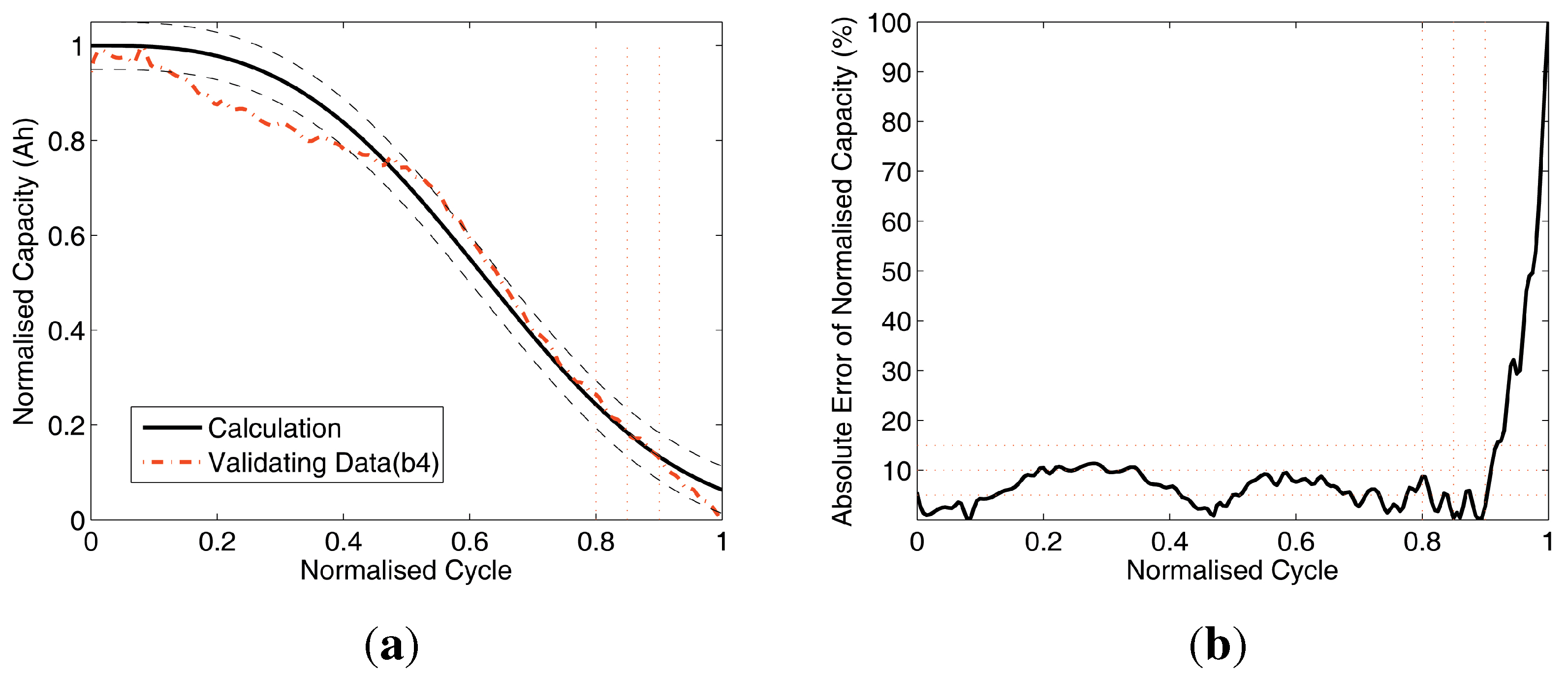
Figure 7(a), Figure 8(a), Figure 9(a) and Figure 10(a) compare the results with two curves: the validating ($b_j$, dash-dot line) and the calculated battery prediction data (solid line). Also, there are two dashed curves: the ±5% error upper and lower boundaries of the calculation curve, and there are three vertical dotted lines located at normalised cycle = 0.8, 0.85 and 0.9 as reference lines on the s-axis. Without losing significance, the normalised cycle range [0,.0.9] for the analysis is chopped from the full range of [0,1] to avoid the numerical singularity at normalised cycle = 1 and the errors closely caused by the singularity in the range of [0.9, 1]. Furthermore, there are three horizontal dotted reference lines at 5%, 10% and 15% on the y-axis.

Figure 9. Data comparison of Test 3. (a) Battery capacity prediction by training (A3,A8,A12) and validating (A5); (b) absolute errors of battery capacity prediction.

Figure 9. Data comparison of Test 3. (a) Battery capacity prediction by training (A3,A8,A12) and validating (A5); (b) absolute errors of battery capacity prediction.

Figure 10. Data comparison of Test 4. (a) Prediction and validating; (b) absolute errors of prediction.

Figure 10. Data comparison of Test 4. (a) Prediction and validating; (b) absolute errors of prediction.

The Subfigures (b) of Figure 7, Figure 8, Figure 9 and Figure 10 compare the absolute errors of validation. As shown in Figure 7, Figure 8, Figure 9 and Figure 10, subfigures (b) and Table 4, the mean errors (MEAN) are less than 10%, which indicate that this battery capacity prediction method is with acceptable accuracy for practical cases. The results also indicate that the proposed method can handle the raw data with different sizes, which is robust and applicable for field data acquisition system.

To summarise, the results indicate that the developed ABF-based prediction method can be employed to estimate the lithium-ion battery capacity and as a quantitative indicator to assist the users in their real-time applications.

Table 4. The 4 × 2 cross validation of battery capacity prediction (mean and standard deviation (MEAN ± STD)), (Ah).

NO.	Test 1		Test 2		Test 3		Test 4
	Training	Validation	Training	Validation	Training	Validation	Training	Validation
Datasets	(A3,A5,A8)	A12	(A3,A5,A12)	A8	(A3,A8,A12)	A5	(A5,A8,A12)	A3
α	0.97 ± 0.32		0.62 ± 0.91		0.72 ± 0.37		0.58 ± 0.04
β	0.39 ± 0.11		0.47 ± 0.82		0.58 ± 0.33		0.33 ± 0.93
γ	712.72 ± 47.23		515.43 ± 25.22		467.81 ± 84.52		500.75 ± 64.09
ζ	4.38 ± 0.53		4.62 ± 0.38		4.55 ± 0.35		4.68 ± 0.37
$e_A{|}_{max}$	2.8571%	5.9428%	3.7143%	3.4286%	8.5714%	1.1429%	4.0973%	15.1429%
RMS	0.0937	0.1219	0.0621	0.1486	0.0724	0.1452	0.0836	0.1757

Table 4. The 4 × 2 cross validation of battery capacity prediction (mean and standard deviation (MEAN ± STD)), (Ah).

NO.	Test 1		Test 2		Test 3		Test 4
	Training	Validation	Training	Validation	Training	Validation	Training	Validation
Datasets	(A3,A5,A8)	A12	(A3,A5,A12)	A8	(A3,A8,A12)	A5	(A5,A8,A12)	A3
α	0.97 ± 0.32		0.62 ± 0.91		0.72 ± 0.37		0.58 ± 0.04
β	0.39 ± 0.11		0.47 ± 0.82		0.58 ± 0.33		0.33 ± 0.93
γ	712.72 ± 47.23		515.43 ± 25.22		467.81 ± 84.52		500.75 ± 64.09
ζ	4.38 ± 0.53		4.62 ± 0.38		4.55 ± 0.35		4.68 ± 0.37
$e_A{|}_{max}$	2.8571%	5.9428%	3.7143%	3.4286%	8.5714%	1.1429%	4.0973%	15.1429%
RMS	0.0937	0.1219	0.0621	0.1486	0.0724	0.1452	0.0836	0.1757

7. Conclusions and Future Work

In this paper, a newly developed AFSAVP was employed to quantitatively predict battery RUL based on four groups of historical test data. Designed in the form of ABF, the index of mAP has been introduced as the fitness function of $R^2$ of observed battery data and estimated battery data for the optimisation process. The 4 × 2 cross-validation has been deployed to validate the developed model. Under this approach of battery capacity prediction, the four tests have shown agreement with the experiment results.

Quantitative analysis is always utilised to aid the users in the power sources planning to take good advantage of the available statistical battery data. The ABF formed a prognostic model that can capture the dynamic behaviours of the battery capacity. The contributions of this paper includes consideration of the dynamic behaviours of historical battery capacity, the development of a quantitative prediction analysis and a clear indicator of normalised battery capacity of the battery RUL for decision-making.

In aiming at on-board battery RUL prediction, this added-value approach has potential applications in the protection of battery failure for robotic systems (e.g., exoskeleton, robotic space tethers, humanoid robot and industrial robotics), mobile devices and other systems with electrochemical power sources. In further work, the frameworks of the computational intelligence aided design (CIAD) and computational intelligence aided engineering (CIAE) will be studied, and more computational intelligence (CI) methods, such as genetic algorithms, fuzzy logic method, artificial neural network and swarm algorithms, will be integrated into these frameworks for the recommended solutions of both an optimisation process and a decision process [14,18]. Some environmental factors, such as the ambient temperature, electricity usage per day, autonomy days and depth of discharge limit, should be considered for improved models. Furthermore, accelerated life test (ALT) techniques and small sample methodologies should also be employed to reduce the cost of battery capacity experiments.