GASP: Genetic Algorithms for Service Placement in Fog Computing Systems


Department of Engineering “Enzo Ferrari”, University of Modena and Reggio Emilia, Via P. Vivarelli 10/1, 41125 Modena, Italy
*
Author to whom correspondence should be addressed.
Algorithms 2019, 12(10), 201; https://0-doi-org.brum.beds.ac.uk/10.3390/a12100201
Submission received: 23 July 2019
/
Revised: 11 September 2019
/
Accepted: 18 September 2019
/
Published: 21 September 2019
Abstract
:Fog computing is becoming popular as a solution to support applications based on geographically distributed sensors that produce huge volumes of data to be processed and filtered with response time constraints. In this scenario, typical of a smart city environment, the traditional cloud paradigm with few powerful data centers located far away from the sources of data becomes inadequate. The fog computing paradigm, which provides a distributed infrastructure of nodes placed close to the data sources, represents a better solution to perform filtering, aggregation, and preprocessing of incoming data streams reducing the experienced latency and increasing the overall scalability. However, many issues still exist regarding the efficient management of a fog computing architecture, such as the distribution of data streams coming from sensors over the fog nodes to minimize the experienced latency. The contribution of this paper is two-fold. First, we present an optimization model for the problem of mapping data streams over fog nodes, considering not only the current load of the fog nodes, but also the communication latency between sensors and fog nodes. Second, to address the complexity of the problem, we present a scalable heuristic based on genetic algorithms. We carried out a set of experiments based on a realistic smart city scenario: the results show how the performance of the proposed heuristic is comparable with the one achieved through the solution of the optimization problem. Then, we carried out a comparison among different genetic evolution strategies and operators that identify the uniform crossover as the best option. Finally, we perform a wide sensitivity analysis to show the stability of the heuristic performance with respect to its main parameters.
1. Introduction
In the last few years, we have witnessed an ever increasing popularity of sensing applications, characterized by the fact that geographically distributed sensors produce huge amounts of data that are then pushed towards the Internet core where cloud computing data centers are located to be processed. However, this traditional approach may cause excessive delays for those applications and services that require data to be processed with very low and predictable latency, such as those related to systems for smart traffic monitoring, support for autonomous driving, smart grid, or fast mobility applications (i.e., smart connected vehicle or connected rails). Another important observation is that not all the data needs to go to the cloud data centers, but in many cases data could be preprocessed, aggregated, and filtered to store in the network core only a reduced meaningful set of data, thus avoiding unnecessarily stressing the network infrastructure.
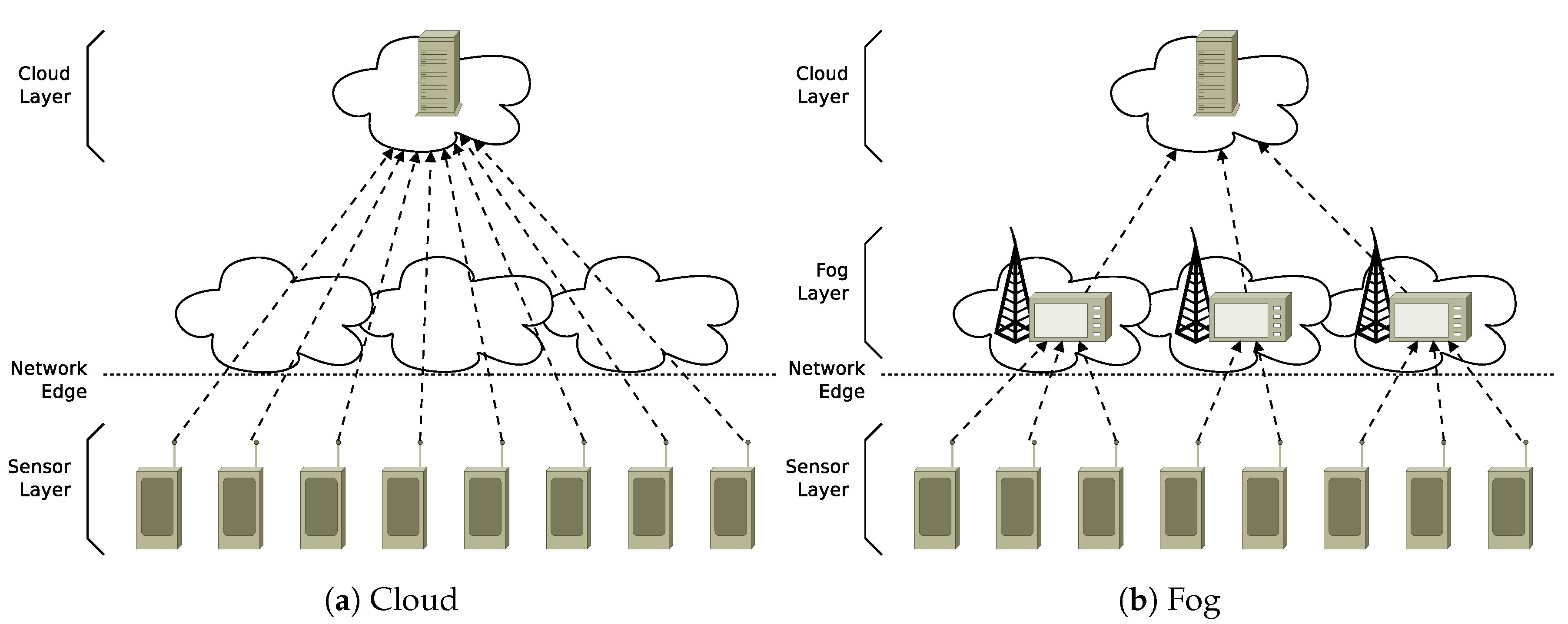
The emerging paradigm of fog computing represents a solution that can improve scalability and reduce application latency by extending cloud computing towards the edge of network [1,2]. Although in the traditional cloud architecture (Figure 1a) the data flows are sent directly from the “sensor layer” to the data center(s) in the “cloud layer”; in the fog infrastructure (Figure 1b), tasks and services may be moved close to the sources of data to be processed thanks to the presence of an intermediate layer of fog nodes, located at the network edge interposed between the cloud data center(s) and the sources of data. The innovative paradigm of fog computing is promising in addressing the still unsolved issues of cloud computing related to unreliable latency, lack of mobility support, and location-awareness. However, realizing the full potential of fog computing introduces several new challenges [3,4]. Many existing papers focus on balancing the load distribution between fog and cloud resources: among them, we should mentions the studies in the works by the authors of [5,6] that tackle the issue of optimizing the allocation of the processing tasks coming from the fog nodes over the cloud infrastructure. To this aim, different solutions are proposed, such as the possibility to rely on horizontal communication among fog nodes to reduce the service delay through load sharing mechanism.
On the other hand, less attention was received by the lower level connecting the data sources to the fog nodes. In the literature, indeed, many studies rely on the assumption that fog nodes communicate directly with sensors or mobile users through single-hop wireless connections [5] or that a domain of sensor nodes communicate with a specific and application-defined domain of fog nodes [6]. However, the choice of the fog node that receives and processes the data flow originated by a specific sensor may significantly affect the perceived latency and the overall performance of the application. Therefore, we claim that mapping the data flows from the sensors over the available fog nodes for processing and filtering tasks represents a critical issue to guarantee a high QoS in terms of latency and/or response time.
The contribution of this paper is two-fold:
- We present an optimization model for mapping the incoming data flows (sensor workload) over the nodes of the fog layer: the proposed model considers not only the processing time on the fog nodes depending on the local load, but also the latency between sensors and fog nodes due to the communication delay of the geographically distributed infrastructure.
- We propose an heuristic to provide a scalable solution to the problem of mapping sensors over fog nodes that could be applied to large-scale instances. The proposed heuristic is based on Genetic Algorithms (GAs), a method for solving both constrained and unconstrained optimization problems that relies on the natural selection process that drives biological evolution: those kind of algorithms have been previously, and successfully, exploited in the context of cloud computing and Software-as-a-Service placement [7]; but, to the best of our knowledge, it has never applied to fog computing infrastructures.
This paper extends a previous study by the same authors [8], representing a clear step ahead for the following reasons;
- the proposal of a more streamlined model for the optimization problem,
- a in-depth discussion of the genetic algorithm features and of their adaptation to the specific context,
- a new and more significant experimental setup, and
- new experimental results including a broad sensitivity analysis on the main heuristic parameters.
To evaluate the performance of the proposed solution, we consider a realistic smart city scenario as an example of a typical sensing environment where geographically distributed sensors produce data flows that require efficient processing for a wide range of possible applications, such as traffic monitoring and control, support for autonomous driving, and environmental sensing. Experiments were carried out on a geographic testbed representing a fog architecture whose nodes are realistically placed in the streets of a small-sized city (~180,000 inhabitants) in Emilia Romagna, Italy. The experiments show that the proposed heuristic can achieve performance similar to the one of a commercial solver applied to an optimization problem for mapping the data flows over the fog nodes. Then, we compare different genetic evolution strategies and operators to identify the best options (for example, we show how the uniform crossover outperforms other crossover operator or we demonstrate that the tournament selection is a better choice than the roulette selection). Finally, we evaluate the stability of the heuristic performance with respect to parameters, such as the number of generations, the probability of mutation and crossover, and the population size.
The remainder of this paper is organized as follows. Section 2 describes the problem formally and defines the considered optimization model, and Section 3 presents the heuristic algorithms proposed for solving the problem. Section 4 describes the experimental testbed and the results used to prove the viability of our approach. Finally, Section 5 discusses the related work and Section 6, concludes the paper with some final remarks, and outlines open research problems.
2. Problem Definition
This section describes the fog infrastructure and the problem of efficiently mapping the data flows coming from the sensors over the available fog nodes. In the second part of the section, we present the optimization model that formalized the mapping problem.
2.1. Mapping Problem
Our problem concerns the management of data flows in a fog infrastructure such as the one shown in Figure 1b. The infrastructure, which we assume to be deployed in a smart city scenario, is composed of three layers: a sensor layer, which produces data (represented as a set of wireless sensors at the bottom of the figure); a fog layer, which is responsible for a preliminary processing of data from the sensors (second layer in the figure); and a cloud layer, which is the final destination of the data (at the top of the figure). The underlying application logic involves the typical services of a smart city scenario. Sensors collect information about the city status, such as traffic intensity or air quality [9]. Such data should be collected at the level of a Cloud infrastructure to provide value-added services such as traffic or pollution forecast. The proposed fog layer intermediates the communication between the sensors and the cloud to provide scalability and reliability in the smart city services.
In our model, we assume a stationary scenario, where a set of similar sensors, , are distributed over an area (we consider the sensors to be not moving; although, a different scenario, where mobility is taken into account, can be easily introduced in our model). Furthermore, we assume that sensors are producing data at a steady rate, with a frequency that we denote as for the generic sensor i (for a summary of the symbols used in the model, the reader may refer to Table 1). The fog layer comprises a set of nodes that receive data from the sensors and perform operations on them. These operations typically include preprocessing of the data, such as filtering and/or aggregation, or may include some form of analysis to identify anomalies or problems as fast as possible. The refined data samples from the fog nodes are then sent to a cloud platform where additional analysis is carried out and where all the information is stored. These additional analysis tasks are typically highly expensive from a computational point of view.
As the problem concerning the management of large cloud data centers has been widely addressed in the literature [10,11], we do not consider the inner details of the cloud layer in our problem modeling, such as the computation time at the level of the cloud data center. Similarly, we do not consider the network-based latency due to the communication between the fog nodes and the cloud data center, as we assume this latency to be the same for all fog nodes and hence having no impact on the optimum mapping solution. Instead, we focus our attention to the problem of coordinating the communication of the elements in the sensor layer with the nodes in the fog layer. Specifically, we want to guarantee a high QoS, in terms of fast response. To this aim, we model the response time according to a queuing theory-based formulation, considering that the response time has two major contributions that should be taken into account:
- Network-based latency due to the communication between the sensor and the fog nodes. We denote this value as , where i is a sensor and j is a fog node.
- Computation time on the fog node. According to queuing theory, this time depends on the computation cost of the request (we denote as the time to process a packet of data from a sensor on fog node j, relying on the typical queuing theory notation) and on the rate, , of the jobs incoming at fog node j, where the value of is the sum of all the outgoing data rates, , of all the sensors, i, that are communicating with the fog node j.
For the sake of clarity we summarize the symbols used throughout the paper in Table 1.
2.2. Optimization Model
The main problem in the considered fog scenario is how to map on the fog nodes the data flows coming from the sensors. To this aim, we define an optimization problem where we use as the main decision variable a matrix of Boolean flags, . In our model, if and only if sensor i is sending data to fog node j; otherwise, . As the function of fog nodes is to preprocess the incoming data performing filtering and aggregation, we consider that all the data of a sensor must be sent to the same fog node and cannot be distributed across the fog layer.
Again, the reader may refer to Table 1 for a summary of the parameters used in our model.
The optimization model to address the previously-described problem can be formalized as follows, with an approach similar to the problem of allocating requests over a distributed infrastructure, such as VMs on a cloud [10,12,13]. In particular, we introduce a matrix of Boolean decision variables that is used to define the objective function and the constraints as follows,
subject to
In the problem formalization, objective function (1) aims to reduce the total (and hence the average) latency and processing time from every sensor to the fog computing nodes. The expression of response time used for our objective function is consistent with other studies in literature focusing on distributed cloud infrastructures [14]. Specifically, the average processing time is derived from Little’s result applied to a M/G/1 model and considers just the average arrival frequency and the processing rate of each fog node j. This definition of the response time has been widely adopted in literature, for example in [14]. The second part of the objective function, that is, the latency contribution, effectively captures the communication delay of a geographically distributed infrastructure using the latency .
Together with the objective function, we have a set of constraints. Equation (2) defines the incoming load, , on each fog node, j. Constraint (3) means that for every sensor, i, we direct its output to one and only one fog node. Constraint (4) guarantees that, for every fog node j, we avoid a congestion situation, where the incoming load exceeds the processing capability of that node. Finally, constraint (5) defines the Boolean nature of the decision variables .
3. Heuristic Algorithm
The optimization problem defined in the previous section aims to map sensors over fog nodes. This model can be processed using commercial solvers, like CPLEX or KNITRO [15], that have been successfully used in similar problems [16]. However, in this paper, we explore the opportunity to develop a specific heuristic to tackle the problem.
When considering heuristic algorithms, multiple options are available. Greedy heuristics tend to be quite fast, but their performance may depend heavily on the inherent nature of the problem due to the risk, common to several gradient descent methods, of being stuck in local minima. With respect to this problem, the combination of a nonlinear objective function and a feasibility domain that is not guarantee to be convex may hinder the application of greedy solutions. On the other hand, the dimensionality of the problem with potentially many fog nodes and many sensors, may reduce the performance of the branch and bound approaches, which have a large decision variable space to explore. Since our goal is to provide a general and flexible approach to tackle this problem, we focus on meta-heuristics that should be more able to adapt to a wide and heterogeneous set of problems [17]. We focus on evolutionary programming (and in particular on genetic algorithms (GAs)) because this class of heuristics has already provided good results in problems with similar characteristics, such as the allocation of VMs on a cloud infrastructure [7].
3.1. Genetic Algorithms Overview
We now provide an overview of the use of genetic algorithms (GAs) to solve an optimization problem. When using GAs, we consider a population of individuals. Each individual encodes a solution of a problem as a “chromosome”: for example, a generic individual k will be represented as a its chromosome . In turn, the chromosome is a sequence of a fixed number “genes”, that is, , and each gene represents a parameter that characterize the solution for that individual.
The algorithm is initialized with a randomly generated population of individuals. To each individual is applied a fitness function, that is, the objective function of the optimization problem. Therefore, to each individual we assign a fitness score that is the value of the objective function for that solution of the optimization problem. The population of individuals evolves through a defined number of generations, where the overall fitness of the population is increased using the following operators:
- Selection decides if an individual is passed from the generation to the . Selection typically uses the fitness score of each individual with the goal to discard unfit individuals. The typical approach in this case is to apply the fitness function to every individual (including new individuals generated through mutation and crossover) and to consider a probability of being selected for the next generation that depends on the fitness value.
- Mutation is a (random) change in single gene or in a group of genes. In GAs, mutation plays the role of adding new genetic material with the main goal to explore new areas of the solution space.
- Crossover is a merge of two individuals by exchanging part of their chromosomes. The main role of crossover in GAs is to allow successful genes in the parent solutions to spread throughout the population.
These operators are combined to create an evolutionary strategy. In our analysis, we consider the following two evolutionary strategies.
- Simple strategy is a strategy, described in the work by the authors of [18], that, at every generation, samples the previous generation population using the selection operator. In doing so, the fittest individuals (that are more likely to be picked by the selection operator) are replicated, whereas the least fit individuals are left out of the new generation. Next, the mutation and crossover operators are applied to the new population, where each individual can be mutated or can undergo crossover with a given probability (defined as and , respectively). Mutated individuals replace the originals, and the offspring replace the parent individuals.
- Mu Plus Lambda strategy is another popular approach in evolutionary programming [18]. In this case, we apply the mutation and crossover operation to the previous generation population in order to create a set of offspring with a size of individuals. Next, the selection operator is invoked on the original population plus the offspring, with the aim to select individual for the next generation population ( is selected to maintain the population stable over the generations). It is worth to note that the symbols and for the selection strategy are unrelated to the parameters with the same name introduced in the model of Section 2. We preserve this notation, to match the definition of evolutionary strategies, as described in the works by the authors of [18,19].
3.2. Selection Operator
The selection operator is used together with the evolutionary strategy to define how individuals are passed from a generation to the next. The selection operation is called multiple times on a pool of individuals (typically from the older generation) and returns one individual for each invocation that will be passed in the current generation. In our analysis, we focus on two selection operators:
- Tournament selection is a selection operator, where for each individual to return, the operator picks randomly N elements in the population and returns the fittest one among them.
- Roulette selection is an operator that selects, for each individual to return, a chromosome from the population with a probability that is proportional to its fitness score.
3.3. Mutation Operator
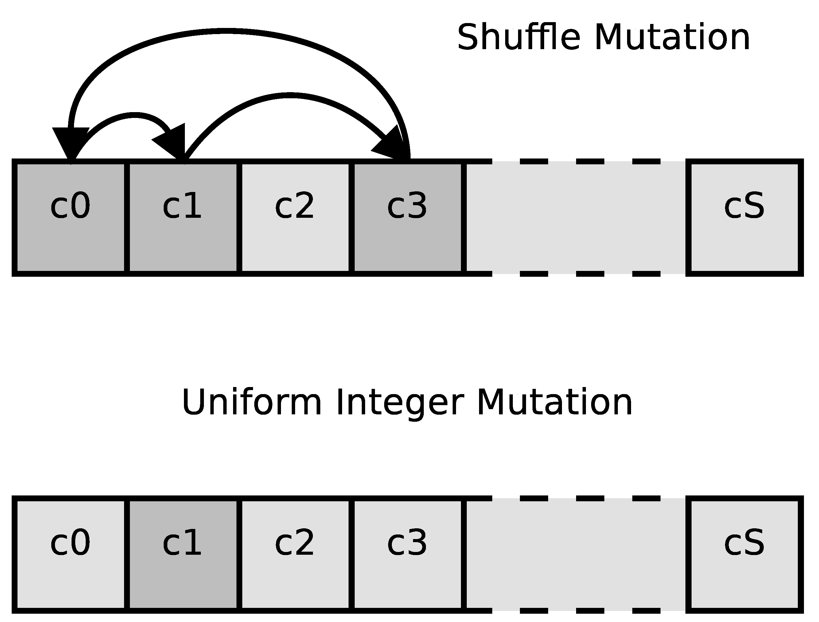
The mutation operator is called on each individual within the population with a probability that we call . Mutation alters one or more genes of the selected chromosome. Multiple mutation operators can be implemented. In our study, we consider two types of mutation operators:
- Shuffle mutation is a mutation where the mutated individual takes the genes of original chromosome applying a permutation to them. An example of shuffle mutation is shown in the upper part of Figure 2, where the genes that are involved in the mutation are marked with a darker color and arrows are used to show the genes permutation.
- Uniform Integer mutation is a mutation operator in which one or more genes are modified. The value of the affected genes is replaced using a uniform random distribution. In Figure 2, this mutation operator is shown in the lower part of the image, and the affected gene is marked with a darker color.
3.4. Crossover Operator
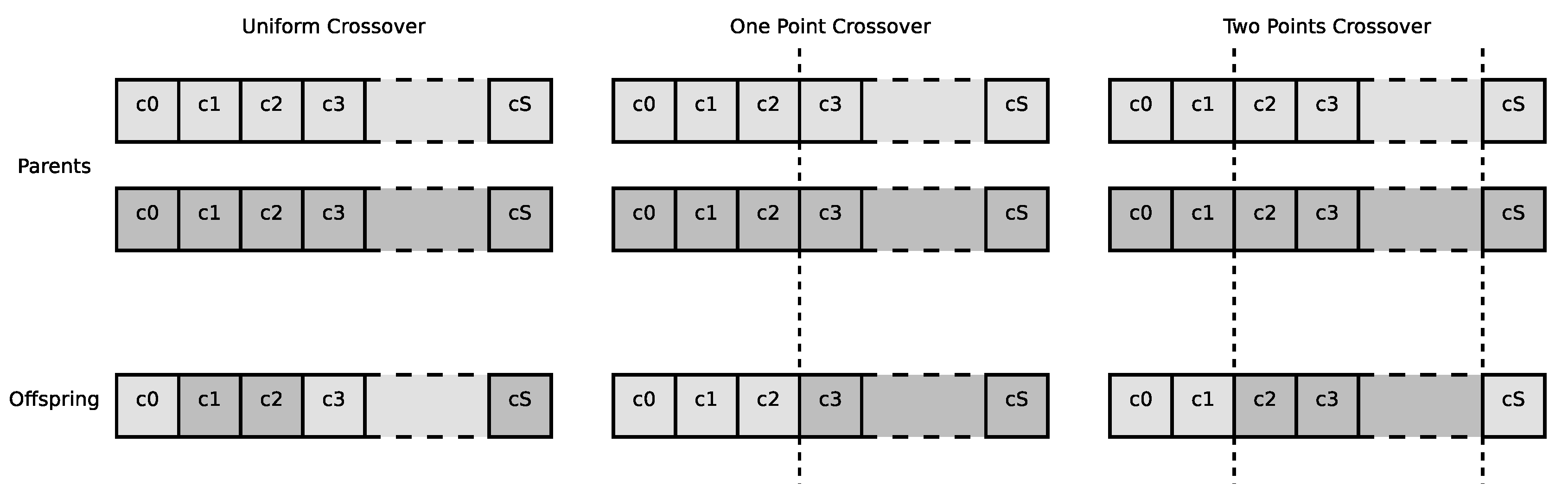
The crossover operation takes two individuals and then mates them to create two new individuals (offspring) that inherit their genes form the two parents. In the sensitivity analyses in Section 4, we will refer to the probability of selecting an individual for a crossover operation as . There are several possible crossover operators. In our analysis, we consider the following options.
- Uniform crossover is the crossover operator where the offspring will inherit each gene from a randomly selected parent. In Figure 3, the Uniform crossover operation is shown in the leftmost of the image. Each of the parents is characterized with a color. The offspring inherits each gene from one of the parents, and the parents from which the gene is inherited is marked with the same color of the parent.
- One-Point Crossover is characterized by a splitting point in the chromosome is randomly selected. The two resulting sections of the chromosome (from beginning to the spitting point and from the splitting point to the end) are then inherited from the parents as shown in the center part of Figure 3.
- Two-Point Crossover is similar to the One Point version, but we have two splitting points, as shown in the rightmost part of Figure 3.
- Uniform Partially Matched crossover (UPMX) is a variant of the Uniform crossover operator proposed in the work by the authors of [20] that considers the possible presence of identical genetic material between the parents.
3.5. GA-Based Problem Model
We now discuss how the a GA-based model of the problem can be derived from the optimization model described in Section 2.
The fist critical choice is how to encode a solution in a chromosome. To this aim, we describe a chromosome as a sequence of S genes, with being number of sensors. The generic gene, , is represented as a an integer number from 1 to F (with being the number of fog nodes in our infrastructure) and captures the information on which fog node will receive the output of that sensor. The chromosomes contain the information of the decision variable in the problem defined in the work by the authors of Section 2. Specifically, we can define the generic gene as . As only one fog node will receive data from sensor i, due to constraint (3) in the optimization model, we can map each possible solution of the optimization problem in Section 2 into a chromosome, with no conflicts or ambiguities.
The second critical problem is the definition of the fitness function for the evaluation of the chromosomes. This design choice is straightforward because, due to the mapping between chromosomes and optimization problem solutions, we can simply adapt the objective function (1) to the GA-based model and use this function for the evaluation of individuals.
Finally, we must take into account the constraints of the optimization problem. Constraints (3) and (5) are automatically satisfied by our encoding of the chromosomes. We need to implement also constraint (4) concerning the fog node overload. We chose not to embed directly the notion of unacceptable solution in a genetic algorithm, as it may hinder the ability of the heuristic to converge towards a solution. Instead, we added this constraint into the fitness function, so that an individual that contains a solution with one or more overloaded fog nodes is characterized by a high penalty and is, therefore, likely to exit the genetic pool in few generations. To define the value of the penalty, we refer to the model used in the problem definition. In particular, for most solvers the constraint (4) must be reformulated using a lesser-or-equal relationship, rather than a lesser-to relationship. Therefore, constraint (4) becomes , with . We also leverage this alternative formulation for the GA-based model, forcing the penalty in such a way that if there is overload, the processing time contribution to the objective function becomes equal to .
4. Experimental Results
We now present the main findings of our research. We start by introducing the reference scenario of our experiments. Next, we compare the ability to achieve an optimal solution of the GA-based approach with the AMPL-based [21] model solved using KNITRO [15]. In the remainder of the paper, we discuss the sensibility of the GA-based heuristic with respect its main parameters: the number of generations, the evolutionary strategies and operators, the probability of mutation and crossover, and the population size.
4.1. Experimental Testbed
To evaluate the viability of our proposal, we consider a fog scenario characterized by (1) a significant number of sensors; (2) a set of fog nodes, with limited computational power that aggregate and filter the data from the sensors; and (3) a cloud data center that collects the information processed by the fog nodes. Our testbed scenario is based on a smart city whose topology is based on a real Italian city (Modena) with a population in the order of 180,000 inhabitants.
Our reference use case is a traffic monitoring application. The sensors, fog nodes, and cloud data center are shown in Figure 4 to represent the smart city scenario. To gather data concerning traffic-related measures, such as the number of cars passing in each street (with their speed), we place wireless sensors on the main streets of the city. To model the application, we referred to the Trafair Project [9], currently involving the city of Modena considered for the topology model.
The sensor map in Figure 4 is created starting from the georeferenced list of the streets of the cities characterized by higher volumes of traffic: we assume to have one sensor for each one of these streets. Furthermore, we selected a group of six buildings that host offices of the municipality and are interconnected with a high speed metropolitan area network: each one of these buildings is assumed to host a fog node. The final scenario is composed of a 89 sensors and six fog nodes. The interconnection between fog nodes and sensors is characterized by a delay that we model using the euclidean distance between the nodes. The average delay is in the order of 10 ms, which is consistent with a geographic network. Finally, we assume to have only one cloud data center, which is located where the Modena municipality data center actually is, and is connected to the fog nodes through low latency links not considered in the optimization model.
Concerning the traffic model, we describe each scenario based on two metrics. The first metric is the average load of the system, , and the other parameter, , represents the ratio between the average network delay () and the average service time (). Specifically, we define the two parameters as
In our experiments, we consider several scenarios, corresponding to different combinations of these parameters, to analyze the performance of the GA-based solution for the sensor mapping problem. For example, a scenario where and (corresponding to the bottom right corner of Figure 5) represents a case where the network delay is much lower than the average job service time, and the processing demand on the system is high. This means that the scenario is CPU-bound because managing the computational requests is likely to be the main driver to optimize the objective function. On the other hand, a scenario where and (top left corner of Figure 5) is a scenario characterized by a low workload intensity and a network delay comparable with service time of a job, where it becomes important to optimize also the network contribution to the objective function. Throughout our experiments, we first consider the implementation of the model discussed in Section 2, using the AMPL language [21] and KNITRO [15] as the solver. Due to the nature of the problem, we were not able to let the solver run until the convergence. Instead, we placed a walltime limit of 120 minutes, with a 16-core CPU and 16 concurrent threads. We compare the results of this solver with the GA-based implementation, that uses the Distributed Evolutionary Algorithms in Python (DEAP) framework [19]. Using the same framework, we also evaluate and compare several evolutionary strategies and operators, as described in Section 3.
When evaluating the GA-based approach, we ran the experiments 100 times and reported the main performance metrics in the form of average value and confidence interval. In particular, for the confidence interval, we consider a span of , where is the standard deviation that accounts for ≈95% of the samples. The genetic algorithm considers the default parameters shown in Table 2, which were selected after some preliminary experiments. Furthermore, when considering the convergence speed, we consider as the convergence criteria the case of a fitness value within 1% of the optimum value obtained using the AMPL solver.
4.2. Comparison of Solver and GA-Based Approaches
The first analysis of our research compares the difference between the solution found by the genetic algorithm and the one obtained by the KNITRO solver. To this aim, we introduce as the main performance metric the discrepancy defined as follows,
where is the value of the objective function for the best solution found by the solver and is the value based on the best solution found using the genetic algorithm. Note that the run with KNITRO is not guaranteed to reach optimality because we stop the solver after a given amount of time. Therefore, in some cases, the genetic algorithm may outperform the solver, resulting in , as we will see in the results.
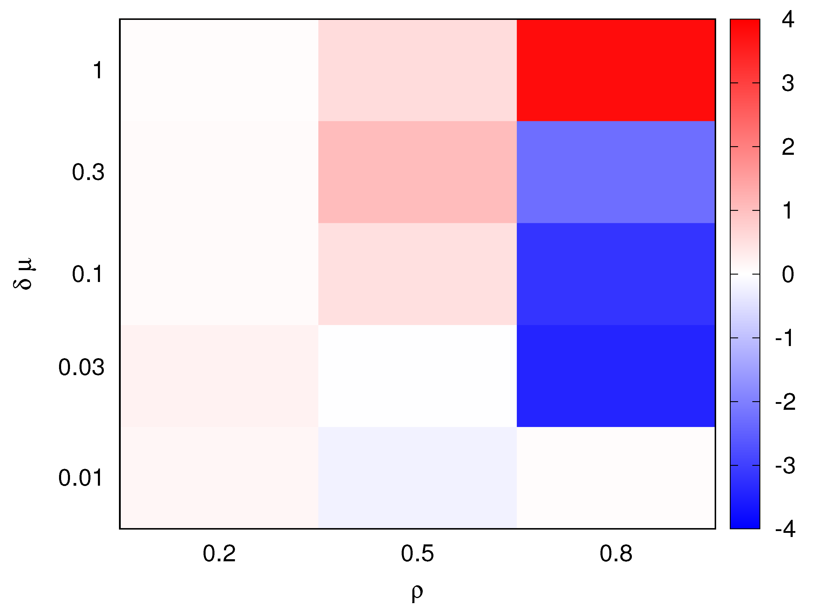
Figure 5 shows as an heatmap the value of for ranging from 0.2 to 0.8 and ranging from 0.01 to 1. In the color-coded representation of , blue hues refer to a better performance of the genetic algorithm, while red hues correspond to better performance of the solver. From this comparison, we observe that the performance of the two approaches are similar; the genetic algorithm provides slightly better performance in some cases (e.g., for , we have ) and the solver prevailing in other cases (for , we have ). Note that most differences occur for , that is, when the risk of overloading the fog nodes is higher and the value of the objective function is highly variant with respect to the considered solution.
Using this heatmap, we select two relevant cases that will be used throughout the remaining of the paper, to analyze the stability of the genetic algorithm behavior: we consider an intermediate value for the load (); whereas, for the delay impact, we consider three scenarios in the range of to to fully explore the variations in problem properties from the solver point of view.
4.3. Convergence Analysis of GAs
The second critical analysis concerns the impact of the number of generations on the performance of the genetic algorithm. We carry out this analysis for the two previously presented two scenarios, that is, , and , .
In this, and the subsequent, evaluation, we consider the previously introduced discrepancy between the GAs and the solver (). The value of is measured at every generation for the GA (compared with the final output of the solver). This allows us to evaluate if the population is converging over the generations to an optimum.
Figure 6 presents the results of this analysis. Specifically, we consider the evolution of for the considered scenarios through 300 generations of the genetic algorithm. The graph shows also an horizontal line at the value of 1%: we consider that the genetic algorithm has reached convergence when , and we consider the generation when this condition is verified as a metric to measure of how fast the algorithm can find a suitable solution. Note that, given the generally low value of , this convergence criteria returns values quite similar to the more common formulation where convergence is defined on the basis of being close (i.e., within 1%) to the best result achieved with the genetic algorithm itself.
Comparing the three curves, we observe two highly different behaviors. On one hand, for the curve characterized by (curve marked with filled triangles in Figure 6), we observe a clear descending trend. At the opposite end of the behavior spectrum, the curve for (curve marked with filled squares), is characterized by a value of that is very low right from the first generation and remains stable over the generations. The third curve (, marked with filled circles) is similar to the case with , even if a small descending trend can be observed in the first generations. The reason for this behavior can be explained considering the nature of the problem, where the objective function depends on two main contributions: the processing time (that depends mainly on the ability of the algorithm to distribute fairly the sensors among the fog nodes) and the network latency, that depends on the ability of the algorithm to map the sensors on the closest fog node. When and , the impact of the second contribution is reduced by one or two orders of magnitude compared to the case . Therefore, any solution that provides a good level of load sharing will be close to the optimum. As the genetic algorithm initializes the chromosomes with a random solution (with a uniform probability distribution), it may have one or more individuals from the first generation that provide very good performance. Further evolution of the population provides limited benefit (due to the reduced weight of the network latency component) in explaining the stable values of over the generations. The case when is remarkably different as the two contributions to the objective function have a comparable impact. Therefore, the genetic algorithm must evolve through the generations to explore a large space of solutions to find good individuals letting the population evolve.
4.4. Comparison of Evolutionary Strategies and Operators
We now discuss how the considered evolutionary strategies and operators affect the performance of the genetic algorithm. In these analyses, we will consider two main metrics: the best value of over the generations introduced in Section 4.2 (we recall that we run the algorithm for 300 generations), and the number of generations required to reach convergence, introduced in Section 4.3. For each of the two metrics, we record the average value over the 100 repetitions of the experiments and a confidence interval that accounts for ~95% of the results.
Table 3 shows the value of the considered metrics as a function of different evolutionary strategies, selection operators, mutation operators, and crossover operators. Each of these options has been introduced and described in Section 3.
A first result from the values in the table is the confirmation of the main difference between the considered scenarios. When and , the convergence occurs after just a few generations (typically right in the initial population) because the balancing part of the solution is reached easily; whereas, the network part, which receives the most benefit from population evolution, plays a minor role in the objective function. As a consequence, the impact of most considered options (that drive the evolution of the population) is reduced. On the other hand, the scenario with provides a more significant comparison of the alternatives. Also note that the best solution may depend on the scenario, as the inner nature of the problem may change as the balance in the contributions to the objective function shifts.
Starting from the evolutionary strategies, we observe that both the simple strategy and the alternative provide similar results, both in terms of objective function value and in terms of convergence. However, due to the additional complexity of the strategy (that adds additional parameters to the algorithm). we consider the more straightforward simple strategy as the best option.
Switching to the selection operators, we observe a major difference in the performance of the two alternatives (roulette and tournament selection). In the considered problem, the roulette selection tends to keep over the generations also unfit individuals, rather than purging them from the genetic pool. This hinders the convergence, as shown by the results of our experiments where the roulette selection is outperformed by the alternative in every considered scenario both in terms of and in terms of number of generations for convergence. Indeed, the roulette selection provides a good behavior when there is a difference that spans order of magnitude in the objective function, which is unlikely to occur in this type of problem. The tournament operator, instead, provides a good ability in filtering individuals from a generation to the next, guaranteeing lower values of (we recall that the best value of is computed over the span of 300 generations; so, even if convergence occurs in the initial population, we may experience a positive impact of the strategy on the final value of ).
If we consider mutation operators, we observe another effect of the changes in the problem nature with the different scenarios. For and , the Shuffle operator is better, because it preserves the most important characteristics that is the load balancing. However, this behavior has a negative impact in the scenario as it hinders a more free exploration of the solution space. On the other hand, a uniform mutation operator provides better performance for the scenario, but at the expense of a less effective search for the optimum when or .
Finally, we compare the four crossover operators. The basic performance of these operators are quire similar, with a limited difference in both and in the number of generations to reach convergence. We also observe the opposite behavior between the scenarios where the load balancing is more important than the search for the closest fog nodes ( and ) compared to the opposite case, where distance reduction through optimized topology plays an important role in performance (). However, due to the reduced impact of this parameter, we consider as the best option the uniform crossover, due to its fast and simple implementation and due to its stable performance over the different scenarios.
4.5. Sensitivity to Population Size
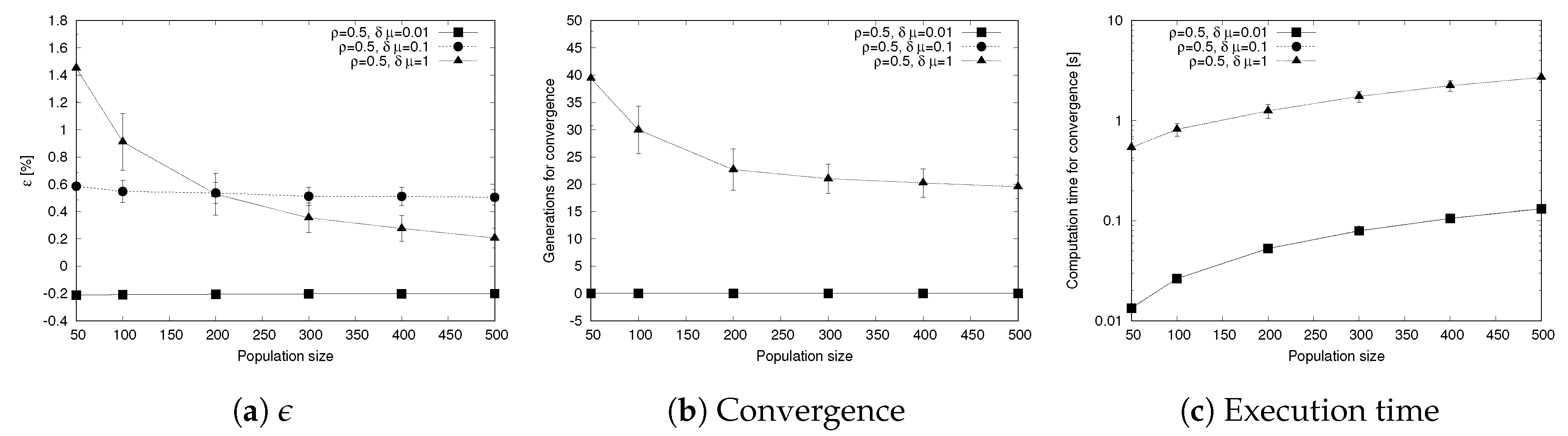
As an additional analysis we evaluate how the population size affects the performance of the genetic algorithm. To this aim, we change the population size from 50 to 500 individuals and we measure the difference in the objective function , the generations required to reach convergence and the execution time considered as the time elapsed until the algorithm reaches the convergence criteria (the main results are shown in Figure 7). Each metric also shows the confidence intervals, represented with error bars in the graphs of Figure 7.
The first significant result, shown in Figure 7a, comes from the evolution of with the population size: in this case, we show that for the more challenging scenario , increasing the population has a positive impact as it helps reducing the best value of reached. On the other hand, the other scenarios, and , show that the impact of the population size is less evident, as the exploration of the solution space improving the existing solutions has a limited effect. In a similar way, the behavior of the other main metric, that is the number of generations to reach convergence, remains stable for the scenarios and , while drops with the population when , due to the more efficient exploration of the solution space when the population is higher.
Another interesting result, shown in Figure 7c, concerns the time to execute the genetic algorithm until convergence is reached (as the result of this experiment provides values spanning over multiple orders of magnitude, we use a logarithmic scale for the y axis). We observe that for and , the time to reach convergence grows linearly (the logarithmic scale results in a curve that is not a straight line) and corresponds with the setup time of the algorithm, as convergence is reached in the first generation, as shown in Figure 7b. For the case where , the number of generations to convergence decreases with the population size. However, this effect is not enough to compensate the higher computation time needed to handle a larger population, resulting in a curve that is monotonically increasing with the population size, even if the growing rate is less evident in the first part of the graph (i.e., for populations of 200 individuals or less) compared with the other curves.
4.6. Sensitivity to Mutation and Crossover Probability
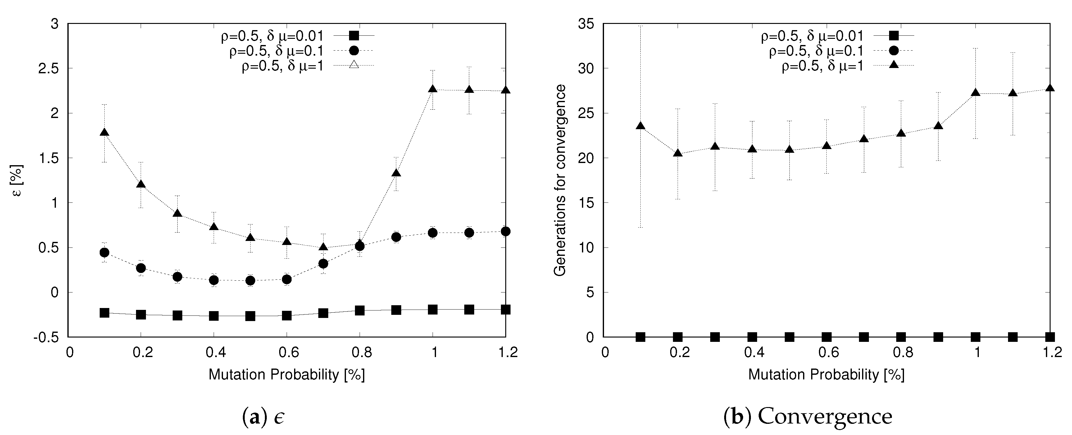
As a final analysis, we consider the sensitivity of the genetic algorithm to the two probabilities that define the evolution of the population, that is, the mutation probability and the crossover probability .
Concerning the mutation probability, Figure 8 shows how this parameter affects the ability of the algorithm to reach a value close to the solver-based output through the metric (Figure 8a) and how many generations it takes to converge (Figure 8b). We recall that, as the scenarios and achieve a value of in the first generation, the number of generations to reach convergence is not meaningful in these cases. Focusing on the metric, we observe for the scenarios a U-shaped curve that is more evident as increases. In this curve both low values () and high values () result in poor performance while values in the range result in low values of .
This behavior is explained considering the two-fold impact of mutations. On one hand, a low value of hinders the ability to explore the solutions space by creating variations in the genetic material. On the other hand, an higher mutation rate may simply reduce the ability of the algorithm to converge, because the population keeps changing too rapidly and good genes cannot be passed through the generations. The low values of has an interesting effect on the convergence curve for in Figure 8b: low mutation rates result in a poor ability to explore the solution space, with a high variance in the number of generations to reach convergence; this value depends significantly on the initial population setup.
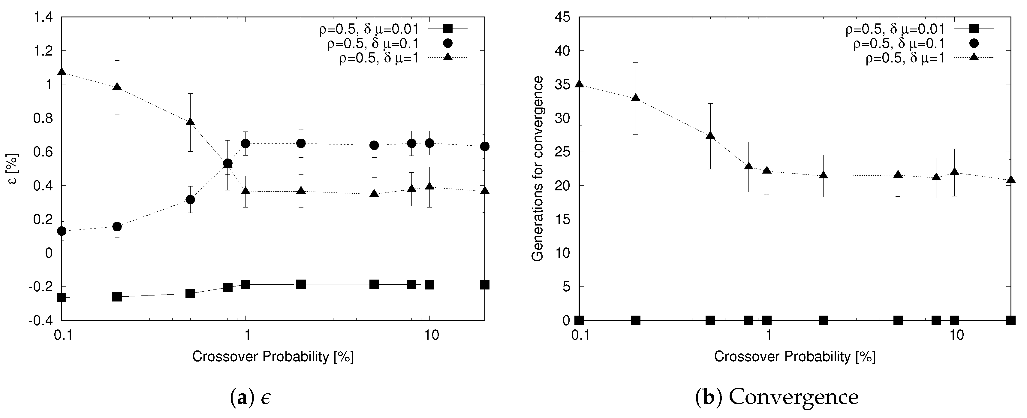
The analysis shown in Figure 9 evaluates the impact of the probability of selecting an individual for a crossover operation . Again, both (Figure 9a) and the generations reach convergence (Figure 9b) as a function of this parameter. As we change the probability over a large range of values (from 0.1% to 20%), we use a logarithmic scale for the x-axis. From the analysis, we observe that also crossover probability has a major impact on the performance of the genetic algorithm, but this parameter has a different effect on the algorithm depending on the considered scenario. For , low values of reduce the ability of the algorithm to converge rapidly; where, for higher values (that is ), this behavior does not occur. The reason for this is that a low crossover probability hinders the distribution of good genes in the population, thus slowing down the improvement of the population. For and , the effect is opposite because for the exploration of the solution space, mutation is more important than crossover and a high crossover rate interferes with the mutation operator (when crossover is applied mutation does not occur) hindering its action.
5. Related Work
The explosive growth in the generation of data and the need for their processing to provide innovative services and applications has recently led researchers to focus on fog computing solutions to complement the cloud systems capabilities. Constantly exchanging localized data from and to the remote cloud, indeed, tends to be inefficient under different points of view, thus motivating fog computing to partially process workload and data locally on fog nodes [3,5,22,23].
A survey discussing representative application scenarios and identifying various issues related to design and implementation of fog computing systems can be found in the work by the authors of [3], where the work by the authors of [23] provides an overview of the core issues, challenges, and future research directions in fog-enabled orchestration for IoT services, focusing on smart cities as main motivating example of the research. Also our study considers the smart cities as a meaningful scenario where large amount of sensors and smart devices produce a huge volume of data on a geographically distributed area. Specifically, we focus on the specific issue of distributing the incoming workload over the fog nodes to minimize communication latency while avoiding overload.
Some existing studies focus on the issue of allocating the processing tasks coming from the fog nodes to the cloud nodes to optimize performance and reduce latency. Among these studies, Deng et al. [5] explore the trade-off between power consumption and transmission delay in the fog-cloud computing system, formulating an optimization of the allocation problem among fog and cloud nodes. The study by the authors of [6] explicitly focuses on the issue of minimizing the service delay in IoT-fog-cloud application scenarios, proposing a delay-minimizing policy for fog nodes: in contrast to other proposals in literature, the proposed policy employs fog-to-fog communication to reduce the service delay by sharing load. Similarly, in the work by the authors of [24], an offloading mechanism is proposed where a fog-to-fog collaboration based on the FRAMES load balancing scheme aims to reduce the overall latency experienced by the services. Note that these studies do not consider the issue of mapping data sources on the fog nodes: the fog nodes directly communicate with the mobile users through single-hop wireless connections using the off-the-shelf wireless interfaces (e.g., WiFi, Bluetooth, LR-WPANs, etc.) or the considered scenario envisions a domain of IoT nodes (in a factory, for instance) that communicate with a domain of fog nodes, associated with the specific domain application(s). On the other hand, our study focuses on the issue of optimizing the mapping of the workload coming from data sources over the fog nodes.
Few studies assume a flexible mapping of data sources over the fog nodes. The study by the authors of [25] proposes a framework to design services for smart building-based on edge and fog computing paradigms, where the IoT sensors communicate data through the MQTT protocol: this study assumes a potential flexible mapping for design purposes but does not propose any specific (optimized) solution to address this issue. The authors of [26,27] propose a coordination scheme between cloud and fog nodes applied to a healthcare-driven IoT application and to a real-time streaming application, respectively. In these studies, the data sources can choose to connect to the fog node or directly to the cloud data center according to specific conditions. However, in our solution the sensors always send data to an intermediate fog node to be selected within the fog layer to optimize the service performance.
Among the studies focusing on fog computing applied to the same context of our paper, in the work by the authors of [22], a hierarchical 4-layer fog computing architecture is proposed for big data analysis in smart cities. The layered fog computing network exploits the natural characteristic of geodistribution in big data generated by massive sensors, performing latency-sensitive applications and providing quick control loop to ensure the safety of critical infrastructure components. In this paper, the mapping between fog nodes and sensors is fixed: each fog node is connected to and responsible for a local group of sensors that cover a neighborhood or a small community.
The authors of [28] consider Data Stream Processing (DSP) applications and, specifically, the so-called operator placement problem, that is the allocation of DSP operator on fog nodes with the goal of optimizing the applications Quality of Service (QoS). The optimal DSP placement is modeled as an Integer Linear Programming (ILP) problem. In this case the authors made the assumption that it is possible to split the incoming data flow for parallel processing, while we consider generic applications where this assumption may not be true.
Regarding the use of Genetic Algorithms (GAs), they have been successfully applied to the context of cloud computing in recent literature. The study by the authors of [7] exploits GAs to produce a suitable and scalable solution for the Software as a Service (SaaS) Placement Problem [7], whereas Karimi et al. [29] propose a QoS-aware service composition for cloud computing systems based on GAs. A previous version of the paper by the same authors was presented in [8], proposing the use of a GA-based heuristic to map data flows over the fog nodes. However, this paper represents a clear step ahead with respect to the previous work, with improvements regarding both the theoretical contribution and the experimental setup, including new scenarios and sensitivity analysis.
6. Conclusions and Future Work
This paper presents a solution based on fog computing to address the issues of the typical scenario of a smart city, where sensors or smart devices disseminated over a geographic area produce a large amount of data. We pointed out that a traditional cloud infrastructure, with all data flows converging on a single cloud data center (or, at most, on few data centers) is at risk of network congestion. Moreover, as some applications in such scenarios are latency-sensitive (e.g., applications related to automated traffic management) or produce a bulk of data that could create congestion at the network level (e.g., widespread sensors for environmental analysis), the most suitable approach is to exploit a layer of intermediate fog nodes located as close as possible to the data sources to perform preprocessing (e.g., filtering and aggregation) or latency-critical tasks.
The innovative paradigm of fog computing opens several new issues. In this paper, we focus on the problem of mapping the data streams produced by the sensors over the fog nodes. We provided a formal model for the problem of minimizing the overall latency experienced in the system, considering both data transfer and processing times. Furthermore, we proposed an heuristic algorithm, based on genetic programming to solve the problem without the need to rely on an external solver.
The proposed solution is evaluated in the context of a realistic smart city scenario. The experiments show the excellent performance of the proposed genetic algorithm to solve the mapping problem. Moreover, different evolutionary strategies and genetic operators are compared to identify the best performing one in the considered scenario. Finally, we demonstrate the stability of the proposed heuristic through a sensitivity analysis on its main parameters, such as the number of generations, the probability of mutation and crossover, and the population size.
As a future work, we plan to extend the current research, taking into account more complex scenarios that involve dynamic changes in the workload, for example, to introduce mobility in the data sources or to consider adaptive sampling techniques at the sensor level producing dynamic outgoing data rate. To support these news scenarios, we plan to provide contributions not only in terms of the definition of the topology, but also at the level of adaptive algorithms proposal.
Author Contributions
Theoretical model: R.L.; optimization problem software development: C.C.; genetic algorithm software development: R.L.; experiments: C.C. and R.L.; writing: C.C. and R.L.
Funding
This research received no external funding.
Acknowledgments
The authors acknowledge the support in the preliminary stages of the research of their students Davide Casalini and Robert Covic.
Conflicts of Interest
The authors declare no conflict of interest.
References
- Liu, J.; Li, J.; Zhang, L.; Dai, F.; Zhang, Y.; Meng, X.; Shen, J. Secure intelligent traffic light control using fog computing. Future Gener. Comput. Syst. 2018, 78, 817–824. [Google Scholar] [CrossRef]
- Sasaki, K.; Suzuki, N.; Makido, S.; Nakao, A. Vehicle Control System Coordinated Between Cloud and Mobile Edge Computing. In Proceedings of the 2016 55th Annual Conference of the Society of Instrument and Control Engineers of Japan (SICE), Tsukuba, Japan, 20–23 September 2016; pp. 1122–1127. [Google Scholar]
- Yi, S.; Li, C.; Li, Q. A Survey of Fog Computing: Concepts, Applications and Issues. In Proceedings of the 2015 Workshop on Mobile Big Data, Hangzhou, China, 21 June 2015; ACM: New York, NY, USA, 2015; pp. 37–42. [Google Scholar] [CrossRef]
- Dastjerdi, A.V.; Buyya, R. Fog Computing: Helping the Internet of Things Realize Its Potential. Computer 2016, 49, 112–116. [Google Scholar] [CrossRef]
- Deng, R.; Lu, R.; Lai, C.; Luan, T.H.; Liang, H. Optimal workload allocation in fog-cloud computing toward balanced delay and power consumption. IEEE Internet Things J. 2016, 3, 1171–1181. [Google Scholar] [CrossRef]
- Yousefpour, A.; Ishigaki, G.; Jue, J.P. Fog Computing: Towards Minimizing Delay in the Internet of Things. In Proceedings of the 2017 IEEE International Conference on Edge Computing (EDGE), Honolulu, HI, USA, 25–30 June 2017; pp. 17–24. [Google Scholar] [CrossRef]
- Yusoh, Z.I.M.; Tang, M. A Penalty-Based Genetic Algorithm for the Composite SaaS Placement Problem in the Cloud. In Proceedings of the IEEE Congress on Evolutionary Computation, Barcelona, Spain, 18–23 July 2010; pp. 1–8. [Google Scholar] [CrossRef]
- Canali, C.; Lancellotti, R. A Fog Computing Service Placement for Smart Cities based on Genetic Algorithms. In Proceedings of the International Conference on Cloud Computing and Services Science (CLOSER 2019), Crete, Greece, 2–4 May 2019. [Google Scholar]
- Bigi, A.; Veratti, G.; Fabbi, S.; Ziven, O.; Po, L.; Ghermandi, G. Forecast of the Impact by Local Emissions at An Urban Micro Scale by the Combination of Lagrangian Modelling and Low Cost Sensing Technology: The TRAFAIR Project. In Proceedings of the 19th International Conference on Harmionisation within Atmospheric Dispersion Modelling for Regulatory Purposes, Bruges, Belgium, 3–6 June 2019. [Google Scholar]
- Shojafar, M.; Canali, C.; Lancellotti, R. A Computation- and Network-Aware Energy Optimization Model for Virtual Machines Allocation. In Proceedings of the International Conference on Cloud Computing and Services Science (CLOSER 2017), Porto, Portugal, 24–26 April 2017. [Google Scholar]
- Shojafar, M.; Canali, C.; Lancellotti, R.; Abolfazli, S. An Energy-aware Scheduling Algorithm in DVFS-enabled Networked Data Centers. In Proceedings of the 6th International Conference on Cloud Computing and Services Science, Rome, Italy, 23–25 April 2016; Volumes 1–2. [Google Scholar]
- Noshy, M.; Ibrahim, A.; Ali, H. Optimization of live virtual machine migration in cloud computing: A survey and future directions. J. Netw. Comput. Appl. 2018, 110, 1–10. [Google Scholar] [CrossRef]
- Duan, H.; Chen, C.; Min, G.; Wu, Y. Energy-aware scheduling of virtual machines in heterogeneous cloud computing systems. Future Gener. Comput. Syst. 2017, 74, 142–150. [Google Scholar] [CrossRef]
- Ardagna, D.; Ciavotta, M.; Lancellotti, R.; Guerriero, M. A hierarchical receding horizon algorithm for QoS-driven control of Multi-IaaS applications. IEEE Trans. Cloud Comput. 2018. [Google Scholar] [CrossRef]
- Knitro Website. Available online: https://www.artelys.com/solvers/knitro/ (accessed on 10 July 2019).
- Canali, C.; Lancellotti, R. Scalable and automatic virtual machines placement based on behavioral similarities. Computing 2017, 99, 575–595. [Google Scholar] [CrossRef]
- Binitha, S.; Sathya, S.S. A survey of bio inspired optimization algorithms. Int. J. Soft Comput. Eng. 2012, 2, 137–151. [Google Scholar]
- Back, T.; Fogel, D.; Michalewicz, Z. Evolutionary Computation 1: Basic Algorithms and Operators; CRC Press: Boca Raton, FL, USA, 2002. [Google Scholar]
- DEAP: Distributed Evolutionary Algorithms in Pyton. 2018. Available online: https://deap.readthedocs.io (accessed on 19 September 2019).
- Cicirello, V.A.; Smith, S.F. Modeling GA Performance for Control Parameter Optimization. In Proceedings of the 2nd Annual Conference on Genetic and Evolutionary Computation, Las Vegas, NV, USA, 10–12 July 2000; Morgan Kaufmann Publishers Inc.: San Francisco, CA, USA, 2000; pp. 235–242. [Google Scholar]
- AMPL: Streamlined Modeling for Real Optimization. 2018. Available online: https://ampl.com/ (accessed on 19 September 2019).
- Tang, B.; Chen, Z.; Hefferman, G.; Wei, T.; He, H.; Yang, Q. A Hierarchical Distributed Fog Computing Architecture for Big Data Analysis in Smart Cities. In Proceedings of the ASE BigData & SocialInformatics 2015, Kaohsiung, Taiwan, 7–9 October 2015; ACM: New York, NY, USA, 2015; pp. 1–6. [Google Scholar] [CrossRef]
- Wen, Z.; Yang, R.; Garraghan, P.; Lin, T.; Xu, J.; Rovatsos, M. Fog orchestration for internet of things services. IEEE Internet Comput. 2017, 21, 16–24. [Google Scholar] [CrossRef]
- Al-khafajiy, M.; Baker, T.; Al-Libawy, H.; Maamar, Z.; Aloqaily, M.; Jararweh, Y. Improving fog computing performance via Fog-2-Fog collaboration. Future Gener. Comput. Syst. 2019, 100, 266–280. [Google Scholar] [CrossRef]
- Ferrández-Pastor, F.J.; Mora, H.; Jimeno-Morenilla, A.; Volckaert, B. Deployment of IoT edge and fog computing technologies to develop smart building services. Sustainability 2018, 10, 3832. [Google Scholar] [CrossRef]
- Maamar, Z.; Baker, T.; Faci, N.; Ugljanin, E.; Khafajiy, M.A.; Burégio, V. Towards a Seamless Coordination of Cloud and Fog: Illustration through the Internet-of-Things. In Proceedings of the 34th ACM/SIGAPP Symposium on Applied Computing, Limassol, Cyprus, 8–12 April 2019. [Google Scholar]
- Nair, B.; Saira Bhanu, S.M. Fog-Cloud Collaboration for Real-Time Streaming Applications: FCC for RTSAs. In Handbook of Research on the IoT, Cloud Computing, and Wireless Network Optimization; IGI Global: Hershey, PA, USA, 2019. [Google Scholar]
- Cardellini, V.; Grassi, V.; Lo Presti, F.; Nardelli, M. Optimal Operator Placement for Distributed Stream Processing Applications. In Proceedings of the 10th ACM International Conference on Distributed and Event-Based Systems, Irvine, CA, USA, 20–24 June 2016; ACM: New York, NY, USA, 2016; pp. 69–80. [Google Scholar] [CrossRef]
- Karimi, M.B.; Isazadeh, A.; Rahmani, A.M. QoS-aware service composition in cloud computing using data mining techniques and genetic algorithm. J. Supercomput. 2017, 73, 1387–1415. [Google Scholar] [CrossRef]
Figure 1.
Cloud and Fog infrastructures.

Figure 2.
Examples of mutation operators.

Figure 3.
Examples of crossover operators.

Figure 4.
Smart city scenario.

Figure 5.
Performance comparison: [%].

Figure 6.
Convergence analysis.

Figure 7.
Sensitivity to population size.

Figure 8.
Sensitivity to Mutation Probability .

Figure 9.
Sensitivity to crossover probability .


Table 1.
Notation.
| Symbol | Meaning/Role |
|---|---|
| Decision Variables | |
| Sending data flow from sensor i to fog node j | |
| Model Parameters | |
| Set of sensors | |
| Set of Fog nodes | |
| Outgoing data rate from sensor i | |
| Incoming data rate at fog node j | |
| Processing time at fog node j | |
| Communication latency between sensor i to fog node j | |
| Model Variables | |
| i | Index of a sensor |
| j | Index of a fog node |
Table 2.
Default genetic algorithm (GA) parameters.
| Parameter | Value |
|---|---|
| Strategy | Simple strategy |
| Selection | Tournament selection |
| Mutation | Uniform Integer mutation |
| Crossover | Uniform crossover |
| Population size | 200 |
| Generations | 300 |
| 0.8% | |
| 0.8% |
Table 3.
Evolutionary strategies.
| Strategy or | , | , | , | |||
|---|---|---|---|---|---|---|
| Operator | [%] | # Gen. | [%] | # Gen. | [%] | # Gen. |
| Evolutionary Strategies | ||||||
| Simple | ||||||
| Selection Operators | ||||||
| Tournament | ||||||
| Roulette | ||||||
| Mutation Operators | ||||||
| Shuffle | ||||||
| Uniform Int | ||||||
| Crossover Operators | ||||||
| Uniform | ||||||
| One Point | ||||||
| Two Points | ||||||
| UPMX | ||||||
© 2019 by the authors. Licensee MDPI, Basel, Switzerland. This article is an open access article distributed under the terms and conditions of the Creative Commons Attribution (CC BY) license (http://creativecommons.org/licenses/by/4.0/).
Share and Cite
MDPI and ACS Style
Canali, C.; Lancellotti, R. GASP: Genetic Algorithms for Service Placement in Fog Computing Systems. Algorithms 2019, 12, 201. https://0-doi-org.brum.beds.ac.uk/10.3390/a12100201
AMA Style
Canali C, Lancellotti R. GASP: Genetic Algorithms for Service Placement in Fog Computing Systems. Algorithms. 2019; 12(10):201. https://0-doi-org.brum.beds.ac.uk/10.3390/a12100201
Chicago/Turabian StyleCanali, Claudia, and Riccardo Lancellotti. 2019. "GASP: Genetic Algorithms for Service Placement in Fog Computing Systems" Algorithms 12, no. 10: 201. https://0-doi-org.brum.beds.ac.uk/10.3390/a12100201
Note that from the first issue of 2016, this journal uses article numbers instead of page numbers. See further details here.