(Hyper)Graph Embedding and Classification via Simplicial Complexes


1
Department of Information Engineering, Electronics and Telecommunications, University of Rome “La Sapienza”, Via Eudossiana 18, 00184 Rome, Italy
2
Department of Environment and Health, Istituto Superiore di Sanità, Viale Regina Elena 299, 00161 Rome, Italy
*
Author to whom correspondence should be addressed.
Algorithms 2019, 12(11), 223; https://0-doi-org.brum.beds.ac.uk/10.3390/a12110223
Submission received: 26 September 2019
/
Revised: 21 October 2019
/
Accepted: 24 October 2019
/
Published: 25 October 2019
(This article belongs to the Special Issue Granular Computing: From Foundations to Applications)
Abstract
:This paper investigates a novel graph embedding procedure based on simplicial complexes. Inherited from algebraic topology, simplicial complexes are collections of increasing-order simplices (e.g., points, lines, triangles, tetrahedrons) which can be interpreted as possibly meaningful substructures (i.e., information granules) on the top of which an embedding space can be built by means of symbolic histograms. In the embedding space, any Euclidean pattern recognition system can be used, possibly equipped with feature selection capabilities in order to select the most informative symbols. The selected symbols can be analysed by field-experts in order to extract further knowledge about the process to be modelled by the learning system, hence the proposed modelling strategy can be considered as a grey-box. The proposed embedding has been tested on thirty benchmark datasets for graph classification and, further, we propose two real-world applications, namely predicting proteins’ enzymatic function and solubility propensity starting from their 3D structure in order to give an example of the knowledge discovery phase which can be carried out starting from the proposed embedding strategy.
1. Introduction
Graphs are powerful data structures that can capture topological and semantic information from data. This is one of the main reasons they are commonly used for modelling several real-world systems in fields such as biology and chemistry [1,2,3,4,5,6,7,8], social networks [9], telecommunication networks [10,11] and natural language processing [12,13,14].
However, solving pattern recognition problems in structured domains such as graphs pose additional challenges. Indeed, many structured domains are also non-metric in nature [15,16,17] and patterns lack any geometrical interpretation. In brief, an input space is said to be non-metric if pairwise dissimilarities between patterns lying in such space do not satisfy the properties of a metric (non-negativity, identity, symmetry and triangle inequality) [17,18].
In the literature, several strategies can be found in order to perform pattern recognition tasks in structured domains [17], namely:
- feature generation and feature engineering, where numerical features are ad-hoc extracted from the input patterns
- embedding via information granulation.
As the latter is concerned, embedding techniques are gaining more and more attention especially since the breakthrough of Granular Computing [33,34]. In short, Granular Computing is a human-inspired information processing paradigm which aims at the extraction of meaningful entities (information granules) arising from both the problem at hand and the data representation. The challenge with Granular Computing-based pattern recognition systems is that there are different levels of granularity according to which a given system can be observed [35,36,37]; nonetheless, one shall choose a suitable level of granularity for the problem at hand. These information granules are usually extracted in a data-driven manner and describe data aggregates, namely data which are similar according to structural and/or functional similarity [15,16,17]. Data clustering, for example, is a promising tool for extracting information granules [38], especially when clustering algorithms can be equipped with ad-hoc dissimilarity measures in order to deal with structured data [17,39,40,41,42]. Indeed, several works focused on extracting information granules via motifs clustering (see e.g., Refs. [43,44,45,46,47]), where a proper granulation module is in charge of extracting and clustering sub-structures (i.e., sub-graphs). The resulting clusters can be considered as information granules and the clusters’ representatives form an alphabet on the top of which the embedding procedure is performed thanks to the symbolic histograms approach [46]: let M be the size of the alphabet, each input pattern is transformed into an M-length integer-valued feature vector whose ith element contains the number of occurrences of the ith alphabet member within the pattern itself. Thanks to the embedding, the problem is moved towards a metric (Euclidean) space and plain pattern recognition algorithms can be used without alterations.
The symbols extraction and alphabet synthesis is crucial in granulation-based classifiers: the resulting embedding space must preserve (the vast majority of) the original input space properties (e.g., the more different two objects drawn from the input space are, the more distant they must appear in the embedding space.) [17,18]. Also, for the sake of modelling complexity, the size of the alphabet must be as small as possible or, specifically, the set of resulting alphabet symbols should be small, yet informative. This aspect is crucial since Granular Computing-based pattern recognition systems aim to be human interpretable: the resulting set of symbols forming the alphabet, hence pivotal for the embedding space, should allow field experts to gather further insights for the problem at hand [17].
The aim of this paper is to investigate a novel procedure for extracting meaningful information granules thanks to simplicial complexes. Conversely to network motifs and graphlets, simplicial complexes are able to capture the multi-scale/higher-order organisation in complex networks [48,49], overcoming the main limitation offered by ‘plain graphs’; that is, they only considers pairwise relations, whereas simplicial complexes (and hypergraphs, in general) also consider multi-way relations. On the top of simplicial complexes, an embedding space is built for pattern recognition purposes.
In order to show the effectiveness of the proposed embedding procedure, a set of thirty open-access datasets for graph classification has been considered. Furthermore, the proposed technique has been benchmarked against two suitable competitors and a null-model for statistical assessment. In order to stress the knowledge discovery phase offered by Granular Computing-based classifiers, additional experiments are proposed. Specifically, starting from real-world proteomic data, two problems will be addressed regarding the possibility to predict the enzymatic function and the solution/folding propensity starting from proteins’ folded 3D-structure.
This paper is organised as follows: in Section 2 the approach at the basis of work is presented by giving a brief overview of simplicial complexes (Section 2.1) before diving into the proper embedding procedure (Section 2.2); in Section 3 the results over benchmark datasets (Section 3.1) and real-world problems (Section 3.2) are shown. Section 4 remarks the interpretability of the proposed model and, finally, Section 5 concludes the paper, remarking future directions.
2. Information Granulation and Classification Systems
2.1. An Introduction to Simplicial Complexes
Let be a set of points in a multi-dimensional space equipped with a notion of distance and let be the topological space enclosing . The topological space can be described by means of its simplices, that are multidimensional objects of different order (dimension) drawn from . Formally, a k-simplex (simplex of order k) is a set of points drawn from , for example, 0-dimensional simplices correspond to points, 1-dimensional simplices correspond to lines, 2-dimensional simplices correspond to triangles, 3-dimensional simplices correspond to tetrahedrons and so on for higher-dimensional simplices. Every non-empty subset of the vertices of a k-simplex is a face of the simplex: a face is itself a simplex. Simplicial complexes [50,51] are properly constructed finite collections of simplices that are closed with respect to inclusions of the faces: if a given simplex s belongs to a given simplicial complex , then all faces of s also belong to . The order (dimension) of the simplicial complex is the maximum order of any of its simplices.
A graph , where is the set of edges and is the set of vertices, is also commonly-known as “1-skeleton” or “simplicial complex of order 1” since the only entities involved are 0-simplices (nodes) and 1-simplices (edges). However, the modelling capabilities offered by graphs are often not sufficient as they only regard pairwise relations. Indeed, for some problems (ranging from bioinformatics [52,53,54] to signal processing [55,56,57]), multi-way relations are more suited, where two or more nodes are more conveniently connected by an hyperedge (in this scenario, we are de facto talking about hypergraphs [58]). Simplicial complexes are an example of hypergraphs and therefore able to capture the multi-scale organisation in real-world complex networks [48,49].
A straightforward example in order to focus hypergraphs and complexes may regard a scientific collaboration network in which nodes are authors and edges exist whether two authors co-authored a paper. This representation does not consider the case in which three or more authors wrote a paper together or, better, it would be ambiguous: three authors (for example) can be connected by edges in a graph but this scenario is ambiguous about whether the three authors co-authored a paper or each pair of authors co-authored a paper. By using hypergraphs, the same problem can be modelled where nodes are authors and hyperedges connect groups of authors that co-authored a paper together. A more biologically-oriented example include protein interaction networks, where nodes correspond to proteins and edges exist whether they interact. Yet, this representation does not consider protein complexes [52].
In literature, several simplicial complexes have been proposed, with the Čech complex, the Alpha complex and the Vietoris-Rips complex being the most studied [50,51,59,60,61]. In order to introduce the three simplicial complexes, let be a point cloud and let be a real-valued number:
- Čech complex:
- for each subset of points, form an -ball (A ball with radius ) centred at each point in S, and include S as a simplex if there is a common point contained in all of the balls created so far.
- Alpha complex:
- for each point , evaluate its Voronoi region (i.e., the set of points closest to it). The set of Voronoi regions forms the widely-known Voronoi diagram and the nerve of the latter is usually referred to as Delaunay complex. By considering an -ball around each point , it is possible to intersect said ball with , leading to a restricted Voronoi region and the nerve of the set of restricted Voronoi regions for all points in is the Alpha complex.
- Vietoris-Rips complex:
- for each subset of points, check whether all of their pairwise distances are below . If so, S is a valid simplex to be included in the Vietoris-Rips complex.
Čech complex, Alpha complex and Vietoris-Rips complex strictly depend on , which somehow determines the ’resolution’ of the simplicial complex. Amongst the three, the Vietoris-Rips is the most used due to lower computational complexity and intuitiveness [59]. Indeed, the latter can be easily evaluated as follows [62]:
- build the Vietoris-Rips neighbourhood graph where is the set of vertices and is the set of edges, hence and if for any two nodes with
- evaluate all maximal cliques in .
The second step is due to the fact that the Vietoris-Rips complex is dually definable as the Clique complex of the Vietoris-Rips neighbourhood graph. The latter complex [48,63,64] is defined as follows:
- Clique complex:
- for a given underlying graph , the Clique complex is the simplicial complex formed by the set of vertices of its (maximal) cliques. In other words, a clique of k vertices is represented by a simplex of order .
Despite its ’minimalistic’ definition, proving that the Clique complex is a valid simplicial complex is straightforward: any subset of a clique is also a clique, meeting the requirement of being closed with respect to inclusions of the faces. A useful facet of the Clique complex relies on its parameter-free peculiarity: if the underlying 1-skeleton is available beforehand, one can directly use the Clique complex which not only does not need any scale parameter (e.g., for the Vietoris-Rips complex and the Alpha complex) but also encodes the same information as the underlying graph and additionally completes a topological object with its fullest possible simplicial structure, being it a canonical polyadic extension of existing networks (1-skeletons) [65]. Further, it is noteworthy that from the set of cliques it is possible to recover the k-faces of the simplices by extracting all -combinations of these cliques. This is crucial when one wants to study the homology of the simplicial complex which is, however, out of the scope of this paper [66,67]. Despite enumerating the maximal cliques being well-known as an NP-complete problem, several heuristics can be found in the literature [68,69,70].
2.2. Proposed Approach
2.2.1. Embedding
Let be a dataset of graphs, where each graph has the form , where is the set of vertices labels. For the sake of argument, let us consider a supervised problem, thus let be the corresponding ground-truth class labels for each of the graphs in . Further, consider to be split into three non-overlapping training, validation and test sets (, , , respectively) and, by extension, the labels are split accordingly (, , ). Let q be the number of classes for the classification problem at hand.
The first step is to evaluate the simplicial complex separately for all graphs in the three datasets splits, hence
where is a function that evaluates the simplicial complex starting from the 1-skeleton .
However, the embedding is performed on the concatenation of and or, specifically, and . In other words, the alphabet sees the concatenation of the simplices belonging to the simplicial complexes evaluated starting from all graphs in and .
In cases of large networks and/or large datasets, this might lead to a huge number of simplices which are hard to match. For example, let us consider any given node belonging to a given graph to be identified by a progressive unique number. In this case, it is impossible to match two simplices belonging to possibly two different simplicial complexes (i.e., determine whether they are equal or not). In order to overcome this problem, node labels play an important role. Indeed, a simplex can dually be described by the set of node labels belonging to its vertices. This conversion from ’simplices-of-nodes’ to ’simplices-of-node-labels’ has a three-fold meaning, especially if node labels belong to a categorical and finite set:
- the match between two simplices (possibly belonging to different simplicial complexes) can be done in an exact manner: two simplices are equal if they have the same order and they share the same set of node labels
- simplicial complexes become multi-sets: two simplices (also within the same simplicial complex) can have the same order and can share the same set of node labels
- the enumeration of different (unique) simplices is straightforward.
In light of these observations, it is possible to define the three counterparts of Equations (1)–(3) where each given node u belonging to a given simplex is represented by its node label:
Let be the set of unique (distinct) simplices belonging to the simplicial complexes evaluated from graphs in :
and let . The next step is to properly build the embedding vectors thanks to the symbolic histograms paradigm. Accordingly, each simplicial complex (evaluated on the top of a given graph, that is, 1-skeleton) is mapped into an M-length integer-valued vector as follows
where is a function that counts the number of times a appears in b.
The three sets , and are separately cast into three proper instance matrices , and . For each set, the corresponding instance matrix scores in position the number of occurrences of the jth symbol (simplex) from within the ith simplicial complex (in turn, evaluated on the top of the ith graph).
2.2.2. Classification
In the embedding space, namely the vector space spanned by the symbolic histograms of the form as in Equation (8), any classification system can be used. However, it is worth stressing the importance of feature selection whilst performing classification as per the following two (not mutually exclusive) rationales:
- there is no guarantee that all symbols in are indeed useful for the classification problem at hand
- as introduced in Section 1, it is preferable to have a small, yet informative, alphabet in order to eventually ease an a-posteriori knowledge discovery phase (less symbols to be analysed by field-experts).
For a given classification system C, let us consider its set of hyper-parameters to be tuned. Further, let be an M-length binary vector in charge of selecting features (columns) from the instance matrices (i.e., symbols from ) corresponding to non-zero elements. The tuple
can be optimised, for example, by means of a genetic algorithm [71] or other metaheuristics.
In this work, two different classification systems are investigated. The former relies on non-linear -Support Vector Machines (-SVMs) [72], whereas the latter relies on 1-norm Support Vector Machines (-SVMs) [73].
The rationale behind using the latter is as follows. -SVMs, by minimising the 1-norm instead of the 2-norm of the separating hyperplane as in standard SVMs [72,74,75], return a solution (hyperplane coefficient vector) which is sparse: this allows to perform feature selection during training.
For the sake of sketching a general framework, let us start our discussion from -SVMs which do not natively return a sparse solution (i.e., do not natively perform any feature selection). The -SVM is equipped with the radial basis function kernel:
where are two given patterns from the dataset at hand, is a suitable (dis)similarity measure and is the kernel shape parameter. The adopted dissimilarity measure is the weighted Euclidean distance:
where M is the number of features and is the binary weight for the ith feature. Hence, it is possible to define and the overall genetic code for -SVM has the form
Each individual from the evolving population exploits to train a -SVM using the parameters written in its genetic code as follows:
- trains the -SVM with regularisation parameter
The optimal hyperparameters set is the one that minimises the following objective function on :
where J is the (normalised (Originally, the informedness is defined as and therefore is bounded in . However, since the rightmost term in Equation (13) is bounded in and , we adopt a normalised version in order to ensure a fair combination.)) informedness (The informedness, by definition, takes into account binary problems. In case of multiclass problems, one can evaluate the informedness for each class by marking it as positive and then consider the average value amongst the problem-related classes.) [76,77], defined as:
whereas the rightmost term takes into account the sparsity of the feature selection vector . Finally, is a user-defined parameter which weights the contribution of performances (leftmost term) and number of selected alphabet symbols (rightmost term). As the evolution ends, the best individual is evaluated on .
As previously introduced, -SVMs minimise the 1-norm of the separating hyperplane and natively return a sparse hyperplane coefficient vector, say . In this case, the genetic code will not consider and only can be optimised. For -SVMs the genetic code has the form
where C is the regularisation parameter and are additional weights in order to adjust C in a class-wise fashion ( is not mandatory for -SVMs to work, but it might be of help in case of heavily-unbalanced classes.). Specifically, for the ith class, the misclassification penalty is given by . The evolutionary optimisation does not significantly change with respect to the -SVM case: each individual trains a -SVM using the hyperparameters written in its genetic code on and its results are validated on . The fitness function is still given by Equation (13) with in lieu of . As the evolution ends, the best individual is evaluated on .
3. Results
3.1. On Benchmark Data
In order to show the effectiveness of the proposed embedding procedure, both of the classification strategies (-SVM and -SVM) have been considered. The genetic algorithm has been configured as follows: 100 individuals per 100 generations with a strict early-stop criterion if the average fitness function over rd of the total number of generations is less than or equal to , the elitism is set to 10% of the population, the selection follows the roulette wheel heuristic, the crossover operator generates new offsprings in a scattered fashion and the mutation acts in a flip-the-bit fashion for boolean genes and adds to real-valued genes a random number extracted from a zero-mean Gaussian distribution whose variance shrinks as generations go by. The upper and lower bounds for SVMs hyperparameters are by definition, , and has entries in range .
Two classification systems have been used as competitors:
- The Weighted Jaccard Kernel. Originally proposed in Ref. [78], the Weighted Jaccard Kernel (WJK) is an hypergraph kernel working on the top of the simplicial complexes from the underlying graphs. As a proper kernel function, WJK performs an implicit embedding procedure towards a possibly infinite-dimensional Hilbert space. In synthesis, the WJK between two simplicial complexes, say and , is evaluated as follows: after considering the ’simplices-of-node-labels’ rather than the ’simplices-of-nodes’ as described in Section 2.2.1, the set of unique simplices belonging to either or is considered. Then, and are transformed in two vectors, say and , by counting the occurrences of simplices in the unique set within the two simplicial complexes. Finally, . The kernel matrix obtained by evaluating the pairwise weighted Jaccard similarity between any two pairs of simplicial complexes in the available dataset is finally fed to a -SVM.
- GRALG. Originally proposed in Ref. [43] and later used in Refs. [44,79] for image classification, GRALG is a Granular Computing-based classification system for graphs. Despite the fact that it considers network motifs rather than simplices, it is still based on the same embedding procedure by means of symbolic histograms. In synthesis, GRALG extracts network motifs from the training data and runs a clustering procedure on such subgraphs by using a graph edit distance as the core (dis)similarity measure. The medoids (MinSODs [39,40,41,42]) of these clusters form the alphabet on top of which the embedding space is built. Two genetic algorithms take care of tuning the alphabet synthesis and the feature selection procedure, respectively. GRALG, however, suffers from an heavy computational burden which may become unfeasible for large datasets. In order to overcome this problem, the random walk-based variant proposed in Ref. [80] has been used.
Thirty datasets freely available from Ref. [81] have been considered for testing, all of which well suit the classification problem at hand being labelled on nodes with categorical attributes. Each dataset has been split into a training set () and test set () in a stratified manner in order to preserve ground-truth labels distribution across the two splits. Validation data have been taken from the training set via 5-fold cross-validation. For the proposed embedding procedure and WJK, the Clique complex has been used since the underlying 1-skeleton is already available from the considered datasets. For GRALG, the maximum motifs size has been set to 5 and, following Ref. [80], a subsampling rate of has been performed on the training set. Alongside GRALG and WJK, the accuracy of the dummy classifier is also included [82]: the latter serves as a baseline solution and quantifies the performance obtained by a purely random decision rule. Indeed, the dummy classifier outputs a given label, say with a probability related to the relative frequency of amongst the training patterns and, by definition, does not consider the information carried out by the pattern descriptions (input domain) in training data.
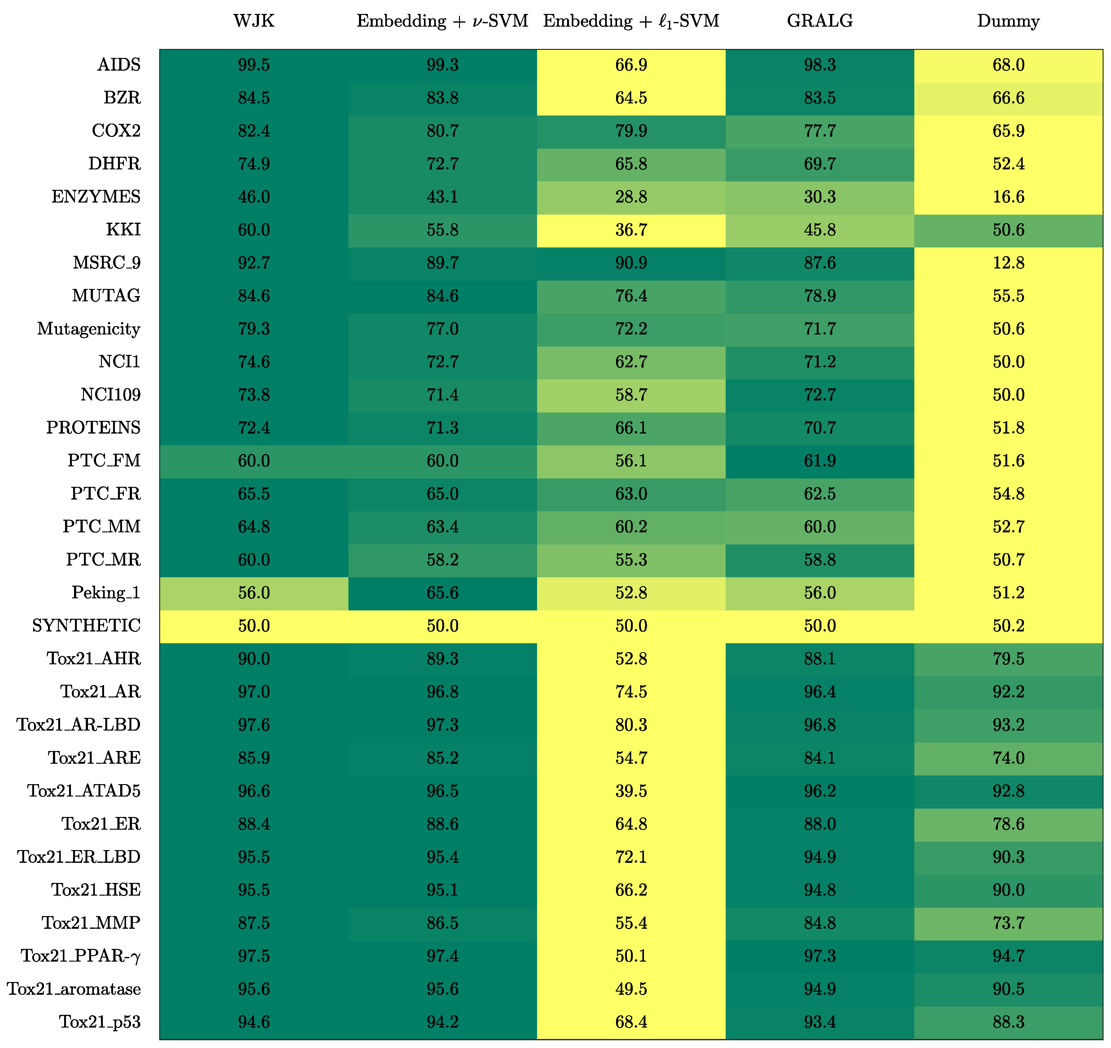
In Figure 1, the accuracy on the test set is shown for the five competitors: the dummy classifier, WJK, GRALG and the proposed embedding procedure using both non-linear -SVM and -SVM. In order to take into account intrinsic randomness in stratified training/test splitting and in genetic optimisation, the results presented here have been averaged across five different runs. Clearly, for the tested datasets, a linear classifier performs poorly: it is indeed well-known that especially for high-dimensional datasets non-linear and linear methods have comparable performances [31,83]. As a matter of fact, for these datasets, Peking_1 leaded to the largest embedding space (approx. 1500 symbols), followed by MSRC_9 (approx. 220 symbols). From Figure 1, it emerges that WJK is generally the best performing method, followed by the proposed embedding procedure with -SVM which is, in turn, followed by GRALG. Indeed, WJK exploits the entire simplicial complexes to the fullest, by considering only simplices belonging to the two simplicial complexes to be matched and without ’discarding’ any simplices due to the explicit (and optimised) embedding procedure, as proposed in this work. Amongst the three methods, WJK is also the fastest to train: the kernel matrix can be pre-evaluated using very fast vectorised statements and the only hyperparameter that needs to be tuned is the -SVM regularisation term, which can done by performing a plain random search in . Amongst the two information granulation-based techniques, the proposed system outperforms GRALG in the vast majority of the cases. This not only has to be imputed to the modelling capabilities offered by hypergraphs but also has a merely computational facet: the number of simple paths is much greater than the number of simplices (A graph with n vertices has paths, whereas the number of cliques goes like ), hence GRALG needs a ’compression stage’ (i.e., a clustering procedure) to return a feasible number of alphabet symbols. This compression stage not only may impact the quality of the embedding procedure, but also leads to training times that are incredibly high with respect to the proposed technique in which simplices can be interpreted as granules themselves.
Another interesting aspect that should be considered for comparison relies on the model interpretability. Despite WJK seems the most appealing technique due to high training efficiency and remarkable generalisation capabilities, it basically relies on pairwise evaluations of a positive-definite kernel function between pair of simplicial complexes which can then be fed into a kernelised classifier. This modus operandi does not make the model interpretable and no knowledge discovery phase can be pursued afterwards. The same is not true for Granular Computing-based pattern recognition systems such as GRALG or the one proposed in this paper, as will be confirmed in Section 4.
3.2. On Real-world Proteomic Data
3.2.1. Experiment #1: Protein Function Classification
Data Retrieval and Preprocessing
The data retrieval process can be summarised as follows:
- the entire Escherichia coli (str. K12) list of proteins has been retrieved from UniProt [84]
- the list has been cross-checked with Protein Data Bank [85] in order to download PDB files for resolved proteins
- proteins with multiple EC numbers have been discarded
- in PDB files containing multiple structure models, only the first model is retained; similarly, for atoms having alternate coordinate locations, only the first location is retained.
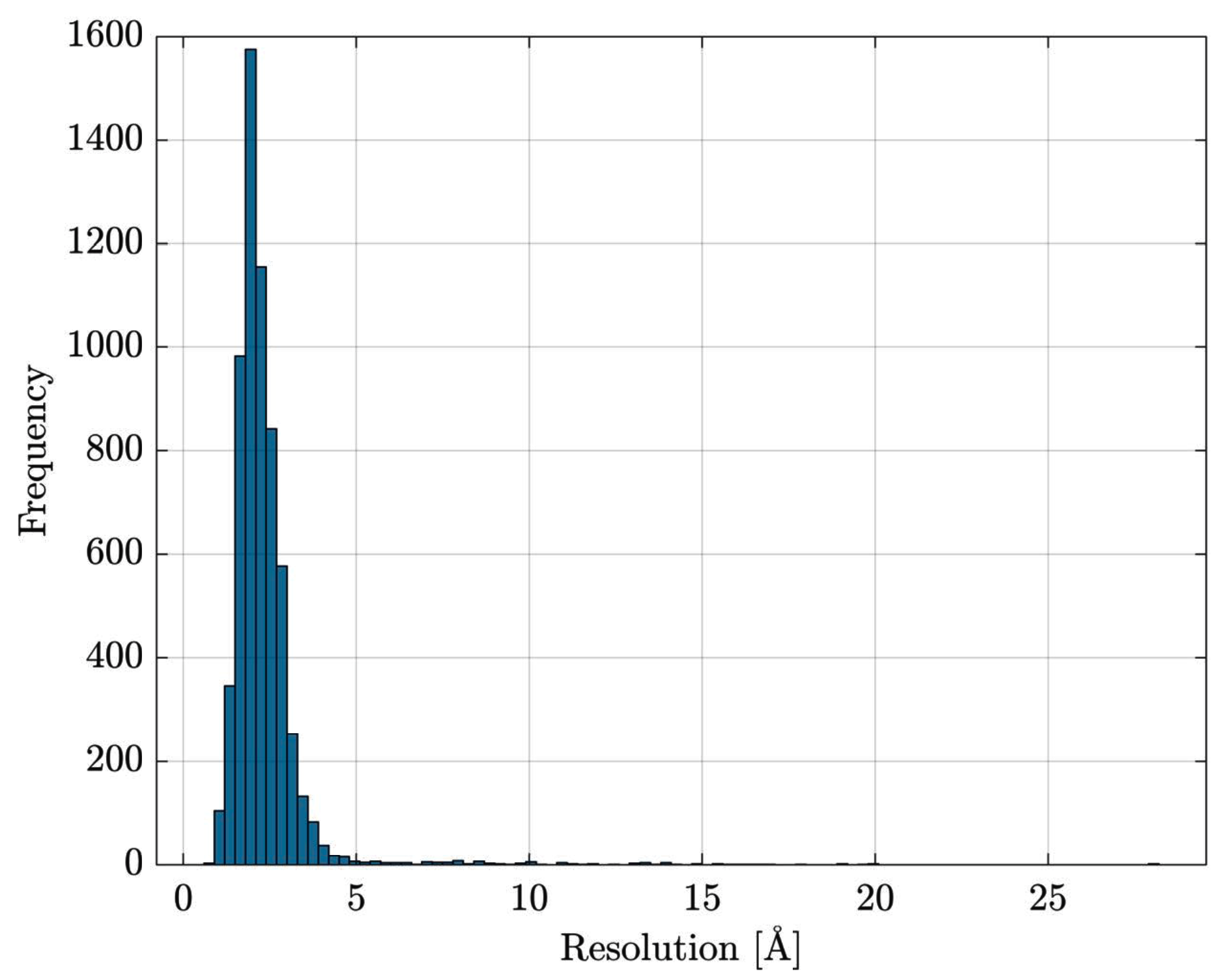
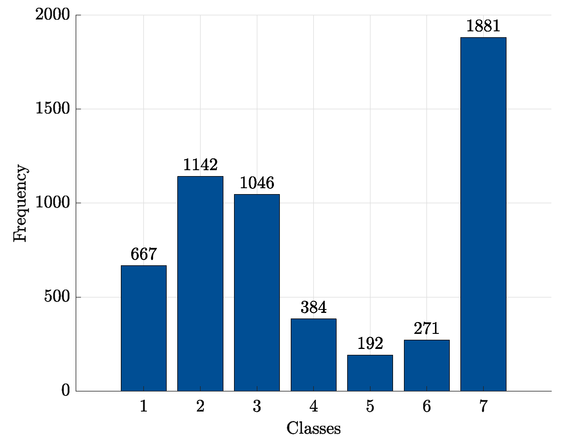
After this retrieval stage, a total number of 6685 proteins has been collected. From this initial set, all proteins without information regarding the measurement resolution have been discarded. Further, in order to consider only good quality structures (i.e., reliable atomic coordinates for building PCNs), all proteins whose measurement resolution is greater than 3Å have been discarded as well. The 3Å threshold has been selected by jointly considering the PCNs connectivity range and the measurement resolution distribution within the dataset (Figure 2). This resolution-based filtering dropped the number of available proteins from 6685 to 5583. The classes distribution is summarised in Figure 3.
Computational Results
For a thorough investigation, this 7-classes problem has been cast into 7 one-against-all binary problems: the ith classifier sees the ith class as positive and all other classes as negatives. In order to take into account the intrinsic random behaviour for both classifiers’ training phases, five stratified training-validation-test sets (Proportions: 50% for training set, 25% for validation set and 25% for test set. The stratified splitting thanks to is performed to preserve labels’ distribution across splits. have been considered and the same splits are fed to both classifiers in order to ensure a fair comparison. Hereafter the average results across these five splits are shown. Again, the Clique complex has been considered in order to build simplicial complexes for PCNs since (by construction) the underlying graph is already available by scoring edges between Å. The resulting alphabet size is reported in Table 1.
Table 2 and Table 3 show the results on the test set for -SVM and -SVM (respectively) with and in the fitness function (13): the former case does not foster any feature selection during training (classifiers can choose as many features as they like), whereas the latter equally optimises performances and sparsity in selecting symbols from the alphabet. The rationale behind using -SVMs alongside -SVMs, despite their poor performances on benchmark data, stems from Section 3; by looking at Table 1 it is clear that this is a properly-said high-dimensional problem (converse to benchmark datasets whose maximum number of features reaches 1500), so it is also worth trying linear methods alongside non-linear ones. Performances on the test set are presented via the following parameters: accuracy (ACC), specificity (SPC), sensitivity (SNS), negative predictive value (NPV) and positive predictive value (PPV), along with the sparsity, defined as percentage of non-zero elements in (or ); that is, the number of selected alphabet symbols over the entire alphabet size: the lower, the better.
From Table 2 it is possible to see that when switching from to , other than selecting a smaller number of symbols, -SVMs tend to improve in terms of SNS and NPV for almost all classes. Similarly, from Table 3, it is possible to see that, when switching from to , -SVMs mainly benefit in terms of feature selection, with only class 7 showing minor performance improvements in terms of SNS and NPV.
By comparing the two classification systems (i.e., by matching Table 2 and Table 3) it is possible to draw the following conclusions:
- at : -SVMs outperform the kernelised counterpart in terms of SNS (all classes) and NPV (all classes), whereas -SVMs outperform the former in terms of SPC (all classes) and PPV (all classes). The overall ACC sees -SVMs outperforming -SVMs only for class 7, the two classifiers perform equally for classes 2 and 4 and for the remaining classes -SVMs perform better. Regardless of which performs the best in an absolute manner, the performance shifts are rather small as far as ACC, SPC and NPV are concerned ( or less), whereas interesting shifts include SNS (-SVMs outperforming by on class 4) and PPV (-SVMs outperforming by on class 3 and on class 5);
- at : -SVMs outperform the kernelised counterpart in terms of SNS (all classes) and NPV (all classes), whereas -SVMs outperform the former in terms of SPC (all classes), PPV (all classes) and ACC (all classes). While the performance shifts are rather small for ACC (≈1–2%) and SPC (), there are remarkable shifts regarding PPV (-SVMs outperform up to for class 5) and SNS (-SVMs outperform up to for class 4).
Conversely, as the sparsity is concerned:
- at : -SVMs select fewer symbols with respect to -SVMs only for classes 1 and 7
- at : -SVMs outperform -SVMs for all classes.
Finally, is also worth stressing that -SVMs are easier to train with respect to the non-linear counterpart for the following reasons: (a) -SVMs, being linear classifiers, do not require the (explicit) kernel evaluation (cf. Equations (10) and (11)); (b) their training consists of solving a Linear Programming optimisation problem (the same is not true for -SVMs, which solve a Quadratic Programming problem); (c) they automatically return a sparse solution, so they only need hyperparameter optimisation (We considered a genetic algorithm for the sake of consistency with -SVMs but lighter procedures can also be pursued for hyperparameter optimisation (e.g., random search or grid search)).
3.2.2. Experiment #2: Protein Solubility Classification
Data Retrieval and Preprocessing
The data retrieval process and be summarised as follows:
- from the eSOL database (eSOL database http://tp-esol.genes.nig.ac.jp/)) developed in the Targeted Proteins Research Project., containing the solubility degree (in percentage) for the E. coli proteins using the chaperone-free PURE system [87], the entire dump has been collected
- proteins with no information about their solubility degree have been discarded
- in order to enlarge the number of samples (From the entire dump, only 432 proteins had their corresponding PDB ID.), we reversed the JW-to-PDB relation by downloading all structure files (if any) related to each JW entry from eSOL. Each structure will inherit the solubility degree from the JW entry
- inconsistent data (e.g., the same PDB with different solubility values) have been discarded; duplicates have been removed in case of redundant data (e.g., one solubility per PDB but multiple JWs)
- proteins that have a solubility degree greater than have been set as . The (small) deviations from can be ascribed to minor experimental errors. After straightforward normalisation, the solubility degree can be considered a real-valued number in range .
This first preprocessing stage leads to a dataset of 5517 proteins. As per the previous experiment, PDB files have been parsed by removing alternate models and alternate atom locations. Finally, proteins with no resolution information or whose resolution is greater than 3Å have been discarded as well. This resolution-based filtering dropped the number of available proteins from 5517 to 4781. The solubility distribution within the resulting dataset is summarised in Figure 4.
Since aim of the classification system is to discriminate between soluble versus non-soluble proteins, a threshold must be set in order to generate categorical output values starting from real-valued solubility degrees. Specifically, all proteins whose solubility degree is greater than will be considered ‘soluble’, whereas the remaining proteins will be considered ‘non-soluble’.
Computational Results
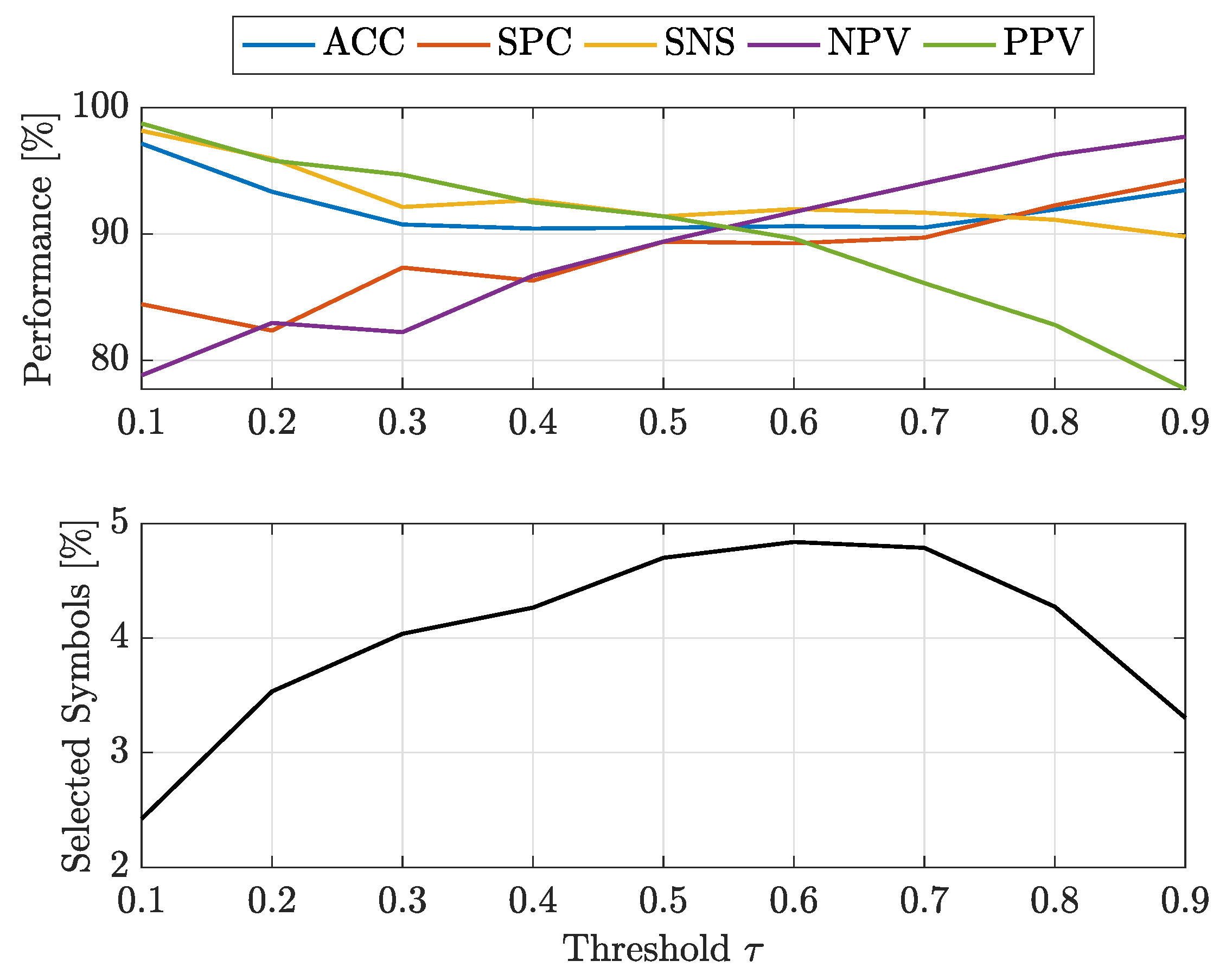
For a thorough investigation, the threshold has been varied from to with step size . For the sake of shorthand, only -SVM has been used for classification since it has been proved successful both in terms of efficiency and effectiveness for the previous PCN experiment.
Figure 5 and Figure 6 show the classification results on test set averaged across five splits for and , respectively. By matching the top plots from Figure 5 and Figure 6, the best threshold values are in range for and for : in the latter case, as , precision (PPV) starts deteriorating. Indeed, for very low threshold values (i.e., ) there will be a lot of ‘soluble’ proteins with respect to the ‘non-soluble’ ones (Many positive instances with respect to the negative ones). Trivially, this is reflected in very high positive-related performance indices (circa ) such as SNS and PPV and rather low negative-related performance indices (circa 80–90%) such as NPV and SPC. The opposite is true for very high thresholds (i.e., ). In the aforementioned ranges, all performance indices are rather balanced: in Figure 5, for , all performance indices are in range 89–94%; in Figure 6, for , all performance indices are in range 89–92%. This (minor) shift in performances is counterbalanced by the number of selected symbols: for approximately of the alphabet symbols have been selected, whereas for the percentage of selected symbols is always below . Interestingly, see Figure 6, the range is also featured by the largest alphabet: a slightly more complex embedding space is needed for maximising the overall performances.
4. Discussion
In order to extract a biochemically relevant explanation from the results of the pattern recognition procedure, for both experiments, we computed over the extracted granules (simplices), namely small peptides located into the protein structure, the main chemico-physical parameters at the amino-acid residue level according to the results presented in Ref. [88]. Each information granule (simplex) has been mapped with 6 real values indicating the average and standard deviation of polarity, volume and hydrophilicity evaluated amongst the amino-acids forming the simplex. The chemico-physical properties of each information granule have been correlated with a score ranging from 1 to 5, namely the number of times said granule has been selected across the five runs: the higher the score, the higher the confidence about its discrimination importance for the classification problem.
Let us discuss the solubility classification problem first. The score assigned to each simplex has been discretised according to the following rules: all scores greater than 2 have been considered ‘positives’, all scores equal to 0 have been considered ‘negatives’ and all other simplices have been discarded. Statistical tests show that, despite the huge number of samples (approx. 11000 simplices), the average volume is not statistically significant (p-value approx. 0.11). This is perfectly coherent if we consider that the volume of a simplex (usually less than 5 residues) is very unlikely to endow biological meaning in terms of the overall protein solubility. On the other hand, the standard deviation volume has been shown to be statistically significant (p-value ). This interesting result shows that simplices composed of ‘similar amino-acids’ (small standard deviation) show better solubility. Nonetheless, it is important to note that, for a given chemico-physical property (e.g., volume in this case) the standard deviation and the average value shall be treated independently and do not show any correlation. This latter aspect of average and standard deviation carrying different information has also been confirmed by analysing the two other properties (polarity and hydrophilicity).
Polarity and hydrophilicity not only show statistical significance (all p-values are less than 0.0001) but also show a strong correlation (>0.99) in terms of both mean values and standard deviations, as shown in Table 4, yet mean values and standard deviations are not correlated with each other (as per the volume case). This perfectly fits with current biochemical knowledge and, specifically, this is consistent with the well-known importance of ‘hydrophobic interaction’ in protein folding (residues with hydrophobicity/hydrophilicity values tend to aggregate [89]).
Similar analyses have been carried for the EC classification problem. All of the seven statistical models show statistical significance, mainly thanks to the large number of samples (more than 12,000 simplices). Table 5 summarises their main characteristics. Alongside the statistical significance, it is interesting to note that all of the seven models have , meaning that they explain 2% of the overall variance.
Furthermore, also in this experiment, hydrophilicity has been shown to be the most important predictor according to linear discriminant analysis [90] and completely superimposable results are obtained for average polarity, which is strictly related to hydrophilicity. Table 6 shows the main characteristics of the seven models where hydrophilicity is concerned and Table 7 is its counterpart as regards polarity. They both report the t-statistics and the relative p-value of the null hypothesis of no contribution of hydrophilicity (polarity) of the multiple linear regression having score for different classes as dependent variable and different chemico-physical indexes relative to the simplices as regressors. As evident, especially hydrophilicity enters a significant contribution to all models as the most important predictor (i.e., the estimated coefficient for average hydrophilicity is approximately one order of magnitude higher with respect to other coefficients). Another interesting aspect is that all models show a negative coefficient for average hydrophilicity and a positive sign for its standard deviation.
In conclusion, beside the confirmation of the pivotal role of residue hydrophilic character in determining the protein structure, it is well known [91] that when shifting from a single residue to an entire protein level, new organisation principles arise and ‘context-dependent’ features largely overcome single residue level properties. The 2% of variance explained is the percentage that can be imputed to the plain chemico-physical properties of individual simplices and one might ask whether the same analyses can be carried out by considering ‘groups of simplices’ instead of individual simplices and scoring their relevance for the problem at hand. This paves the way for new granulation-based studies which should also take into account these aspects. All in all, the observed results confirm the actual biochemical theory, thus providing a ‘lateral validation’ to the pattern recognition procedure, while at the same time pushing biochemists to look for non-local chemico-physical properties for getting rid of protein folding and structure-function relations.
5. Conclusions
Graphs are powerful structures that can capture topological and semantic information from data. However, in many contexts, graphs suffer from the major drawback of having different sizes, hence they cannot be easily compared (e.g., by means of their respective adjacency matrices) and designing a graph-based pattern recognition system is not trivial. In this paper, this problem has been addressed by moving towards an embedding space built on top of simplicial complexes extracted in a fully data-driven manner from the dataset at hand. The embedding procedure follows the symbolic histogram approach, where each pattern is described by the number of occurrences of a given meaningful symbol within the original pattern (graph). In the embedding space any Euclidean classifier can be used, either equipped or not with feature selection capabilities.
Although not mandatory, performing feature selection either by properly choosing the classification system or with the help of optimisation techniques, benefits the model in a two-fold fashion: first, it reduces the embedding space dimension, speeding up the classification of new patterns; second, it improves the model interpretability. Indeed, a major strength of information granulation-based pattern recognition systems is that relevant, meaningful information granules (alphabet symbols) can be analysed by field-experts to derive insights for the problem at hand.
The proposed pattern recognition system has been tested on thirty open-access datasets and benchmarked against two suitable competitors: a kernel method (WJK) which works on simplicial complexes and (by definition) performs an implicit embedding towards an high-dimensional feature space and another information granulation-based classifier (GRALG) which performs explicit embedding but relies on simple paths rather than simplices. Computational results show that the proposed embedding technique outperforms GRALG in almost all of the tested datasets. Albeit WJK seems to be the best performing classification technique, it is noteworthy that no a-posteriori knowledge discovery phase can be performed, whereas the same is not true for information granulation-based classifiers. In order to stress this aspect, we faced two additional real-world problems: the prediction of proteins’ enzymatic class and their solubility. For these problems, along with remarkable classification results, we also investigated some chemico-physical properties related to the amino-acids belonging to the simplices which have been selected as pivotal for the embedding space: statistical analyses confirmed their biological relevance.
A non negligible facet of this work is that the proposed approach is suitable for dealing both with graphs (which can be ’transformed’ into an hypergraph–for example, via Clique complex) and with hypergraphs directly (the embedding procedure indeed relies on simplicial complexes). For the sake of demonstration and testing, graphs have been the major starting point for analysis in order to build simplicial complexes; nonetheless, simplicial complexes can also be evaluated over point clouds (e.g., via Vietoris-Rips complex, Alpha complex). As far as the graph experiments are concerned, an interesting aspect of the proposed technique is that building the embedding space is parameter-free and it can be evaluated in a one-shot fashion: this is true, however, only if the underlying topology is known a-priori and the Clique complex can be used. As other simplicial complexes need to be used (for example, if underlying topology is not available beforehand), the embedding procedure looses its parameter-free peculiarity. Finally, it is worth noting that, in its current implementation, the matching procedure between simplices can be done in an exact manner by considering categorical node labels: future research endeavours can extend the proposed procedure to more complex semantic information on nodes and/or edges.
Author Contributions
Conceptualization, A.M. and A.R.; methodology, A.M. and A.R.; software, A.M.; validation, A.M. and A.G.; investigation, A.M., A.R. and A.G.; data curation, A.M.; writing—original draft preparation, A.M. and A.G.; writing—review and editing, A.M., A.G. and A.R.; supervision A.R..
Funding
This research received no external funding.
Conflicts of Interest
The authors declare no conflict of interest.
Abbreviations
The following abbreviations are used in this manuscript:
| ACC | Accuracy |
| EC | Enzyme Commission |
| NPV | Negative Predictive Value |
| PCN | Protein Contact Network |
| PDB | Protein Data Bank |
| PPV | Positive Predictive Value |
| SNS | Sensitivity |
| SPC | Specificity |
| SVM | Support Vector Machine |
References
- Giuliani, A.; Filippi, S.; Bertolaso, M. Why network approach can promote a new way of thinking in biology. Front. Genet. 2014, 5, 83. [Google Scholar] [CrossRef] [PubMed]
- Di Paola, L.; De Ruvo, M.; Paci, P.; Santoni, D.; Giuliani, A. Protein contact networks: An emerging paradigm in chemistry. Chem. Rev. 2012, 113, 1598–1613. [Google Scholar] [CrossRef] [PubMed]
- Krishnan, A.; Zbilut, J.P.; Tomita, M.; Giuliani, A. Proteins as networks: Usefulness of graph theory in protein science. Curr. Protein Pept. Sci. 2008, 9, 28–38. [Google Scholar] [CrossRef] [PubMed]
- Jeong, H.; Tombor, B.; Albert, R.; Oltvai, Z.N.; Barabási, A.L. The large-scale organization of metabolic networks. Nature 2000, 407, 651. [Google Scholar] [CrossRef]
- Di Paola, L.; Giuliani, A. Protein–Protein Interactions: The Structural Foundation of Life Complexity. In Encyclopedia of Life Sciences (eLS); John Wiley & Sons: Chichester, UK, 2017; pp. 1–12. [Google Scholar] [CrossRef]
- Wuchty, S. Scale-Free Behavior in Protein Domain Networks. Mol. Biol. Evol. 2001, 18, 1694–1702. [Google Scholar] [CrossRef] [Green Version]
- Davidson, E.H.; Rast, J.P.; Oliveri, P.; Ransick, A.; Calestani, C.; Yuh, C.H.; Minokawa, T.; Amore, G.; Hinman, V.; Arenas-Mena, C.; et al. A Genomic Regulatory Network for Development. Science 2002, 295, 1669–1678. [Google Scholar] [CrossRef] [Green Version]
- Gasteiger, J.; Engel, T. Chemoinformatics: A Textbook; John Wiley & Sons: Haboken, NJ, USA, 2006. [Google Scholar]
- Wasserman, S.; Faust, K. Social Network Analysis: Methods and Applications; Cambridge University Press: New York, NJ, USA, 1994. [Google Scholar]
- Deutsch, A.; Fernandez, M.; Florescu, D.; Levy, A.; Suciu, D. A query language for XML. Comput. Netw. 1999, 31, 1155–1169. [Google Scholar] [CrossRef]
- Weis, M.; Naumann, F. Detecting Duplicates in Complex XML Data. In Proceedings of the 22nd International Conference on Data Engineering (ICDE’06), Atlanta, GA, USA, 3–7 April 2006; p. 109. [Google Scholar] [CrossRef]
- Collins, M.; Duffy, N. Convolution Kernels for Natural Language. In Proceedings of the 14th International Conference on Neural Information Processing Systems: Natural and Synthetic (NIPS’01), Vancouver, BC, Canada, 3–8 December 2001; MIT Press: Cambridge, MA, USA, 2001; pp. 625–632. [Google Scholar]
- Das, N.; Ghosh, S.; Gonçalves, T.; Quaresma, P. Comparison of Different Graph Distance Metrics for Semantic Text Based Classification. Polibits 2014, 51–58. [Google Scholar] [CrossRef]
- Das, N.; Ghosh, S.; Gonçalves, T.; Quaresma, P. Using Graphs and Semantic Information to Improve Text Classifiers. In Advances in Natural Language Processing; Przepiórkowski, A., Ogrodniczuk, M., Eds.; Springer: Cham, Switzerland, 2014; pp. 324–336. [Google Scholar] [CrossRef]
- Livi, L.; Rizzi, A.; Sadeghian, A. Granular modeling and computing approaches for intelligent analysis of non-geometric data. Appl. Soft Comput. 2015, 27, 567–574. [Google Scholar] [CrossRef]
- Livi, L.; Sadeghian, A. Granular computing, computational intelligence, and the analysis of non-geometric input spaces. Granul. Comput. 2016, 1, 13–20. [Google Scholar] [CrossRef]
- Martino, A.; Giuliani, A.; Rizzi, A. Granular Computing Techniques for Bioinformatics Pattern Recognition Problems in Non-metric Spaces. In Computational Intelligence for Pattern Recognition; Pedrycz, W., Chen, S.M., Eds.; Springer: Cham, Switzerland, 2018; pp. 53–81. [Google Scholar] [CrossRef]
- Pękalska, E.; Duin, R.P. The Dissimilarity Representation for Pattern Recognition: Foundations and Applications; World Scientific: Singapore, 2005. [Google Scholar] [CrossRef]
- Livi, L.; Rizzi, A. Graph ambiguity. Fuzzy Sets Syst. 2013, 221, 24–47. [Google Scholar] [CrossRef] [Green Version]
- Livi, L.; Rizzi, A. The graph matching problem. Pattern Anal. Appl. 2013, 16, 253–283. [Google Scholar] [CrossRef]
- Neuhaus, M.; Bunke, H. Bridging the Gap between Graph Edit Distance and Kernel Machines; World Scientific: Singapore, 2007. [Google Scholar] [CrossRef]
- Cinti, A.; Bianchi, F.M.; Martino, A.; Rizzi, A. A Novel Algorithm for Online Inexact String Matching and its FPGA Implementation. Cognit. Comput. 2019. [Google Scholar] [CrossRef]
- Pękalska, E.; Duin, R.P.; Paclík, P. Prototype selection for dissimilarity-based classifiers. Pattern Recognit. 2006, 39, 189–208. [Google Scholar] [CrossRef]
- Livi, L.; Rizzi, A.; Sadeghian, A. Optimized dissimilarity space embedding for labeled graphs. Inf. Sci. 2014, 266, 47–64. [Google Scholar] [CrossRef]
- De Santis, E.; Martino, A.; Rizzi, A.; Frattale Mascioli, F.M. Dissimilarity Space Representations and Automatic Feature Selection for Protein Function Prediction. In Proceedings of the 2018 International Joint Conference on Neural Networks (IJCNN), Rio de Janeiro, Brazil, 8–13 July 2018; pp. 1–8. [Google Scholar] [CrossRef]
- Martino, A.; De Santis, E.; Giuliani, A.; Rizzi, A. Modelling and Recognition of Protein Contact Networks by Multiple Kernel Learning and Dissimilarity Representations. Inf. Sci. 2019. Under Review. [Google Scholar]
- Shawe-Taylor, J.; Cristianini, N. Kernel Methods for Pattern Analysis; Cambridge University Press: Cambridge, UK, 2004. [Google Scholar] [CrossRef]
- Schölkopf, B.; Smola, A.J. Learning with Kernels: Support Vector Machines, Regularization, Optimization, and Beyond; MIT Press: Massachusetts, MA, USA, 2002. [Google Scholar]
- Cristianini, N.; Shawe-Taylor, J. An Introduction to Support Vector Machines and Other Kernel-Based Learning Methods; Cambridge University Press: Cambridge, MA, USA, 2000. [Google Scholar] [CrossRef]
- Mercer, J. Functions of positive and negative type, and their connection with the theory of integral equations. Philos. Trans. R. Soc. Lond. Ser. A Contain. Pap. A Math. Phys. Character 1909, 209, 415–446. [Google Scholar] [CrossRef]
- Cover, T.M. Geometrical and statistical properties of systems of linear inequalities with applications in pattern recognition. IEEE Trans. Electron. Comput. 1965, 326–334. [Google Scholar] [CrossRef]
- Li, J.B.; Chu, S.C.; Pan, J.S. Kernel Learning Algorithms for Face Recognition; Springer: New York, NY, USA, 2014. [Google Scholar]
- Bargiela, A.; Pedrycz, W. Granular Computing: An Introduction; Kluwer Academic Publishers: Boston, MA, USA, 2003. [Google Scholar]
- Pedrycz, W.; Skowron, A.; Kreinovich, V. Handbook of Granular Computing; John Wiley & Sons: Haboken, NJ, USA, 2008. [Google Scholar]
- Pedrycz, W.; Homenda, W. Building the fundamentals of granular computing: A principle of justifiable granularity. Appl. Soft Comput. 2013, 13, 4209–4218. [Google Scholar] [CrossRef]
- Yao, Y.; Zhao, L. A measurement theory view on the granularity of partitions. Inf. Sci. 2012, 213, 1–13. [Google Scholar] [CrossRef]
- Yang, J.; Wang, G.; Zhang, Q. Knowledge distance measure in multigranulation spaces of fuzzy equivalence relations. Inf. Sci. 2018, 448, 18–35. [Google Scholar] [CrossRef]
- Ding, S.; Du, M.; Zhu, H. Survey on granularity clustering. Cognit. Neurodyn. 2015, 9, 561–572. [Google Scholar] [CrossRef] [PubMed] [Green Version]
- Martino, A.; Rizzi, A.; Frattale Mascioli, F.M. Efficient Approaches for Solving the Large-Scale k-medoids Problem. In Proceedings of the 9th International Joint Conference on Computational Intelligence—Volume 1: IJCCI; SciTePress: Setúbal, Portugal, 2017; pp. 338–347. [Google Scholar] [CrossRef]
- Del Vescovo, G.; Livi, L.; Frattale Mascioli, F.M.; Rizzi, A. On the problem of modeling structured data with the MinSOD representative. Int. J. Comput. Theory Eng. 2014, 6, 9. [Google Scholar] [CrossRef]
- Martino, A.; Rizzi, A.; Frattale Mascioli, F.M. Efficient Approaches for Solving the Large-Scale k-Medoids Problem: Towards Structured Data. In Computational Intelligence, Proceedings of the 9th International Joint Conference, IJCCI 2017, Funchal-Madeira, Portugal, 1–3 November 2017; Revised Selected Papers; Sabourin, C., Merelo, J.J., Madani, K., Warwick, K., Eds.; Springer: Cham, Switzerland, 2019; pp. 199–219. [Google Scholar] [CrossRef]
- Martino, A.; Rizzi, A.; Frattale Mascioli, F.M. Distance Matrix Pre-Caching and Distributed Computation of Internal Validation Indices in k-medoids Clustering. In Proceedings of the 2018 International Joint Conference on Neural Networks (IJCNN), Rio de Janeiro, Brazil, 8–13 July 2018; pp. 1–8. [Google Scholar] [CrossRef]
- Bianchi, F.M.; Livi, L.; Rizzi, A.; Sadeghian, A. A Granular Computing approach to the design of optimized graph classification systems. Soft Comput. 2014, 18, 393–412. [Google Scholar] [CrossRef]
- Bianchi, F.M.; Scardapane, S.; Rizzi, A.; Uncini, A.; Sadeghian, A. Granular Computing Techniques for Classification and Semantic Characterization of Structured Data. Cognit. Comput. 2016, 8, 442–461. [Google Scholar] [CrossRef]
- Singh, P.K. Similar Vague Concepts Selection Using Their Euclidean Distance at Different Granulation. Cognit. Comput. 2018, 10, 228–241. [Google Scholar] [CrossRef]
- Del Vescovo, G.; Rizzi, A. Automatic classification of graphs by symbolic histograms. In Proceedings of the 2007 IEEE International Conference on Granular Computing (GRC 2007), Fremont, CA, USA, 2–4 November 2007; p. 410. [Google Scholar] [CrossRef]
- Rizzi, A.; Del Vescovo, G.; Livi, L.; Frattale Mascioli, F.M. A new Granular Computing approach for sequences representation and classification. Proceedings ot the 2012 International Joint Conference on Neural Networks (IJCNN), Brisbane, QLD, Australia, 10–15 June 2012; pp. 1–8. [Google Scholar] [CrossRef]
- Horak, D.; Maletić, S.; Rajković, M. Persistent homology of complex networks. J. Stat. Mech. Theory Exp. 2009, 2009, P03034. [Google Scholar] [CrossRef]
- Estrada, E.; Rodriguez-Velazquez, J.A. Complex networks as hypergraphs. arXiv 2005, arXiv:physics/0505137. [Google Scholar]
- Carlsson, G. Topology and data. Bull. Am. Math. Soc. 2009, 46, 255–308. [Google Scholar] [CrossRef] [Green Version]
- Wasserman, L. Topological Data Analysis. Annu. Rev. Stat. Its Appl. 2018, 5, 501–532. [Google Scholar] [CrossRef] [Green Version]
- Ramadan, E.; Tarafdar, A.; Pothen, A. A hypergraph model for the yeast protein complex network. In Proceedings of the 18th International Parallel and Distributed Processing Symposium, Santa Fe, NM, USA, 26–30 April 2004; p. 189. [Google Scholar] [CrossRef]
- Gaudelet, T.; Malod-Dognin, N.; Pržulj, N. Higher-order molecular organization as a source of biological function. Bioinformatics 2018, 34, i944–i953. [Google Scholar] [CrossRef] [PubMed]
- Malod-Dognin, N.; Pržulj, N. Functional geometry of protein-protein interaction networks. arXiv 2018, arXiv:1804.04428. [Google Scholar]
- Barbarossa, S.; Sardellitti, S. Topological Signal Processing over Simplicial Complexes. arXiv 2019, arXiv:1907.11577. [Google Scholar]
- Barbarossa, S.; Tsitsvero, M. An introduction to hypergraph signal processing. In Proceedings of the IEEE International Conference on Acoustics, Speech and Signal Processing (ICASSP), Shanghai, China, 20–25 March 2016; pp. 6425–6429. [Google Scholar] [CrossRef]
- Barbarossa, S.; Sardellitti, S.; Ceci, E. Learning from signals defined over simplicial complexes. In Proceedings of the 2018 IEEE Data Science Workshop (DSW), Lausanne, Switzerland, 4–6 June 2018; pp. 51–55. [Google Scholar] [CrossRef]
- Berge, C. Graphs and Hypergraphs; Elsevier: Oxford, UK, 1973. [Google Scholar]
- Zomorodian, A. Topological data analysis. Adv. Appl. Comput. Topol. 2012, 70, 1–39. [Google Scholar] [Green Version]
- Ghrist, R.W. Elementary Applied Topology; Createspace: Seattle, WA, USA, 2014. [Google Scholar]
- Hausmann, J.C. On the Vietoris-Rips complexes and a cohomology theory for metric spaces. Ann. Math. Stud. 1995, 138, 175–188. [Google Scholar]
- Zomorodian, A. Fast construction of the Vietoris-Rips complex. Comput. Graph. 2010, 34, 263–271. [Google Scholar] [CrossRef]
- Bandelt, H.J.; Chepoi, V. Metric graph theory and geometry: A survey. Contemp. Math. 2008, 453, 49–86. [Google Scholar]
- Bandelt, H.J.; Prisner, E. Clique graphs and Helly graphs. J. Comb. Theory Ser. B 1991, 51, 34–45. [Google Scholar] [CrossRef] [Green Version]
- Giusti, C.; Ghrist, R.; Bassett, D.S. Two’s company, three (or more) is a simplex. J. Comput. Neurosci. 2016, 41, 1–14. [Google Scholar] [CrossRef]
- Zomorodian, A.; Carlsson, G. Computing persistent homology. Discret. Comput. Geom. 2005, 33, 249–274. [Google Scholar] [CrossRef]
- Martino, A.; Rizzi, A.; Frattale Mascioli, F.M. Supervised Approaches for Protein Function Prediction by Topological Data Analysis. In Proceedings of the 2018 International Joint Conference on Neural Networks (IJCNN), Rio de Janeiro, Brazil, 8–13 July 2018; pp. 1–8. [Google Scholar] [CrossRef]
- Bron, C.; Kerbosch, J. Algorithm 457: Finding All Cliques of an Undirected Graph. Commun. ACM 1973, 16, 575–577. [Google Scholar] [CrossRef]
- Cazals, F.; Karande, C. A note on the problem of reporting maximal cliques. Theor. Comput. Sci. 2008, 407, 564–568. [Google Scholar] [CrossRef] [Green Version]
- Tomita, E.; Tanaka, A.; Takahashi, H. The worst-case time complexity for generating all maximal cliques and computational experiments. Theor. Comput. Sci. 2006, 363, 28–42. [Google Scholar] [CrossRef] [Green Version]
- Goldberg, D.E. Genetic Algorithms in Search, Optimization and Machine Learning, 1st ed.; Addison-Wesley Longman Publishing Co., Inc.: Boston, MA, USA, 1989. [Google Scholar]
- Schölkopf, B.; Smola, A.J.; Williamson, R.C.; Bartlett, P.L. New support vector algorithms. Neural Comput. 2000, 12, 1207–1245. [Google Scholar] [CrossRef]
- Zhu, J.; Rosset, S.; Tibshirani, R.; Hastie, T.J. 1-norm support vector machines. In Proceedings of the 16th International Conference on Neural Information Processing Systems, Whistler, BC, Canada, 9–11 December 2003; pp. 49–56. [Google Scholar]
- Boser, B.E.; Guyon, I.; Vapnik, V. A training algorithm for optimal margin classifiers. In Proceedings of the Fifth Annual Workshop on Computational Learning Theory, Pittsburgh, PA, USA, 27–29 July 1992; pp. 144–152. [Google Scholar]
- Cortes, C.; Vapnik, V. Support-vector networks. Mach. Learn. 1995, 20, 273–297. [Google Scholar] [CrossRef]
- Powers, D.M.W. Evaluation: From precision, recall and f-measure to roc., informedness, markedness & correlation. J. Mach. Learn. Technol. 2011, 2, 37–63. [Google Scholar]
- Youden, W.J. Index for rating diagnostic tests. Cancer 1950, 3, 32–35. [Google Scholar] [CrossRef]
- Martino, A.; Rizzi, A. (Hyper)Graph Kernels over Simplicial Complexes. Pattern Recognit. 2019. Under Review. [Google Scholar]
- Bianchi, F.M.; Scardapane, S.; Livi, L.; Uncini, A.; Rizzi, A. An interpretable graph-based image classifier. In Proceedings of the 2014 International Joint Conference on Neural Networks (IJCNN), Beijing, China, 6–11 July 2014; pp. 2339–2346. [Google Scholar] [CrossRef]
- Baldini, L.; Martino, A.; Rizzi, A. Stochastic Information Granules Extraction for Graph Embedding and Classification. In Proceedings of the 11th International Joint Conference on Computational Intelligence—Volume 1: NCTA; SciTePress: Vienna, Austria, 2019; pp. 391–402. [Google Scholar] [CrossRef]
- Kersting, K.; Kriege, N.M.; Morris, C.; Mutzel, P.; Neumann, M. Benchmark Data Sets for Graph Kernels. 2016. Available online: http://graphkernels.cs.tu-dortmund.de (accessed on 26 September 2019).
- Di Noia, A.; Martino, A.; Montanari, P.; Rizzi, A. Supervised machine learning techniques and genetic optimization for occupational diseases risk prediction. Soft Comput. 2019. [Google Scholar] [CrossRef]
- Fan, R.E.; Chang, K.W.; Hsieh, C.J.; Wang, X.R.; Lin, C.J. LIBLINEAR: A library for large linear classification. J. Mach. Learn. Res. 2008, 9, 1871–1874. [Google Scholar]
- The UniProt Consortium. UniProt: The universal protein knowledgebase. Nucleic Acids Res. 2017, 45, D158–D169. [Google Scholar] [CrossRef] [PubMed]
- Berman, H.M.; Westbrook, J.; Feng, Z.; Gilliland, G.; Bhat, T.N.; Weissig, H.; Shindyalov, I.N.; Bourne, P.E. The Protein Data Bank. Nucleic Acids Res. 2000, 28, 235–242. [Google Scholar] [CrossRef] [PubMed] [Green Version]
- Martino, A.; Maiorino, E.; Giuliani, A.; Giampieri, M.; Rizzi, A. Supervised Approaches for Function Prediction of Proteins Contact Networks from Topological Structure Information. In Image Analysis, Proceedings of the 20th Scandinavian Conference, Tromsø, Norway, 12–14 June 2017; Sharma, P., Bianchi, F.M., Eds.; Part I; Springer: Cham, Switzerland, 2017; pp. 285–296. [Google Scholar] [CrossRef]
- Shimizu, Y.; Inoue, A.; Tomari, Y.; Suzuki, T.; Yokogawa, T.; Nishikawa, K.; Ueda, T. Cell-free translation reconstituted with purified components. Nat. Biotechnol. 2001, 19, 751. [Google Scholar] [CrossRef] [PubMed]
- Barley, M.H.; Turner, N.J.; Goodacre, R. Improved descriptors for the quantitative structure–activity relationship modeling of peptides and proteins. J. Chem. Inf. Model. 2018, 58, 234–243. [Google Scholar] [CrossRef] [PubMed]
- Nayar, D.; van der Vegt, N.F.A. Cosolvent effects on polymer hydration drive hydrophobic collapse. J. Phys. Chem. B 2018, 122, 3587–3595. [Google Scholar] [CrossRef] [PubMed]
- Fisher, R.A. The statistical utilization of multiple measurements. Ann. Eugen. 1938, 8, 376–386. [Google Scholar] [CrossRef]
- Colafranceschi, M.; Colosimo, A.; Zbilut, J.P.; Uversky, V.N.; Giuliani, A. Structure-related statistical singularities along protein sequences: A correlation study. J. Chem. Inf. Model. 2005, 45, 183–189. [Google Scholar] [CrossRef] [PubMed]
Figure 1.
Average accuracy on the test set amongst the dummy classifier, GRALG, WJK and the proposed embedding technique. Results are given in percentage. The colour scale has been normalised row-wise (i.e., for each dataset) from yellow (lower values) towards green (higher values, preferred).
Figure 1.
Average accuracy on the test set amongst the dummy classifier, GRALG, WJK and the proposed embedding technique. Results are given in percentage. The colour scale has been normalised row-wise (i.e., for each dataset) from yellow (lower values) towards green (higher values, preferred).

Figure 2.
Resolution distribution within the initial 6685 proteins set. Proteins with no resolution information are not considered.
Figure 2.
Resolution distribution within the initial 6685 proteins set. Proteins with no resolution information are not considered.

Figure 3.
Classes distribution within the final 5583 proteins set.

Figure 4.
Solubility distribution within the final 4781 proteins set.

Figure 5.
Average Performance on Test Set for Experiment #2 (-SVM, ).

Figure 6.
Average Performance on Test Set for Experiment #2 (-SVM, ).


Table 1.
Alphabet size (mean ± standard deviation).
| Class | ||||||
|---|---|---|---|---|---|---|
| 1 | 2 | 3 | 4 | 5 | 6 | 7 |
Table 2.
Average results (in percentage) on Test Set for -SVM. In bold, the best between the two fitness function tradeoff values for .
Table 2.
Average results (in percentage) on Test Set for -SVM. In bold, the best between the two fitness function tradeoff values for .
| Class | ACC | SPC | SNS | NPV | PPV | Sparsity | |
|---|---|---|---|---|---|---|---|
| 1 | 0.5 | 95.3 | 96.5 | 87.1 | 98.2 | 77.7 | 3.3 |
| 1 | 97 | 98.4 | 87.3 | 98.3 | 88 | 16 | |
| 2 | 0.5 | 92.7 | 94.2 | 86.7 | 96.5 | 79.6 | 4.5 |
| 1 | 94.5 | 97.3 | 83.8 | 95.9 | 88.9 | 22.7 | |
| 3 | 0.5 | 92.1 | 93.8 | 84.4 | 96.3 | 76.2 | 4 |
| 1 | 93.3 | 95.5 | 83.9 | 96.3 | 81.9 | 17.4 | |
| 4 | 0.5 | 96.6 | 97.7 | 82.5 | 98.7 | 72.9 | 2.8 |
| 1 | 97.3 | 98.6 | 79.8 | 98.5 | 81.6 | 7.8 | |
| 5 | 0.5 | 96.9 | 97.8 | 71.7 | 99 | 56.9 | 1.8 |
| 1 | 97.9 | 98.9 | 70.4 | 98.9 | 75.3 | 5.1 | |
| 6 | 0.5 | 97.5 | 97.9 | 88.8 | 99.4 | 71.5 | 2.2 |
| 1 | 98.7 | 99.4 | 86.2 | 99.3 | 87.8 | 9.6 | |
| 7 | 0.5 | 86.6 | 89.9 | 80.1 | 89.9 | 80.5 | 4.8 |
| 1 | 88.8 | 91.6 | 83.4 | 91.6 | 83.6 | 36.3 |
Table 3.
Average results (in percentage) on Test Set for -SVM. In bold, the best between the two fitness function tradeoff values for .
Table 3.
Average results (in percentage) on Test Set for -SVM. In bold, the best between the two fitness function tradeoff values for .
| Class | ACC | SPC | SNS | NPV | PPV | Sparsity | |
|---|---|---|---|---|---|---|---|
| 1 | 0.5 | 96.8 | 99 | 80.4 | 97.4 | 92 | 9.9 |
| 1 | 97.2 | 99.2 | 81.9 | 97.6 | 93.6 | 11.5 | |
| 2 | 0.5 | 93.9 | 98 | 77.8 | 94.5 | 90.9 | 6.8 |
| 1 | 94.5 | 98.3 | 79.7 | 95 | 92.2 | 26.1 | |
| 3 | 0.5 | 94 | 98.5 | 74.3 | 94.3 | 92.1 | 6.8 |
| 1 | 94.7 | 98.5 | 78.2 | 95.1 | 92.3 | 18.6 | |
| 4 | 0.5 | 97.3 | 99.3 | 69.6 | 97.8 | 88.4 | 12.8 |
| 1 | 97.3 | 99.4 | 69.2 | 97.8 | 89.9 | 19.1 | |
| 5 | 0.5 | 98.5 | 99.8 | 61.3 | 98.6 | 93 | 13.6 |
| 1 | 98.7 | 99.9 | 63.8 | 98.7 | 97.1 | 31.7 | |
| 6 | 0.5 | 98.9 | 99.9 | 80.3 | 99 | 97.1 | 23.3 |
| 1 | 99.1 | 99.9 | 83.5 | 99.2 | 97.2 | 28.7 | |
| 7 | 0.5 | 87.4 | 93 | 76.5 | 88.6 | 84.7 | 6.5 |
| 1 | 87.4 | 93.4 | 75.7 | 88.3 | 85.3 | 6.9 |
Table 4.
Pearson correlation coefficients between polarity and hydrophilicity.
| Polarity (avg) | Hydrophilicity (avg) | Polarity (std) | Hydrophilicity (std) | |
|---|---|---|---|---|
| Polarity (avg) | 1 | 0.99818 | −0.01869 | −0.06879 |
| Hydrophilicity (avg) | 0.99818 | 1 | −0.03705 | −0.08582 |
| Polarity (std) | −0.01869 | −0.03705 | 1 | 0.99397 |
| Hydrophilicity (std) | −0.06879 | −0.08582 | 0.99397 | 1 |
Table 5.
Variance explained and statistical significance for the seven models.
| EC1 | EC2 | EC3 | EC4 | EC5 | EC6 | Not Enzymes | |
|---|---|---|---|---|---|---|---|
| 0.0250 | 0.0239 | 0.0212 | 0.0199 | 0.0239 | 0.0170 | 0.0250 | |
| p | <0.0001 | <0.0001 | <0.0001 | <0.0001 | <0.0001 | <0.0001 | <0.0001 |
Table 6.
Hydrophilicity contribution to score for different classes.
| Hydrophilicity (avg) | Hydrophilicity (std) | |||||
|---|---|---|---|---|---|---|
| Class | t-Value | p | Coefficient | t-Value | p | Coefficient |
| 1 | 11.55 | <0.0001 | −4.17734 | 0.92 | 0.3563 | 0.24438 |
| 2 | 10.52 | <0.0001 | −3.73211 | 0.0647 | 1.85 | 0.47999 |
| 3 | 10.61 | <0.0001 | −3.38981 | 0.0651 | 1.84 | 0.43182 |
| 4 | 11.08 | <0.0001 | −2.98596 | 2.11 | 0.0352 | 0.41574 |
| 5 | 12.13 | <0.0001 | −2.43624 | 2.49 | 0.0127 | 0.36671 |
| 6 | 10.73 | <0.0001 | −2.65512 | 2.57 | 0.01 | 0.46672 |
| 7 | 11.55 | <0.0001 | −4.17734 | 0.92 | 0.3563 | 0.24438 |
Table 7.
Polarity contribution to score for different classes.
| Polarity (avg) | Polarity (std) | |||||
|---|---|---|---|---|---|---|
| Class | t-Value | p | Coefficient | t-Value | p | Coefficient |
| 1 | 11.27 | <0.0001 | 1.51515 | 1.77 | 0.0762 | −0.17376 |
| 2 | 10.26 | <0.0001 | 1.35280 | 2.52 | 0.0118 | −0.24206 |
| 3 | 10.43 | <0.0001 | 1.23898 | 2.62 | 0.0089 | −0.22655 |
| 4 | 10.83 | <0.0001 | 1.08515 | 2.72 | 0.0066 | −0.19836 |
| 5 | 11.84 | <0.0001 | 0.88388 | 3.16 | 0.0016 | −0.17190 |
| 6 | 10.52 | <0.0001 | 0.96768 | 3.14 | 0.0017 | −0.21080 |
| 7 | 11.27 | <0.0001 | 1.51515 | 1.77 | 0.0762 | −0.17376 |
© 2019 by the authors. Licensee MDPI, Basel, Switzerland. This article is an open access article distributed under the terms and conditions of the Creative Commons Attribution (CC BY) license (http://creativecommons.org/licenses/by/4.0/).
Share and Cite
MDPI and ACS Style
Martino, A.; Giuliani, A.; Rizzi, A. (Hyper)Graph Embedding and Classification via Simplicial Complexes. Algorithms 2019, 12, 223. https://0-doi-org.brum.beds.ac.uk/10.3390/a12110223
AMA Style
Martino A, Giuliani A, Rizzi A. (Hyper)Graph Embedding and Classification via Simplicial Complexes. Algorithms. 2019; 12(11):223. https://0-doi-org.brum.beds.ac.uk/10.3390/a12110223
Chicago/Turabian StyleMartino, Alessio, Alessandro Giuliani, and Antonello Rizzi. 2019. "(Hyper)Graph Embedding and Classification via Simplicial Complexes" Algorithms 12, no. 11: 223. https://0-doi-org.brum.beds.ac.uk/10.3390/a12110223
Note that from the first issue of 2016, this journal uses article numbers instead of page numbers. See further details here.