Multiple-Attribute Decision Making ELECTRE II Method under Bipolar Fuzzy Model

Abstract

The core aim of this paper is to provide a new multiple-criteria decision making (MCDM) model, namely bipolar fuzzy ELimination and Choice Translating REality (ELECTRE) II method, by combining the bipolar fuzzy set with ELECTRE II technique. It can be used to solve the problems having bipolar uncertainty. The proposed method is established by defining the concept of bipolar fuzzy strong, median and weak concordance as well as discordance sets and indifferent set to define two types of outranking relations, namely strong outranking relation and weak outranking relation. The normalized weights of criteria, which may be partly or completely unknown for decision makers, are calculated by using an optimization technique, which is based on maximizing deviation method. A systematic iterative procedure is applied to strongly outrank as well as weakly outrank graphs to determine the ranking of favorable actions or alternatives or to choose the best possible solution. The implementation of the proposed method is presented by numerical examples such as selection of business location and to chose the best supplier. A comparative analysis of proposed ELECTRE II method is also presented with already existing multiple-attribute decision making methods, including Technique for the Order of Preference by Similarity to an Ideal Solution (TOPSIS) and ELECTRE I under bipolar fuzzy environment by solving the problem of business location.

1. Introduction

Multiple-criteria decision making (MCDM) techniques are concerned with designing and evaluating the structure of decision and planning problems involving multiple criteria. These models accommodate the procedure of determining the most convenient option among the reasonable alternatives and have a great role in cost minimization, time saving and accumulating accurate decisions. MCDM models are established on the basis of variations of beliefs regarding to decision maker’s choice and utilize a particular type of preference intelligence system. The decision making problems in different fields including economics, business management, information technology, social sciences and medical sciences are structured and solved using different MCDM models. MCDM based systematic approach has seen an excessive amount of use over the last several decades and a variety of MCDM models containing Analytic Hierarchy Process (AHP) [1], Technique for the Order of Preference by Similarity to an Ideal Solution(TOPSIS) [2], VIekriterijumsko KOmpromisno Rangiranje (VIKOR) meaning multi-criteria optimization and compromise solution [3], ELimination and Choice Translating REality (ELECTRE) [4] and Preference Ranking Organization Method for Enrichment of Evaluations (PROMETHEE) [5] have been presented to rank alternatives or to find the kernel solution. In classical MCDM methods, the preference ratings of alternatives with respect to criteria and the attribute weights are given in the form of precise information or data. To cope with such type of problems having ambiguous information and imprecise in knowledge, Bellman and Zadeh [6] in 1970 introduced the decision making model for an uncertain system using the concept of fuzzy sets. Since then, the decision making using fuzzy sets has become an interesting field of research for practitioners. A series of outranking methods is used to rank a set of alternatives. The ELECTRE method as well as its derivatives has a significant role and importance in this class of MCDM methods. Firstly, ELECTRE was presented by Benayoun et al. [4] in 1966 to show the preference of an alternative over the other alternatives by pairwise comparison of alternatives through outranking relations. These relations are used to produce the most possibly accurate and desirable set of alternatives by the elimination of actions or alternatives which are ranked by other alternatives under the influence of conflicting criteria. Later on, this method was explained in detail by Roy [7] in 1968 and renamed as ELECTRE I. The basic concept of ELECTRE method is to determine the concordance and discordance sets that represent the relative advantages and disadvantages of alternatives, respectively. After the introduction of ELECTRE I method, many other variants or types of the classical ELECTRE method have been obtained, namely ELECTRE II, ELECTRE III, ELECTRE IV, ELECTRE IS and ELECTRE TRI. Hatami-Marbini and Tavana [8] developed a new fuzzy outranking approach by developing the ELECTER I method using fuzzy information to deal with ambiguous, indefinite and linguistic information given by a group of decision makers. Bipolar neutrosophic ELECTRE I and Pythagorean fuzzy ELECTRE I models were introduced by Akram et al. [9,10] to solve the MCDM problems having bipolar neutrosophic and Pythagorean fuzzy environment, respectively. There exist many ELECTRE methods in the literature, which are used in various decision-making dimensions including business management [11], genetic research [12], energy technology [13], assessment for coal gasification [14] and many more [15,16,17].

ELECTRE I method is known as the most suitable outranking approach to utilize when we deal with a wide range of information and wish to choose a set of favorable alternatives but not producing the preference outranking of alternatives. To overcome ELECTRE I’s inability to rank the alternatives, ELECTRE II method was developed by Roy and Bertier [18] in 1973. ELECTRE II method ranks the alternatives in ascending order from the best alternative to the worst alternative by considering three concordance and two discordance threshold levels. The performance ratings of alternatives with respect to each criterion are crisp and precise in traditional ELECTRE II method. The most effective approach to incorporate the imprecise, uncertain and ambiguous data is fuzzy set theory formally introduced by Zadeh [19]. For the first time, Govindan et al. [20] introduced the ELECTRE II method to rank the alternatives having uncertain information by using fuzzy set theory. Devadoss and Rekha [21] proposed the intuitionistic ELECTRE II model by using the membership as well as non-membership values of alternatives. Duckstein and Gershon [22] gave a multi-criteria reasoning of the vegetation management by using ELECTRE II approach. Chen and Xu [23] introduced hesitant fuzzy ELECTRE II approach to deal with MCDM problems having hesitant information. Haung and Chen [24] used ELECTRE II method to show the application and analysis of differentiation methodology. Wang et al. [25] proposed the possibility-based ELECTRE II method with uncertain linguistic fuzzy variables. Liao et al. [26] presented two new approaches based on ELECTRE II to solve the multiple criteria decision making problems with hesitant fuzzy linguistic terms.

In 1994, Zhang [27,28] inaugurated the idea of YinYang bipolar fuzzy set (bipolar fuzzy set) to deal with double-sided information or bipolar rational approach of human reasoning, for example collaboration and opposition, regular and irregular, request and refusal, advantages and disadvantages, harmony and bitterness, and forward and backward. In a bipolar fuzzy set, every member is associated with two components, in which the first one lies in the interval [0,1] that shows the membership value of specific property of fuzzy set and the other one lies in the interval [−1,0] that shows the membership value of counter property to the concerned fuzzy set. In the last two decades, bipolar fuzzy sets have been studied and applied increasingly by many researchers in different directions. Alghamdi et al. [29] introduced the MCDM methods TOPSIS and ELECTRE I, in bipolar fuzzy environment. Akram and Arshad [30] presented a novel trapezoidal bipolar fuzzy TOPSIS method for group decision-making. Akram et al. [31] used bipolar fuzzy TOPSIS and bipolar fuzzy ELECTRE I methods in medical diagnosis. Recently, Shumaiza et al. [32] presented a group decision making method based on VIKOR technique using trapezoidal bipolar fuzzy information. Akram et al. [33] proposed the TOPSIS method under pythagorean fuzzy environment for group decision making.

The existing versions of ELECTRE II method are effectively used and applied to solve multi-criteria decision making problems having exact data or fuzzy values. There are many problems in which the considered actions have bipolar uncertainties and can be described properly by two-sided information. These problems cannot be solved or ranked by using fuzzy versions of ELECTRE II method. To overcome this difficulty, in this research article, ELECTRE II method is designed within the context of the bipolar fuzzy environment to solve problems having bipolar uncertainties, and named as bipolar fuzzy ELECTRE II method (BF-ELECTRE II). The proposed method is established by defining the concept of bipolar fuzzy strong, median and weak concordance as well as discordance sets and indifferent set to define the two types outranking relations, namely strong outranking relation and weak outranking relation.The normalized weights of criteria, which may be partly or completely unknown for decision makers, are calculated by using an optimization technique, which is based on the maximizing deviation method. A systematic iterative procedure is applied to strongly outrank as well as weakly outrank graphs to rank the alternatives or to choose the best possible solution. The implementation of the proposed method is presented by numerical examples such as the selection of business location and supplier. A comparative analysis of proposed ELECTRE II method is also presented with already existing multi-attribute decision-making methods including TOPSIS and ELECTRE I under bipolar fuzzy environment by solving the problem of business location.

2. The BF-ELECTRE II Method

In this section, we present a new model in multiple-attribute decision-making, known as bipolar fuzzy ELECTRE II (BF-ELECTRE II), by joining the idea of bipolar fuzzy set with ELECTRE II method to determine the solution of MCDM problems under bipolar fuzzy environment.

2.1. Construction of a Decision Matrix

Consider a MCDM problem involving the bipolar fuzzy information contains a set of r alternatives such as $\mathcal{P}=\{{\mathcal{P}}_1,{\mathcal{P}}_2,\cdots ,{\mathcal{P}}_r\}$, each of which is assessed by s conflicting criteria $K=\{K_1,K_2,\cdots ,K_s\}$. The preference values of alternatives ${\mathcal{P}}_m,m=1,2,\cdots ,r$ with respect to the criteria $K_n,n=1,2,\cdots ,s$ is given in the form of decision matrix as

$$\mathcal{L}=\left[\begin{array}{cccc}{\ell }_{11}& {\ell }_{12}& \cdots & {\ell }_{1r}\\ {\ell }_{21}& {\ell }_{22}& \cdots & {\ell }_{2r}\\ .& .& .& .\\ .& .& .& .\\ .& .& .& .\\ {\ell }_{s1}& {\ell }_{s2}& \cdots & {\ell }_{sr}\end{array}\right].$$

Each entry ${\ell }_{mn}=({\mu }_{mn},{\nu }_{mn})$ is a bipolar fuzzy set in which ${\mu }_{mn}\in [0,1]$ denotes the degree of satisfaction and ${\nu }_{mn}\in [-1,0]$ represents the degree of dissatisfaction. Furthermore, the weight vector for criteria is given by $\omega ={[{\omega }_1{\omega }_2\cdots {\omega }_s]}^T$, such that ${\omega }_n\in [0,1]$ and ${\displaystyle \sum _{n=1}^s}{\omega }_n=1$. Since each criterion has different importance and may be partially or completely unknown, the weights of criteria are determined by an optimization method, which is based on a maximizing deviation technique. Thus, the normalized weight for the criterion $K_n$ is calculated by using the formula as:

$${\omega }_n=\frac{{\displaystyle \underset{m=1}{\sum ^r}}{\displaystyle \underset{k=1}{\sum ^r}}|{\mu }_{mn}-{\mu }_{kn}|+|{\nu }_{mn}-{\nu }_{kn}|}{{\displaystyle \underset{n=1}{\sum ^s}}\left({\displaystyle \underset{m=1}{\sum ^r}}{\displaystyle \underset{k=1}{\sum ^r}}|{\mu }_{mn}-{\mu }_{kn}|+|{\nu }_{mn}-{\nu }_{kn}|\right)}.$$

(1)

2.2. Concordance, Indifference and Discordance Sets

Determination of the preference relation is the basic idea for ELECTRE II method, also known as outranking relation, which is defined for every pair of alternatives assessed by conflicting criteria. Outranking methods depend on the concordance and discordance principle which makes an outranking relation between two alternatives or actions. The alternatives having bipolar fuzzy values for evaluation can be compared on the basis of membership and non-membership degrees of bipolar fuzzy sets. The greater the membership degree of a pair of alternatives $({\mathcal{P}}_{\alpha },{\mathcal{P}}_{\beta })$ shows the preference of alternative ${\mathcal{P}}_{\alpha }$ to ${\mathcal{P}}_{\beta }$ with respect to some criteria n. The bipolar fuzzy concordance sets are categorized in bipolar fuzzy strong, median and weak concordance sets on the basis of membership as well as non-membership degrees of bipolar fuzzy set. Similarly, the bipolar fuzzy discordance sets are further divided in bipolar fuzzy strong, median and weak discordance sets based on membership and non-membership functions defined for bipolar fuzzy set.

2.2.1. Bipolar Fuzzy Concordance Set

The bipolar fuzzy concordance set of any pair of alternatives $({\mathcal{P}}_{\alpha },{\mathcal{P}}_{\beta }),\{\alpha ,\beta =1,2,\cdots ,r,\alpha \ne \beta \}$, consists of all those attributes or criteria n for which the alternative ${\mathcal{P}}_{\alpha }$ has the greater membership value as compared to ${\mathcal{P}}_{\beta }$, that is the alternative ${\mathcal{P}}_{\alpha }$ is more suitable or desired to ${\mathcal{P}}_{\beta }$, and are categorized as follows:

(i)

The bipolar fuzzy strong concordance set $K_{\alpha \beta }$ is defined as

$$K_{\alpha \beta }=\{n\mid {\mu }_{\alpha n}\ge {\mu }_{\beta n}\mathrm{and}{\nu }_{\alpha n}<{\nu }_{\beta n}\}.$$

(2)

(ii)

The bipolar fuzzy median concordance set $K_{{\alpha \beta }^{{}^{\prime }}}$ is defined as

$$K_{{\alpha \beta }^{{}^{\prime }}}=\{n\mid {\mu }_{\alpha n}>{\mu }_{\beta n}\mathrm{and}{\nu }_{\alpha n}={\nu }_{\beta n}\}.$$

(3)

(iii)

The bipolar fuzzy weak concordance set $K_{{\alpha \beta }^{{}^{\prime \prime }}}$ is defined as

$$K_{{\alpha \beta }^{{}^{\prime \prime }}}=\{n\mid {\mu }_{\alpha n}\ge {\mu }_{\beta n}\mathrm{and}{\nu }_{\alpha n}>{\nu }_{\beta n}\},$$

(4)

${\mu }_{\alpha n}$ and ${\mu }_{\beta n}$ represent the satisfaction degrees of alternatives ${\mathcal{P}}_{\alpha }$ and ${\mathcal{P}}_{\beta },\{\alpha ,\beta =1,2,\cdots ,r,\alpha \ne \beta \}$, respectively. Similarly, ${\nu }_{\alpha n}$ and ${\nu }_{\beta n}$ represent the dissatisfaction degrees of alternatives ${\mathcal{P}}_{\alpha }$ and ${\mathcal{P}}_{\beta },\{\alpha ,\beta =1,2,\cdots ,r,\alpha \ne \beta \}$, respectively. All above mentioned bipolar fuzzy concordance sets represent all possible categories in which the alternative ${\mathcal{P}}_{\alpha }$ is superior to ${\mathcal{P}}_{\beta }$. The value of dissatisfaction function differentiates $K_{\alpha \beta }$ and $K_{{\alpha \beta }^{{}^{\prime }}}$. In strong concordance set, the non-membership value of $\alpha$th alternative is less than the $\beta$th alternative with respect to the criteria n, which shows the strength of that set to the median concordance set. Similarly, the greater non-membership value of median concordance set shows that the median concordance set is more concordant than weak concordance set.

2.2.2. Bipolar Fuzzy Indifferent Set

If both alternatives have same membership and non-membership degrees for any pair of alternatives $({\mathcal{P}}_{\alpha },{\mathcal{P}}_{\beta }),\{\alpha ,\beta =1,2\cdots ,r,\alpha \ne \beta \}$, then the bipolar fuzzy indifferent set $I_{\alpha \beta }$ is defined as:

$$I_{\alpha \beta }=\{n\mid {\mu }_{\alpha n}={\mu }_{\beta n}\mathrm{and}{\nu }_{\alpha n}={\nu }_{\beta n}\}.$$

(5)

The definition of bipolar fuzzy indifferent set shows that both alternatives ${\mathcal{P}}_{\alpha }$ and ${\mathcal{P}}_{\beta }$ are indifferent or equivalent to each other.

2.2.3. Bipolar Fuzzy Discordance Set

Discordance sets are considered as the complementary subsets of concordance sets. The bipolar fuzzy discordance set of a pair of alternatives $({\mathcal{P}}_{\alpha },{\mathcal{P}}_{\beta }),\{\alpha ,\beta =1,2\cdots ,r,\alpha \ne \beta \}$, consists of all those criteria n such that the alternative ${\mathcal{P}}_{\alpha }$ is not superior to ${\mathcal{P}}_{\beta }$ with respect to n and are categorized as follows:

(i)

The bipolar fuzzy strong discordance set $D_{\alpha \beta }$ is defined as

$$D_{\alpha \beta }=\{n\mid {\mu }_{\alpha n}<{\mu }_{\beta n}\mathrm{and}{\nu }_{\alpha n}>{\nu }_{\beta n}\}.$$

(6)

(ii)

The bipolar fuzzy median discordance set $D_{{\alpha \beta }^{{}^{\prime }}}$ is defined as

$$D_{{\alpha \beta }^{{}^{\prime }}}=\{n\mid {\mu }_{\alpha n}<{\mu }_{\beta n}\mathrm{and}{\nu }_{\alpha n}={\nu }_{\beta n}\}.$$

(7)

(iii)

The bipolar fuzzy weak discordance set $D_{{\alpha \beta }^{{}^{\prime \prime }}}$ is defined as

$$D_{{\alpha \beta }^{{}^{\prime \prime }}}=\{n\mid {\mu }_{\alpha n}<{\mu }_{\beta n}\mathrm{and}{\nu }_{\alpha n}<{\nu }_{\beta n}\}.$$

(8)

It is clear from all above described bipolar fuzzy discordance subsets that the smaller membership grade of alternative ${\mathcal{P}}_{\alpha }$ compared to ${\mathcal{P}}_{\beta }$ for some criteria n shows the inferiority of alternative ${\mathcal{P}}_{\alpha }$ to ${\mathcal{P}}_{\beta }$.

2.3. Concordance and Discordance Matrices

The concordance and discordance indices for each pair of alternatives are calculated by using the relative measure of corresponding concordance and discordance sets. These indices are then used to establish the concordance and discordance matrices, respectively.

2.3.1. Bipolar Fuzzy Concordance Matrix

The bipolar fuzzy concordance matrix $F={\left(f_{\alpha \beta }\right)}_{r\times r}$ is constructed as:

$$F=\left[\begin{array}{ccccc}-& f_{12}& \cdots & f_{1(r-1)}& f_{1r}\\ f_{21}& -& \cdots & f_{2(r-1)}& f_{2r}\\ ⋮& ⋮& \ddots & ⋮& ⋮\\ f_{(r-1)1}& f_{(r-1)2}& \cdots & -& f_{(r-1)r}\\ f_{r1}& f_{r2}& \cdots & f_{r(r-1)}& -\end{array}\right].$$

Each entry $f_{\alpha \beta }\in [0,1]\alpha ,\beta =1,2\cdots ,r,\alpha \ne \beta$, is a bipolar fuzzy concordance index, which is calculated by summing up the normalized weights ${\omega }_n\in [0,1]$ associated with the nth criteria of the corresponding bipolar fuzzy concordance and indifferent sets. Thus, the bipolar fuzzy concordance index $f_{\alpha \beta }$ of the alternative ${\mathcal{P}}_{\alpha }$ and ${\mathcal{P}}_{\beta }$ can be calculated by using the formula as

$$f_{\alpha \beta }={\omega }_c\times \underset{n\in K_{\alpha \beta }}{\sum {\omega }_n}+{\omega }_{c^{{}^{\prime }}}\times \underset{n\in K_{{\alpha \beta }^{{}^{\prime }}}}{\sum {\omega }_n}+{\omega }_{c^{{}^{\prime \prime }}}\times \underset{n\in K_{{\alpha \beta }^{{}^{\prime \prime }}}}{\sum {\omega }_n}+{\omega }^{=}\times \underset{n\in I_{\alpha \beta }}{\sum {\omega }_n},$$

(9)

where ${\omega }_c,{\omega }_{c^{{}^{\prime }}},{\omega }_{c^{{}^{\prime \prime }}}$ and ${\omega }^{=}$ represents the respective weight values of the bipolar fuzzy strong, median and weak concordance as well as indifferent sets, which are given by the decision maker.

2.3.2. Bipolar Fuzzy Discordance Matrix

The bipolar fuzzy discordance matrix $T={\left(t_{\alpha \beta }\right)}_{r\times r}$ can be constructed as

$$T=\left[\begin{array}{ccccc}-& t_{12}& \cdots & t_{1(r-1)}& t_{1r}\\ t_{21}& -& \cdots & t_{2(r-1)}& t_{2r}\\ ⋮& ⋮& \ddots & ⋮& ⋮\\ t_{(r-1)1}& t_{(r-1)2}& \cdots & -& t_{(r-1)r}\\ t_{r1}& t_{r2}& \cdots & t_{r(r-1)}& -\end{array}\right].$$

Each entry $t_{\alpha \beta }\in [0,1]\alpha ,\beta =1,2\cdots ,r,\alpha \ne \beta$, is a bipolar fuzzy discordance index, which contrary to the index $f_{\alpha \beta }$ shows that the evaluation of the alternative ${\mathcal{P}}_{\alpha }$ is worse than the alternative ${\mathcal{P}}_{\beta }$. Thus, the bipolar fuzzy discordance index $t_{\alpha \beta }$ is calculated by using the formula as

$$t_{\alpha \beta }=\frac{\underset{n\in D_{\alpha \beta }\cup D_{{\alpha \beta }^{{}^{\prime }}}\cup D_{{\alpha \beta }^{{}^{\prime \prime }}}}{max}\left\{{\omega }_d\times d({\omega }_n{\ell }_{\alpha n},{\omega }_n{\ell }_{\beta n}),{\omega }_{d^{{}^{\prime }}}\times d({\omega }_n{\ell }_{\alpha n},{\omega }_n{\ell }_{\beta n}),{\omega }_{d^{{}^{\prime \prime }}}\times d({\omega }_n{\ell }_{\alpha n},{\omega }_n{\ell }_{\beta n})\right\}}{\underset{n}{max}d({\omega }_n{\ell }_{\alpha n},{\omega }_n{\ell }_{\beta n})},$$

(10)

where ${\omega }_d,{\omega }_{d^{{}^{\prime }}}$ and ${\omega }_{d^{{}^{\prime \prime }}}$ represent the weight values of bipolar fuzzy strong, median and weak discordance sets, respectively, given by decision maker. $d({\omega }_n{\ell }_{\alpha n},{\omega }_n{\ell }_{\beta n})$ is a weighted distance between bipolar fuzzy values of alternatives ${\mathcal{P}}_{\alpha }$ and ${\mathcal{P}}_{\beta }$ for some criteria n.

2.4. Construction of Outranking Relations

In this subsection, an outranking relationship is established on the basis of above computed concordance and discordance indices for every pair of alternatives. Firstly, the concordance and discordance threshold values or levels are determined by decision maker for the better evaluation of alternatives. The strong outranking relation $R^s$ and weak outranking relation $R^w$ are designated by analyzing these threshold levels with respect to the concordance and discordance indices.

Let $f^{*},f^{\circ }$ and $f^{-}$ be three strictly decreasing concordance threshold values, say, high, average and low concordance levels, respectively, denoted as $1>f^{*}>f^{\circ }>f^{-}>0.$ In addition, let $t^{*}$ and $t^{\circ }$ be strictly increasing discordance threshold values, say, low and average discordance levels, respectively, that is $0<t^{*}<t^{\circ }<1$. With these specifications, the alternative ${\mathcal{P}}_{\alpha }$ strongly outranks the alternative ${\mathcal{P}}_{\beta }$, that is ${\mathcal{P}}_{\alpha }{R}^s{\mathcal{P}}_{\beta }$ if and only if one or both of the following sets of conditions hold:

$$\left\{\begin{array}{c}{f}_{\alpha \beta }\ge f^{*}\hfill \\ t_{\alpha \beta }\le t^{\circ }\hfill \\ f_{\alpha \beta }>f_{\beta \alpha }\hfill \end{array}\right.\mathrm{or}\left\{\begin{array}{c}{f}_{\alpha \beta }\ge f^{\circ }\hfill \\ t_{\alpha \beta }\le t^{\circ }\hfill \\ f_{\alpha \beta }>f_{\beta \alpha }\hfill \end{array}\right.$$

(11)

The alternative ${\mathcal{P}}_{\alpha }$ weakly outranks the alternative ${\mathcal{P}}_{\beta }$, that is ${\mathcal{P}}_{\alpha }{R}^w{\mathcal{P}}_{\beta }$, if and only if the following conditions hold:

$$\left\{\begin{array}{c}{f}_{\alpha \beta }\ge f^{-}\hfill \\ t_{\alpha \beta }\le t^{*}\hfill \\ f_{\alpha \beta }>f_{\beta \alpha }\hfill \end{array}\right.$$

(12)

2.5. Construction of Outranking Graphs

On the basis of these two types of pairwise outranking relations, the strongly outrank graph $G^s=(\mathcal{P},E^s)$ and the weakly outrank graph $G^w=(\mathcal{P},E^w)$ are drawn for strong outranking relationship $R^s$ and weak outranking relationship $R^w$, respectively, where $\mathcal{P}$ is the set of alternatives and $E^s$ and $E^w$ denote the set of respective arcs of strong and weak outranking relations. After that, we use these graphs in an iterative procedure to construct different rankings, namely forward ranking ${\lambda }^{{}^{\prime }}$ and reverse ranking ${\lambda }^{{}^{\prime \prime }}$, and, finally, the average ranking $\lambda$ provides the final ranking.

(a) 

Forward ranking${\lambda }^{{}^{\prime }}$:

Let $\mathcal{P}=\{{\mathcal{P}}_1,{\mathcal{P}}_2,\cdots ,{\mathcal{P}}_r\}$ be a set of actions or alternatives and $\mathcal{P}\left(x\right)$ is a subset of $\mathcal{P}$. The steps for forward ranking are described as follows:

(1)

Starting from the strong outranking graph $G^s$, identify the vertices having no incoming or precedent arc. Denote this non-dominated set of alternatives by $V\left(x\right)$.

(2)

Next, consider the weak outranking graph $G^w$ and choose the arcs from $E^s$ with both extremities in $V\left(x\right)$, denoted by ${\overline{E}}^s$.

(3)

Compute the set $B\left(x\right)$ consisting of vertices having no precedent arc in the graph $(V\left(x\right),{\overline{E}}^s)$. $B\left(x\right)$ coincides to the set of non-dominated solutions at iteration x.

(4)

Determine the forward ranking ${\lambda }^{{}^{\prime }}$ by following the iterative scheme as:

(i)

Consider $x=1$ and set $\mathcal{P}\left(1\right)=\mathcal{P}.$

(ii)

Construct the sets $\mathcal{P}\left(x\right)$ and $B\left(x\right)$ according to Steps 1, 2, 3 and 4(iv).

(iii)

Rank the alternative ${\mathcal{P}}_m$ by ${\lambda }^{{}^{\prime }}\left({\mathcal{P}}_m\right)=x,\forall {\mathcal{P}}_m\in B\left(x\right).$

(iv)

Delete the alternatives from the system that have been forwardly ranked and remove all corresponding arcs from the graphs $G^s$ and $G^w$, also set $\mathcal{P}(x+1)=\mathcal{P}\left(x\right)-B\left(x\right)$. If $\mathcal{P}(x+1)=\varnothing$, then all the alternatives are ranked otherwise set $x=x+1$ and go to the Step 4(ii).

(b) 

Reverse ranking${\lambda }^{{}^{\prime \prime }}$:

The steps of reverse ranking are as follows:

(1)

A mirror image of direct outranking relations is obtained by reversing the direction of the arcs of strongly outrank graph $G^s$ and weakly outrank graph $G^w$, whereas the set of alternatives remain same.

(2)

A ranking $\gamma \left({\mathcal{P}}_m\right)$ is obtained from these reversed graphs by following the steps of forward ranking.

(3)

The correct order for reverse ranking is established by using the formula as:

$${\lambda }^{{}^{\prime \prime }}\left({\mathcal{P}}_m\right)=1+\underset{{\mathcal{P}}_m\in \mathcal{P}}{max}\gamma \left({\mathcal{P}}_m\right)-\gamma \left({\mathcal{P}}_m\right).$$

(13)

(c) 

Average ranking$\lambda$:

The final ordering of all alternatives is computed by:

$$\lambda \left({\mathcal{P}}_m\right)=\frac{{\lambda }^{{}^{\prime }}\left({\mathcal{P}}_m\right)+{\lambda }^{{}^{\prime \prime }}\left({\mathcal{P}}_m\right)}{2}.$$

(14)

According to all above description, the procedure of BF-ELECTRE II method is summarized in Algorithm 1.

Algorithm 1 BF-ELECTRE II method.

1: Construct a bipolar fuzzy decision matrix containing the performance values of each alternatives with respect to criteria in the form of bipolar fuzzy sets. In addition, determine the normalized weights of criteria by using Equations (1) 2: Compute the bipolar fuzzy concordance (strong, median and weak), indifference and discordance (strong, median and weak) sets by using Equations (2)–(8), respectively 3: Calculate the bipolar fuzzy concordance indices which are further used to construct the bipolar fuzzy concordance matrix 4: Determine the weighted distances between any two alternatives by using the bipolar fuzzy Euclidean distance formula 5: Calculate the bipolar fuzzy discordance indices which are further used to construct the bipolar fuzzy discordance matrix 6: Establish the strong and weak outranking relations by applying Equations (11) and (12), respectively 7: Draw the strongly outrank and weakly outrank graphs according the strong and weak outranking relations. Finally, rank the alternatives by analyzing these graphs through the iterative procedure given in Section 2.5

3. Practical Examples

In this section, we solve some numerical problems to explain the above presented bipolar fuzzy ELECTRE-II method through a step by step procedure.

3.1. Selection of a Business Location

Choosing a location for a new business is one of the most important decisions. The location of a business can affect many aspects such as total sales and how costly it is to run. Suppose that a businessman is confused in choosing a location for his business. After initial screening, five alternative locations ${\mathcal{P}}_1,{\mathcal{P}}_2,{\mathcal{P}}_3,{\mathcal{P}}_4$ and ${\mathcal{P}}_5$ are chosen for further evaluation. Furthermore, these alternatives are assessed by a set of five criteria $K=\{K_1,K_2,K_3,K_4,K_5\}$ representing the availability of labor $\left(K_1\right)$, price $\left(K_2\right)$, safety $\left(K_3\right)$, government economic incentives $\left(K_4\right)$ and transport costs $\left(K_5\right)$.

Step 1.

Performance values for each alternative according to the conflicting criteria in the form of bipolar fuzzy decision matrix given by decision maker are displayed in

Table 1. Bipolar fuzzy decision matrix.

$\mathcal{L}$	${\mathit{K}}_1$	${\mathit{K}}_2$	${\mathit{K}}_3$	${\mathit{K}}_4$	${\mathit{K}}_5$
${\mathcal{P}}_1$	$(0.35,-0.7)$	$(0.9,-0.33)$	$(0.5,-0.6)$	$(0.43,-0.72)$	$(0.6,-0.35)$
${\mathcal{P}}_2$	$(0.6,-0.25)$	$(0.4,-0.7)$	$(0.65,-0.8)$	$(0.9,-0.5)$	$(1.0,-0.25)$
${\mathcal{P}}_3$	$(0.2,-0.5)$	$(0.28,-0.6)$	$(0.37,-0.6)$	$(0.33,-0.6)$	$(0.8,-0.4)$
${\mathcal{P}}_4$	$(0.47,-0.65)$	$(0.55,-0.27)$	$(0.25,-0.5)$	$(0.55,-0.4)$	$(0.75,-0.6)$
${\mathcal{P}}_5$	$(0.8,-0.3)$	$(0.3,-0.15)$	$(1.0,-0.4)$	$(0.7,-0.32)$	$(0.3,-0.8)$

,

Where each entry ${\ell }_{mn}$ in the matrix represents the positivity and negativity of an alternative ${\mathcal{P}}_m$, $m=1,2,\dots ,5$ for criteria $K_n$, $n=1,2,\dots ,5$. Further, the weights of the criteria are given in vector form as $\omega$ = [ $0.1964$ $0.2223$ $0.1979$ $0.1656$ $0.2178$ ]${}^T$, which is determined by Equations (1). Clearly, each $0<{\omega }_n<1$ and also satisfy the normalized condition, that is, ${\displaystyle \underset{n=1}{\sum ^s}}{\omega }_n=1$.

Step 2.

The bipolar fuzzy concordance sets $K_{\alpha \beta },K_{{\alpha \beta }^{{}^{\prime }}},K_{{\alpha \beta }^{{}^{\prime \prime }}}$ are enumerated by using Equations (2)–(4), respectively.

(1)

The bipolar fuzzy strong concordance sets $K_{\alpha \beta }$ are given as:

(2)

The bipolar fuzzy median concordance sets $K_{{\alpha \beta }^{{}^{\prime }}}$ are as:

(3)

The bipolar fuzzy weak concordance sets $K_{{\alpha \beta }^{{}^{\prime \prime }}}$ are given as:

The indifferent sets $I_{\alpha \beta }$ are computed by employing Equation (5) as:

The bipolar fuzzy discordance sets $D_{\alpha \beta }$, $D_{{\alpha \beta }^{{}^{\prime }}}$, $D_{{\alpha \beta }^{{}^{\prime \prime }}}$ are established by applying Equations (6)–(8).

(1)

The bipolar fuzzy strong discordance sets $D_{\alpha \beta }$ are:

(2)

The bipolar fuzzy median discordance sets $D_{{\alpha \beta }^{{}^{\prime }}}$ are:

(3)

The bipolar fuzzy weak discordance sets $D_{{\alpha \beta }^{{}^{\prime \prime }}}$ are:

Step 3.

The importance weights of bipolar fuzzy strong, median, weak concordance sets and indifferent sets given by decision maker are shown in Equations (15). The bipolar fuzzy concordance indices $f_{\alpha \beta },\{\alpha ,\beta =1,2,\cdots ,5,\alpha \ne \beta \}$ are calculated by employing Equations (9), which are used as entries to construct the bipolar fuzzy concordance matrix $F={\left(f_{\alpha \beta }\right)}_{5\times 5}.$

$$\left({\omega }_c,{\omega }_{c^{{}^{\prime }}},{\omega }_{c^{{}^{\prime \prime }}},{\omega }^{=}\right)=\left(1,\frac{3}{4},\frac{2}{4},\frac{1}{4}\right).$$

(15)

For instance, bipolar fuzzy concordance index $f_{13}$ is computed as:

$$\begin{array}{ccc}\hfill f_{13}& =& {\omega }_c\times \{{\omega }_1+{\omega }_4\}+{\omega }_{c^{{}^{\prime }}}\times \left\{{\omega }_3\right\}+{\omega }_{c^{{}^{\prime \prime }}}\times \left\{{\omega }_2\right\}\hfill \\ & =& 1\times \{0.1964+0.1656\}+\frac{3}{4}\times 0.1979+\frac{2}{4}\times 0.2223\hfill \\ & =& 0.6216.\hfill \end{array}$$

Step 4.

The weighted distances between any two alternatives with respect to each criteria are calculated by using the bipolar fuzzy Euclidean distance and are shown in

Table 2. Bipolar fuzzy weighted distances.

	${\mathit{\ell }}_{11}$	${\mathit{\ell }}_{21}$	${\mathit{\ell }}_{31}$	${\mathit{\ell }}_{41}$	${\mathit{\ell }}_{51}$		${\mathit{\ell }}_{12}$	${\mathit{\ell }}_{22}$	${\mathit{\ell }}_{32}$	${\mathit{\ell }}_{42}$	${\mathit{\ell }}_{52}$
${\ell }_{11}$	−	$0.1613$	$0.0783$	$0.0407$	$0.1887$	${\ell }_{12}$	−	$0.2074$	$0.2255$	$0.1184$	$0.2088$
${\ell }_{21}$	−	−	$0.1478$	$0.1318$	$0.0646$	${\ell }_{22}$	−	−	$0.0521$	$0.1518$	$0.1864$
${\ell }_{31}$	−	−	−	$0.0968$	$0.1982$	${\ell }_{32}$	−	−	−	$0.1422$	$0.1502$
${\ell }_{41}$	−	−	−	−	$0.1507$	${\ell }_{42}$	−	−	−	−	$0.0925$
${\ell }_{51}$	−	−	−	−	−	${\ell }_{52}$	−	−	−	−	−
	${\ell }_{\mathbf{13}}$	${\ell }_{\mathbf{23}}$	${\ell }_{\mathbf{33}}$	${\ell }_{\mathbf{43}}$	${\ell }_{\mathbf{53}}$		${\ell }_{\mathbf{14}}$	${\ell }_{\mathbf{24}}$	${\ell }_{\mathbf{34}}$	${\ell }_{\mathbf{44}}$	${\ell }_{\mathbf{54}}$
${\ell }_{13}$	−	$0.0786$	$0.0409$	$0.0847$	$0.1964$	${\ell }_{14}$	−	$0.1493$	$0.0449$	$0.0983$	$0.1389$
${\ell }_{23}$	−	−	$0.1082$	$0.1573$	$0.1672$	${\ell }_{24}$	−	−	$0.1665$	$0.1047$	$0.0774$
${\ell }_{33}$	−	−	−	$0.0491$	$0.2079$	${\ell }_{34}$	−	−	−	$0.0856$	$0.1335$
${\ell }_{43}$	−	−	−	−	$0.2380$	${\ell }_{44}$	−	−	−	−	$0.0489$
${\ell }_{53}$	−	−	−	−	−	${\ell }_{54}$	−	−	−	−	−
	${\ell }_{\mathbf{15}}$	${\ell }_{\mathbf{25}}$	${\ell }_{\mathbf{35}}$	${\ell }_{\mathbf{45}}$	${\ell }_{\mathbf{55}}$
${\ell }_{15}$	−	$0.1361$	$0.0680$	$0.0962$	$0.1785$
${\ell }_{25}$	−	−	$0.0825$	$0.1419$	$0.2938$
${\ell }_{35}$	−	−	−	$0.0680$	$0.2113$
${\ell }_{45}$	−	−	−	−	$0.1625$
${\ell }_{55}$	−	−	−	−	−

.

For example, the Euclidean distance between ${\ell }_{11}$ and ${\ell }_{21}$ with respect to criteria $K_1$ is calculated as

$$\begin{array}{ccc}\hfill d({\omega }_1{\ell }_{11},{\omega }_1{\ell }_{21})& =& \sqrt{\frac{1}{2}\times {\omega }_1[{({\mu }_{11}-{\mu }_{21})}^2+{({\nu }_{11}-{\nu }_{21})}^2]}\hfill \\ & =& \sqrt{\frac{1}{2}\times 0.1964[{(0.35-0.6)}^2+{(-0.7-(-0.25))}^2]}\hfill \\ & =& 0.1613.\hfill \end{array}$$

Similarly, $d({\omega }_2{\ell }_{12},{\omega }_2{\ell }_{22})=0.2047$, $d({\omega }_3{\ell }_{13},{\omega }_3{\ell }_{23})=0.0786$, $d({\omega }_4{\ell }_{14},{\omega }_4{\ell }_{24})=0.1493$, $d({\omega }_5{\ell }_{15},{\omega }_5{\ell }_{25})=0.1361$ and others.

Step 5.

The importance weights of bipolar fuzzy strong, median and weak discordance sets assign by decision maker are shown in Equations (16). The bipolar fuzzy discordance indices $t_{\alpha \beta },\{\alpha ,\beta =1,2,\cdots ,5,\alpha \ne \beta \}$ are calculated by applying Equations (10), which are used as entries to construct the bipolar fuzzy discordance matrix $H={\left(t_{\alpha \beta }\right)}_{5\times 5}.$

$$\left({\omega }_d,{\omega }_{d^{{}^{\prime }}},{\omega }_{d^{{}^{\prime \prime }}}\right)=\left(1,\frac{3}{4},\frac{2}{4}\right).$$

(16)

For instance, the bipolar fuzzy discordance index $t_{14}$ is computed as:

$$\begin{array}{ccc}\hfill t_{14}& =& \frac{max\left\{{\omega }_d\times d({\omega }_5{\ell }_{15},{\omega }_5{\ell }_{45}),{\omega }_{d^{{}^{\prime \prime }}}\times d({\omega }_1{\ell }_{11},{\omega }_1{\ell }_{41}),{\omega }_{d^{{}^{\prime \prime }}}\times d({\omega }_4{\ell }_{14},{\omega }_4{\ell }_{44})\right\}}{\underset{n\in J}{max}d({\omega }_n{\ell }_{\alpha n},{\omega }_n{\ell }_{\beta n})}\hfill \\ & =& \frac{max\left\{1\times 0.0962,\frac{2}{4}\times 0.0407,\frac{2}{4}\times 0.0983\right\}}{max\left\{0.0407,0.1184,0.0847,0.0983,0.0962\right\}}\hfill \\ & =& \frac{max\{0.0962,0.0204,0.0492\}}{max\{0.0407,0.1184,0.0847,0.0983,0.0962\}}\hfill \\ & =& \frac{0.0962}{0.1184}=0.8125.\hfill \end{array}$$

Step 6.

The outranking relationships between the alternatives, as strong outranking relation $R^s$ and weak outranking relation $R^w$, are computed by comparing the entries of bipolar fuzzy concordance and discordance matrices along with the concordance and discordance threshold values which are specified by decision maker as:

$$(f^{*},f^{\circ },f^{-})=(0.5,0.3,0.2),(t^{*},t^{\circ })=(0.5,0.7).$$

The strong and weak outranking relations are established by applying Equations (11) and (12), respectively, and are shown in

Table 3. Outranking relation.

	${\mathcal{P}}_1$	${\mathcal{P}}_2$	${\mathcal{P}}_3$	${\mathcal{P}}_4$	${\mathcal{P}}_5$
${\mathcal{P}}_1$	−	0	$R^s,R^w$	0	$R^s,R^w$
${\mathcal{P}}_2$	$R^s,R^w$	−	$R^s,R^w$	$R^s,R^w$	$R^s,R^w$
${\mathcal{P}}_3$	0	0	−	0	0
${\mathcal{P}}_4$	0	0	$R^s,R^w$	−	$R^s,R^w$
${\mathcal{P}}_5$	0	0	$R^s$	0	−

.

Step 7.

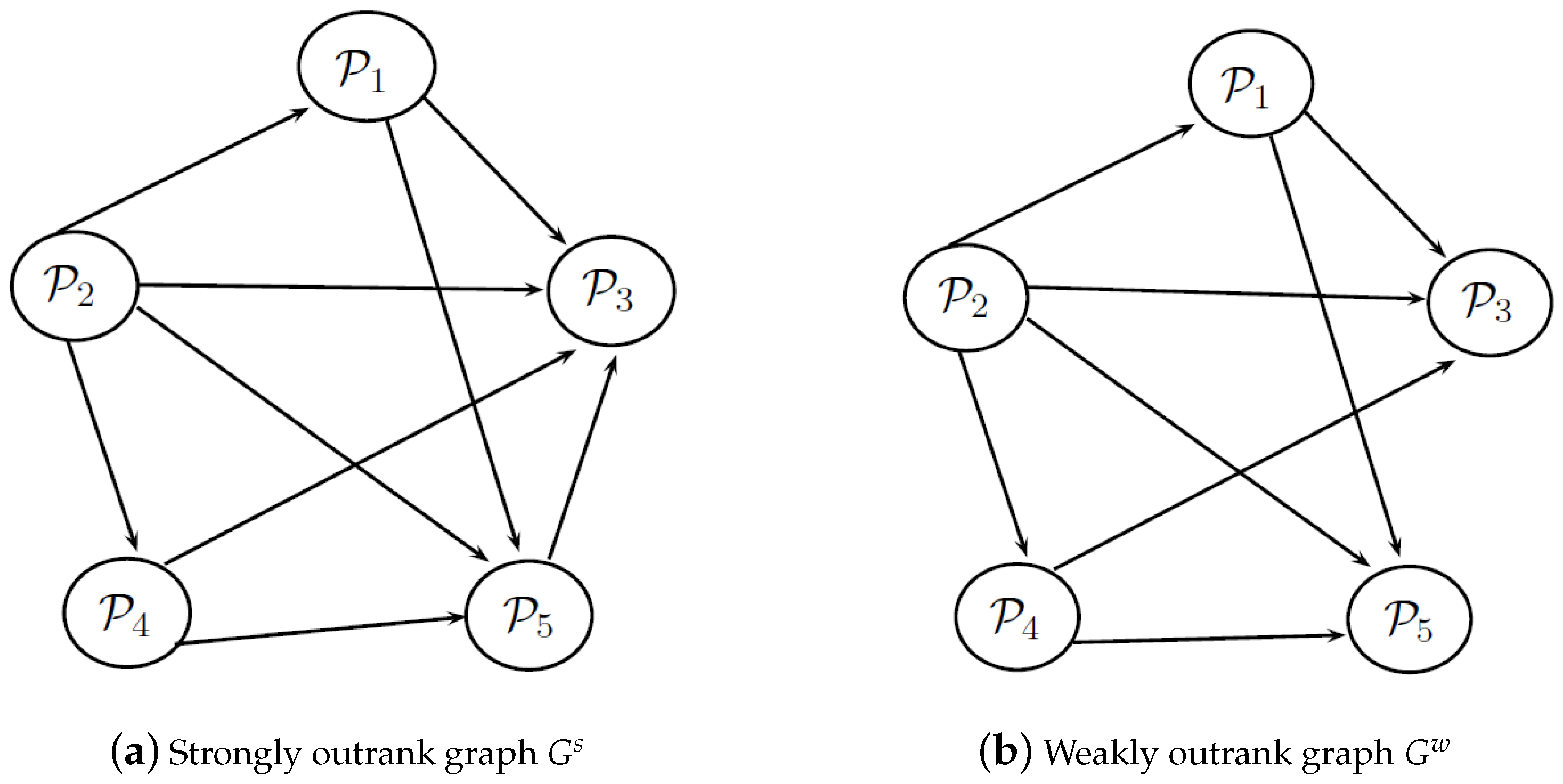
The strongly outrank graph $G^s$ and weakly outrank graph $G^w$ are drawn in Figure 1 according the strong and weak outranking relations, respectively. The outranking graphs are used to find the average ordering of alternatives by following the iterative procedure explained in Section 2.5.

By analyzing these outranking graphs through the iterative procedure mentioned in Section 2.5, the results of forward ranking ${\lambda }^{{}^{\prime }}$, reverse ranking ${\lambda }^{{}^{\prime \prime }}$ and average ranking $\lambda$ are obtained and these rankings are summarized in

Table 4. Ranking results.

	${\mathcal{P}}_1$	${\mathcal{P}}_2$	${\mathcal{P}}_3$	${\mathcal{P}}_4$	${\mathcal{P}}_5$
Forward ranking ${\lambda }^{{}^{\prime }}$	2	1	4	2	3
Reverse ranking ${\lambda }^{{}^{\prime \prime }}$	2	1	5	1	4
Average ranking $\lambda$	2	1	$4.5$	$1.5$	$3.5$

. On the basis of these rankings, the final ranking of the five alternatives is:

$${\mathcal{P}}_2\succ {\mathcal{P}}_4\succ {\mathcal{P}}_1\succ {\mathcal{P}}_5\succ {\mathcal{P}}_3.$$

That is, ${\mathcal{P}}_2$ is best among all other locations.

3.2. Selection of a Supplier

Supplier selection is a procedure by which companies identify, evaluate and contract with suppliers. It is most important to choose a good supplier as many international companies rely on their supply chain network. Selection of an appropriate supplier assure that you are ready to deliver your services or products on time, at the accurate cost and meet your quality standards. Assume that a company is looking for a suitable supplier for its services. After initial screening, a set of five alternatives, $T=\{{\mathcal{P}}_1,{\mathcal{P}}_2,{\mathcal{P}}_3,{\mathcal{P}}_4,{\mathcal{P}}_5\}$, are considered for further evaluation. Further, these alternatives are classified by a set of five criteria $K=\{K_1,K_2,K_3,K_4,K_5\}$ depicting the total cost of opportunity $\left(K_1\right)$, experience in market $\left(K_2\right)$, storage and handling facilities $\left(K_3\right)$, quality and safety $\left(K_4\right)$ and specific methods of delivery $\left(K_5\right)$.

Step 1.

Performance values for each alternative on the basis of conflicting criteria in the form of bipolar fuzzy decision matrix given by a decision maker are presented in

Table 5. Bipolar fuzzy decision matrix.

$\mathcal{L}$	${\mathit{K}}_1$	${\mathit{K}}_2$	${\mathit{K}}_3$	${\mathit{K}}_4$	${\mathit{K}}_5$
${\mathcal{P}}_1$	$(0.8,-0.1)$	$(0.6,-0.3)$	$(0.8,-0.1)$	$(0.8,-0.1)$	$(0.4,-0.7)$
${\mathcal{P}}_2$	$(0.9,-0.1)$	$(0.9,-0.1)$	$(0.8,-0.1)$	$(0.5,-0.5)$	$(0.7,-0.2)$
${\mathcal{P}}_3$	$(0.8,-0.3)$	$(0.6,-0.3)$	$(0.7,-0.1)$	$(0.7,-0.4)$	$(0.8,-0.1)$
${\mathcal{P}}_4$	$(0.9,-0.4)$	$(0.6,-0.2)$	$(0.6,-0.2)$	$(0.8,-0.1)$	$(0.3,-0.7)$
${\mathcal{P}}_5$	$(0.4,-0.6)$	$(0.3,-0.6)$	$(0.8,-0.1)$	$(0.7,-0.3)$	$(0.4,-0.7)$

,

Where each entry ${\ell }_{mn}$ in the matrix represents the positivity and negativity of an alternative ${\mathcal{P}}_m$, $m=1,2,\dots ,5$ for criteria $K_n$, $n=1,2,\dots ,5$. Further, the weights of the criteria are given in vector form as $\omega =[$0.2372 0.2249 0.0685 0.1760 0.2934${]}^T$, which are determined by Equations (1). Clearly, each $0<{\omega }_n<1$ and also satisfy the normalized condition, that is, ${\displaystyle \underset{n=1}{\sum ^s}}{\omega }_n=1$.

Step 2.

The bipolar fuzzy concordance sets $K_{\alpha \beta },K_{{\alpha \beta }^{{}^{\prime }}},K_{{\alpha \beta }^{{}^{\prime \prime }}}$ are enumerated by using Equations (2)–(4), respectively.

(1)

The bipolar fuzzy strong concordance sets $K_{\alpha \beta }$ are given as:

(2)

The bipolar fuzzy median concordance sets $K_{{\alpha \beta }^{{}^{\prime }}}$ are as:

(3)

The bipolar fuzzy weak concordance sets $K_{{\alpha \beta }^{{}^{\prime \prime }}}$ are given as:

The indifferent sets $I_{\alpha \beta }$ are computed by employing Equations (5) as:

The bipolar fuzzy discordance sets $D_{\alpha \beta }$, $D_{{\alpha \beta }^{{}^{\prime }}}$, $D_{{\alpha \beta }^{{}^{\prime \prime }}}$ are established by applying Equations (6)–(8), respectively.

(1)

The bipolar fuzzy strong discordance sets $D_{\alpha \beta }$ are:

(2)

The bipolar fuzzy median discordance sets $D_{{\alpha \beta }^{{}^{\prime }}}$ are:

(3)

The bipolar fuzzy weak discordance sets $D_{{\alpha \beta }^{{}^{\prime \prime }}}$ are:

Step 3.

The importance weights, which are assigned to bipolar fuzzy strong, median, weak concordance sets and indifferent sets by decision maker, are shown in Equations (17). The bipolar fuzzy concordance indices $f_{\alpha \beta },\{\alpha ,\beta =1,2,\cdots ,5,\alpha \ne \beta \}$ are calculated by employing Equations (9), which are used as entries to construct the bipolar fuzzy concordance matrix $F={\left(f_{\alpha \beta }\right)}_{5\times 5}.$

$$\left({\omega }_c,{\omega }_{c^{{}^{\prime }}},{\omega }_{c^{{}^{\prime \prime }}},{\omega }^{=}\right)=\left(1,\frac{3}{4},\frac{2}{4},\frac{1}{4}\right).$$

(17)

For instance, bipolar fuzzy concordance index $f_{12}$ is determined as:

$$\begin{array}{ccc}\hfill f_{12}& =& {\omega }_{c^{{}^{\prime \prime }}}\times \left\{{\omega }_4\right\}+{\omega }^{=}\times \left\{{\omega }_3\right\}\hfill \\ & =& \frac{2}{4}\times 0.1760+\frac{1}{4}\times 0.0685\hfill \\ & =& 0.1015.\hfill \end{array}$$

Step 4.

The weighted distances between any two alternatives with respect to each criteria are calculated by using the bipolar fuzzy Euclidean distance and are shown in

Table 6. Bipolar fuzzy weighted distances.

	${\mathit{\ell }}_{11}$	${\mathit{\ell }}_{21}$	${\mathit{\ell }}_{31}$	${\mathit{\ell }}_{41}$	${\mathit{\ell }}_{51}$		${\mathit{\ell }}_{12}$	${\mathit{\ell }}_{22}$	${\mathit{\ell }}_{32}$	${\mathit{\ell }}_{42}$	${\mathit{\ell }}_{52}$
${\ell }_{11}$	−	$0.0344$	$0.0689$	$0.1089$	$0.2205$	${\ell }_{12}$	−	$0.1209$	0	$0.0335$	$0.1423$
${\ell }_{21}$	−	−	$0.0770$	$0.1033$	$0.2435$	${\ell }_{22}$	−	−	$0.1209$	$0.1060$	$0.2619$
${\ell }_{31}$	−	−	−	$0.0487$	$0.1722$	${\ell }_{32}$	−	−	−	$0.0335$	$0.1423$
${\ell }_{41}$	−	−	−	−	$0.1855$	${\ell }_{42}$	−	−	−	−	$0.1677$
${\ell }_{51}$	−	−	−	−	−	${\ell }_{52}$	−	−	−	−	−
	${\ell }_{\mathbf{13}}$	${\ell }_{\mathbf{23}}$	${\ell }_{\mathbf{33}}$	${\ell }_{\mathbf{43}}$	${\ell }_{\mathbf{53}}$		${\ell }_{\mathbf{14}}$	${\ell }_{\mathbf{24}}$	${\ell }_{\mathbf{34}}$	${\ell }_{\mathbf{44}}$	${\ell }_{\mathbf{54}}$
${\ell }_{13}$	−	0	$0.0185$	$0.0414$	0	${\ell }_{14}$	−	$0.1483$	$0.0938$	0	$0.0663$
${\ell }_{23}$	−	−	$0.0185$	$0.0414$	0	${\ell }_{24}$	−	−	$0.0663$	$0.1483$	$0.0839$
${\ell }_{33}$	−	−	−	$0.0262$	$0.0185$	${\ell }_{34}$	−	−	−	$0.0938$	$0.0297$
${\ell }_{43}$	−	−	−	−	$0.0414$	${\ell }_{44}$	−	−	−	−	$0.0663$
${\ell }_{53}$	−	−	−	−	−	${\ell }_{54}$	−	−	−	−	−
	${\ell }_{\mathbf{15}}$	${\ell }_{\mathbf{25}}$	${\ell }_{\mathbf{35}}$	${\ell }_{\mathbf{45}}$	${\ell }_{\mathbf{55}}$
${\ell }_{15}$	−	$0.2233$	$0.2762$	$0.0383$	0
${\ell }_{25}$	−	−	$0.0542$	$0.2452$	$0.2233$
${\ell }_{35}$	−	−	−	$0.2991$	$0.2761$
${\ell }_{45}$	−	−	−	−	$0.0383$
${\ell }_{55}$	−	−	−	−	−

.

For example, the Euclidean distance between ${\ell }_{11}$ and ${\ell }_{21}$ with respect to criteria $K_1$ is calculated as

$$\begin{array}{ccc}\hfill d({\omega }_1{\ell }_{11},{\omega }_1{\ell }_{21})& =& \sqrt{\frac{1}{2}\times {\omega }_1[{({\mu }_{11}-{\mu }_{21})}^2+{({\nu }_{11}-{\nu }_{21})}^2]}\hfill \\ & =& \sqrt{\frac{1}{2}\times 0.2372[{(0.8-0.9)}^2+{(-0.1-(-0.1))}^2]}\hfill \\ & =& 0.0344.\hfill \end{array}$$

Similarly, $d({\omega }_2{\ell }_{12},{\omega }_2{\ell }_{22})=0.1209$, $d({\omega }_3{\ell }_{13},{\omega }_3{\ell }_{23})=0$, $d({\omega }_4{\ell }_{14},{\omega }_4{\ell }_{24})=0.1483$, $d({\omega }_5{b}_{15},{\omega }_5{b}_{25})=0.2233$ and others.

Step 5.

The importance weights, which are assigned to bipolar fuzzy strong, median and weak discordance sets by decision maker, are shown in Equations (18). The bipolar fuzzy discordance indices $t_{\alpha \beta },\{\alpha ,\beta =1,2,\cdots ,5,\alpha \ne \beta \}$ are calculated by applying Equations (10), which are used as entries to construct the bipolar fuzzy discordance matrix $H={\left(t_{\alpha \beta }\right)}_{5\times 5}.$

$$\left({\omega }_d,{\omega }_{d^{{}^{\prime }}},{\omega }_{d^{{}^{\prime \prime }}}\right)=\left(1,\frac{3}{4},\frac{2}{4}\right).$$

(18)

For instance, the bipolar fuzzy discordance index $t_{12}$ is determined as:

$$\begin{array}{ccc}\hfill t_{12}& =& \frac{max\left\{{\omega }_{d^{{}^{\prime }}}\times d({\omega }_1{\ell }_{11},{\omega }_1{\ell }_{21}),{\omega }_{d^{{}^{\prime \prime }}}\times d({\omega }_2{\ell }_{12},{\omega }_1{\ell }_{22}),{\omega }_{d^{{}^{\prime \prime }}}\times d({\omega }_5{\ell }_{15},{\omega }_4{\ell }_{25})\right\}}{\underset{n\in J}{max}d({\omega }_n{\ell }_{\alpha n},{\omega }_n{\ell }_{\beta n})}\hfill \\ & =& \frac{max\left\{\frac{3}{4}\times 0.0344,\frac{2}{4}\times 0.1209,\frac{2}{4}\times 0.2233\right\}}{max\left\{0.0344,0.1209,0,0.1483,0.2233\right\}}\hfill \\ & =& \frac{max\{0.0258,0.0605,0.1117\}}{max\{0.0344,0.1209,0,0.1483,0.2233\}}\hfill \\ & =& \frac{0.1117}{0.2233}=0.5002.\hfill \end{array}$$

Step 6.

The outranking relationships between the alternatives, as strong outranking relation $R^s$ and weak outranking relation $R^w$, are computed by comparing the entries of bipolar fuzzy concordance and discordance matrices along with the concordance and discordance levels which are specified by decision maker as:

$$(f^{*},f^{\circ },f^{-})=(0.4,0.3,0.2),(t^{*},t^{\circ })=(0.3,0.5).$$

The strong and weak outranking relations are established by applying Equations (11) and (12), respectively, and are shown in

Table 7. Outranking relation.

	${\mathcal{P}}_1$	${\mathcal{P}}_2$	${\mathcal{P}}_3$	${\mathcal{P}}_4$	${\mathcal{P}}_5$
${\mathcal{P}}_1$	−	0	0	0	$R^s,R^w$
${\mathcal{P}}_2$	$R^s$	−	$R^w$	$R^s$	$R^s,R^w$
${\mathcal{P}}_3$	$R^s,R^w$	0	−	0	$R^s,R^w$
${\mathcal{P}}_4$	0	0	0	−	$R^s,R^w$
${\mathcal{P}}_5$	0	0	0	0	−

.

Step 7.

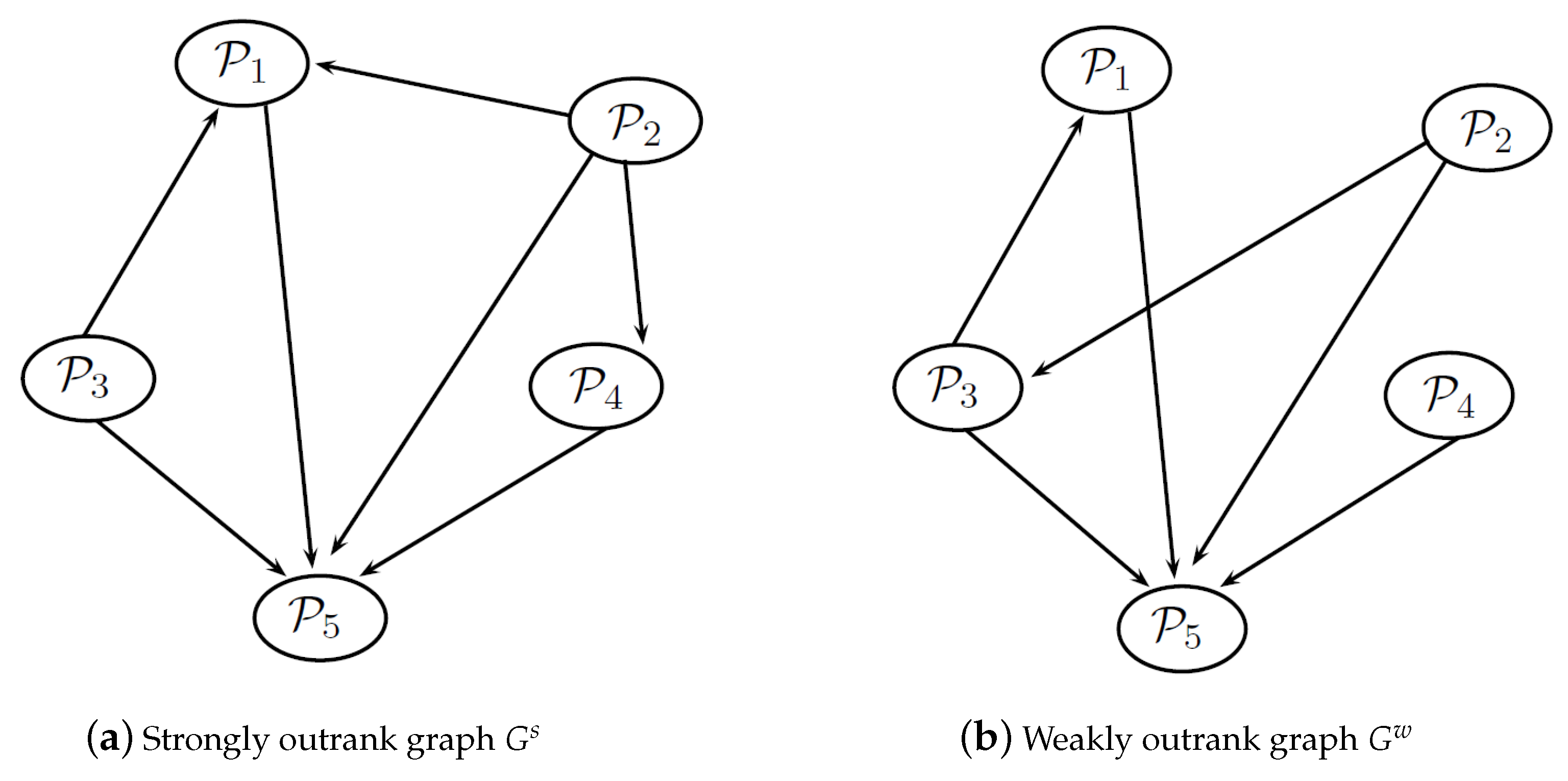
The strongly outrank graph $G^s$ and weakly outrank graph $G^w$ are drawn in Figure 2 according the strong and weak outranking relations, respectively. These outranking graphs are used to find the average ordering of alternatives by following the iterative procedure explained in Section 2.5.

By analyzing these outranking graphs through the iterative procedure mentioned in Section 2.5, the results of forward ranking ${\lambda }^{{}^{\prime }}$, reverse ranking ${\lambda }^{{}^{\prime \prime }}$ and the average ranking $\lambda$ are obtained and these rankings are summarized in

Table 8. Ranking results.

	${\mathcal{P}}_1$	${\mathcal{P}}_2$	${\mathcal{P}}_3$	${\mathcal{P}}_4$	${\mathcal{P}}_5$
Forward ranking ${\lambda }^{{}^{\prime }}$	3	1	2	2	4
Reverse ranking ${\lambda }^{{}^{\prime \prime }}$	3	1	2	3	4
Average ranking $\lambda$	3	1	2	$2.5$	4

. Finally, on the basis of average ranking, these five alternative are ranked as:

$${\mathcal{P}}_2\succ {\mathcal{P}}_3\succ {\mathcal{P}}_4\succ {\mathcal{P}}_1\succ {\mathcal{P}}_5.$$

4. Discussion and Comparative Study

This section provides a comparative analysis of presented bipolar fuzzy ELECTRE II method with already existing MADM methods such as TOPSIS and ELECTRE I models under bipolar fuzzy environment, which were presented by Alghamdi et al. [29]. We applied these methods to the numerical problem presented in Section 3.1, as “selection of business location” to compare the different MCDM methods. A discussion and theoretical comparison of BF-ELECTRE II method is also presented with fuzzy ELECTRE II method, which was proposed by Govindan et al. [20].

4.1. Bipolar Fuzzy TOPSIS Method

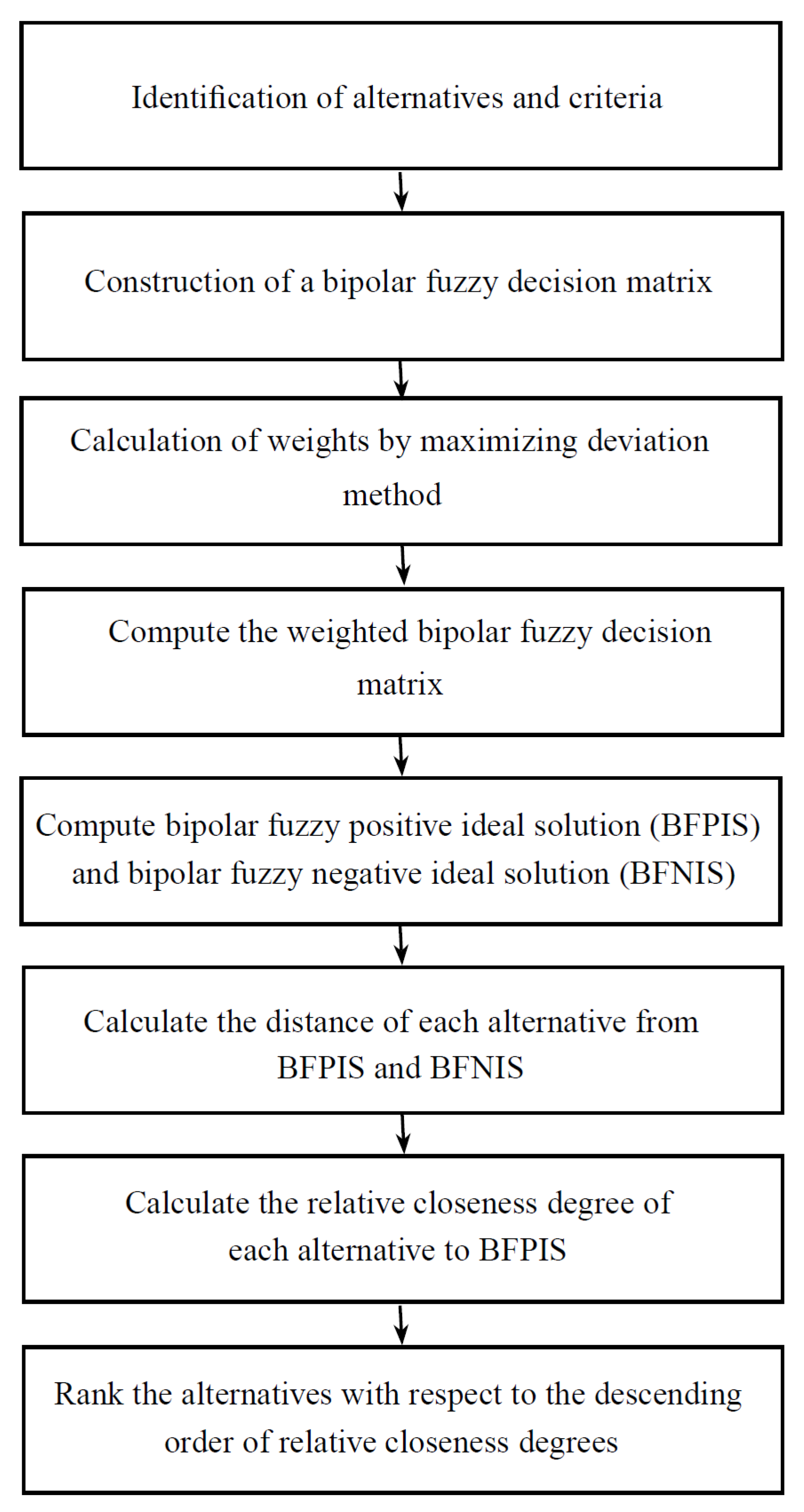
A flow chart of general steps of bipolar fuzzy TOPSIS method, presented by Alghamdi et al. [29], is given in Figure 3. In this subsection, the problem to select the business location is solved by using bipolar fuzzy TOPSIS method. The steps for the construction of bipolar fuzzy decision matrix and the calculation of weights are the same as described in bipolar fuzzy ELECTRE II method. Consider the bipolar fuzzy decision matrix given in Table 1, and construct a weighted bipolar fuzzy decision matrix by multiplying the weight vector to decision matrix, which is given in

Table 9. Weighted bipolar fuzzy decision matrix.

	${\mathit{K}}_1$	${\mathit{K}}_2$	${\mathit{K}}_3$	${\mathit{K}}_4$	${\mathit{K}}_5$
${\mathcal{P}}_1$	$(0.0687,-0.1375)$	$(0.2001,-0.0734)$	$(0.0990,-0.1187)$	$(0.0712,-0.1192)$	$(0.1307,-0.0762)$
${\mathcal{P}}_2$	$(0.1178,-0.0491)$	$(0.0889,-0.1556)$	$(0.1286,-0.1583)$	$(0.1490,-0.0083)$	$(0.2178,-0.0545)$
${\mathcal{P}}_3$	$(0.0393,-0.0982)$	$(0.0622,-0.1334)$	$(0.0732,-0.1187)$	$(0.0546,-0.0994)$	$(0.1742,-0.0871)$
${\mathcal{P}}_4$	$(0.0923,-0.1277)$	$(0.1223,-0.0600)$	$(0.0495,-0.0990)$	$(0.0911,-0.0662)$	$(0.1634,-0.1307)$
${\mathcal{P}}_5$	$(0.1571,-0.0589)$	$(0.0667,-0.0333)$	$(0.1979,-0.0792)$	$(0.1159,-0.0530)$	$(0.0653,-0.1742)$

.

The bipolar fuzzy positive ideal solution (BFPIS) and bipolar fuzzy negative ideal solution (BFNIS) for each criteria are computed as follows:

$$\begin{array}{cc}\hfill BFPIS& =\left[\right(0.1571,-0.0491),(0.2001,-0.0333),(0.1979,-0.0792),(0.1490,-0.0530),(0.2178,-0.0545\left)\right],\hfill \\ \hfill BFNIS& =\left[\right(0.0393,-0.1375),(0.0622,-0.1556),(0.0495,-0.1583),(0.0546,-0.1192),(0.0653,-0.1742\left)\right].\hfill \end{array}$$

Furthermore, the Euclidean distance of each alternative from BFPIS and BFNIS is enumerated as:

$$\begin{array}{cc}\hfill D({\mathcal{P}}_1,BFPIS)& =0.153,D({\mathcal{P}}_1,BFNIS)=0.150,\hfill \\ \hfill D({\mathcal{P}}_2,BFPIS)& =0.143,D({\mathcal{P}}_2,BFNIS)=0.185,\hfill \\ \hfill D({\mathcal{P}}_3,BFPIS)& =0.196,D({\mathcal{P}}_3,BFNIS)=0.110,\hfill \\ \hfill D({\mathcal{P}}_4,BFPIS)& =0.161,D({\mathcal{P}}_4,BFNIS)=0.132,\hfill \\ \hfill D({\mathcal{P}}_5,BFPIS)& =0.168,D({\mathcal{P}}_5,BFNIS)=0.189.\hfill \end{array}$$

The relative closeness degree of each alternative to BFPIS is calculated as follows:

$$C\left({\mathcal{P}}_1\right)=0.495,C\left({\mathcal{P}}_2\right)=0.564,C\left({\mathcal{P}}_3\right)=0.359,C\left({\mathcal{P}}_4\right)=0.451,C\left({\mathcal{P}}_5\right)=0.529.$$

According to these closeness coefficients, the alternatives are ranked in descending order as ${\mathcal{P}}_2\succ {\mathcal{P}}_5\succ {\mathcal{P}}_1\succ {\mathcal{P}}_4\succ {\mathcal{P}}_3$, and thus location ${\mathcal{P}}_2$ is the best choice with maximum closeness degree.

4.2. Bipolar Fuzzy ELECTRE I Method

A flow chart of the general steps of bipolar fuzzy ELECTRE I method is given in Figure 4.

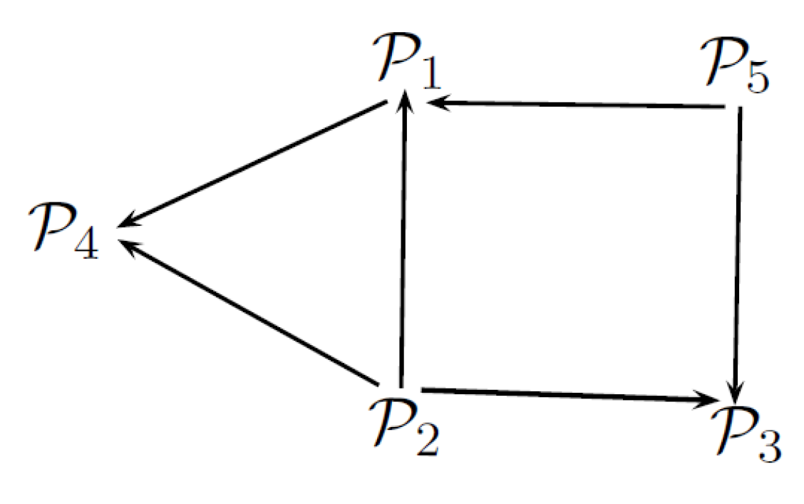
To solve the same problem of business location by employing the bipolar fuzzy ELECTRE I method, consider the weighted bipolar fuzzy decision matrix given in Table 9, and follow the next steps of bipolar fuzzy ELECTRE I method to determine an outranking relation of alternatives in order to compare these multi-attribute decision making methods. The evaluation of bipolar fuzzy concordance sets ${\mathbb{C}}_{\alpha \beta }$, bipolar fuzzy discordance sets ${\mathbb{D}}_{\alpha \beta }$, bipolar fuzzy concordance indices $c_{\alpha \beta }$, bipolar fuzzy discordance indices $d_{\alpha \beta }$, concordance dominance $g_{\alpha \beta }$, discordance dominance $h_{\alpha \beta }$, aggregated dominance $q_{\alpha \beta }$ and outranking relations for this problem is briefly summarized in

Table 10. Bipolar Fuzzy ELECTRE I results for selection of Business location.

Alternatives Compared	${\mathbb{C}}_{\mathit{\alpha }\mathit{\beta }}$	${\mathbb{D}}_{\mathit{\alpha }\mathit{\beta }}$	${\mathit{c}}_{\mathit{\alpha }\mathit{\beta }}$	${\mathit{d}}_{\mathit{\alpha }\mathit{\beta }}$	${\mathit{g}}_{\mathit{\alpha }\mathit{\beta }}$	${\mathit{h}}_{\mathit{\alpha }\mathit{\beta }}$	${\mathit{q}}_{\mathit{\alpha }\mathit{\beta }}$	Outranking Relations
$({\mathcal{P}}_1,{\mathcal{P}}_2)$	$\{2,3\}$	$\{1,4,5\}$	$0.4202$	1	0	0	0	Incomparable
$({\mathcal{P}}_1,{\mathcal{P}}_3)$	$\{2,3\}$	$\{1,4,5\}$	$0.4202$	$0.5893$	0	1	0	Incomparable
$({\mathcal{P}}_1,{\mathcal{P}}_4)$	$\{2,3,5\}$	$\{1,4\}$	$0.6380$	$0.5187$	1	1	1	${\mathcal{P}}_1\to {\mathcal{P}}_4$
$({\mathcal{P}}_1,{\mathcal{P}}_5)$	$\{2,5\}$	$\{1,3,4\}$	$0.4401$	1	0	0	0	Incomparable
$({\mathcal{P}}_2,{\mathcal{P}}_1)$	$\{1,4,5\}$	$\{2,3\}$	$0.5798$	$0.5514$	1	1	1	${\mathcal{P}}_2\to {\mathcal{P}}_1$
$({\mathcal{P}}_2,{\mathcal{P}}_3)$	$\{1,2,3,4,5\}$	$\left\{\right\}$	1	0	1	1	1	${\mathcal{P}}_2\to {\mathcal{P}}_3$
$({\mathcal{P}}_2,{\mathcal{P}}_4)$	$\{1,3,4,5\}$	$\left\{2\right\}$	$0.7777$	$0.0336$	1	1	1	${\mathcal{P}}_2\to {\mathcal{P}}_4$
$({\mathcal{P}}_2,{\mathcal{P}}_5)$	{4,5}	$\{1,2,3\}$	$0.3834$	1	0	0	0	Incomparable
$({\mathcal{P}}_3,{\mathcal{P}}_1$)	$\{1,4,5\}$	$\{2,3\}$	$0.5798$	1	1	0	0	Incomparable
$({\mathcal{P}}_3,{\mathcal{P}}_2)$	$\left\{\right\}$	$\{1,2,3,4,5\}$	0	1	0	0	0	Incomparable
$({\mathcal{P}}_3,{\mathcal{P}}_4)$	$\{3,5\}$	$\{1,2,4\}$	$0.4157$	$0.4312$	0	1	0	Incomparable
$({\mathcal{P}}_3,{\mathcal{P}}_5)$	$\left\{5\right\}$	$\{1,2,3,4\}$	$0.2178$	1	0	0	0	Incomparable
$({\mathcal{P}}_4,{\mathcal{P}}_1)$	$\{1,4\}$	$\{2,3,5\}$	$0.3620$	1	0	0	0	Incomparable
$({\mathcal{P}}_4,{\mathcal{P}}_2)$	$\left\{2\right\}$	$\{1,3,4,5\}$	$0.2223$	1	0	0	0	Incomparable
$({\mathcal{P}}_4,{\mathcal{P}}_3)$	$\{1,2,4\}$	$\{3,5\}$	$0.5843$	1	1	0	0	Incomparable
$({\mathcal{P}}_4,{\mathcal{P}}_5)$	$\{2,5\}$	$\{1,3,4\}$	$0.4401$	$0.8237$	0	0	0	Incomparable
$({\mathcal{P}}_5,{\mathcal{P}}_1)$	$\{1,3,4\}$	$\{2,5\}$	$0.5599$	$0.1332$	1	1	1	${\mathcal{P}}_5\to {\mathcal{P}}_1$
$({\mathcal{P}}_5,{\mathcal{P}}_2)$	$\{1,2,3,\}$	$\{4,5\}$	$0.6166$	$0.8744$	1	0	0	Incomparable
$({\mathcal{P}}_5,{\mathcal{P}}_3)$	$\{1,2,3,4\}$	$\left\{5\right\}$	$0.7822$	$0.2973$	1	1	1	${\mathcal{P}}_5\to {\mathcal{P}}_3$
$({\mathcal{P}}_5,{\mathcal{P}}_4)$	$\{1,3,4\}$	$\{2,5\}$	$0.5599$	1	1	0	0	Incomparable

. The graph sketch by outranking relations is given in Figure 5 and the set of most favorable alternatives is $\{{\mathcal{P}}_2,{\mathcal{P}}_5\}$.

It is clearly shown that the alternative ${\mathcal{P}}_2$ is chosen as the best possible location for all these MCDM methods under bipolar fuzzy environment. Thus, the proposed bipolar fuzzy ELECTRE II method can be successfully applied to solve the MCDM problems with bipolar fuzzy information. This method not only gives the solution of problem but also ranks the alternatives in ascending order and the alternative with minimum choice value is chosen as best action.

4.3. Comparison of BF-ELECTRE II with Fuzzy ELECTRE II

• Bipolar fuzzy set plays an important role in human decision making, as it deals with two-sided information or bipolar reasoning of human thinking. Positive information represents what is granted to be possible or true, while negative information represents what is considered to be impossible or may be false. There are many real world problems which are based on bipolarity or double-sided information (instead of one-sided), as we described in the numerical examples. We use bipolar fuzzy set in which the performance rating of each alternative consists of two membership values: positive and negative. The positive membership value of an alternative shows the benefit or satisfaction behavior of that alternative towards the criteria and the negative membership value represents the cost or dissatisfaction degree of alternatives. We use bipolar fuzzy ELECTRE II method to rank the alternatives in ascending order or to chose the best possible action.
• Fuzzy ELECTRE II is successfully applied to solve problems having only one sided information, that is, alternatives are ranked only on the basis of positive membership or satisfaction degree of alternatives. By using fuzzy structure or set to decision making, we are unable to provide information about the dissatisfaction behavior or degree of alternatives corresponding to different criteria. Thus, we present BF-ELECTRE II method to rank the alternatives as an improvement of other successful versions of ELECTRE II method.

5. Insights and Limitations of Proposed Method

Some insights of proposed BF-ELECTRE II method are:

• The presented BF-ELECTRE II method is an extension of other existing versions of ELECTRE II method to rank alternatives, as it deals with bipolar fuzzy information.
• An optimization technique based on maximizing deviation method is used to calculate the normalized weights of criteria to minimize the personal interest of decision makers towards the criteria.
• Two types of outranking relations are used to obtain more appropriate results and an iterative procedure is followed to rank the alternatives.
• Two numerical examples are explained by using this method.

Beside of all above discussion, this method also has some limitations:

• This method is appropriate for dealing with two-sided information of human thinking, but it cannot appropriately handle the m-sided or m-polar information.
• Another limitation of this method is its great dependance on decision maker’s choice for computing the important weights and threshold values.

6. Conclusions

Multiple-attribute decision making (MADM) provides valuable tools to deal with complex problems and make effective and convenient decisions. In this research article, we present a multiple-criteria decision making method named bipolar fuzzy ELECTRE II, which is proposed by joining the ELECTRE II method with bipolar fuzzy information to solve problems having bipolar uncertainties. The implementation and flexibility of the proposed method are explained through a step-by-step procedure. It was validated by real world problems, in which alternatives were ranked by following its methodology. The outranking relations, such as strong outranking relation and weak outranking relation, are established on the basis of bipolar fuzzy strong, median and weak concordance as well as discordance sets and indifferent set. An optimization technique based on maximizing deviation method is applied to compute the normalized weights of conflicting criteria. An iterative procedure is applied to rank the alternatives and find the best possible solution. We compared bipolar fuzzy ELECTRE II method with already existing MADM methods, such as bipolar fuzzy TOPSIS and bipolar fuzzy ELECTRE I, by solving the same problem of selecting a business location. The obtained results indicate that this method can be successfully adopted for multi-criteria decision making problems, not only giving an appropriate choice of action but also ranking the alternatives in ascending order. We aim to broaden our study to: (1) complex fuzzy ELECTRE II method; (2) complex bipolar neutrosophic ELECTRE III method; and (3) bipolar fuzzy ELECTRE III method.

References

- Saaty, T.L. Axiomatic foundation of the analytic hierarchy process. Manag. Sci. 1986, 32, 841–855. [Google Scholar] [CrossRef]
- Hwang, C.L.; Yoon, K. Multiple Attribute Decision Making Methods and Applications; Springer: Berlin, Germany, 1981. [Google Scholar]
- Opricovic, S.; Tzeng, G.H. Compromise solution by MCDM methods: A comparative analysis of VIKOR and TOPSIS. Eur. J. Oper. Res. 2004, 156, 445–455. [Google Scholar] [CrossRef]
- Benayoun, R.; Roy, B.; Sussman, B. Electre: Une methode pour guider le choix en presence de points de vue multiples; Technical Report; SEMA-METRA International, Direction Scientifique: Paris, France, 1966. [Google Scholar]
- Brans, J.P.; Vincke, P.; Mareschal, B. How to select and how to rank projects: The PROMETHEE method. Eur. J. Oper. Res. 1986, 24, 228–238. [Google Scholar] [CrossRef]
- Bellman, R.E.; Zadeh, L.A. Decision-making in a fuzzy environment. Manag. Sci. 1970, 4, 141–164. [Google Scholar] [CrossRef]
- Roy, B. The Outranking Approach and The Foundations of Electre Methods, in Readings in Multiple Criteria Decision Aid; Springer: Berlin/Heidelberg, Germany, 1990; pp. 155–183. [Google Scholar]
- Hatami-Marbini, A.; Tavana, M. An extension of the ELECTRE method for group decision making under a fuzzy environment. Omega 2011, 39, 373–386. [Google Scholar] [CrossRef]
- Akram, M.; Ilyas, F.; Garg, H. Multi-criteria group decision making based on ELECTRE I method in Pythagorean fuzzy information. Soft Comput. 2019, 1–29. [Google Scholar] [CrossRef]
- Akram, M.; Shumaiza; Smarandache, F. Decision-making with bipolar neutrosophic TOPSIS and bipolar neutrosophic ELECTRE-I. Axioms 2018, 7, 33. [Google Scholar] [CrossRef]
- de Almeida, A.T. Multicriteria decision model for outsourcing contracts selection based on utility function and ELECTRE method. Comput. Oper. Res. 2007, 34, 3569–3574. [Google Scholar] [CrossRef]
- Aiello, G.; Enea, M.; Galante, G. A multi-objective approach to facility layout problem by genetic search algorithm and Electre method. Robot.-Comput.-Integr. Manuf. 2006, 22, 447–455. [Google Scholar] [CrossRef]
- Beccali, M.; Cellura, M.; Mistretta, M. Decision-making in energy planning, Application of the Electre method at regional level for the diffusion of renewable energy technology. Renew. Energy 2003, 28, 2063–2087. [Google Scholar] [CrossRef]
- Wen, Z.; Yu, Y.; Yan, J. Best available techniques assessment for coal gasification to promote cleaner production based on the ELECTRE-II method. J. Clean. Prod. 2016, 129, 12–22. [Google Scholar] [CrossRef]
- Buchanan, J.; Vanderpooten, D. Ranking projects for an electricity utility using ELECTRE III. Int. Trans. Oper. Res. 2007, 14, 309–323. [Google Scholar] [CrossRef]
- Chen, T.Y. An ELECTRE-based outranking method for multiple criteria group decision making using interval type-2 fuzzy sets. Inf. Sci. 2014, 263, 1–21. [Google Scholar] [CrossRef]
- Vahdani, B.; Hadipour, H. Extension of the ELECTRE method based on interval-valued fuzzy sets. Soft Comput. 2011, 15, 569–579. [Google Scholar] [CrossRef]
- Roy, B.; La, P. Methode Electre II. Note de travail 1971, 142. [Google Scholar]
- Zadeh, L.A. Fuzzy sets. Inf. Control. 1965, 8, 338–353. [Google Scholar] [CrossRef] [Green Version]
- Govindan, K.; Grigore, M.C.; Kannan, D. Ranking of third party logistics provider using fuzzy Electre II. In Proceedings of the 40th International Conference on Computers and Indutr Bertier ial Engineering, Awaji Island, Japan, 25–28 July 2010; pp. 1–5. [Google Scholar]
- Devadoss, A.V.; Rekha, M. A New Intuitionistic Fuzzy ELECTRE II approach to study the Inequality of women in the society. Glob. J. Pure Appl. Math. 2017, 13, 6583–6594. [Google Scholar]
- Duckstein, L.; Gershon, M. Multicriterion analysis of a vegetation management problem using ELECTRE II. Appl. Math. Model. 1983, 7, 254–261. [Google Scholar] [CrossRef]
- Chen, N.; Xu, Z. Hesitant fuzzy ELECTRE II approach: a new way to handle multi-criteria decision making problems. Inf. Sci. 2015, 292, 175–197. [Google Scholar] [CrossRef]
- Huang, W.C.; Chen, C.H. Using the ELECTRE II method to apply and analyze the differentiation theory. Proc. East. Asia Soc. Transp. Stud. 2005, 5, 2237–2249. [Google Scholar]
- Wang, L.; Liao, B.; Liu, X.; Liu, J. Possibility-based ELECTRE II method with uncertain linguistic fuzzy variables. Int. J. Pattern Recognit. Artif. Intell. 2017, 31, 1759016. [Google Scholar] [CrossRef]
- Liao, H.C.; Yang, L.Y.; Xu, Z.S. Two new approaches based on ELECTRE II to solve the multiple criteria decision making problems with hesitant fuzzy linguistic term sets. Appl. Soft Comput. 2018, 63, 223–234. [Google Scholar] [CrossRef]
- Zhang, W.R. Bipolar fuzzy sets and relations: a computational framework for cognitive modeling and multiagent decision analysis. In Proceedings of the IEEE Conference Fuzzy Information Processing Society Biannual Conference, San Antonio, TX, USA, 18–21 December 1994; pp. 305–309. [Google Scholar]
- Zhang, W.R. YingYang Bipolar fuzzy sets. IEEE Int. Conf. Fuzzy Syst. 1998, 1, 835–840. [Google Scholar]
- Alghamdi, M.A.; Alshehri, N.O.; Akram, M. Multi-criteria decision-making methods in bipolar fuzzy environment. Int. J. Fuzzy Syst. 2018, 20, 2057–2064. [Google Scholar] [CrossRef]
- Akram, M.; Arshad, M. A novel trapezoidal bipolar fuzzy TOPSIS method for group decision-making. Group Decis. Negot. 2019, 28, 565–584. [Google Scholar] [CrossRef]
- Akram, M.; Shumaiza; Arshad, M. Bipolar fuzzy TOPSIS and bipolar fuzzy ELECTRE-I methods to diagnosis. Comput. Appl. Math. 2019. [Google Scholar] [CrossRef]
- Shumaiza; Akram, M.; Al-Kenani, A.N.; Alcantud, J.C.R. Group decision-making based on the VIKOR method with trapezoidal bipolar fuzzy information. Symmetry 2019, 11, 1313. [Google Scholar] [CrossRef]
- Akram, M.; Dudek, W.A.; Ilyas, F. Group decision-making based on pythagorean fuzzy TOPSIS method. Int. J. Intell. Syst. 2019, 34, 1455–1475. [Google Scholar] [CrossRef]
Figure 1.
Graphical representation of outranking relations between alternatives.
Figure 2.
Figure 3.
The steps of bipolar fuzzy TOPSIS model.
Figure 4.
The steps of bipolar fuzzy ELECTRE I method.
Figure 5.
Graph representing the outranking relation of alternatives.