Modeling and Solving Scheduling Problem with m Uniform Parallel Machines Subject to Unavailability Constraints

Abstract

The problem investigated in this paper is scheduling on uniform parallel machines, taking into account that machines can be periodically unavailable during the planning horizon. The objective is to determine planning for job processing so that the makespan is minimal. The problem is known to be NP-hard. A new quadratic model was developed. Because of the limitation of the aforementioned model in terms of problem sizes, a novel algorithm was developed to tackle big-sized instances. This consists of mainly two phases. The first phase generates schedules using a modified Largest Processing Time ($LPT$)-based procedure. Then, theses schedules are subject to further improvement during the second phase. This improvement is obtained by simultaneously applying pairwise job interchanges between machines. The proposed algorithm and the quadratic model were implemented and tested on variously sized problems. Computational results showed that the developed quadratic model could optimally solve small- to medium-sized problem instances. However, the proposed algorithm was able to optimally solve large-sized problems in a reasonable time.

1. Introduction

In the industry field, machines are often supposed to be continuously available for processing assigned jobs. However, this assumption is not totally realistic in real-world cases. For instance, machines may be subject to unavailability periods due to many reasons, such as preventive maintenance [1], corrective maintenance [2], and tool-change activities [3]. There are two main concerns related to the temporary unavailability of a machine. The first is related to the increased costs caused by stopping the machine’s activity, while the second is linked to the difficulty in taking decisions regarding the balance between resource unavailability and production. Therefore, a proper planning strategy in a manufacturing system is necessary for it to operate in the most cost-effective way.

Scheduling under machine-unavailability constraints has attracted the attention of many researchers, and many real applications can be found. In [4], the authors listed two applications in the aerospace industry where the machine must be stopped to change microdrilling tools after a fixed number of use times. Another application was mentioned by [5] related to electric-battery vehicles that require refuelling operations.

In this paper, we study a scheduling problem on m uniform parallel machines with multiple unavailability constraints with the objective to minimize the makespan, which is the completion time of the last assigned job. The reason behind the choice of such an objective is that minimizing the makespan can ensure a good load balance among the machines. We followed three-field $\alpha \left|\beta \right|\gamma$ classification, developed by [6], to represent the problem as $Qm,h_{ik}\left|a\right|\gamma$. In the first field, Q denotes uniform parallel machine setting, m represents the number of considered machines, and $h_{ik}$ states that each machine is unavailable during k periods in the planning horizon. In the second field, $\beta$, a indicates that the machines are subject to availability constraints. Lastly, the third field, $\gamma$, describes the objective to be minimized, that is, the completion time of the last processed job, denoted by $C_{max}$.

Many papers in the literature studied parallel machine-scheduling problems with availability constraints, but very few considered a uniform parallel machine setting. To the best of our knowledge, only two related papers exist so far, [7,8]. In [7], the authors studied the uniform parallel machine-scheduling problem where each machine could be unavailable during one period of time. The considered performance measures were total completion times and makespan. Two types of jobs were treated, namely, identical and nonidentical jobs. Linear programming models and optimal algorithms were developed to solve the problem where jobs are identical. For the case of nonidentical jobs, the authors proved that the problem is NP-hard, and proposed a quadratic program and a heuristic that were tested on large-sized problem instances. The online version of the problem was studied in [8]. The authors considered the case of two machines under the constraint of one periodically unavailable machine. The identical- and uniform-machine cases were investigated. The objective was to minimize the makespan. The solution approach consisted of optimal algorithms with competitive ratios.

Furthermore, most research papers studied the case of identical parallel machines. For example, [9,10,11,12,13] studied various identical parallel machine problems allowing various types of unavailable intervals for machines.

The shortage in research in this area, and the important applications of the investigated problem in reality motivated the author of this paper to explore this area more and contribute to the scientific research on it. Uniform parallel machine scheduling can be found in the manufacturing field where the same type of job can be processed on new and old machines that have different speeds. As an example, a printing task can take much more time on an old machine than on a new one.

In this paper, the main contributions are a quadratic programming-model (QM) formulation of a uniform parallel machine with multiple availability constraints and an algorithm that provides optimal solutions. To the best of our knowledge, the proposed QM is the first such formulation for scheduling on uniform parallel machine with availability constraints.

The content of this paper is organized as follows. Problem notations are laid in Section 2. In Section 3.1, a quadratic model for the problem with makespan as an objective is developed. Section 3.2 details an algorithm proposed for makespan-performance measurement. The proposed algorithm was tested on different problem instances, and results are displayed in Section 4. Finally, a general conclusion is formulated in Section 5.

2. Notations

For accuracy of description, by ‘unavailability interval’ we denote the time interval in which the machine is not available for processing any job, whereas the time interval between two consecutive unavailability intervals is called the ‘availability interval’ of the machine.

In this paper, we consider m uniform parallel machines that can process n jobs. Each job j, $j=1,\dots ,n$ is characterized by processing time $p_j$ and completion time $C_j$. We assumed that the jobs were ready at time 0 and could be processed once at any time, but could not be interrupted once started. Since we consider uniform parallel machines, each machine i, $i=1,\dots ,m$, can process at most one job at a time at speed $s_i$. So, the processing time of any job j depends on the machine on which it is processed and is equal to $p_{ij}=p_j/s_i$, $i=1,\dots ,m$; $j=1,\dots ,n$. Without loss of generality, we assumed that jobs were indexed in $LPT$ order, that is, $p_{i1}\ge p_{i2}\ge \dots \ge p_{in}$. We assumed that the machine could process the next job once the previous one was finished. Thus, no setup time was considered. Let $s_{ik}$ and $e_{ik}$ be the starting and ending time of the $k^{th}$ unavailability period on machine i, respectively. Without loss of generality, we assumed that all machines were available at the beginning of the planning horizon. By $L_{ik}$, we denote the length of the $k^{th}$ availability interval on machine i.

The problem was to find a job assignment on machines that minimizes the makespan. As stated earlier, the problem of scheduling jobs on uniform parallel machines subject to unavailability constraints has not been studied before. Therefore, a mathematical formulation of the problem can be of great interest. Thus, in Section 3.1, we detail a mathematical model to describe the problem under consideration.

3. Proposed Solution Approach for $Qm,h_{i{n}_i}\left|a\right|C_{max}$

In this section, we studied the scheduling problem on uniform parallel machine, where each machine i can be unavailable during $n_i$ unavailability periods in its planning horizon. Thus, there are $n_i+1$ availability intervals. The objective was to minimize the makespan.

It is easy to see that $Qm,h_{i{n}_i}\left|a\right|C_{max}$ is NP-hard. To see this, let $s_i=1$ for every machine $i.$ Then the problem reduces to the identical parallel machine-scheduling problem under availability constraints that was proved to be NP-hard by [14].

3.1. Mathematical Model

Let

$$x_{ijk}=\left\{\begin{array}{cc}\hfill 1& \mathrm{if}\mathrm{job}j\mathrm{is}\mathrm{executed}\mathrm{on}\mathrm{machine}i\mathrm{during}{k}^{th}\mathrm{availability}\mathrm{interval}\hfill \\ \hfill 0& \mathrm{Otherwise}.\hfill \end{array}\right.$$

$$y_{ik}=\left\{\begin{array}{cc}\hfill 1& \mathrm{if}\mathrm{all}\mathrm{jobs}\mathrm{on}\mathrm{machine}i\mathrm{are}\mathrm{completed}\mathrm{before}\mathrm{the}\mathrm{start}\mathrm{of}{k}^{th}\mathrm{unavailability}\mathrm{period}\hfill \\ \hfill 0& \mathrm{Otherwise}.\hfill \end{array}\right.$$

Using the above-listed decision variables, the problem can be modeled as a quadratic program as follows:

$$Minimize{C}_{max}=Ma{x}_j{C}_j$$

(1)

Subject to

$$\sum _{k=1}^{n_i+1}\sum _{j=1}^n{p}_{ij}{x}_{ijk}+\sum _{k=1}^{n_i-1}\left(\sum _{l=1}^k(e_{il}-s_{il})\right)y_{ik}\le \sum _{k=1}^{n_i}{s}_{ik}{y}_{ik}+d(1-\sum _{k=1}^{n_i}{y}_{ik})i=1,\dots ,m,$$

(2)

where d is a large positive number.

$$\begin{array}{c}\sum _{k=1}^{n_i+1}\sum _{j=1}^n{p}_{ij}{x}_{ijk}+\sum _{k=1}^{n_i}(e_{ik}-s_{ik})(1-\sum _{l=1}^k{y}_{il})+\sum _{k=1}^{n_i}\left[(s_{ik}-e_{ik-1})-\sum _{j=1}^n{p}_{ij}{x}_{ijk}\right]\left[1-\sum _{l=1}^k{y}_{il}\right]\le C_{max}\\ i=1,\dots ,m\end{array}$$

(3)

$$\sum _{k=1}^{n_i}{y}_{ik}\le 1i=1,\dots ,m$$

(4)

$$\sum _{j=1}^n{p}_{ij}{x}_{ijk}\le s_{ik}-e_{ik-1}i=1,\dots ,m;k=1,\dots ,n_i$$

(5)

$$\sum _{i=1}^m\sum _{k=1}^{n_i+1}{x}_{ijk}=1j=1,\dots ,n$$

(6)

$$x_{ijk}\in \{0,1\}i=1,\dots ,m;j=1,\dots ,nk=1,\dots ,n_i+1$$

(7)

$$y_{ik}\in \{0,1\}i=1,\dots ,m;k=1,\dots ,n_i$$

(8)

Equation (1) minimizes the makespan. Equation (2) guarantees that, when all jobs are completed before the start of the 1st unavailability period, the unavailability duration is not considered in the evaluation of the completion time of the last job assigned to machine i. There are m of these constraints. Equation (3) states that the completion time of the last job assigned to machine i is at most equal to the makespan. There are m of these constraints. Equation (4) guarantees that no more than one $y_{ik}$ is equal one for a given machine i. There are m of these constraints. The total processing time of the jobs assigned to a given availability interval cannot exceed the length of that interval. This is shown by Equation (5). There are $m\sum n_i$ of these constraints. Equation (6) assures that, if a job is assigned to a machine, it can be processed on only one availability interval of that machine. There are n constraints of this type. Equations (7) and (8) define the non-negativity constraints about the decision variables used to develop the mathematical model.

The above quadratic model ($QM$) can be optimally solved by CPLEX for problem instances with up to 73 machines. Therefore, a good polynomial algorithm that can solve large and more complicated problems, and provide promising results is of great interest.

The Largest Processing Time algorithm ($LPT$) is a famous rule used to build heuristics for scheduling problems with a makespan criterion. For example, in [15] the authors proposed $LPT$-based heuristics to solve $Q2\left|\right|Cmax$ and $Qm,ai\left|\right|Cmax$ problems, respectively. The $LPT$ rule sorts jobs into a nonincreasing order of their processing times and then assigns a job to the machine on which it can finish as early as possible.

3.2. Proposed-Solution Approach

The approach proposed to solve the problem of scheduling on parallel machines under unavailability constraints consists of two steps. The first step focuses on assigning jobs to different available machines using a newly proposed LPT-Based Heuristic, named $LPTBH$. The second step, named $LSHIP$, tries to improve solutions obtained by $LPTBH$. The Main Algorithm, named $MA$, is a combination of $LPTBH$ and $LSHIP$.

3.2.1. $LPTBH$ Heuristic Procedure

The main idea of $LPTBH$ is to divide the set of jobs N into two subsets. The first set includes jobs that can be assigned to one of the machines’ availability intervals. The second set contains the remaining jobs. The $LPTBH$ consists of two phases. The first is the main phase, as it schedules the maximum of jobs. First, for every machine, a list of job candidates is formed on the basis of whether they could fit the machine’s availability intervals except the last ones. This step is achieved by using the $Candidate\_Search$ procedure shown in Algorithm 1. Second, jobs in every constructed list are sorted in decreasing order of their processing times. Then, for every machine, starting from machine 1, select the first job in the candidate list of machine 1. If the selected job is only in that machine’s list, assign it to the availability interval that can fit it. Otherwise, assign it to the machine on which it can finish as early as possible. The first phase ends when all the machines’ job-candidate lists are empty. The remaining unscheduled jobs are input for the second phase. The pseudocode of the $LPTBH$ heuristic is shown in Algorithm 2.

Table 1. Notations used in Algorithms 1 and 2.

Notation	Meaning
S	Set of all the jobs to be scheduled
$C_i,i=1,\dots ,m$	Completion time of last job assigned to machine i
$a{v}_{ik},i=1,\dots ,m;k=1,\dots ,n_i$	Length of $k^{th}$ availability interval of machine i
$maxA{v}_i,i=1,\dots ,m$	Length of largest availability interval of machine i
$L{c}_i,i=1,\dots ,m$	List of jobs that can be processed in any availability interval on machine i
$LR$	List of remaining unscheduled jobs

lists notations used to develop Algorithms 1 and 2.

Algorithm 1$Candidate\_Search$.

1: procedure (Input $N=\{1,\dots ,n\}$, m, $p_{ij},i=1,\dots ,m;j=1,\dots ,n$, $maxA{v}_i,i=1,\dots ,m$)  2:    3:     for $i=1$ to m do  4:    5:         for $j=1$ to n do  6:    7:            if ($p_{ij}\le maxA{v}_i$) then  8:    9:                $L{c}_i=L{c}_i\cup \left\{j\right\}$ 10:   11:            end if 12:   13:         end for 14:   15:     end for 16:   17:     Sort the jobs in every $L{c}_i,i=1,\dots ,m$ in a nonincreasing order of their processing times. 18:   19: end procedure 20:

Algorithm 2$LPTBH$.

1: procedure (Input $N=\{1,\dots ,n\}$, m, $p_{ij},i=1,\dots ,m;j=1,\dots ,n$, $N_i,i=1,\dots ,m$, $S_{ik},E_{ik},i=1,\dots ,m;k=1,\dots ,N_i$. Output $S=C_{max}$)  2:    3:       for $i=1$ to m do  4:    5:         for $k=1$ to $N_i$ do  6:    7:            $a{v}_{ik}=E_{ik}-S_{ik-1}$  8:    9:         end for 10:   11:         $maxA{v}_i={max}_{k}a{v}_{ik}$ 12:   13:         $C_i=0$ 14:   15:     end for 16:   17:     Call $Candidate\_Search$ 18:   19:     while ($S\ne \varnothing$) do 20:   21:         Among the jobs of $L{c}_i,i=1,\dots ,m$, select the job with the highest processing time. Let l be that job and $i_l\left(s\right)$ the machine(s) to which it can be assigned. 22:   23:         if (l exists in more than one $L{c}_i$) then 24:   25:            Assign l to the machine on which it can finish as early as possible. 26:   27:         else Assign l to machine $i_l$ 28:   29:            Update $C_{i_l}$ 30:   31:         end if 32:   33:         $S=S\setminus \left\{l\right\}$ 34:   35:         Update $a{v}_{ik}$ of the machine to which job l was assigned. 36:   37:         Call $Candidate\_Search$ 38:   39:         if ($L{c}_i=\varnothing ,\forall i=1,\dots ,m$) then 40:   41:            if ($\left|S\right|\ne n$) then 42:   43:                $LR\leftarrow N\setminus S$ 44:   45:                Schedule the jobs of $LR$ according to $LPT$ rule. 46:   47:                Calculate $C_i,\forall i=1,\dots ,m$ 48:   49:            end if 50:   51:            $S\leftarrow S\setminus LR$ 52:   53:         end if 54:   55:     end while 56:   57:     $S={max}_i{C}_i$ 58:   59:     return S. 60:   61: end procedure

3.2.2. Improvement Procedure $LSHIP$

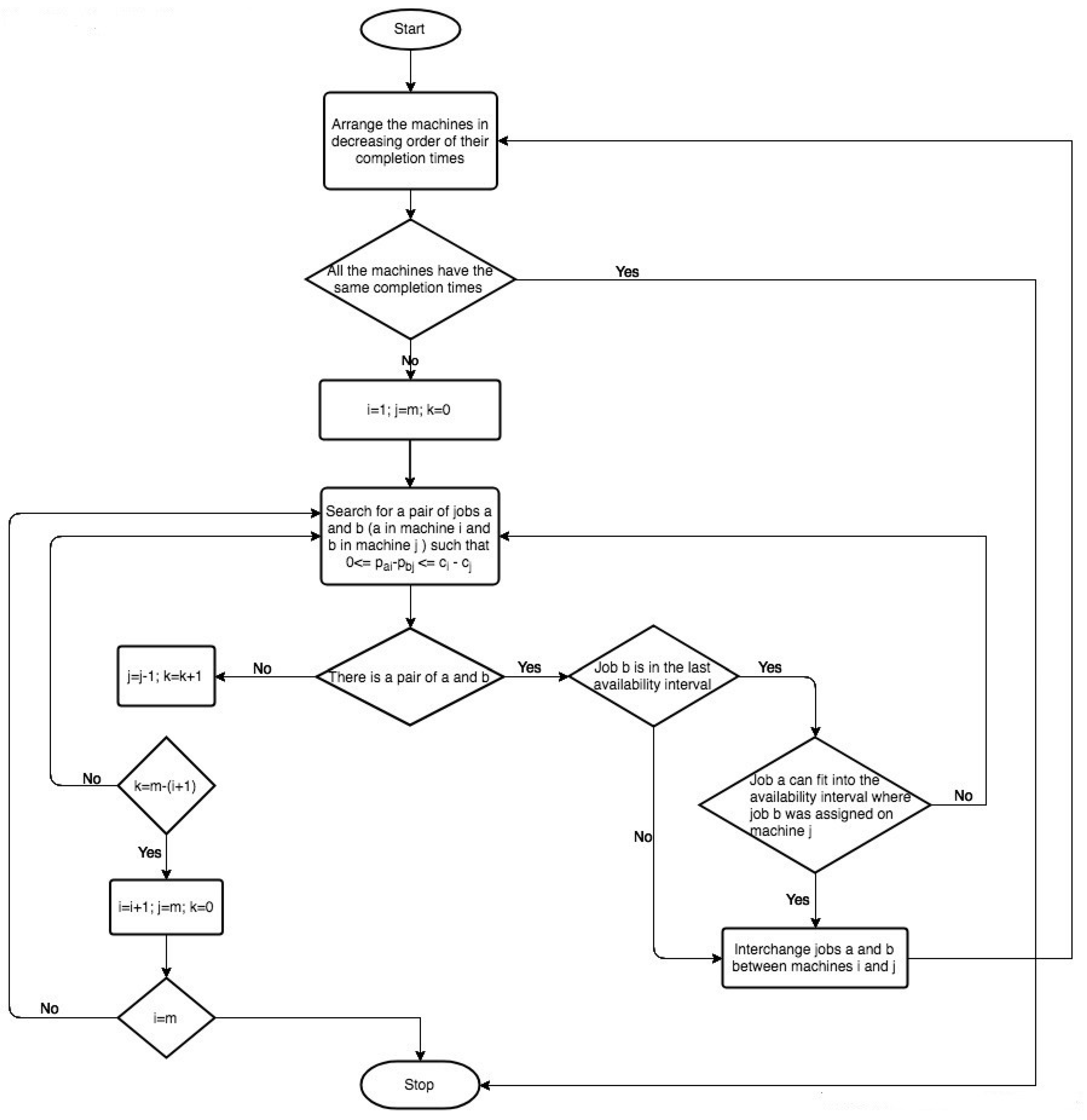
The idea of the improvement procedure was inspired from a local-search heuristic proposed in [16], developed to solve the scheduling problem of parallel identical-batch processing machines. The aim of the improvement procedure was to try to balance the load of different machines so that the completion times of the last jobs in every machine are almost the same. This improvement can be achieved by interchanging pairs of jobs between the most loaded machine and other machines. The flowchart of the aforementioned heuristic is shown in Figure 1.

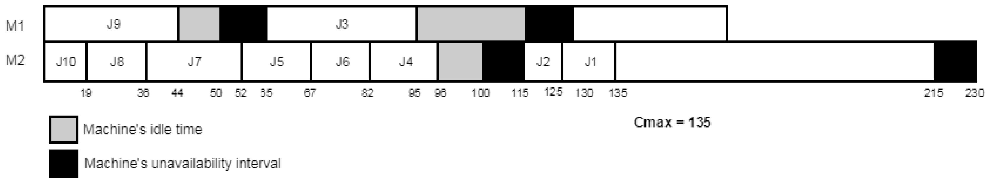
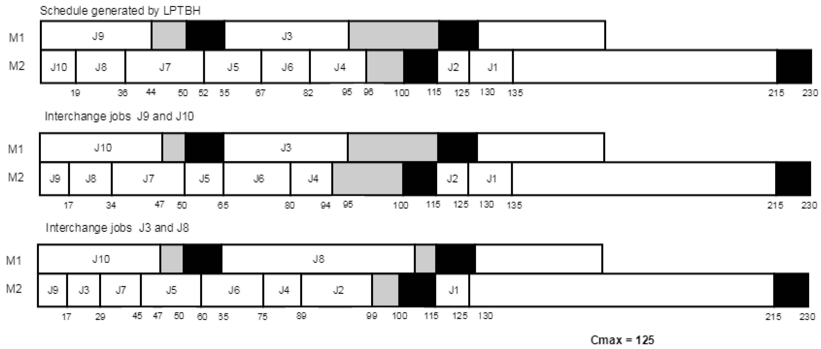
In order to illustrate the proposed heuristic, let us consider a problem instance with 2 machines and 10 jobs.

Table 2. Input data for 10 jobs and two machines.

Job j	1	2	3	4	5	6	7	8	9	10
$p_{1j}$	25	25	30	36	38	38	41	44	44	47
$p_{2j}$	10	10	12	14	15	15	16	17	17	19

summarizes the input data, and Figure 2 and Figure 3 show the Gantt charts of solutions obtained by $LPTBH$ and $LSHIP$, respectively.

Note that after interchanging a pair of jobs between two machines, the $LSHIP$ procedure looks to shift jobs to the left whenever the idle time interval on the machine can fit them. In the above example, after interchanging jobs $J3$ and $J8$, $LSHIP$ shifted job $J2$ to the left since it could fit in the idle time interval.

4. Experiment Results

For the purpose of evaluating the performance of the proposed algorithm, many problem instances were tested. These were generated after examining the important factors that significantly impacted the performance of the proposed algorithm. The first factor was the number of jobs n to be processed that directly affects the machines’ load. The second important factor is the number of machines m that has an impact on the assignment of jobs to machines. Job processing times may play a role in the efficiency of the proposed algorithm. Thus, we generated problem instances with different job processing times. The algorithm was coded in IntelliJ IDEA. In addition, the quadratic model was modelled in IBM ILOG CPLEX Optimization Studio 12.7. The proposed heuristic was implemented using programming language Java. We ran all test problems on an Intel Core i5 2.5 Gigahertz, 4 Gigabyte RAM Macintosh HD.

In order to avoid useless computational time, the program was stopped for two possible reasons. The first was when the CPLEX became unable to generate a solution within the time limit of 3600 s (1 h). The second reason was due to memory overflow. At this point, the best feasible solution found within the time limit was recorded.

4.1. Data Generation

A deep empirical study was conducted with the aim to generate datasets that would help to correctly analyze the efficiency of the proposed algorithm. By the end, two dataset series were considered, namely, $DS1$ and $DS2$. In fact, the way to generate dataset series $DS2$ was inspired from Graham’s data-generation process [17] addressing $P\left|\right|Cmax$ problems. The parameters used to generate $DS1$ and $DS2$ are summarized in

Table 3. $DS1$ parameters.

Number of machines (m)	$m\in \{2,3,5\}$
Number of jobs (n)	$n\in \{20,30,40,50,60,70,80\}$
Machine speed ($s_i$)	$s_i\in U(1,5)$
Job processing time ($p_j$)	$p_j\in U(5,50)$ and $p_j\in U(50,100)$
Number of unavailability periods ($n_i$)	$n_i=m\forall i=1,\dots ,m$
Duration of an unavailability period on machine i ($t_i$)	$t_i=10$, if $p_j\in U(5,50)$ and $t_i=15$, if $p_j\in U(50,100)\forall i=1,\dots ,m$
Length of time interval between two consecutive unavailability periods on machine i ($T_i$)	$Ti=25i$, if $p_j\in U(5,50)$ and $T_i=50i$, if $p_j\in U(50,100)$

and

Table 4. $DS2$ parameters.

Number of machines (m)	$m\in \{30,31,32,\dots ,\dots ,80\}$
Number of jobs (n)	$n=2m+1$
Machine speed ($s_i$)	$s_i\in U(1,5)$
Job processing time ($p_j$)	$p_j\in U(1,100)$
Number of unavailability periods ($n_i$)	$n_i=2\forall i=1,\dots ,m$
Duration of an unavailability period on machine i ($t_i$)	$t_i=10\forall i=1,\dots ,m$
Length of time interval between two consecutive unavailability periods on machine i ($T_i$)	$Ti=20i$

, respectively.

The starting and ending times $S_{ik}$ and $E_{ik}$ of the unavailability periods were generated according to Equations (9) and (10), respectively.

$$s_{ik}=k{T}_i+(k-1)t_{i}i=1,\dots ,m;k=1,\dots ,n_i$$

(9)

$$e_{ik}=s_{ik}+t_{i}i=1,\dots ,m;k=1,\dots ,n_i$$

(10)

4.2. Experiments

In this section, we outline different experiments that were conducted to evaluate the performance of the $QM$ and the proposed algorithm. In all experiments, Central Processing Unit time ($CPUt$) represents the time in seconds required to find the optimal or best feasible solution.

Table 5. Comparison of $QM$ and $MA$ for datasets $DS1$ with $s_i\in U(1,5)$ and $p_j\in U(5,50)$.

m	n	${\mathit{C}}_{\mathit{max}}\left(\mathit{QM}\right)$	${\mathit{C}}_{\mathit{max}}\left(\mathit{MA}\right)$	$\mathit{CPUt}\left(\mathit{QM}\right)$	$\mathit{CPUt}\left(\mathit{MA}\right)$
2	20	66	66	$1.16$	$0.01$
2	30	66	66	$1.16$	$0.01$
2	40	229	229	$0.46$	$0.02$
2	50	463	463	$0.86$	$0.05$
2	60	343	343	$1.26$	$0.03$
2	70	401	401	$0.71$	$0.04$
2	80	780	780	$1.25$	$0.03$
3	20	87	87	$1.72$	$0.01$
3	30	218	218	$3.58$	$0.04$
3	40	244	244	$3.91$	$0.02$
3	50	165	165	$2.81$	$0.02$
3	60	282	282	$4.73$	$0.02$
3	70	246	246	$4.01$	$0.04$
3	80	298	298	$6.46$	$0.04$
5	20	28	28	$1.52$	$0.02$
5	30	60	60	$3.25$	$0.03$
5	40	85	85	$7.24$	$0.03$
5	50	196	196	$114.24$	$0.06$
5	60	93	93	$1419$	$0.04$
5	70	120	120	$27.02$	$0.06$
5	80	174	174	$121.58$	$0.05$

and

Table 6. Comparison of $QM$ and $MA$ for datasets $DS1$ with $s_i\in U(1,5)$ and $p_j\in U(50,100)$.

m	n	${\mathit{C}}_{\mathit{max}}\left(\mathit{QM}\right)$	${\mathit{C}}_{\mathit{max}}\left(\mathit{MA}\right)$	$\mathit{CPUt}\left(\mathit{QP}\right)$	$\mathit{CPUt}\left(\mathit{MA}\right)$
2	20	169	169	$1.76$	$0.02$
2	30	409	409	$1.25$	$0.03$
2	40	319	319	$1.03$	$0.01$
2	50	622	622	$0.73$	$0.02$
2	60	567	567	$0.6$	$0.03$
2	70	659	659	$0.79$	$0.04$
2	80	689	689	$1.10$	$0.02$
3	20	130	130	$1.83$	$0.01$
3	30	239	239	$3.24$	$0.04$
3	40	359	359	$2.09$	$0.02$
3	50	365	365	$8.45$	$0.03$
3	60	407	407	$17.98$	$0.04$
3	70	561	561	$23.65$	$0.06$
3	80	702	702	$3.53$	$0.03$
5	20	94	94	$3.00$	$0.01$
5	30	143	143	$5.87$	$0.02$
5	40	277	277	$9.55$	$0.06$
5	50	272	272	$473.35$	$0.06$
5	60	208	208	$14.41$	$0.06$
5	70	382	382	$796.08$	$0.06$
5	80	339	339	$223.71$	$0.06$

show the results obtained by $QP$ and $MA$ for small and large job processing times, respectively.

Table 5 clearly shows that the proposed algorithm was generating optimal solutions with a $CPU$ time of less than 1 second for all problem instances. Quadratic model $QM$ was also able to provide optimal schedules in a reasonable time. By considering much longer processing times than in the previous data series, we still obtained optimal solutions in reasonable $CPU$ time even though the quadratic model became slower than in the first batch of problem instances. The proposed algorithm outperformed the quadratic model in terms of computational time that was still less than 1 second. Table 6 confirms these observations.

In order to investigate the limitations of the proposed quadratic model, a second dataset series, namely, $DS2$ was considered.

Table 7. Comparison of $QM$ and $MA$ for datasets $DS2$.

m	n	${\mathit{C}}_{\mathit{max}}\left(\mathit{QM}\right)$	${\mathit{C}}_{\mathit{max}}\left(\mathit{MA}\right)$	$\mathit{QP}$ Optimal?	$\mathit{CPUt}\left(\mathit{QM}\right)$	$\mathit{CPUt}\left(\mathit{MA}\right)$
30	61	133	133	Yes	$70.74$	$0.15$
33	67	137	137	Yes	$40.19$	$0.22$
36	73	142	142	Yes	$21.1$	$0.21$
40	81	140	140	Yes	$44.71$	$0.31$
45	91	232	232	Yes	$398.64$	$0.33$
51	103	240	240	Yes	$495.44$	$0.4$
57	115	237	237	Yes	$214.28$	$0.2$
62	125	336	336	Yes	$263.21$	$0.2$
68	137	331	331	Yes	$393.97$	$0.39$
73	147	434	434	No	$3603.54$	$0.42$
76	153	439	439	No	$3602.48$	$0.43$
80	161	538	538	Yes	$3602.9$	$\mathrm{0.0.27}$

reports the computational results for both $QM$ and $MA.$

The computational results displayed in Table 7 show that quadratic model $QM$ was able to generate an optimal solution within a time limit for problems with up to 73 machines.

On the basis of the computational results shown in Table 7, the quadratic model was not able to generate optimal solutions in a reasonable time and for bigger problems. Therefore, proposed procedure $MA$ was tested for large-sized problems and compared to an adapted form of $MLPT$, proposed earlier by the author of this paper in [7].

Table 8. Comparison of $MA$ and $MLPT$.

m	n	${\mathit{C}}_{\mathit{max}}\left(\mathit{MLPT}\right)$	${\mathit{C}}_{\mathit{max}}\left(\mathit{MA}\right)$	${\mathit{C}}_{\mathit{max}}\left(\mathit{MLPT}\right)/{\mathit{C}}_{\mathit{max}}\left(\mathit{LSHIP}\right)$	$\mathit{CPUt}\left(\mathit{QP}\right)$	$\mathit{CPUt}\left(\mathit{MA}\right)$
100	201	1120	880	$1.27$	$0.47$	$0.49$
200	401	1090	1050	$1.03$	$2.16$	$2.5$
300	601	1250	970	$1.28$	$4.69$	$4.81$
400	801	1110	960	$1.15$	$9.12$	$9.55$
500	1001	1120	760	$1.47$	$16.24$	$15.48$
600	1201	1260	1240	$1.01$	$28.24$	$24.07$
700	1401	1240	1160	$1.06$	$41.92$	$62.24$
800	1601	1260	1110	$1.13$	$74.97$	$48.5$
1000	2001	1110	1080	$1.02$	$120.04$	$122.99$

reports the obtained results for problem instances with $m\in \{100,200,300,400,500,600,700,800,1000\}$ and $n=2m+1.$

Table 8 shows that $MA$ outperformed $MLPT$ for all problem instances with slightly higher $CPU$ time than the time of $MLPT$$CPU$ for most instances. In addition, run time increased with problem size.

5. Conclusions and Future Work

In this paper, we studied the problem of parallel machine scheduling with multiple planned nonavailability periods. In the current literature, very few papers investigated this problem. The problem was formulated as a quadratic program and optimally solved using CPLEX for small- to moderately large-sized problems. In order to be able to solve large-sized problems, an algorithm consisting of two main phases was developed. The first phase searches for schedules on the basis of the $LPT$ rule. The second aims to improve these schedules by considering simultaneous pairwise interchanges of jobs between machines. A deep computational study was conducted to test the efficiency of the proposed approach. Many datasets were carefully generated to help evaluate the algorithm. Computational results showed that the proposed algorithm generated optimal solutions for all considered problem sizes and outperformed an adapted form of a heuristic that was developed earlier by the author of this paper. Further investigation can be done to consider other criteria and more general versions of the problem, such as the dynamic case where jobs arrive one by one over the planning horizon.

References

- Azadeh, A.; Sheikhalishahi, M.; Firoozi, M.; Khalili, S. An integrated multi-criteria Taguchi computer simulation-DEA approach for optimum maintenance policy and planning by incorporating learning effects. Int. J. Prod. Res. 2013, 51, 5374–5385. [Google Scholar] [CrossRef]
- Yazdani, M.; Khalili, S.M.; Jolai, F. A parallel machine scheduling problem with two-agent and tool change activities: An efficient hybrid metaheuristic algorithm. Int. J. Comput. Integr. Manuf. 2016, 29, 1075–1088. [Google Scholar] [CrossRef]
- Azadeh, A.; Sheikhalishahi, M.; Khalili, S.M.; Firoozi, M. An integrated fuzzy simulation—Fuzzy data envelopment analysis approach for optimum maintenance planning. Int. J. Comput. Integr. Manuf. 2014, 27, 181–199. [Google Scholar] [CrossRef]
- Low, C.; Ji, M.; Hsu, C.J.; Su, C.T. Minimizing the makespan in a single machine scheduling problems with flexible and periodic maintenance. Appl. Math. Model. 2010, 34, 334–342. [Google Scholar] [CrossRef]
- Schneider, M.; Stenger, A.; Hof, J. An adaptive VNS algorithm for vehicle routing problems with intermediate stops. Or Spectrum 2015, 37, 353–387. [Google Scholar] [CrossRef]
- Graham, R.L.; Lawler, E.L.; Lenstra, J.K.; Kan, A.R. Optimization and approximation in deterministic sequencing and scheduling: A survey. Ann. Discrete Math. 1979, 5, 287–326. [Google Scholar]
- Kaabi, J.; Harrath, Y. Scheduling on uniform parallel machines with periodic unavailability constraints. Int. J. Prod. Res. 2019, 57, 216–227. [Google Scholar] [CrossRef]
- Liu, M.; Zheng, F.; Chu, C.; Xu, Y. Optimal algorithms for online scheduling on parallel machines to minimize the makespan with a periodic availability constraint. Theor. Comput. Sci. 2011, 412, 5225–5231. [Google Scholar] [CrossRef]
- Liao, L.W.; Sheen, G.J. Parallel machine scheduling with machine availability and eligibility constraints. Eur. J. Oper. Res. 2008, 184, 458–467. [Google Scholar] [CrossRef]
- Mellouli, R.; Sadfi, C.; Chu, C.; Kacem, I. Identical parallel-machine scheduling under availability constraints to minimize the sum of completion times. Eur. J. Oper. Res. 2009, 197, 1150–1165. [Google Scholar] [CrossRef]
- Fu, B.; Huo, Y.; Zhao, H. Approximation schemes for parallel machine scheduling with availability constraints. Discret. Appl. Math. 2011, 159, 1555–1565. [Google Scholar] [CrossRef]
- Wang, X.; Cheng, T. A heuristic for scheduling jobs on two identical parallel machines with a machine availability constraint. Int. J. Prod. Econ. 2015, 161, 74–82. [Google Scholar] [CrossRef]
- Gedik, R.; Rainwater, C.; Nachtmann, H.; Pohl, E.A. Analysis of a parallel machine scheduling problem with sequence dependent setup times and job availability intervals. Eur. J. Oper. Res. 2016, 251, 640–650. [Google Scholar] [CrossRef]
- Lee, C.Y. Parallel machines scheduling with nonsimultaneous machine available time. Discret. Appl. Math. 1991, 30, 53–61. [Google Scholar] [CrossRef]
- Mireault, P.; Orlin, J.B.; Vohra, R.V. A parametric worst case analysis of the LPT heuristic for two uniform machines. Oper. Res. 1997, 45, 116–125. [Google Scholar] [CrossRef]
- Kashan, A.H.; Karimi, B.; Jenabi, M. A hybrid genetic heuristic for scheduling parallel batch processing machines with arbitrary job sizes. Comput. Oper. Res. 2008, 35, 1084–1098. [Google Scholar] [CrossRef]
- Graham, R.L. Bounds on multiprocessing timing anomalies. SIAM J. Appl. Math. 1969, 17, 416–429. [Google Scholar] [CrossRef] [Green Version]
Figure 1.
Flowchart of procedure.
Figure 2.
Gantt chart of solution generated by .
Figure 3.
Gantt chart of the solution generated by .