Walking Gait Phase Detection Based on Acceleration Signals Using LSTM-DNN Algorithm

College of Engineering, Beijing Forestry University, Beijing 100083, China
*
Author to whom correspondence should be addressed.
Algorithms 2019, 12(12), 253; https://0-doi-org.brum.beds.ac.uk/10.3390/a12120253
Submission received: 14 October 2019
/
Revised: 8 November 2019
/
Accepted: 23 November 2019
/
Published: 26 November 2019
(This article belongs to the Special Issue Algorithms for Pattern Recognition)
Abstract
:Gait phase detection is a new biometric method which is of great significance in gait correction, disease diagnosis, and exoskeleton assisted robots. Especially for the development of bone assisted robots, gait phase recognition is an indispensable key technology. In this study, the main characteristics of the gait phases were determined to identify each gait phase. A long short-term memory-deep neural network (LSTM-DNN) algorithm is proposed for gate detection. Compared with the traditional threshold algorithm and the LSTM, the proposed algorithm has higher detection accuracy for different walking speeds and different test subjects. During the identification process, the acceleration signals obtained from the acceleration sensors were normalized to ensure that the different features had the same scale. Principal components analysis (PCA) was used to reduce the data dimensionality and the processed data were used to create the input feature vector of the LSTM-DNN algorithm. Finally, the data set was classified using the Softmax classifier in the full connection layer. Different algorithms were applied to the gait phase detection of multiple male and female subjects. The experimental results showed that the gait-phase recognition accuracy and F-score of the LSTM-DNN algorithm are over 91.8% and 92%, respectively, which is better than the other three algorithms and also verifies the effectiveness of the LSTM-DNN algorithm in practice.
1. Introduction
Event detection in the medical field has been a trend in gait event detection in recent years [1]. Gait analysis is of great help to therapists who wish to monitor the recovery of patients going through rehabilitation processes [2]. As of 2007, there were an estimated 1.1 million children with gait disorders in the United States and the likely reasons are different somatosensory diseases [3]. Gait phase detection is an effective method to detect the morbid phases [4,5] and has great significance for the clinical rehabilitation of patients. In addition, researchers have managed to program humanoid robots to use human-based gait trajectories generated via gait classification [6], as well as consistently control wearable assistive devices such as robotic prostheses [7] and orthoses [8] for the recovery of lower-limb mobility. For instance, Yan et al. [9] proposed that gait phase detection can also be used to facilitate the development of human auxiliary equipment, such as medical ankle joint (AF), hip joint (HK), and knee ankle joint (KAF) orthopedic devices, as well as exoskeletons and other equipment.
In terms of gait division, the gait phase is mainly divided into a standing phase and a swing phase. Among them, standing phase class is subdivided into initial contact (IC), flat foot (FF), and heel-off (HO). Juri et al. [10] proposed the division of the gait cycle into several phases, namely initial contact (IC), flat foot (FF), heel-off (HO), and the initial swing phase (SP). This division of gait phase is very detailed, but it also brings certain difficulties to the detection. Besides, a two-phase model has proven to be sufficient to control the knee module of an active orthosis [11]. In other words, the gait phase is divided into standing phase and swing phase.
Currently, there are mainly two types of sensors for phase detection, namely wearable sensors and non-wearable sensors. Non-wearable sensors mainly contain gait phase detection based on machine vision. Machine vision primarily refers to vision systems such as web cameras. Wearable sensors mainly contain pressure sensors [12], acceleration sensors [13], etc. In addition, the EMG sensor [14] can be used to indirectly detect gait events. This type of sensor time is popular because they are easy to wear and inexpensive. At present, the foot pressure sensor is widely used, in addition to the above advantages, but also because each gait phase can correspond to different pressure modes [15]. The plantar pressure sensor is small and can be easily installed in the insole. In addition, the plantar pressure sensor is a force-sensitive resistor (FSR) whose resistance can vary with pressure. However, the plantar pressure sensor needs to be accurately mounted at the designated location [16], which requires subjects with different shoe sizes to wear the appropriate insole. This will undoubtedly increase the cost of the study. In this case, as the level of sensor technology increases, the use of inertial sensors to detect gait phase is becoming more widespread. The use of inertial sensors is also due to the fact that the acceleration signal exhibits typical waveform characteristics in the gait cycle [12], with which we can detect specific phases. In this study, we utilized the acceleration sensor to detect the gait phase and achieve a better recognition effect.
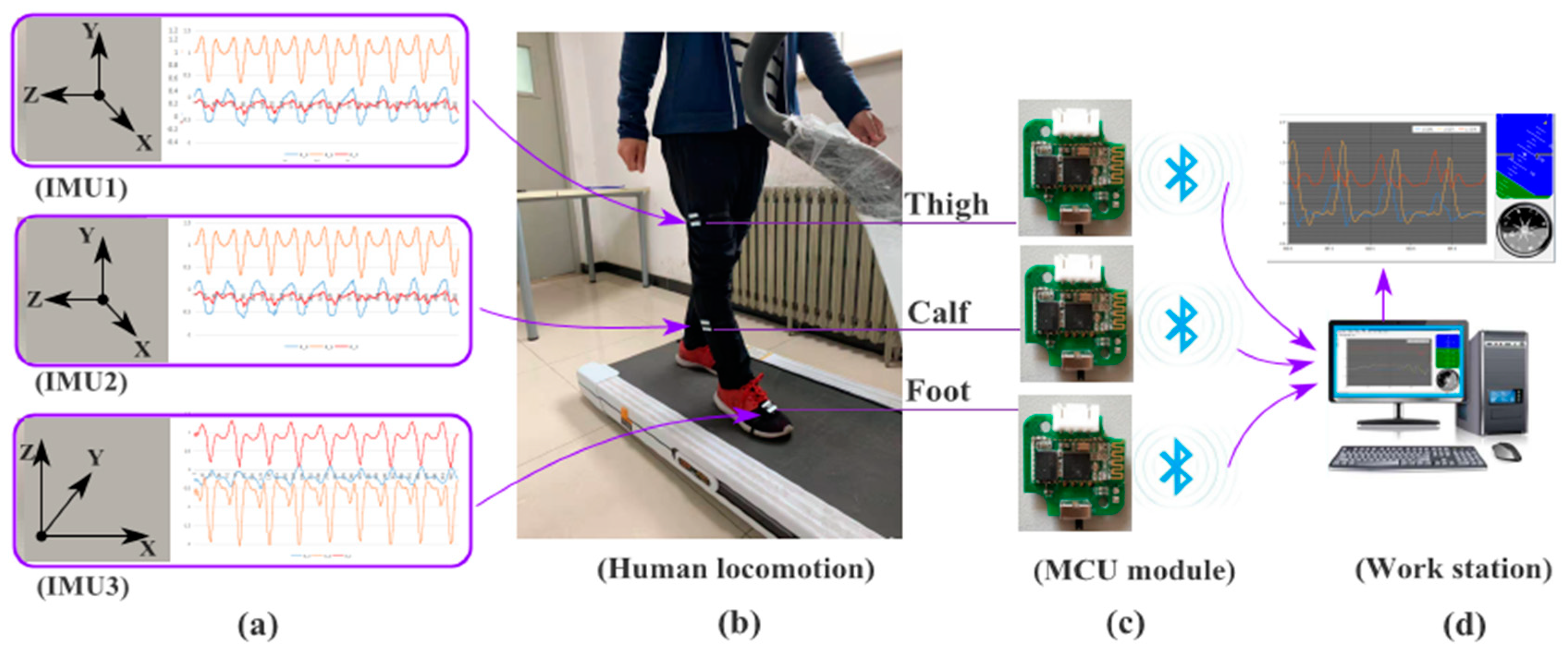
Previous studies have positioned inertial sensors on the instep [17], thigh [18], and calf [19]. In view of previous studies and to further improve the effectiveness of gait event monitoring, this paper considers the position of the instep, lower leg, and thigh because the classifier has better classification performance at the lower extremity position [20]. When the speed sensor is installed in these three body parts, it can continuously output different periodic signals, which is the basis for the gait phase division by the acceleration signal.
The study presented here features a gait phase detection system that utilizes inertial motion data from three acceleration sensors to detect two gait phases by means of four detection algorithms. Based on the comparison between the performance of the deep learning algorithm and the machine learning method, the input values of the two types are derived from the acceleration data of three different body parts, revealing which algorithm is more suitable for the gait phase detection system.
2. Related Works
Computational methods for gait phase recognition fall into two main categories. The first category is comprised of algorithms, which divide the gait phases based on the threshold selection of either raw or processed data [21]. Secondly, some deep-learning approaches have emerged in recent years to substitute the aforementioned techniques that relay traditional classification algorithms. Some have applied deep learning algorithms to different types of sensors to detect gait phases. For instance, Mukherjee et al. [22] present a fully automated frontal (i.e., employing front and back views only) gait phase recognition approach using the depth information captured by multiple Kinect RGB-D cameras. However, the captured image information is easily disturbed by the external environment. Rosati et al. [14] proposed a method of hierarchical clustering to achieve recognition of human gait phase by processing electromyography (EMG) data collected during gait, which has improved the above-mentioned problems that are susceptible to environmental interference. However, muscle electrical signals are susceptible to factors such as sweat when collecting EMG data. Ding et al. [23] further improved the problems of the above EMG method, and proposed a proportional fuzzy (PBF) algorithm to achieve smooth recognition of gait phase for foot pressure information processing, but the foot pressure will be affected by the wearer’s weight, load, and other factors [19]. For participants with large differences in weight, we need to constantly recalibrate the threshold of the pressure sensors. Besides, the pressure sensor constantly rubs in the middle of the insole, thereby shortening its life [24]. Therefore, the use of whole inertial measurement units (IMU) has risen lately. This is mainly due to the fact that more information can be obtained by adopting a small number of inertial sensor modules, and most of the inertial sensor modules are installed on the legs and feet, so as to avoid damage or discomfort to the wearer [25]. At the same time, the information of IMU is basically unaffected by human body weight, sweat, and other factors, which is a prominent advantage compared to the method of plantar pressure or muscle electrical signal detection. In addition, inertial sensors are extremely cost-effective [26], and the acceleration signals acquired by inertial sensors exhibit typical waveform characteristics during the gait cycle [27]. More recently, the use of this type of sensor to collect movement data has increased rapidly [28]. Previous studies have also used acceleration to detect gait time practice [29], but there are few studies using acceleration sensors to detect gait phase.
This paper builds a system that uses three inertial sensor modules to obtain the acceleration information of the lower limbs of the human body. The collected acceleration data was reduced by the principal components analysis (PCA) algorithm, which focuses on extracting the feature information of the original data and searches for a set of orthogonal low-wiki functions to represent a set of high-dimensional data, improving the recognition rate and recognition speed [30]. Then the paper divides the human gait into two phases and proposes a method of dividing the two gait phases. Finally, this paper proposes a LSTM-DNN algorithm for detecting gait phase. The designed LSTM-DNN with higher accuracy will be further evaluated with learned and unlearned data to test its suitability with acceleration classification.
For the recognition system, this paper designs an effective and adaptable gait detection method. Foreign research results [19] indicate that a large amount of information can be obtained by using a small number of acceleration sensors that are located on the legs and feet to minimize sensor damage and discomfort to the person wearing the sensor. In this study, a speed sensor data acquisition device is developed to obtain gait information for human lower limbs for gait detection. Principal components analysis (PCA) is used to preprocess the data and an LSTM-DNN algorithm is proposed to detect the gait phases. The PCA algorithm extracts the feature information of the original data. A set of orthogonal functions is used to represent the high-dimensional data to improve the recognition rate and speed [30,31,32].
This paper proposes an algorithmic model for detecting gait phase, which uses the acceleration data from the instep, calf, and thigh to accurately detect two gait phase events. Finally, the effectiveness of the proposed LSTM-DNN algorithm in gait phase detection is verified by the final recognition results.
3. Materials and Methods
3.1. Data Collection
In the experiments, we recruited four undergraduate students (one female, three male) for the experiment. The participants were 20 to 23 years old, weighed 45 kg to 75 kg, and were between 155 cm and 180 cm tall. Participants were able to walk normally and had no conditions that affected their gait.
The wearable sensors were triaxle acceleration sensors. Due to the improvement of the sensor manufacturing process and optimized detection algorithms, more data can be obtained today using fewer sensors [33], which is one of the important reasons why inertial sensors are increasingly used in gait events in recent years.
The acceleration sensors were placed on the foot instep [34], calf [19], and thigh [18]. The direction of the acceleration sensor on the instep, calf, and thigh is shown in Figure 1a. The acceleration resolution of the three-axis accelerometer was 6.1 × 10⁻⁵g, the attitude measuring stability was 0.01°, and the baud rate range was 2400–921,600 bps. The baud rate used in the experiment was 115,200 bps and the sampling frequency was 50 Hz.
The toggle switch of the triaxial acceleration sensor was used to collect the acceleration data. Participants were then asked to walk for at least 120 s on the already configured treadmill. In addition, the treadmill speeds were set at 0.78 m/s, 1.0 m/s, and 1.25 m/s, respectively. Participants walked normally three times on a treadmill at each speed, with all settings being the same in each state. In order to prevent the participants from affecting the gait due to fatigue, the experiment requires the participants to rest for 2 min for each walking test. In addition, we only start saving data when the treadmill’s running speed reaches the set speed. Similarly, when the experiment was stopped and the treadmill began to slow down, we stopped collecting data. Moreover, each participant was asked to perform the same experiment under the same conditions to ensure the reliability and validity of the collected data.
3.2. Data Preprocessing
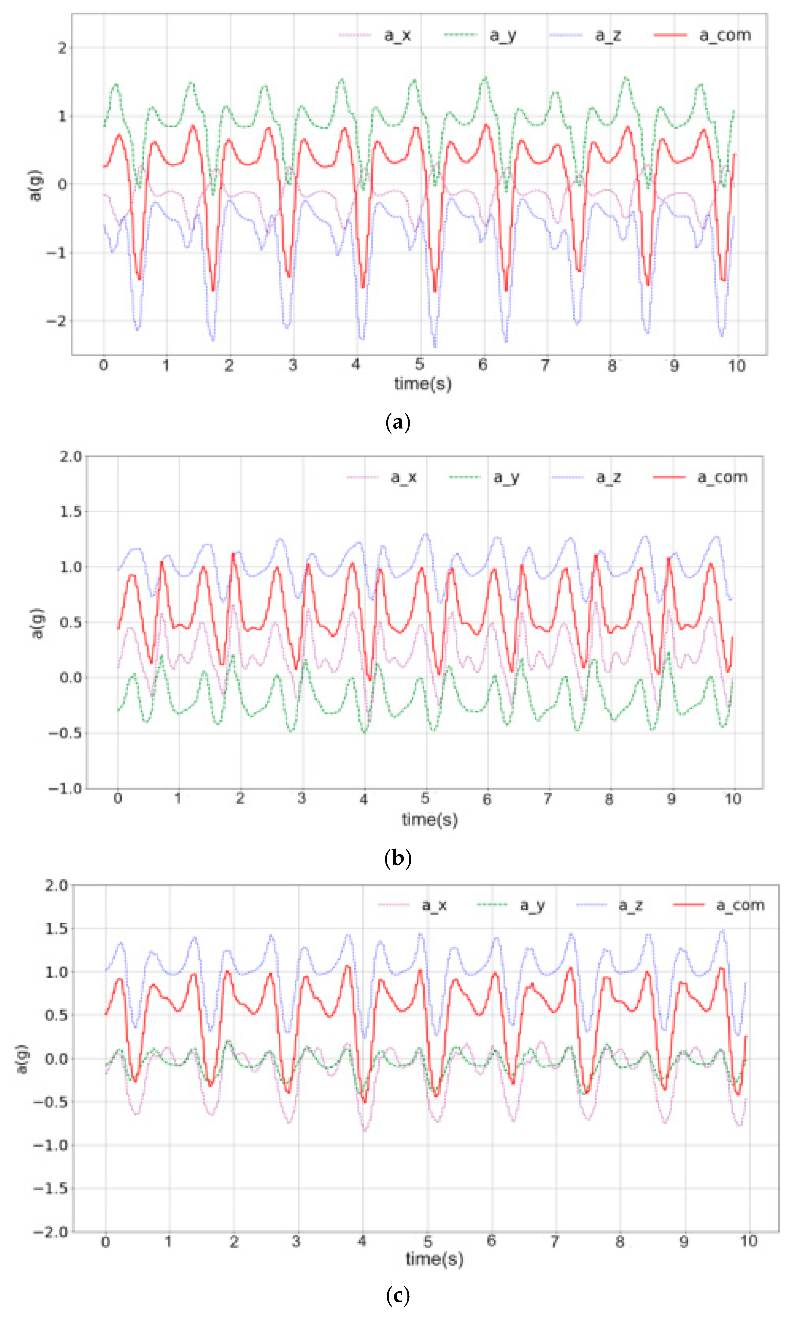
Because each dataset has multiple characteristics and includes the acceleration in the X-, Y-, and Z-directions, a large number of features would result in large complexity of the DNN model. PCA uses dimensionality reduction and transforms multiple indices into a few comprehensive indices (principal components). The principal components contain most of the information of the original variables and the information in the principal components is not correlated. This method reduces many complex factors into several principal components, which simplifies the problem. In this study, PCA was used to compress the data and generate a synthetic variable Comp. Comp is expressed by Equation (1), where , and represent the acceleration in the X-, Y-, and Z-directions respectively, and z1, z2, and z3 represent the coefficients of the acceleration in three directions, respectively. The distribution of z1, z2, and z3 corresponding to different body parts at asynchronous speed is shown in Table 1. In the walking experiment, the acceleration and composite acceleration data curves of the three directions collected are shown in Figure 2.
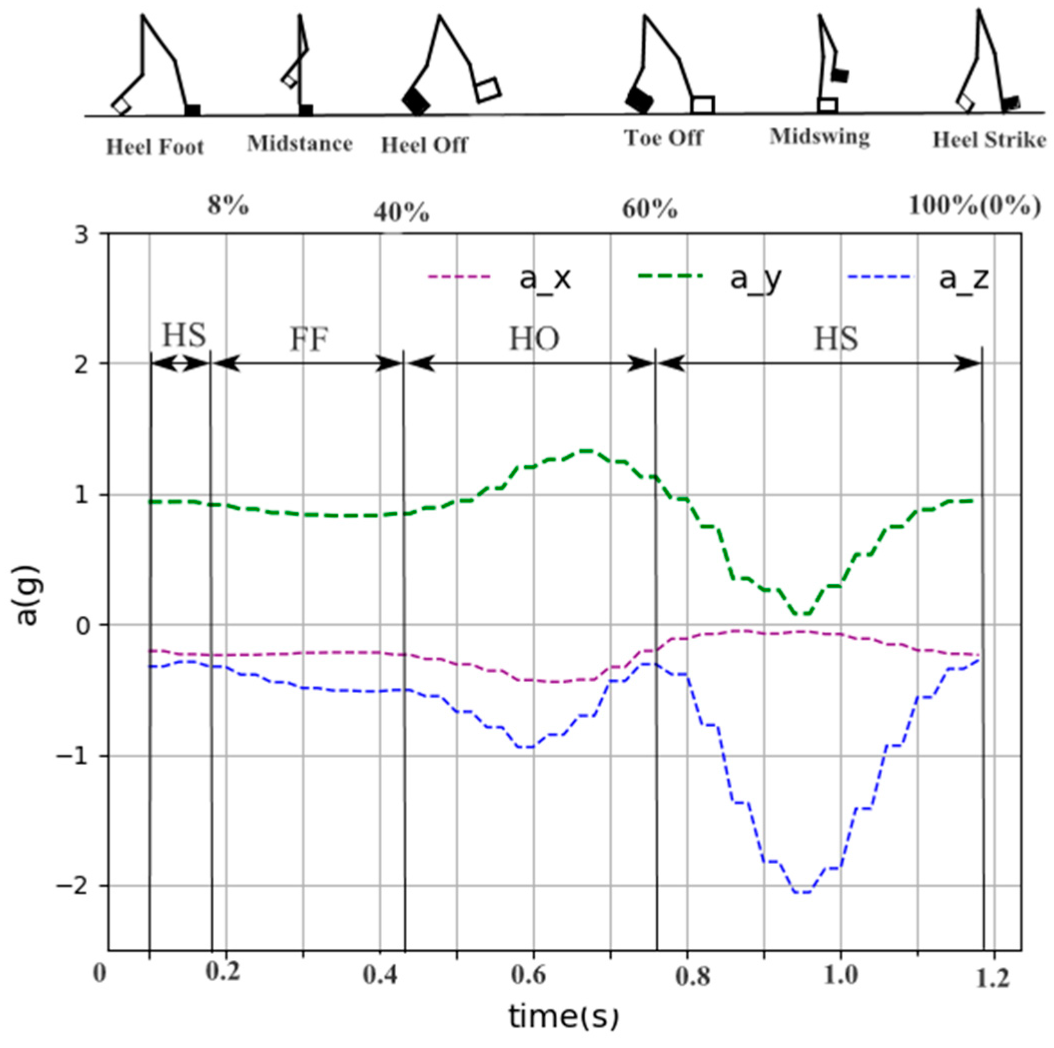
During normal walking, the acceleration signals in the three directions of the foot, thigh, and calf exhibit periodicity. The sway phase accounts for approximately 40% of the total gait phase, and the stance phase accounts for approximately 62% of the total gait phase [35]. We can approximate that the stance phase is the biggest phase in the walking cycle. Determined according to the division of gait phase by Miguel et al. [27], the phase division in this paper is shown in Figure 3. Feature extraction is used to extract meaningful information or noise from acceleration graphs. After processing, the corresponding gait phase is obtained by using a classification algorithm.
On a related note, feature extraction is an effective and important method in extracting meaningful information from acceleration signals. The extracted features used in this study include the standard deviation (SD), mean absolute value (MAV), maximum (MAX), minimum (MIN), and median (MED). These features were selected because some of them were used in the study by Miguel et al. on acceleration signals [27].
Su et al. [36] proposed the use of single and multiple feature sets to achieve high accuracy. Therefore, to assess multi-feature performance and improve recognition accuracy, SD, MAX, MIN, MED, and MAV were combined to create the input feature vector. Because PCA was performed for dimensionality reduction, the number of input eigenvectors for the neural network is relatively low.
3.3. Gait Phase Division
A person’s walking process is a rhythmic movement and a complete walking cycle consists of following the ground with one foot to landing again with the same heel [35]. During the walking cycle, the legs support the body’s weight during forward movement. Taborri et al. [11] divided the gait phase into four phases, which comprises: (i) heel strike (HS); (ii) flat foot (FF); (iii) heel-off (HO); and (iv) swing phase (SW). This phase division is relatively detailed and makes the system more complex, thereby potentially lowering the recognition accuracy. Mileti et al. [37] divided the gait cycle into four phases, namely, loading response (LR), flat-foot (FF), pre-swing (PS), and swing (SW) for the analysis, but there is a large error in the SW phase and the PS phase. Therefore, in order to improve the recognition accuracy, it is usually necessary to use fewer divisions. Most researchers tend to group this cycle into stance and swing phases [16]. By referring to the above classification of gait, and ensuring the scientificity of the classification of gait, it is decided to divide the walking cycle into the stance and swing phases. Among them, the standing posture mainly includes HS, FF, and HO phases. The gait phase division is shown in Figure 3. The first 60% of the signal of a complete cycle belongs to the stance phase, and the next 40% of the signal belongs to the swing phase.
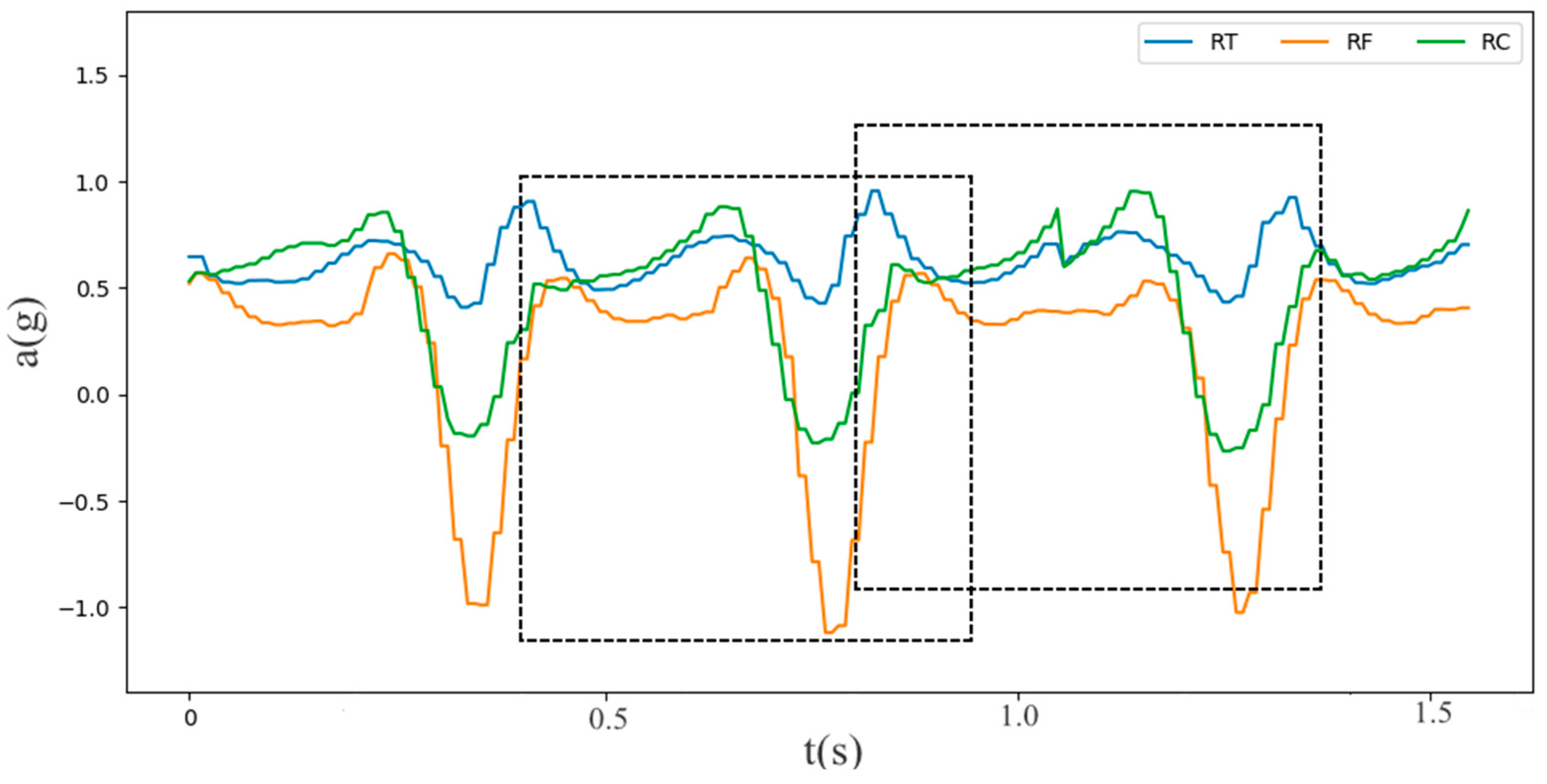
Then we need to split the data. The data collected by the inertial sensor is a data stream distributed over time. It is not possible to directly extract and classify the features, and the data needs to be segmented. At present, the method of data segmentation is a multi-dimensional sliding window segmentation method [38]. The acceleration signal is divided into sections with different gait phase information by using a sliding window segmentation method. The sliding windows are divided into overlapping windows and separated windows. Overlapping windows usually minimize the influence of the transition process on the detection accuracy [39]. Therefore, a window with a 50% overlap is used in most studies [38]. The sliding window uses a 50% coverage period to evaluate the gait phase. Figure 4 shows a schematic diagram of the sliding window segmentation.
3.4. Proposed LSTM-DNN Algorithm
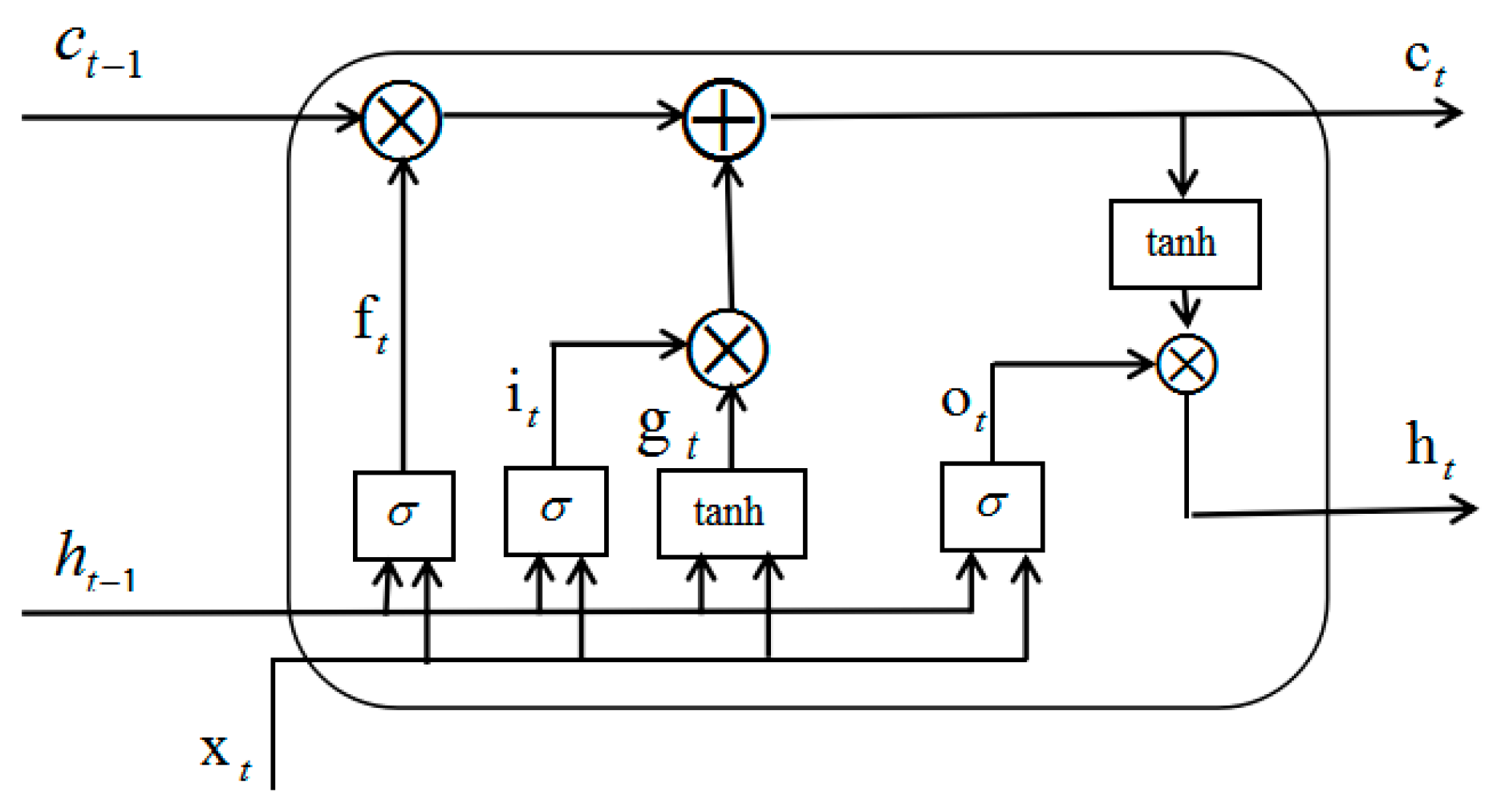
LSTM network is proposed based on a cyclic neural network (CNN). Hochreiter et al. [40] proposed the LSTM network by adding thresholds such as an input gate, forget gate, output gate, and memory unit, which solved the problem of gradient disappearance or gradient explosion of the RNN and improved the network’s ability to process long sequence data. The difference between LSTM and an ordinary neural network is that the nodes between the hidden layers are connected, i.e., the input of the hidden layer at the given time not only contains the output of the hidden layer prior to the given time but also includes the output of the same hidden layer at a previous time. The historical information of the time series is stored in the network hidden layer [41].
The LSTM can be utilized to process sequence data. Since the acceleration signal we collect is a time-series signal, the LSTM network can be utilized to process the acceleration signal. Unlike traditional classifiers such as SVM, the LSTM can capture feature vectors conveniently and automatically. The feature vectors enter the network directly and a modified classification model is established, whereas a traditional classification model requires more time to extract the feature vectors, leading to possible failure in the data preprocessing stage [42].
The LSTM algorithm model is shown in Figure 5 [43], where is the input eigenvector of the current cell, is the output of the last cell, sigma is the sigmoid function, is the forget gate for information to be abandoned, is the unit before the update, and the output value of is a real number between 0 and 1; 0 means to forget all the information of the previous cell unit and 1 means to retain all the information of the previous cell unit and input the output value to . The calculation process of the forget gate is defined in Equation (2); the information is discarded when the input information passes through the forget gate. The input gate consists of two parts, i.e., a sigmoid layer and the tanh layer. The sigmoid layer is responsible for information that requires updating and the tanh layer is responsible for creating the vector of the alternative update content; these two parts are combined and represent the output of the output gate. The calculation is defined in Equation (3) and Equation (4). After the information passes through the forget gate and input gate, the cell state will be updated. The calculation is defined in Equation (5); the old status is updated to . Finally, the output gate also includes a sigmoid layer and a tanh layer. The sigmoid layer determines which input information needs to be output and the tanh layer processes the information of the cell state and combines the two parts as the output of the output gate. The calculation process is shown in Equations (6) and (7), where represent the weights of the input of the current eigenvector through each control gate and represent the bias terms of the control gate.
DNN algorithms have been widely used in industry and academia in recent years. The DNN algorithm provides good recognition rates. As an important machine learning method, a DNN performs particularly well for multi-label classification [44]. This study focuses on the identification of two classes, namely, the stance phase and swinging phase. The training data set contains five features extracted from the subjects’ gait events.
The DNN is a feed-forward artificial neural network consisting of an input layer, an output layer, and at least two hidden layers [45]. Several important parameters need to be set, including the gradient descent optimizer, learning rate, activation function, and training steps. In most machine learning tasks, the objective is to minimize loss and, in the case of loss definitions, the subsequent task is to select and define the optimizer. Gradient optimization is a common method of deep learning, that is to say, the optimizer is actually the optimization of the gradient descent algorithm at the end. The optimizer chosen in this study is the AdaGrad algorithm. The original gradient descent optimization algorithm converges slowly near the bottom of a slope but this is avoided when the AdaGrad algorithm is used. Because of the steep directional gradient, the learning rate will decay faster, which is conducive to the parameter moving in the direction closer to the bottom of the slope, thus accelerating the convergence [46].
The learning rate has a crucial influence on the learning quality of the established learning model. The smaller the learning rate, the more sophisticated the learning is but at the same time the learning speed is also reduced, which will easily cause overmeshing and reduces the generalization ability of the training model. Similarly, if the learning rate is too high, the span of each step is too large and the model will miss a lot of important information in the training process, resulting in poor detection accuracy of the training model [47]. The learning rate is generally related to the selected optimizer, the neural network model, the number of training steps, and the size of the sample set. In the LSTM-DNN algorithm, the learning rate is 0.001, 0.003, 0.005, 0.008, 0.01, 0.05, 0.08, 0.1, 0.03, 0.5, 0.7, and 0.8, respectively. Finally, when the learning rate is 0.5, each evaluation index is relatively high. There are three multi-label hidden layers. In a multilayer neural network, there is a functional relationship between the output of the upper node and the input of the lower node, which is called the activation function. In this study, the ReLu function is used as the activation function of the neurons. The important feature of AdaGrad algorithm, which is used as the optimizer, is that it automatically adjusts the learning rate, thereby avoiding the occurrence of the dead ReLu problem caused by a very large learning rate. The softmax classifier is an extension of the logistic regression model for multi-classification problems. For multi-classification, the softmax function is generally used for the activation function of the output layer [42]. For multi-classification problems, it is evident from Equation (8) that the softmax function maps the output of multiple neurons to the interval of (0,1). When selecting the output node, we can select the node with the highest probability as the prediction target of the model, thus achieving multi-classification.
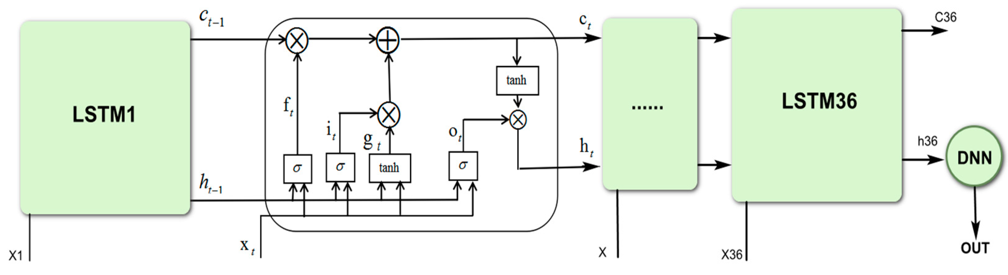
The acceleration signal obtained in this study is a time series signal; therefore, it can be input directly into the LSTM network for preprocessing. The LSTM network output layer signal represents the input into the DNN; the DNN improves the LSTM network output signal, resulting in greater accuracy. The structure of the LSTM-DNN is shown in Figure 6. The pre-processed data consisted of 18 parameters and a total of 198,930 learning data point were calculated with the LSTM-DNN algorithm. The LSTM network includes two important parameters, i.e., num_units and forget_bias. Num_units refers to the number of neurons in a cell and forget_bias refers to the bias in the forget gates. In this study, there are 36 num_units and the forget_bias is 0.7. In addition, the LSTM-DNN algorithm used in this study is also a multi-layer perceptron with a DNN basic architecture network. The feed-forward DNN has five layers, namely one input layer, two hidden layers, and one output layer. In general, the input vector P of the input layer is expressed as p1, p2, ..., p15 and each input is represented by the corresponding weight matrix w11, w21, and w181. The essence of the LSTM-DNN algorithm is to integrate the DNN and LSTM network. Although the LSTM-DNN algorithm performs better in timing signal processing, it has a simple network structure due to fewer neurons. In the training process, the predicted value of the DNN is fed back to the LSTM network continuously. Since the DNN is used, the weights of the LSTM network and the DNN change during the training process. As a result, the fluctuations in the weight of the LSTM network in the later training process are reduced, thereby stabilizing the network structure. First, the LSTM network processes the output of the previous cell and the input eigenvectors of the current cell. Then the DNN uses the LSTM network’s output signal as the input signal and the weights are adjusted in the DNN and the LSTM network through the training process. Finally, the trained network structure is used and the classification is conducted using the Softmax classifier gait detection.
We compared the results of the LSTM-DNN with those of more mature and traditional algorithms, namely, the k-nearest neighbor method (KNN) and SVM, which are installed in the sklearn package. In order to make the classification results have certain comparability, this paper also uses the PCA processed data set as the input of KNN and SVM classifier. SVM algorithms separate classes into different class hyperplanes using samples. The algorithm maximizes the distance between two samples, thus differentiating the categories as much as possible. Among them, the choice of kernel function is crucial to the performance of the support vector machine algorithm. The kernel functions of support vector machines mainly include linear kernel function, RBF kernel function, poly kernel function, and sigmoid kernel function. In order to determine the kernel function under the unsynchronized speed, this paper has introduced these four kinds of kernel functions and tested them separately, and obtained the results as shown in Table 2. In the KNN classification algorithm, if most of the K closest samples in the feature space belong to a certain category, the samples also belong to this category. The KNN algorithm is suitable for multi-classification. The KNN distance parameter chosen in this paper is the euclidean distance. In addition, the use of the KNN algorithm involves the parameter K. In order to find the ideal K value, the paper takes the values of 2, 5, 7, 10, 15, 20, and 30 in three kinds of paces. Under different K values, the classification results obtained by the classifier are shown in Table 3. The final K value is then determined by using the accuracy and F-score.
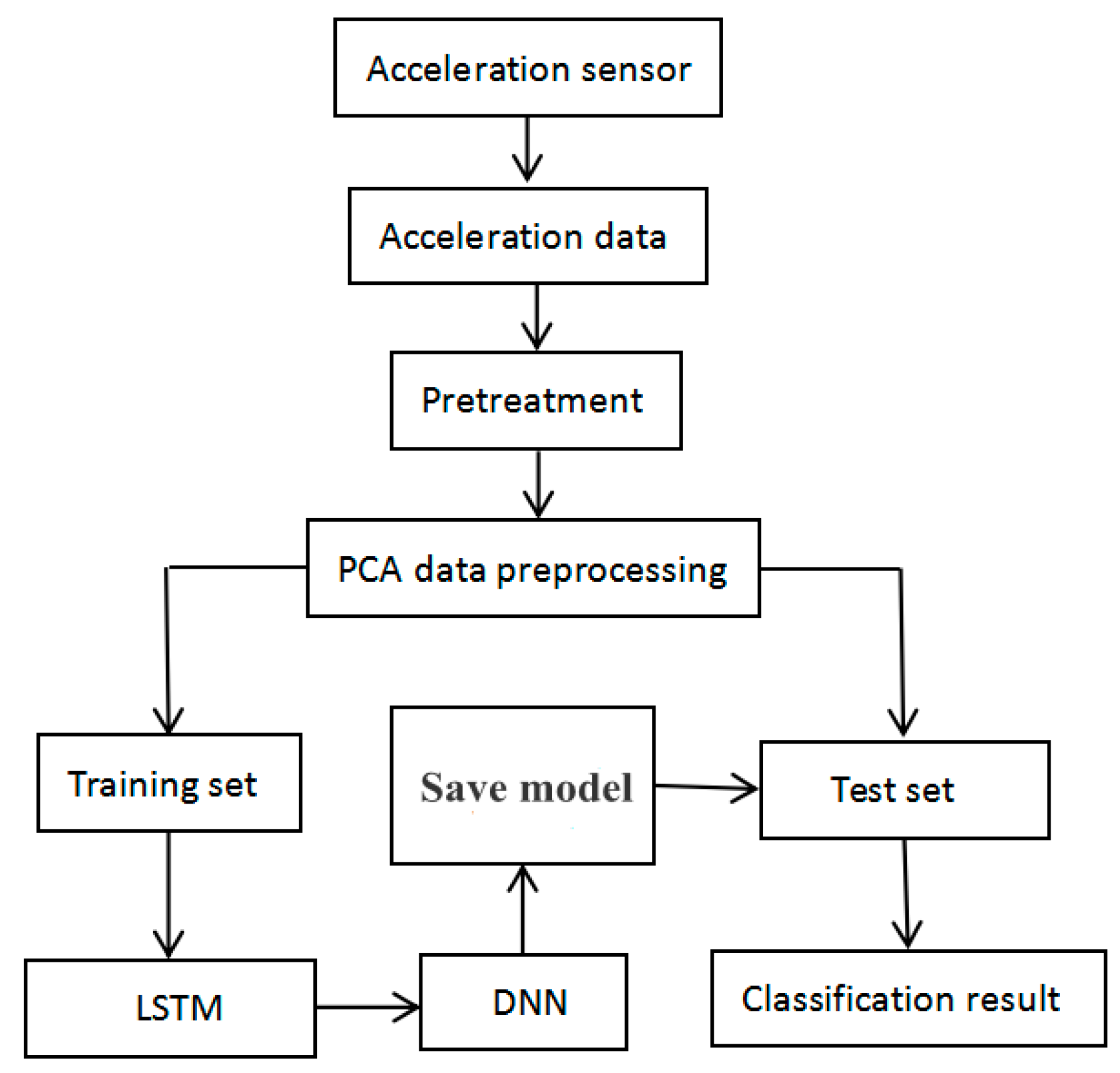
In this experiment, a total of more than 640,000 pieces of acceleration information were collected. To avoid overfitting, three of the data were used for training and the other was used for testing. In this study, we randomly selected data from three subjects to train the LSTM-DNN model and the other three models. Use the remaining data from one subject to verify the performance of the model. In addition, the final model parameters were determined after 15,000 network trainings. The overall process is shown in Figure 7.
3.5. Evaluation Methods
A single measure cannot be used to determine the performance of the algorithm and compare different methods. Commonly used methods to compare the performance of different approaches include precision, recall, accuracy, and F-score. Accuracy is defined as the ratio of the number of samples that are classified correctly to the total number of samples and its expression is shown in Equation (9). Precision and recall are two measures widely used in the fields of information retrieval and statistical classification to evaluate the quality of the results. Precision measures the precision of the retrieval system and recall measures the recall rate of a retrieval system, whose expressions are shown in Equations (10) and (11). It is expected that the higher the precision, the better the results are. The higher the recall, the better the results are. The F-score integrates the results of the precision and recall and its expression is shown in Equation (12); when the F-score is high, both precision and recall are high. The following equations [48,49] show the calculation of the evaluation factors, where TP, TN, FP, and FN represent true positive, true negative, false positive, and false negative, respectively.
4. Experimental Results
From Table 2, it can be found that the SVM model has the highest accuracy and F-score value when the RBF kernel function is taken at the step speed of 0.78 m/s, 1.0 m/s, and 1.25 m/s. Thus, it can be determined that the kernel function of the SVM is an RBF kernel function. When the kernel function of SVM selects RBF, the recognition accuracy of the model under three kinds of asynchronous speeds is 77%, 71%, and 75%, respectively, and the F-score value of the model also reaches 78%, 72.8% and 75.9%, respectively. From Table 3, it can be found that the KNN model has the highest accuracy and F-score value when the pace is 0.78 m/s and 1.0 m/s. When K takes 2, the accuracy and F-score value are the highest. Thus, it can be determined that the K value of the KNN is 5, 5, 2, respectively, at a step speed of 0.78 m/s, 1.0 m/s, and 1.25 m/s. KNN’s accuracy is 76%, 69%, and 73% at three different paces, and its F-score is 77%, 70%, and 75% at three different paces.
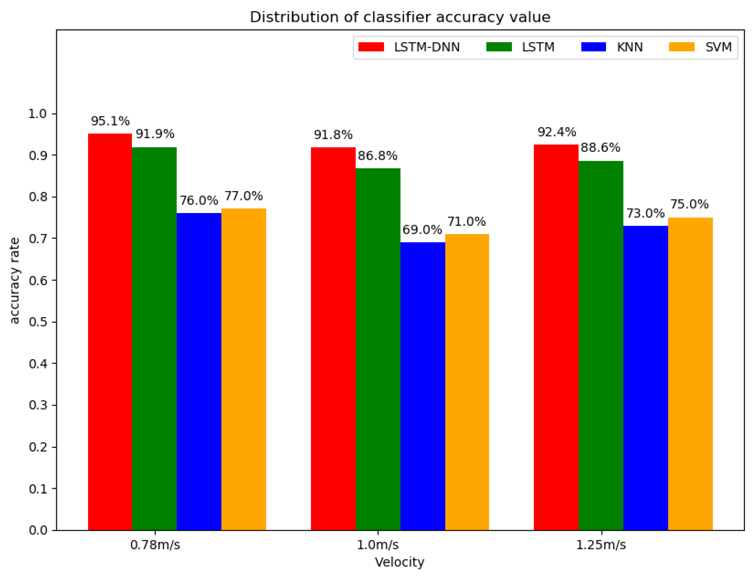
Table 4, Table 5, and Table 6 respectively classify the performance for each training function in terms of stance and swing phases under three kinds of sync speed. According to Table 4, Table 5, and Table 6, it can be observed that the LSTM-DNN algorithm has more than 91% and 92% gait phase accuracy and F-score at three different paces. In addition, we can see that LSTM-DNN and LSTM have a high recognition rate of gait phase, with both accuracy rates and F-scores over 86%. However, both KNN and SVM algorithms have a low recognition rate of gait phase, with accuracy and F-scores less than 86%.
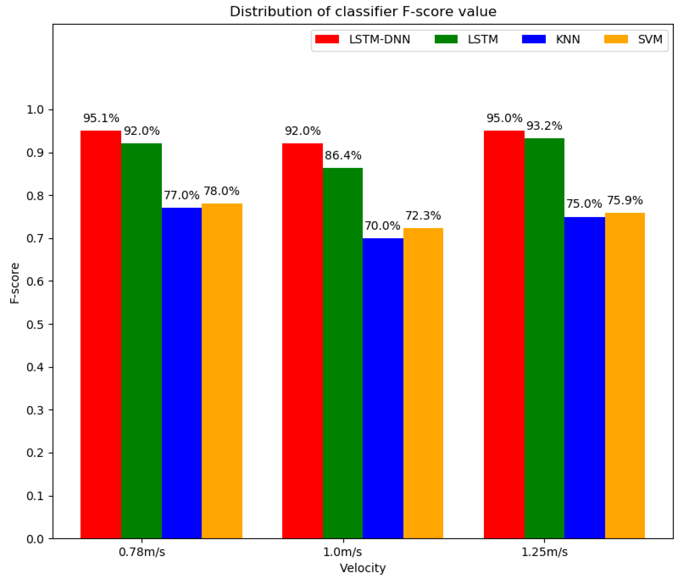
The recognition performance of LSTM-DNN, LSTM, SVM, and KNN algorithms for gait phase at three different walking speeds are shown in Figure 8 and Figure 9. It can be clearly seen from Figure 8 and Figure 9 that the LSTM-DNN algorithm is higher in accuracy and F-score than the other three algorithms at any of the paces. As aforementioned, F-score can comprehensively measure the two indicators of precision and recall. It was observed that the F-score of KNN and SVM are too low compared to the LSTM-DNN and LSTM and it can also be seen that the LSTM-DNN algorithm outperforms the other three algorithms in terms of accuracy and F-score, thus verifying the effectiveness of the LSTM-DNN algorithm.
5. Discussion
This study demonstrated the capability of the proposed system to detect gait phases based on acceleration signals. To support this hypothesis, this paper proposes to use the LSTM-DNN to identify the gait phase, and compares it with other algorithms to verify the effectiveness of the algorithm.
Walking activity emanated from the human body is important, and this information can be extracted through the use of acceleration signals. Although the LSTM-DNN algorithm has shown certain validity in the classification of acceleration signals for gait event detection, it still needs to be further optimized in the future. In this study, the inertial sensor module needed to be placed at a designated location on the instep, lower leg, and thigh of each subject. However, due to the height, weight, gender, etc., of each tester, the sensor cannot be accurately placed in the specified position and can only be installed at an approximate designated position, which needs further investigation.
To characterize acceleration signals, there are three main cascaded modules which are data-processing, feature extraction, and classification methods. Feature extraction is the crucial step. The research result in this study shows that the LSTM-DNN algorithm can accurately identify the phase through the five features selected in this paper. By observing Table 2 and Table 3, we can get that the kernel function has certain influence on the performance of SVM and the influence of the choice of K value on KNN is also very important. By analyzing the results of Table 4, Table 5 and Table 6, it can be shown that the SVM and KNN have low accuracy of the gait phase detection, but the proposed LSTM-DNN algorithm in this paper can significantly improve this situation.
In reviewing the literature, the reliability of the accelerometer was questioned. It is interesting to note that the speed sensor had to be worn in the designated position of each subject’s foot, calf, and thigh. However, due to the difference in the height, weight, and gender of the test subjects, there may be slight differences in the position of the sensor. According to Figure 8 and Figure 9, it can be found that the recognition accuracy and F-score from the LSTM-DNN algorithm have been as high as 91%, which indicates that the generalization performance of the LSTM-DNN algorithm is better, and it is less affected by factors such as gender, height, weight, and pace.
The purpose of this study was to apply machine learning to predict stance and swing phases from acceleration signals. In support of the hypothesis aforementioned, this study proposes the LSTM-DNN algorithm and uses it to successfully predict stance and swing phases. The results of learned data indicated that the acceleration signals had low variability and stability during walking on the ground. The LSTM-DNN algorithm fuses the LSTM model with the DNN model and uses 36 LSTM networks. In the experiment, we conducted a lot of experiments and found that when the number of LSTM units is 36, the recognition effect is better. In addition, it is difficult to achieve the desired effect by simply relying on a single LSTM network structure. By introducing the DNN structure, the unity of the network structure can be improved, and the recognition effect can be improved. Thus, the model used in this paper can achieve higher recognition accuracy, and the F-score value is higher than 92%. It can be seen from Table 4, Table 5 and Table 6 that the F-score of the LSTM-DNN algorithm is the largest, followed by the LSTM algorithm, and the F-score of the KNN algorithm is the smallest. It can be seen from the performance of each classifier in F-score that the classification result obtained by the LSTM-DNN algorithm is more reliable.
In terms of the generalization of the proposed system, this study revealed the LSTM-DNN algorithm achieved better performance in gait phase recognition. The LSTM-DNN algorithm detects stance and swing phases with higher recognition accuracy and F-score than other algorithms. From the SVM and KNN, the recognition of the phase is relatively poor; we can see that the proposed use of the five features to distinguish between stance and swing phases may still has certain drawbacks.
6. Conclusions
In this paper, a gait phase detection method based on the LSTM-DNN algorithm was presented. Compared with the commonly used LSTM, SVM, and KNN algorithms, the recognition accuracy and F-score of the LSTM-DNN algorithm for gait phase detection are as high as 91.8% and 92%, respectively, demonstrating the superiority of the LSTM-DNN algorithm. The experimental results showed that the LSTM-DNN algorithm was effective for distinguishing the two gait phases of the lower limb.
In this study, wearable acceleration devices were used to collect the acceleration data of the lower limb and the gait phase of test subjects was automatically detected and classified. Although the LSTM-DNN algorithm was effective for gait phase detection, further optimization of the model is required. Future studies will focus on improving the accuracy of the gait classification and investigating factors that may affect the gait. In this study, the use of three acceleration sensors was considered acceptable. However, the presence of the sensors may have a potential impact on people’s gait.
The LSTM-DNN algorithm is a promising approach to process acceleration signals for gait recognition at different walking speeds. In the future, the LSTM-DNN algorithm will be used to analyze more complex gait patterns and other applications will be investigated. Gait phase recognition technology plays an important role in the human–machine coupling of the human lower extremity exoskeleton assisting robot, and is of great significance to the development of the human lower extremity exoskeleton assisting robot. In addition, gait phase recognition technology has great potential in pathological gait recognition and diagnosis.
Author Contributions
Writing–review & editing, T.Z. and L.Y.; investigation, P.Y.; funding acquisition, L.Y.
Funding
This research was funded by the Fundamental Research Funds for the Central Universities (No. 2015ZCQ-GX-03).
Conflicts of Interest
The authors declare no conflict of interest.
References
- Wu, W.H.; Bui, A.A.; Batalin, M.A.; Liu, D.; Kaiser, W.J. Incremental diagnosis method for intelligent wearable sensor systems. IEEE Trans. Inf. Technol. Biomed. 2007, 11, 553–562. [Google Scholar] [CrossRef] [PubMed]
- Veneman, J.; Kruidhof, R.; Hekman, E.; Ekkelenkamp, R.; Van Asseldonk, E.; van der Kooij, H. Design and Evaluation of the LOPES Exoskeleton Robot for Interactive Gait Rehabilitation. IEEE Trans. Neural Syst. Rehabil. Eng. 2007, 15, 379–386. [Google Scholar] [CrossRef] [PubMed]
- Alexander, N.B.; Goldberg, A. Gait disorders: Search for multiple causes. Clevel. Clin. J. Med. 2005, 72, 586–594. [Google Scholar] [CrossRef] [PubMed]
- Okubo, Y.; Schoene, D.; Lord, S.R. Step training improves reaction time, gait and balance and reduces falls in older people: A systematic review and meta-analysis. Br. J. Sports Med. 2017, 51, 586–593. [Google Scholar] [CrossRef]
- Abellanas, A.; Frizera, A.; Ceres, R.; Gallego, J.A. Estimation of gait parameters by measuring upper limb-walker interaction forces. Sens. Actuators A Phys. 2010, 162, 276–283. [Google Scholar] [CrossRef]
- Figueiredo, J.; Ferreira, C.; Santos, C.P.; Moreno, J.C.; Reis, L.P. Real-Time Gait Events Detection during Walking of Biped Model and Humanoid Robot through Adaptive Thresholds. In Proceedings of the 2016 International Conference on Autonomous Robot Systems and Competitions (ICARSC), Bragança, Portugal, 4–6 May 2016; pp. 66–71. [Google Scholar]
- Vu, H.T.T.; Gomez, F.; Cherelle, P.; Lefeber, D.; Nowé, A.; Vanderborght, B. ED-FNN: A New Deep Learning Algorithm to Detect Percentage of the Gait Cycle for Powered Prostheses. Sensors 2018, 18, 2389. [Google Scholar] [CrossRef]
- Murray, S.; Goldfarb, M. Towards the use of a lower limb exoskeleton for locomotion assistance in individuals with neuromuscular locomotor deficits. In Proceedings of the 2012 Annual International Conference of the IEEE Engineering in Medicine and Biology Society, San Diego, CA, USA, 28 August–1 September 2012; Volume 2012, pp. 1912–1915. [Google Scholar]
- Yan, T.; Cempini, M.; Oddo, C.M.; Vitiello, N. Review of assistive strategies in powered lower-limb orthoses and exoskeletons. Robot. Auton. Syst. 2015, 64, 120–136. [Google Scholar] [CrossRef]
- Juri, T.; Eduardo, P.; Stefano, R.; Cappa, P. Gait Partitioning Methods: A Systematic Review. Sensors 2016, 16, 66. [Google Scholar]
- Taborri, J.; Scalona, E.; Rossi, S.; Palermo, E.; Patane, F.; Cappa, P. Real-time gait detection based on Hidden Markov Model: Is it possible to avoid training procedure? In Proceedings of the 2015 IEEE International Symposium on Medical Measurements and Applications (MeMeA), Torino, Italy, 7–9 May 2015; pp. 141–145. [Google Scholar]
- González, I.; Fontecha, J.; Hervás, R.; Bravo, J. An Ambulatory System for Gait Monitoring Based on Wireless Sensorized Insoles. Sensors 2015, 15, 16589–16613. [Google Scholar] [CrossRef]
- Anwary, A.R.; Yu, H.; Vassallo, M. Optimal foot location for placing wearable IMU sensors and automatic feature extraction for gait analysis. IEEE Sens. J. 2018, 18, 2555–2567. [Google Scholar] [CrossRef]
- Rosati, S.; Agostini, V.; Knaflitz, M.; Balestra, G. Muscle activation patterns during gait: A hierarchical clustering analysis. Biomed. Signal Process. Control 2017, 31, 1746–8094. [Google Scholar] [CrossRef]
- Goršič, M.; Kamnik, R.; Ambrožič, L.; Vitiello, N.; Lefeber, D.; Pasquini, G.; Munih, M. Online phase detection using wearable sensors for walking with a robotic prosthesis. Sensors 2014, 14, 2776–2794. [Google Scholar] [CrossRef] [PubMed]
- Yang, G.; Tan, W.; Jin, H.; Zhao, T.; Tu, L. Review wearable sensing system for gait recognition. Cluster Comput. 2018, 22, 3021–3029. [Google Scholar] [CrossRef]
- Yuwono, M.; Su, S.W.; Guo, Y.; Moulton, B.D.; Nguyen, H.T. Unsupervised nonparametric method for gait analysis using a waist-worn inertial sensor. Appl. Soft Comput. J. 2014, 14, 72–80. [Google Scholar] [CrossRef]
- Guenterberg, E.; Yang, A.Y.; Ghasemzadeh, H.; Jafari, R.; Bajcsy, R.; Sastry, S.S. A Method for Extracting Temporal Parameters Based on Hidden Markov Models in Body Sensor Networks With Inertial Sensors. IEEE Trans. Inf. Technol. Biomed. 2009, 13, 1019–1030. [Google Scholar] [CrossRef]
- Shimada, Y.; Ando, S.; Matsunaga, T.; Misawa, A.; Aizawa, T.; Shirahata, T.; Itoi, E. Clinical application of acceleration sensor to detect the swing phase of stroke gait in functional electrical stimulation. Tohoku J. Exp. Med. 2005, 207, 197. [Google Scholar] [CrossRef]
- Taborri, J.; Rossi, S.; Palermo, E.; Patanè, F.; Cappa, P. A Novel HMM Distributed Classifier for the Detection of Gait Phases by Means of a Wearable Inertial Sensor Network. Sensors 2014, 14, 16212–16234. [Google Scholar] [CrossRef]
- Kim, M.; Lee, D. Development of an IMU-based foot-ground contact detection (FGCD) algorithm. Ergonomics 2017, 60, 384–403. [Google Scholar] [CrossRef]
- Mukherjee, J.; Chattopadhyay, P.; Sural, S. Information fusion from multiple cameras for gait-based re-identification and recognition. IET Image Process. 2015, 9, 969–976. [Google Scholar]
- Ding, S.; Ouyang, X.; Li, Z.; Yang, H. Proportion-Based Fuzzy Gait Phase Detection Using the Smart Insole. Sens. Actuators A Phys. 2018, 284, 96–102. [Google Scholar] [CrossRef]
- Wang, Z.; Shibai, K.; Kiryu, T. An Internet-based cycle ergometer system by using distributed computing. In Proceedings of the 4th International IEEE EMBS Special Topic Conference on Information Technology Applications in Biomedicine, 2003, Birmingham, UK, 24–26 April 2003. [Google Scholar]
- Bejarano, N.C.; Ambrosini, E.; Pedrocchi, A.; Ferrigno, G.; Monticone, M.; Ferrante, S. A Novel Adaptive, Real-Time Algorithm to Detect Gait Events From Wearable Sensors. IEEE Trans. Neural Syst. Rehabil. Eng. 2015, 23, 413–422. [Google Scholar] [CrossRef] [PubMed]
- Caldas, R.; Mundt, M.; Potthast, W.; de Lima Neto, F.B.; Markert, B. A systematic review of gait analysis methods based on inertial sensors and adaptive algorithms. Gait Posture 2017, 57, 204–210. [Google Scholar] [CrossRef] [PubMed]
- Sánchez Manchola, M.D.; Bernal MJ, P.; Munera, M.; Cifuentes, C.A. Gait Phase Detection for Lower-Limb Exoskeletons using Foot Motion Data from a Single Inertial Measurement Unit in Hemiparetic Individuals. Sensors 2019, 19, 2988. [Google Scholar] [CrossRef] [PubMed]
- Kavanagh, J.J.; Menz, H.B. Accelerometry: A technique for quantifying movement patterns during walking. Gait Posture 2008, 28, 1–15. [Google Scholar] [CrossRef] [PubMed]
- McCamley, J.; Donati, M.; Grimpampi, E.; Mazza, C. An enhanced estimate of initial contact and final contact instants of time using lower trunk inertial sensor data. Gait Posture 2012, 36, 316–318. [Google Scholar] [CrossRef] [PubMed]
- Ma, S.Q. Research on improved pca-lda face recognition algorithm. J. Shaanxi Univ. Sci. Technol. (Nat. Sci. Ed.) 2019, 62–66. [Google Scholar]
- Parente, A.; Sutherland, J.C. PCA and Kriging for the efficient exploration of consistency regions in Uncertainty Quantification. Combust. Flame 2013, 160, 340–350. [Google Scholar] [CrossRef]
- Coussement, A.; Isaac, B.J.; Gicquel, O.; Parente, A. Assessment of different chemistry reduction methods based on principal component analysis: Comparison of the MG-PCA and score-PCA approaches. Combust. Flame 2016, 168, 83–97. [Google Scholar] [CrossRef]
- Lu, X.L.; Xu, X. Human behavior recognition based on acceleration and hga-bp neural network. Comput. Eng. 2015, 41, 220–224, 232. [Google Scholar]
- Rueterbories, J.; Spaich, E.G.; Andersen, O.K. Gait event detection for use in FES rehabilitation by radialand tangential foot accelerations. Med. Eng. Phys. 2014, 36, 502–508. [Google Scholar] [CrossRef]
- Mummolo, C.; Mangialardi, L.; Kim, J.H. Quantifying dynamic characteristics of human walking for comprehensive gait cycle. J. Biomech. Eng. 2013, 135, 91006. [Google Scholar] [CrossRef] [PubMed]
- Su, X.; Tong, H.; Ji, P. Activity recognition with smartphone sensors. J. Tsinghua Univ. (Nat. Sci. Ed.) 2014, 19, 235–249. [Google Scholar]
- Mileti, I.; Germanotta, M.; Di Sipio, E.; Imbimbo, I.; Pacilli, A.; Erra, C.; Petracca, M.; Rossi, S.; Del Prete, Z.; Bentivoglio, A.R.; et al. Measuring Gait Quality in Parkinson’s Disease through Real-Time Gait Phase Recognition. Sensors 2018, 18, 919. [Google Scholar] [CrossRef] [PubMed]
- Dong, G. Research on Human Behavior Recognition Technology Based on Multi-Feature Fusion. Master’s Thesis, Tianjin University of Technology, Tianjin, China, 2017. [Google Scholar]
- Daud, W.M.B.W.; Yahya, A.B.; Horng, C.S.; Sulaima, M.F.; Sudirman, R. Features extraction of electromyography signals in time domain on biceps brachii muscle. Int. J. Model. Optim. 2013, 3, 515–519. [Google Scholar] [CrossRef]
- Hochreiter, S.; Schmidhuber, J. Long Short-Term Memory. Neural Comput. 1997, 9, 1735–1780. [Google Scholar] [CrossRef]
- Donahue, J.; Anne Hendricks, L.; Guadarrama, S.; Rohrbach, M.; Venugopalan, S.; Saenko, K.; Darrell, T. Long-term recurrent convolutional networks for visual recognition and description. IEEE Trans. Pattern Anal. Mach. Intell. 2017, 39, 677–691. [Google Scholar] [CrossRef]
- Bai, Y.; Jin, X.; Wang, X.; Su, T.; Kong, J.; Lu, Y. Compound Autoregressive Network for Prediction of Multivariate Time Series. Complexity 2019, 2019, 9107167. [Google Scholar] [CrossRef]
- Bai, Y.T.; Wang, X.Y.; Sun, Q.; Jin, X.B.; Wang, X.K.; Su, T.L.; Kong, J.L. Spatio-Temporal Prediction for the Monitoring-Blind Area of Industrial Atmosphere Based on the Fusion Network. Int. J. Environ. Res. Public Health 2019, 16, 3788. [Google Scholar] [CrossRef] [Green Version]
- Jin, X.B.; Yang, N.; Wang, X.; Bai, Y.; Su, T.; Kong, J. Integrated predictor based on decomposition mechanism for PM2.5 long-term prediction. Appl. Sci. Basel 2019, 9, 4533. [Google Scholar] [CrossRef] [Green Version]
- Shahrebabaki, A.S.; Imran, A.S.; Olfati, N.; Svendsen, T. A Comparative Study of Deep Learning Techniques on Frame-Level Speech Data Classification. Circuits Syst. Signal Process. 2019, 38, 3501–3520. [Google Scholar] [CrossRef]
- Wang, X.; Tang, M.; Yang, S.; Yin, H.; Huang, H.; He, L. Automatic Hypernasality Detection in Cleft Palate Speech Using CNN. Circuits Syst. Signal Process. 2019, 38, 3521–3547. [Google Scholar] [CrossRef]
- Wang, C.; Li, K. Aitken-Based Stochastic Gradient Algorithm for ARX Models with Time Delay. Circuits Syst. Signal Process. 2018, 38, 2863–2876. [Google Scholar] [CrossRef]
- Zheng, Y.Y.; Kong, J.L.; Jin, X.B.; Wang, X.Y.; Su, T.L.; Wang, J.L. Probability Fusion Decision Framework of Multiple Deep Neural Networks for Fine-Grained Visual Classification. IEEE Access 2019, 7, 122740–122757. [Google Scholar] [CrossRef]
- Zheng, Y.Y.; Kong, J.L.; Jin, X.B.; Wang, X.Y.; Su, T.L.; Zuo, M. CropDeep: The Crop Vision Dataset for Deep-Learning-Based Classification and Detection in Precision Agriculture. Sensors 2019, 19, 1058. [Google Scholar] [CrossRef] [Green Version]
Figure 1.
Human lower limb movement and gait information acquisition system.

Figure 2.
Acceleration data collected under the three body parts: foot (a), calf (b), and thigh (c). a_x represents the acceleration in the x-axis direction, a_y represents the acceleration in the y-axis direction, a_z represents the acceleration in the z-axis direction, a_com represents the combined acceleration.

Figure 3.
Schematic diagram of the gait phase division. a_x represents the acceleration in the x-axis direction, a_y represents the acceleration in the y-axis direction, a_z represents the acceleration in the z-axis direction.
Figure 3.
Schematic diagram of the gait phase division. a_x represents the acceleration in the x-axis direction, a_y represents the acceleration in the y-axis direction, a_z represents the acceleration in the z-axis direction.

Figure 4.
Sliding window segmentation of acceleration data. Here RF represents the acquired foot acceleration data, RC represents the acquired calf acceleration data, and RT represents the collected thigh acceleration data.
Figure 4.
Sliding window segmentation of acceleration data. Here RF represents the acquired foot acceleration data, RC represents the acquired calf acceleration data, and RT represents the collected thigh acceleration data.

Figure 5.
Long short-term memory (LSTM) cell structure.

Figure 6.
Schematic diagram of the LSTM-DNN structure.

Figure 7.
Flow chart of the analysis process.

Figure 8.
Distribution of accuracy values of four classifiers.

Figure 9.
Distribution of F-score values of four classifiers.


Table 1.
Acceleration data for different parts at different speeds using a principal components analysis (PCA) synthesized parameter table.
Table 1.
Acceleration data for different parts at different speeds using a principal components analysis (PCA) synthesized parameter table.
| Pace | Collection Location | z_1 | z_2 | z_3 |
|---|---|---|---|---|
| 0.78 m/s | Calf | 0.658 | 0.659 | 0.365 |
| Thigh | −0.556 | 0.569 | 0.365 | |
| Foot | 0.645 | 0.499 | 0.579 | |
| 1.0 m/s | Calf | 0.636 | 0.645 | 0.423 |
| Thigh | −0.479 | 0.597 | 0.643 | |
| Foot | 0.667 | 0.545 | 0.508 | |
| 1.25 m/s | Calf | 0.639 | 0.631 | 0.440 |
| Thigh | −0.565 | 0.533 | 0.630 | |
| Foot | 0.703 | 0.566 | 0.431 |
Table 2.
Performance of SVM algorithm under different parameters.
| Kernel Function | Pace | Accuracy | Precision | Recall | F-score |
|---|---|---|---|---|---|
| Linear | 0.78 m/s | 0.590 | 0.680 | 0.600 | 0.638 |
| 1.00 m/s | 0.660 | 0.710 | 0.670 | 0.689 | |
| 1.25 m/s | 0.720 | 0.720 | 0.710 | 0.715 | |
| rbf | 0.78 m/s | 0.770 | 0.780 | 0.780 | 0.780 |
| 1.00 m/s | 0.710 | 0.770 | 0.690 | 0.728 | |
| 1.25 m/s | 0.750 | 0.780 | 0.740 | 0.759 | |
| poly | 0.78 m/s | 0.490 | 0.250 | 0.500 | 0.333 |
| 1.00 m/s | 0.500 | 0.250 | 0.500 | 0.333 | |
| 1.25 m/s | 0.610 | 0.610 | 0.610 | 0.610 | |
| sigmoid | 0.78 m/s | 0.500 | 0.250 | 0.500 | 0.333 |
| 1.00 m/s | 0.610 | 0.640 | 0.600 | 0.650 | |
| 1.25 m/s | 0.630 | 0.630 | 0.630 | 0.630 |
Table 3.
Performance of k-nearest neighbor method (KNN) algorithm under different parameters.
| K | Pace | Accuracy | Precision | Recall | F-score |
|---|---|---|---|---|---|
| 2 | 0.78 m/s | 0.690 | 0.740 | 0.670 | 0.703 |
| 1.00 m/s | 0.620 | 0.700 | 0.630 | 0.663 | |
| 1.25 m/s | 0.730 | 0.760 | 0.740 | 0.750 | |
| 5 | 0.78 m/s | 0.760 | 0.780 | 0.760 | 0.770 |
| 1.00 m/s | 0.690 | 0.700 | 0.700 | 0.700 | |
| 1.25 m/s | 0.720 | 0.730 | 0.730 | 0.730 | |
| 7 | 0.78 m/s | 0.700 | 0.740 | 0.700 | 0.719 |
| 1.00 m/s | 0.680 | 0.710 | 0.680 | 0.695 | |
| 1.25 m/s | 0.640 | 0.660 | 0.630 | 0.645 | |
| 10 | 0.78 m/s | 0.670 | 0.730 | 0.660 | 0.693 |
| 1.00 m/s | 0.650 | 0.660 | 0.640 | 0.619 | |
| 1.25 m/s | 0.680 | 0.690 | 0.680 | 0.685 | |
| 15 | 0.78 m/s | 0.670 | 0.690 | 0.670 | 0.680 |
| 1.00 m/s | 0.670 | 0.680 | 0.670 | 0.675 | |
| 1.25 m/s | 0.570 | 0.690 | 0.620 | 0.653 | |
| 20 | 0.78 m/s | 0.640 | 0.680 | 0.620 | 0.649 |
| 1.00 m/s | 0.600 | 0.620 | 0.590 | 0.605 | |
| 1.25 m/s | 0.620 | 0.650 | 0.630 | 0.640 | |
| 30 | 0.78 m/s | 0.610 | 0.670 | 0.610 | 0.639 |
| 1.00 m/s | 0.620 | 0.660 | 0.630 | 0.645 | |
| 1.25 m/s | 0.520 | 0.550 | 0.510 | 0.529 |
Table 4.
Performance of different algorithms for a walking speed of 0.78 m/s.
| Algorithm | Accuracy | Precision | Recall | F-score |
|---|---|---|---|---|
| LSTM-DNN | 0.951 | 0.962 | 0.941 | 0.951 |
| LSTM | 0.919 | 0.939 | 0.901 | 0.920 |
| KNN | 0.760 | 0.780 | 0.760 | 0.770 |
| SVM | 0.770 | 0.780 | 0.780 | 0.780 |
Table 5.
Performance of different algorithms for a walking speed of 1.0 m/s.
| Algorithm | Accuracy | Precision | Recall | F-score |
|---|---|---|---|---|
| LSTM-DNN | 0.918 | 0.936 | 0.905 | 0.920 |
| LSTM | 0.868 | 0.903 | 0.828 | 0.864 |
| KNN | 0.690 | 0.700 | 0.700 | 0.700 |
| SVM | 0.710 | 0.770 | 0.690 | 0.728 |
Table 6.
Performance of different algorithms for a walking speed of 1.25 m/s.
| Algorithm | Accuracy | Precision | Recall | F-score |
|---|---|---|---|---|
| LSTM-DNN | 0.924 | 0.913 | 0.946 | 0.950 |
| LSTM | 0.886 | 0.891 | 0.881 | 0.932 |
| KNN | 0.730 | 0.760 | 0.740 | 0.750 |
| SVM | 0.750 | 0.780 | 0.740 | 0.759 |
© 2019 by the authors. Licensee MDPI, Basel, Switzerland. This article is an open access article distributed under the terms and conditions of the Creative Commons Attribution (CC BY) license (http://creativecommons.org/licenses/by/4.0/).
Share and Cite
MDPI and ACS Style
Zhen, T.; Yan, L.; Yuan, P. Walking Gait Phase Detection Based on Acceleration Signals Using LSTM-DNN Algorithm. Algorithms 2019, 12, 253. https://0-doi-org.brum.beds.ac.uk/10.3390/a12120253
AMA Style
Zhen T, Yan L, Yuan P. Walking Gait Phase Detection Based on Acceleration Signals Using LSTM-DNN Algorithm. Algorithms. 2019; 12(12):253. https://0-doi-org.brum.beds.ac.uk/10.3390/a12120253
Chicago/Turabian StyleZhen, Tao, Lei Yan, and Peng Yuan. 2019. "Walking Gait Phase Detection Based on Acceleration Signals Using LSTM-DNN Algorithm" Algorithms 12, no. 12: 253. https://0-doi-org.brum.beds.ac.uk/10.3390/a12120253
Note that from the first issue of 2016, this journal uses article numbers instead of page numbers. See further details here.