Graph Theory Approach to the Vulnerability of Transportation Networks

Abstract

Nowadays, transport is the basis for the functioning of national, continental, and global economies. Thus, many governments recognize it as a critical element in ensuring the daily existence of societies in their countries. Those responsible for the proper operation of the transport sector must have the right tools to model, analyze, and optimize its elements. One of the most critical problems is the need to prevent bottlenecks in transport networks. Thus, the main aim of the article was to define the parameters characterizing the transportation network vulnerability and select algorithms to support their search. The parameters proposed are based on characteristics related to domination in graph theory. The domination, edge-domination concepts, and related topics, such as bondage-connected and weighted bondage-connected numbers, were applied as the tools for searching and identifying the bottlenecks in transportation networks. Furthermore, the algorithms for finding the minimal dominating set and minimal (maximal) weighted dominating sets are proposed. This way, the exemplary academic transportation network was analyzed in two cases: stationary and dynamic. Some conclusions are presented. The main one is the fact that the methods given in this article are universal and applicable to both small and large-scale networks. Moreover, the approach can support the dynamic analysis of bottlenecks in transport networks.

1. Introduction

Globalization forces every business activity to be flexible and free of weaknesses. One of the critical branches is transport, which, together with:

• Energy;
• Information and communication technology;
• Agriculture (water, food);
• Finance, public and legal order, and safety;

Constitute the foundations of the activity of societies in developing and developed countries. Not without reason, among others, these branches are recognized by individual countries as critical systems or critical infrastructures [1,2,3,4,5]. Therefore, addressing the vulnerability of transport networks is the key to reliable operation of transport and logistics systems [6,7,8]. This is particularly important in the context of climate change [9,10,11,12,13] and the need to preserve the business continuity of these networks [9,12,14]. It was assumed that the best and most natural way to describe transport systems was a graph network representing the infrastructure of this system and allowing characterization of the traffic flows occurring in this network [15,16,17,18]. One should agree with this because the structure and traffic flow in the transport network reflect the relationships between individual elements of the transport system in the best way, and thus, determine it [8,12]. According to the above, one of the most important things in transportation networks’ analysis is the finding of the bottlenecks. They impose delays and restrictions in the normal flow of transportation [18,19,20,21,22]. There are three major types of bottlenecks:

• Infrastructure bottlenecks—can be the outcome of chronic or temporary conditions (e.g., factors: climate change, traffic expansions, such as a bridge or a port).
• Regulations bottlenecks—can be the results of regulations that delay goods movement for security or safety inspections (in international transport: custom procedures for passengers and freight).
• Supply chain bottlenecks—can be results of specific tasks and procedures in supply chain management (labor availability—work shifts may impose time-dependent capacity shortages; some firms may create bottlenecks on purpose as a rent-seeking strategy since they control key elements of the supply chain; different information exchange protocols can create delays in information processing, and therefore, delays in shipments).

The article provides parameters characterizing the transport network’s vulnerability and algorithms for their determination. The proposed tools were based on the graph theory concepts, particularly domination topics [23,24,25]. It should be mentioned that the use of the domination in graphs allows one to:

• Minimize the distance to the critical points for the citizens under a fixed number of them;
• Reduce the number of base stations needed to support all of its users;
• Select the minimum number of representatives necessary for the overall monitoring of communication networks.

2. Materials and Methods

2.1. General Assumptions

In this paper, we consider the connected, simple, undirected graph $G=(V,E)$, where V is the set of vertices (nodes), and  E is the set of edges (arcs). Sometimes, we use the fuller notation for graph G, where $V\left(G\right)$ and $E\left(G\right)$ denote its vertex-set and the edge-set respectively. The assumption about connectivity is important, because it is fundamental to the functioning of transport or logistics networks. Some basic definitions of graph theory are necessary to understand ways of the description of network graphs. The set of all adjacent vertices to vertex $v\in V$ in G is called neighborhood and denoted by $N_G\left(v\right)$ or $N\left(v\right)$. The close neighborhood of this vertex is defined as $N_G\left(v\right)\cup \left\{v\right\}$ and denoted by $N_G\left[v\right]$ or $N\left[v\right]$. The other basic parameter for graphs is the degree of vertex $v\in V$, which is defined as the number of vertices in $N_G\left(v\right)$ and denoted by $deg\left(v\right)$. The minimum and maximum degree are defined as $\delta \left(G\right)=min\{x\in V:deg(x\left)\right\}$ and $\Delta \left(G\right)=max\{x\in V:deg(x\left)\right\}$, respectively. Moreover, the set of all edges, incident to the vertex $v\in V$, is denoted by $I_G\left(v\right)$. For any set $A\subseteq F$, neighborhood is given by $N\left(A\right)={\bigcup }_{v\in A}N\left(v\right)$. The induced subgraph defined on A is denoted by $G\left[A\right]$.

Regarding the assumption about connectivity in graphs, it is said that two vertices u and v in graph G are called connected if G contains a path from u to v. Otherwise, they are called disconnected. A graph is said to be connected if every pair of vertices in the graph is connected. If the graph is disconnected, there is a connected component, which are maximal connected subgraphs of G. Each vertex belongs to exactly one connected component, as does each edge.

2.2. Current Indicators for Transportation Network Description

Kansky proposed in the 1960s [20,26]—through using graph theory to describe transport networks—several indicators describing transport networks with two levels of detail. The first one is related to determining parameters or indicators about the whole network, and the others concerning the nodes. The main objective of their applicability is that they provide methods to [20]:

• Express of the relationship between the values of these parameters and the structure of the network;
• Comparing the different transportation networks at certain points in time;
• Comparing the development of transport networks at different times.

According to the above, the well-known graph theory parameters describing the transportation networks are as follows [20,26]:

• Network level:
  • Cost, which represents the total length of the network measured in real transport distances.
  • Detour index is a measure of the efficiency of a transport network in terms of how well it overcomes distance or the friction of distance.
  • Network density measures the territorial occupation of a transport network in terms of km of links per square kilometers of surface.
  • Pi index describes the relationship between the total length of the graph and the distance along its diameter.
  • Eta index describes average length per link.
  • Theta Index measures the function of a node, which is the average amount of traffic per intersection.
  • Alpha index is a measure of connectivity which evaluates the number of cycles in a graph in comparison with the maximum number of cycles.
  • Beta index is a measure of the level of connectivity in a graph and is expressed by the relationship between the number of links e over the number of nodes v.
  • Gamma index is a measure of connectivity that considers the relationship between the number of observed links and the number of possible links.
• Node level:
  • Order (degree) of a node (o). The number of its attached links; it is a simple, but effective measure of nodal importance.
  • Koenig number (or associated number, eccentricity) is a measure of fairness based on the number of links needed to reach the most distant node in the graph.
  • Hub dependence is a measure of node vulnerability that is the share of the highest traffic link in total traffic (weighted degree).
  • Average nearest neighbors degree is a measure of neighborhoods indicating the type of environment in which the node situates.
  • Cohesion index (ci) for a given edge $\{u,v\}$: this index measures the ratio between the number of common neighbors connected to nodes u and v and the total number of their neighbors.
  • Within-module degree (z-score) describes how well connected a node is to other nodes in the same module (or cluster, community).
  • The participation coefficient allows one to compare the number of links (order, degree) of node u to nodes in all clusters with its number of links within its own cluster.
  • Shimbel index (or Shimbel distance, nodal accessibility, nodality) is a measure of accessibility representing the sum of the length of all shortest paths connecting all other nodes in the graph.
  • Betweenness centrality (or shortest-path betweenness) is a measure of accessibility that is the number of times a node is crossed by shortest paths in the graph.

2.3. Selected Domination Concepts in Graph Theory

The domination theory in graphs has various applications, where the analysis of the communications network is one of most discussed in the literature [27,28,29,30,31,32,33]. Hence, the idea to apply the selected methods or parameters to the transportation network research field. One of these parameters is the dominating set and domination number. According to results given in [27] a set $D\subseteq V\left(G\right)$ is a dominating set of graph G, if for any $v\in V\left(G\right)$ either $v\in D$ or $N_G\left(v\right)\cap D=⌀$. While the minimum cardinality of a dominating set of graphs G is called a domination number of G and denoted as $\gamma \left(G\right)$. The above definitions refer to the general terms of undirected graphs. There are concepts related to weight functions, which allows one to define the vertex-weighted and edge-weighted graphs [23,27,30]. Generally, a vertex-weighted graph $(G,w_v)$ is defined as a graph G together with a positive weight-function on its vertex set $w_v:V\left(G\right)\to \mathrm{R}>0$. Similarly, an edge-weighted graph $(G,w_e)$ is defined as a graph G together with a positive weight-function on its edge set $w_e:E\left(G\right)\to \mathrm{R}>0$. These definitions are needed to define different types of weighted domination numbers in an undirected graph. Two of them are as follows [30]:

• The weighted domination number ${\gamma }_w$ of $(G,w_v)$ is the minimum weight $w\left(D\right)={\sum }_{v\in D}w\left(v\right)$ of a set $D\subseteq V\left(G\right)$ such that every vertex $v\in V$ is in D or has a neighbor in D;
• The weighted independent domination number of ${\gamma }_{I_w}$ of $(G,w_v)$ is the minimum weight $w\left(D_I\right)={\sum }_{v\in D_I}w\left(v\right)$ of a set $D_I\subseteq V\left(G\right)$ such that no two vertices of $D_I$ are connected by any edge of $(G,w)$.

Similarly, it can be done for directed graphs.

Taking into account the complexity of the minimum dominating set, we should state, that in general it is an NP-hard problem. Efficient approximation algorithms work out under the assumption that any dominating set problem can be formulated as a set covering problem. Thus, the greedy algorithm for finding dominating set is an analog of one that has been presented in [30,34]. The Algorithm 1 is formulated as follows [30,34].

Algorithm 1 Dominating-set-1.

1: Input$G=(V,E)$; 2: Output Dominating set of graph G; 3: Let $V=1,...,m$ and $D=\varphi$ define; 4: Greedy adds a new node to D in each iteration, until D forms a dominating set; 5: A node j, is said to be covered if $j\in D$ or if any neighbor of j is in D. A node that is not covered is said to be uncovered; 6: In each iteration, put into D the least indexed node that covers the maximum number of uncovered nodes; 7: Stop when all the nodes are covered.

The concept of the above algorithm is based on the greedy addition of vertices with the largest number of uncovered neighbors. And the Algorithm 2 is as follows [30,34].

Algorithm 2 Dominating-set-2.

1: Input$G=(V,E)$; 2: Output Dominating set of graph G; 3: Let $S:=0$; all vertices are white; 4: while (white vertices exist) do 5:  Select $v\in \left\{x\right|w\left(x\right)={max}_{u\in V}\left\{w\right(u\left)\right\}\}$; 6:  $S:=S\cup \left\{v\right\}$; vertices in S get black color and their neighbors get the gray color; 7: end while.

The above algorithm, like Algorithm 1, greedily selects white vertices and colors them in black and their neighbors in gray. In the case of the minimum connected dominating set, the greedy algorithm is also used. However, to define them some preliminaries are necessary [30,35].

Additionally, the concepts of edge-dominating set and edge-domination numbers constitute a significant part of research on domination in graphs. According to [27,28,33,34,36], these terms are defined in the following way. The set $X\subseteq E\left(G\right)$ is called the edge-dominating set of graph G, if every edge not in X has a neighbor in set X. The cardinality of a minimum edge-dominating set is called the edge-domination number of a graph G and is denoted by ${\gamma }^{\prime }\left(G\right)$. Furthermore, the weighted edge-domination number extends the possibility of their application to searching for the critical edge sets in graphs represented a transportation network. The weighted edge-domination number ${{\gamma }^{\prime }}_w\left(G\right)$ of edge-weighted graph $(G,w_e)$ is defined as the smallest weight $w\left(X\right)={\sum }_{e\in X}{w}_e\left(e\right)$ of all edges in edge-dominating set $X\subseteq E\left(G\right)$ [36].

Another interesting concept is introduced by Fink et al. in [37]. They examined a question concerning the vulnerability of the communications network under link failure. They supposed a situation where someone does not know which nodes in the network act as transmitters but does know that the set of such nodes can be built as a minimum dominating set in the related graph. Thus, they asked about the fewest number of communication links that he must serve so that at least one additional transmitter would be required so that communication with all sites is possible. In this way, they introduced the new parameter called the bondage number of a graph. It is defined in the following way. The bondage number of nonempty graph G is the minimum cardinality among all sets of edges E for which $\gamma (G-E)>\gamma \left(G\right)$ [37,38]. Thus, the bondage number of graph G describes the smallest number of edges whose removal from G leads to a graph with a domination number larger than that of G.

Because the above definition of bondage number is not enough for transportation network analysis, in [31], the author defined the bondage-connected number $b_c\left(G\right)$ of nonempty graph G. It means the minimum cardinality among all sets of edges E for which $\gamma (G-E)>\gamma \left(G\right)$ and graph $G-E$ is connected.

Finally, one more concept refers to the domination in graphs, so-called edge subdivision. This operation is defined as follows [28,29,30,32,39]. For a graph $G=(V,E)$, subdivision of the edge $e=uv\in E$ with vertex x leads to a graph with vertex set $V\cup \left\{x\right\}$ and edge set $\left(E\right\{uv\left\}\right)\cup \{ux,xv\}$. Let $G_{e,t}$ denote a graph obtained from G by subdivision of the edge e with t vertices (instead of edge $e=uv$ we put a path $(u,x_1,x_2,...,x_t,v)$). For $t=1$ we write $G_e$. This approach corresponds with the domination subdivision number $\xi \left(G\right)$ or $sd\left(G\right)$ of a graph G. It is the minimum number of edges that must be subdivided (where each edge can be subdivided at most once) to increase the domination number.

2.4. Basic Concepts of Vulnerability in Transport

The term vulnerablity is defined as a physical feature or operational attribute that makes an individual open to using or vulnerable to a given threat [40,41,42,43,44,45,46,47,48,49,50,51]. However, in terms of reliability, it can be measured as the probability that the system can be in a critical state or worse in less time than expected. This can be determined by certain external factors that cause large adverse effects on other sensitive systems (consequences above a fixed level). In other words, this approach can be expressed as the inherent properties of the system or part of its assets, community, and environment that make them vulnerable to the harmful effects of natural and anthropogenic threats. In the literature in the field of transport [41,42,43,44,45,46,47,48,49,50,51], the concept of vulnerability is used to describe the consequences for travel in the transport system or transportation network, which may extend the travel time, alter the length of the road, or limit the availability of services. In the case of transport networks or transport systems in general, the restriction of access to services may be due to natural disasters or harmful human activities. When we consider the transportation network as a complex system, it is possible to use the methods for characterizing the vulnerability of this type of system. One way is to use topological indices derived from the algebraic connectivity of graphs; e.g., a graph’s spectrum. This spectral approach is demonstrated and discussed, among others, in the paper [52]. Another successful method applicable to quantifying the degree of vulnerability risk is based on the introduction of the general vulnerability index $V[S,D]$, presented in [53]. This method allows identifying the points of a network that are crucial to the functioning of the infrastructure network. The authors in [53] applied this method to a transportation system that represents the Boston subway, and they got the nodes and connections whose protection must be assumed as the first concern of any level of policy. The concept of vulnerability is naturally associated with the idea of resilience of a system or network. The essence of this concept is the inherent ability of the system (network) to maintain or recover a dynamically stable state that allows it to continue operating after a severe accident caused by natural or anthropotechnical factors while continuing to occur [54,55]. Hence, transport network resilience is defined as its ability to resume operations at a level similar to those before disruption occurred in nodes, arches, or in both sets of elements simultaneously. The less interference in capacity and fluidity, and the faster the network resumes regular operations, the higher its resilience. The strength of a transport network is influenced by its structure; in particular, its redundancy. The studies of vulnerability can be performed concerning two levels of detail of the graph representing the considered transportation network. Assuming a simple, undirected graph, it is possible analyzing the overall vulnerability of its topological structure to notice the occurrence of various types of disturbances in operation. When the model of a transport network is given by a vertex-weighted or edge-weighted graph, the level of details increases.

3. Results

Here, we introduce the new parameters for the characterization of the vulnerability of the transport networks. We assume that the transport network is represented by a simple, undirected, and connected graph (sometimes weighted). The basic concepts of dominating sets presented in Section “Materials and Methods” are used here to indicate which nodes and arcs may cause traffic flow problems in the transportation network. These problems may arise from mismatched capacity of selected nodes of the network. We can assume that either the smallest dominating set or the smallest independent dominating set represents the most important and the most loaded nodes in the transportation network, and the edge-dominating set contains the critical arcs. We obtain, in this way, the essential numerical characteristics of transport network’s vulnerability. It can be extended when we take into account the weighted graphs (vertex and edges) as the representatives of the transportation network. According to weighted graphs, we introduce below the weighted bondage-connected number. Furthermore, the algorithms for finding a minimal dominating set and the weighted domination number ${\gamma }_w\left(G\right)$ of graph $(G,w_v)$ are presented.

3.1. Structural Transportation Network Vulnerability

In this subsection, the bondage-connected number is proposed as the indicator for the structural vulnerability in the transportation network. This parameter bases itself on the domination number in the graph. Thus, it is necessary to introduce some algorithms to find the minimal dominating set in a graph, which implies the domination number. The Algorithms 1 and 2 mentioned above give the dominating sets as the output. Unfortunately, very often, these sets are not minimal because all problems regarding domination sets belong to the NP class. Therefore, the following modification of Algorithms 1 and 2 is proposed to create one algorithm that finds the smallest domination set. As an input for the new Algorithm 3 is a connected, simple, non-empty graph (important assumption)

Algorithm 3 Minimal-vertex-dominating-set.

1: Input$G=(V,E)$. 2: Output Minimal vertex-dominating set of graph G. 3: Fix $S:=0$; all vertices are white. 4: while (white vertices exist) do 5:  choose $v\in \left\{x\right|w\left(x\right)=ma{x}_{u\in V}\left\{w\right(u\left)\right\}\}$ and it has the maximal number of white neighbor. 6:  $S:=S\cup \left\{v\right\}$; vertices in S are colored by black; their neighbors are gray. 7: end while. 8: returnS. 9: if in S there are vertices, what dominates the same vertices then 10:  delete vertex from S, which dominates only vertices dominated by other vertices from S; return $D=S\backslash \left\{v\right\}$ 11: else 12:  $D=S$ 13: end if 14: returnD

Proof. 

The set S is the dominating set, but it is not always the minimal one. Thus, it is necessary to check if there are vertices in this set that dominate the same vertices, and at the same time, their neighbors are dominated by other vertices from the set S. If the answer is "yes," then such a vertex can be removed. By repeating this operation for all vertices of S and removing those that do not dominate vertices not dominated by others, we get the smallest dominating set. □

The Algorithm 3 is the combination of the Algorithms 1 and 2. Steps 3–7 are similar to Algorithm 2 and steps 9–13 are based on covering concept in Algorithm 1. Unfortunately, it is still a greedy algorithm running in polynomial time. Mainly responsible for its complexity are steps: 4–7, and 9–13. Another possible solution for this problem may be the usage of the genetic algorithm.

3.2. Weighted Structural Transportation Vulnerability

First of all, to propose the indicator for weighted structural vulnerability, the weighted bondage-connected number $w{b}_c\left(G\right)$ of graph G has to be defined. It is described as the smallest cardinality of all edge sets, where ${\gamma }_w(G-E)>{\gamma }_w\left(G\right)$ and graph $G-E$ are connected. To find the value of this parameter, according to the definition, it must be known as a minimum weighted dominating set. In this way, we perceive the nodes of the network that constitute its bottlenecks. The proprietary Algorithm 4 for searching for a weighted domination number is proposed below.

Algorithm 4 Weighted-domination-number.

1: Input$(G,w_v)$ with fixed vertex weighted function; 2: Output weighted domination number ${\gamma }_w\left(G\right)$ of graph $(G,w_v)$; 3: for$i=1to\left|V\right|$do 4:  find dominating set of G, starting from $v_i\in V$, and save it as $D_i\left(v_i\right)$; 5:  find total weight $W_i\left(v_i\right)={\sum }_{v_i\in D_i}{w}_i\left(v_i\right)$ of dominating sets $D_i\left(v_i\right)$; 6: end for; 7: find $min\{W_i\left(v_i\right):v_i\in V,i=1,...,|V\left|\right\}\to {\gamma }_w\left(G\right)$; 8: return${\gamma }_w\left(G\right)$.

The complexity of this algorithm is dependent on steps 7 and 8, where that sort operation is necessary to do. But this solution is at the same time a strong point of this algorithm. It is enough to add one operation to return the largest value and we get the maximal weighted dominating set of the graph G. Hence, we get the next parameter for determining the transport network—the maximal capacity of the network or the largest flow in the network.

3.3. Customer Vulnerability

When we take into account the concept of domination subdivision number, the parameter of customer vulnerability can be defined. This parameter allows determining the sensitivity of transportation or logistics network according to an increase in the number of clients relative to service (located in the node). In other words, it can also determine how much the transport network is resistant to changes in the number of customers. This parameter is an essential characteristic, especially for those transport or logistics companies with a specific customer portfolio. It can help planning the expansion related to the increase in the share of companies in the transport or logistics market. The interpretation of this indicator is discussed in the next section.

4. Discussion

Based on graph domination terms, we can proposed new parameters describing the transport networks and their bottlenecks/critical components:

• Number of critical nodes = domination number;
• Number of critical edges = edge-domination number;
• Topological (structural) vulnerability of transport network = bondage-connected number;
• Weighted structural vulnerability of transport network = weighted bondage-connected number;
• Node-bottlenecks of transport network = dominating set, and weighted dominating set;
• Arc-bottlenecks of transport network = edge-dominating set, and weighted edge-dominating set;
• Consumer vulnerability = domination subdivision number.

The first parameter gives information about how many nodes are essential in the transport network. Indirectly, we also get the smallest set of the most critical nodes in the system under consideration. This can help define the safety and security policy for this transport network. The second parameter should be treated similarly to the edges/arcs of the transport network.

The next two parameters give information about how vulnerable the transport network is. These parameters inform how many (indirect also which) edges can be influenced by any threat before you need to increase the set of critical transport network nodes. The values of parameters determining the vulnerability of the transport network should be interpreted as follows. In the case of structural vulnerability and weighted structural vulnerability, the smaller amount of the number of bondage-connected and the weighted bondage-connected numbers, the more the transportation network is vulnerable, or, in other words, less resilient to a lack of passage through its nodes and arcs.

The fifth and sixth parameters are closely related to the first and second parameters. They help in identifying the nodes and arcs crucial to the traffic engineering point of view. Furthermore, these two parameters form the basis for defined parameters of the transport network vulnerability. The bottlenecks can also be interpreted here as vulnerable to natural disasters or terrorist attacks. Thus, they are parameters supporting the policy of transport systems’ safety and security at every scale.

The last of the defined parameters is very useful in supply chain management or public transport planning. It indicates how much the considered system is susceptible to changes in the number of clients using given transport or logistics services. The customer vulnerability of the transport network is interpreted similarly to the topological vulnerability of the transport network. It means that the lower the value of the subdivision number is, the higher the customer vulnerability of this network is.

As an example of using the methods proposed in section "Results" for determining weighted structural vulnerability, let us consider an intelligent transport system operating in a fixed part of the urban transport network, described by a vertex-weighted graph, presented in Figure 1. We assume that the weighted dominating set describes the most important crossroads along with an indication of the shortest time to cross it. In other words, the weight assigned to the vertices of the network determines the duration of the red light. Then, the number of weighted bondage-connected number gives information about the number of blocked network arcs that increase the number of crossroads requiring more attention and changing the duration of red light.

The solution is considered in two cases:

• Dynamic—after removing the arcs in graph, the new minimal dominating set has to be found;
• Static—after removing the arcs in graph, the new minimal dominating set is the extension of the old one.

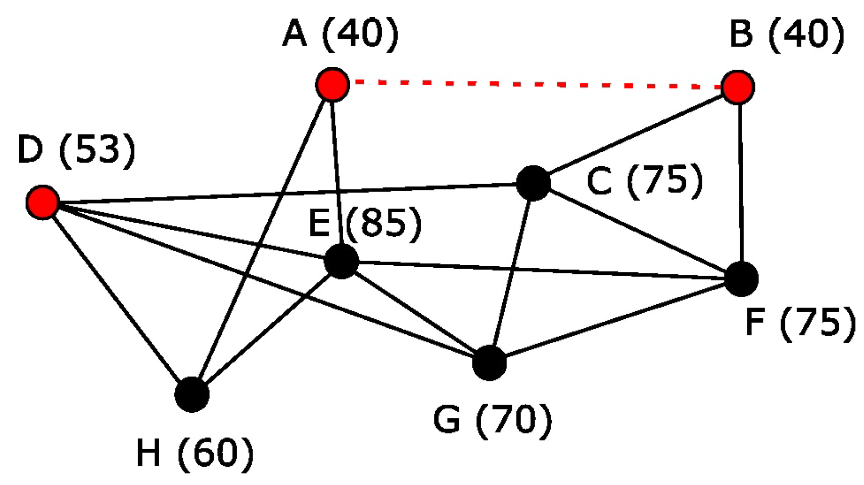
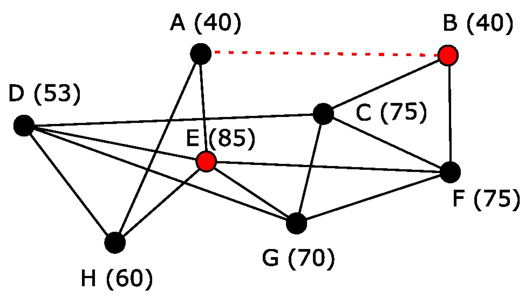
In relation to the defined transportation network, the minimum weighted dominating set found by using Algorithm 4, is determined by the red vertices shown in Figure 2; e.g., $D_w=\{B,D\}$. The weighted domination number is equal to 93. When solving a static problem, we assume that this set is the basis for a new minimal weighted dominating set.

Using the weighted bondage-connected number as a parameter of weighted structural vulnerability, we can conclude that in case 1 (dynamic case) it is enough to remove the red dotted edge $\{A,B\}$ for the weighted domination number to increase to 133 Figure 3.

However, if we consider a dynamic case in which after the edge removal operation, we are again looking for the minimal dominating set, then we can conclude that the value of the weighted structural vulnerability parameter is 1, and, as in the first case, removal of the red dotted edge $\{A,B\}$ is enough to weighted domination number increased to 125 instead of the nominal 93, see as Figure 4.

5. Conclusions

In the paper, six new vulnerability indicators of transport networks have been proposed. Every one of them is based on the domination concepts and related topics; e.g., bondage number and domination subdivision number. Two new algorithms have been introduced as the tools for calculating the values of the parameters defined. These algorithms will work well for small networks but may need more time for large-scale ones. The methods given in the article are universal and applicable to both small- and large-scale networks. Moreover, the presented approach can support the dynamic analysis of bottlenecks in transport networks.

References

- Croatian Parliament. Croatian Law on Critical Infrastructures; Official Gazette: Zagreb, Croatia, 2013. [Google Scholar]
- European Union; European Commission. Communication from the Commission on Critical Infrastructure Protection in the Fight Against Terrorism; COM (2004)702 Final; European Union; European Commission: Brussels, Belgium, 2004. [Google Scholar]
- European Union; European Commission. Green Paper on a European Program for Critical Infrastructure Protection; COM (2005)576 Final; European Union; European Commission: Brussels, Belgium, 2005. [Google Scholar]
- European Union; European Council. Council Directive 2008/114/EC of 8 December 2008 on the Identification and Designation of European Critical Infrastructures and the Assessment of the Need to Improve Their Protection; European Union; European Council: Brussels, Belgium, 2008. [Google Scholar]
- US President’s Commission on Critical Infrastructure Protection. Critical Foundations: Protecting America’s Infrastructures; US President’s Commission on Critical Infrastructure Protection: Washington, DC, USA, 1997. [Google Scholar]
- Kolowrocki, K.; Soszyńska-Budny, J. Reliability and Safety of Complex Technical Systems and Processes, Modeling-Identification-Prediction-Optimization; Springer Series in Reliability Engineering; Springer: Berlin/Heidelberg, Germany, 2011. [Google Scholar]
- Borkowski, P. Inference engine in an intelligent ship course-keeping system. Comput. Intell. Neurosci. 2017, 2017. [Google Scholar] [CrossRef] [Green Version]
- Blokus, A.; Kolowrocki, K. Reliability and maintenance strategy for systems with aging-dependent components. Qual. Reliab. Eng. Int. 2019, 35, 2709–2731. [Google Scholar] [CrossRef]
- Bogalecka, M.; Kolowrocki, K.; Soszynska-Budny, J. A General Approach to Critical Infrastructure Accident Consequences Analysis. In Proceedings of the International Conference on Numerical Analysis and Applied Mathematics 2015 (ICNAAM-2015), Rhodes, Greece, 23–29 September 2015. [Google Scholar]
- Levina, E.; Tirpak, D. Adaptation to Climate Change: Key Terms; Organisation for Economic Co-operation and Development (OECD): Paris, France, 2006. [Google Scholar]
- US Department of Homeland Security. National Infrastructure Protection Plan (NIPP) 2013: Partnering for Critical Infrastructure Security and Resilience; US Department of Homeland Security: Washington, DC, USA, 2013. [Google Scholar]
- Kolowrocki, K.; Soszynska-Budny, J.; Torbicki, M. Critical Infrastructure Impacted by Climate Change Safety and Resilience Indicators. In Proceedings of the IEEE International Conference on Industrial Engineering and Engineering Management (IEEE IEEM), Bangkok, Thailand, 16–19 December 2018; pp. 986–990. [Google Scholar]
- Borkowski, P. Numerical modeling of wave disturbances in the process of ship movement control. Algorithms 2018, 11, 130. [Google Scholar] [CrossRef] [Green Version]
- Guze, S. Business Availability Indicators of Critical Infrastructures Related to the Climate-Weather Change. In Contemporary Complex Systems and Their Dependability, DepCoS-RELCOMEX 2018; Zamojski, W., Mazurkiewicz, J., Sugier, J., Walkowiak, T., Kacprzyk, J., Eds.; Springer: Cham, Switzerland, 2019. [Google Scholar]
- Newell, G.F. Traffic Flow on Transportation Networks; Series in Transportation Studies; MIT Press: London, UK, 1980. [Google Scholar]
- Blokus-Roszkowska, A.; Smolarek, L. Maritime traffic flow simulation in the Intelligent Transportation Systems. In Proceedings of the European Safety and Reliability Conference (Esrel): Safety and Reliability: Methodology and Applications, Wrocław, Polska, 14–18 September 2014; pp. 265–274. [Google Scholar]
- Rodrigue, J.P.; Comtois, C.; Slack, B. The Geography of transport Systems, 4th ed.; Routledge: London, UK, 2017. [Google Scholar]
- Cascetta, E. Transportation Systems in Transportation Systems Engineering: Theory and Methods; Springer: Boston, MA, USA, 2001. [Google Scholar]
- Haładyn, S.M.; Restel, F.J.; Wolniewicz, L. Method for railway timetable evaluation in terms of random infrastructure load. In Proceedings of the Fourteenth International Conference on Dependability of Computer Systems DepCoS-RELCOMEX, Brunów, Poland, 1–5 July 2019. [Google Scholar]
- Friedrich, J.; Restel, F.J. A fuzzy approach for evaluation of reconfiguration actions after unwanted events in the railway system. In Proceedings of the Fourteenth International Conference on Dependability of Computer Systems DepCoS-RELCOMEX, Brunów, Poland, 1–5 July 2019; pp. 195–204. [Google Scholar]
- Restel, F.J. Train punctuality model for a selected part of railway transportation system. In Safety, Reliability and Risk Analysis: Beyond the Horizon: Proceedings of the European Safety and Reliability Conference, Amsterdam, The Netherlands, 29 September–2 October 2013; CRC Press: Steenbergen, The Netherlands, 2014; pp. 3013–3019. [Google Scholar]
- Ding, X.; Guan, S.; Sun, D.J.; Jia, L. Short Turning Pattern for Relieving Metro Congestion during Peak Hours. Eur. Transp. Res. Rev. 2018, 2018, 1–11. [Google Scholar]
- Harrary, F. Graph Theory; Addison-Wesley: Boston, MA, USA, 1969. [Google Scholar]
- Van Leeuwen, J. Chapter 10—Graph Algorithms Book–Algorithms and Complexity. In Handbook of Theoretical Computer Science; MIT Press: Cambridge, MA, USA, 1990; Volume 525, pp. 527–631. [Google Scholar]
- Gross, J.L.; Yellen, J. Handbook of Graph Theory; CRC Press: Boca Raton, FL, USA, 2004; ISBN 978-1-58488-090-5. [Google Scholar]
- Kansky, K.J. The Structure of Transport Networks; University of Chicago: Chicago, IL, USA, 1963. [Google Scholar]
- Haynes, T.W.; Hedetniemi, S.; Slater, P. Fundamentals of Domination in Graphs; CRC Press: Boca Raton, FL, USA, 1998. [Google Scholar]
- Velammal, S. Studies in Graph Theory: Covering, Independence, Domination and Related Topics. Ph.D. Thesis, Manonmaniam Sundaranar University, Tirunelveli, India, 1997. [Google Scholar]
- Haynes, T.W.; Hedetniemi, M.; Hedetniemi, T. Domination and independence subdivision numbers of graphs. Discuss. Math. Graph Theory 2000, 20, 271–280. [Google Scholar] [CrossRef] [Green Version]
- Guze, S. Graph Theory Approach to Transportation Systems Design and Optimization. Int. J. Mar. Navig. Saf. Sea Transp. 2014, 8, 571–578. [Google Scholar] [CrossRef] [Green Version]
- Guze, S. An application of the selected graph theory domination concepts to transportation networks modelling. Sci. J. Marit. 2017, 52, 97–102. [Google Scholar]
- Bhattacharya, A.; Vijayakumar, G.R. Effect of edge-subdivision on vertex-domination in a graph. Discuss. Math. Graph Theory 2002, 22, 335–347. [Google Scholar] [CrossRef] [Green Version]
- Walikar, H.B.; Acharya, B.D.; Sampathkumar, E. Recent Developments in the Theory of Domination in Graphs; Mehta Research Institute of Mathematics: Allahabad, India, 1979; Volume 1, Available online: https://www.tib.eu/en/search/id/TIBKAT%3A014901056/Recent-developments-in-the-theoryof-domination/ (accessed on 11 December 2019).
- Parekh, A.K. Analysis of Greedy Heuristic for Finding Small Dominating Sets in Graphs. Inf. Process. Lett. 1991, 39, 237–240. [Google Scholar] [CrossRef] [Green Version]
- Ruan, L.; Du, H.; Jia, X.; Wu, W.; Li, Y.; Ko, K.-I. A greedy approximation for minimum connected dominating sets. Theor. Comput. Sci. 2004, 329, 325–330. [Google Scholar] [CrossRef] [Green Version]
- Topp, J. Graph with unique minimum edge dominating sets and graphs with unique maximum independent sets of vertices. Discret. Math. 1993, 121, 199–210. [Google Scholar] [CrossRef] [Green Version]
- Fink, J.F.; Jacobson, M.S.; Kinch, L.F.; Roberts, J. The bondage number of graph. Discret. Math. 1990, 86, 47–57. [Google Scholar] [CrossRef] [Green Version]
- Hartnell, B.L.; Rall, D.F. Bounds on the bondage number of a graph. Discret. Math. 1994, 128, 173–177. [Google Scholar] [CrossRef] [Green Version]
- Detalaff, M.; Raczek, J.; Topp, J. Domination Subdivision and Domination Multisubdivision Numbers of Graphs. Discuss. Math. Graph Theory 2019, 39, 829–839. [Google Scholar] [CrossRef]
- Berdica, K. An introduction to road vulnerability: What has been done, is done and should be done. Transp. Policy 2002, 9, 117–127. [Google Scholar] [CrossRef]
- Appert, M.; Chapelon, L. Measuring Urban Road Network Vulnerability using Graph Theory: The Case of Montpellier’s Road Network. Working Paper. 2013, pp. 1–8. Available online: https://halshs.archives-ouvertes.fr/halshs-00841520/document (accessed on 30 November 2019).
- Berdica, K.; Eliasson, J. Regional accessibility analysis from a vulnerability perspectiv. In Proceedings of the Second International Symposium on Transportation Network Reliability (INSTR), Christchurch and Queenstown, New Zealand, 20–24 August 2004; pp. 89–94. [Google Scholar]
- D’Este, G.M.; Taylor, M.A.P. Network vulnerability: An approach to reliability analysis at the level of national strategic transport networks. In The Network Reliability of Transport, Emerald Group Publishing Limited; Bell, M., Iida, Y., Eds.; Pergamon: Oxford, UK, 2003; pp. 23–44. [Google Scholar] [CrossRef]
- Du, Z.P.; Nicholson, A. Degradable transportation systems: Sensitivity and reliability analysis. Transp. Res. Part Methodol. 1997, 31, 225–237. [Google Scholar] [CrossRef]
- Husdal, J. Reliability and vulnerability versus cost and benefits. In Proceedings of the Second International Symposium on Transportation Network Reliability (INSTR), Christchurch, New Zealand, 20–24 August 2004; pp. 182–188. [Google Scholar]
- Immers, L.H.; Stada, J.E.; Yperman, I.; Bleukx, A. Robustness and resilience of transportation networks. In Proceedings of the 9th International Scientific Conference MOBILITA, Bratislava, Slovenia, 6–7 May 2004. [Google Scholar]
- Jenelius, E.; Petersen, T.; Mattsson, L. Importance and exposure in road network vulnerability analysis. Transp. Res. Part A 2006, 40, 537–560. [Google Scholar] [CrossRef]
- Reggiani, A.; Nijkamp, P.; Lanzi, D. Transport resilience and vulnerability: The role of connectivity. Transp. Res. 2015, 81, 4–15. [Google Scholar] [CrossRef]
- Sarewitz, D.; Pielke, R., Jr.; Keykhah, M. Vulnerability and risk: Some thoughts from a political and policy perspective. Risk Anal. 2003, 23, 805–810. [Google Scholar] [CrossRef] [Green Version]
- Sun, D.; Zhao, Y.; Lu, Q.-C. Vulnerability Analysis of Urban Rail Transit Networks: A Case Study of Shanghai, China. Sustainability 2015, 7, 6919–6936. [Google Scholar] [CrossRef] [Green Version]
- Sun, D.; Guan, S. Measuring vulnerability of Urban Metro Network from Line Operation Perspective. Transp. Res. 2016, 94, 348–359. [Google Scholar] [CrossRef]
- Estrada, E. Network robustness to targeted attacks. The interplay of expansibility and degree distribution. Eur. Phys. J. 2006, 52, 563–574. [Google Scholar] [CrossRef]
- Latora, V.; Marchiori, M. Vulnerability and protection of infrastructure networks. arXiv 2004, arXiv:cond-mat/0407491v1. [Google Scholar] [CrossRef] [PubMed] [Green Version]
- Hollnagel, E.; Woods, D.D.; Leveson, N. Resilience Engineering: Concepts and Percepts; Ashgate Publishing Limited: Aldershot, UK, 2006. [Google Scholar]
- Patriarca, R.; Bergström, J.; Di Gravio, G.; Costantino, F. Resilience engineering: Current status of the research and future challenges. Saf. Sci. 2018, 102, 79–100. [Google Scholar] [CrossRef]
Figure 1.
Exemplary weighted transportation network; weights describe the red light time.
Figure 2.
Minimal weighted dominating set in considered network, .
Figure 3.
Weighted bondage-connected number in transportation network with fixed weighted dominating set, .
Figure 4.
Weighted bondage-connected number in transportation network without fixed weighted dominating set, .
© 2019 by the author. Licensee MDPI, Basel, Switzerland. This article is an open access article distributed under the terms and conditions of the Creative Commons Attribution (CC BY) license (http://creativecommons.org/licenses/by/4.0/).
Share and Cite
MDPI and ACS Style
Guze, S. Graph Theory Approach to the Vulnerability of Transportation Networks. Algorithms 2019, 12, 270. https://0-doi-org.brum.beds.ac.uk/10.3390/a12120270
AMA Style
Guze S. Graph Theory Approach to the Vulnerability of Transportation Networks. Algorithms. 2019; 12(12):270. https://0-doi-org.brum.beds.ac.uk/10.3390/a12120270
Chicago/Turabian StyleGuze, Sambor. 2019. "Graph Theory Approach to the Vulnerability of Transportation Networks" Algorithms 12, no. 12: 270. https://0-doi-org.brum.beds.ac.uk/10.3390/a12120270
Note that from the first issue of 2016, this journal uses article numbers instead of page numbers. See further details here.