Research on Quantitative Investment Strategies Based on Deep Learning


1
SHU-UTS SILC Business School, Shanghai University, Shanghai 201899, China
2
Carey Business School, The Johns Hopkins University, Baltimore, MD 20036, USA
3
Smart City Research Institute, Shanghai University, Shanghai 201899, China
*
Author to whom correspondence should be addressed.
Algorithms 2019, 12(2), 35; https://0-doi-org.brum.beds.ac.uk/10.3390/a12020035
Submission received: 5 January 2019
/
Revised: 2 February 2019
/
Accepted: 9 February 2019
/
Published: 12 February 2019
Abstract
:This paper takes 50 ETF options in the options market with high transaction complexity as the research goal. The Random Forest (RF) model, the Long Short-Term Memory network (LSTM) model, and the Support Vector Regression (SVR) model are used to predict 50 ETF price. Firstly, the original quantitative investment strategy is taken as the research object, and the 15 min trading frequency, which is more in line with the actual trading situation, is used, and then the Delta hedging concept of the options is introduced to control the risk of the quantitative investment strategy, to achieve the 15 min hedging strategy. Secondly, the final transaction price, buy price, highest price, lowest price, volume, historical volatility, and the implied volatility of the time segment marked with 50 ETF are the seven key factors affecting the price of 50 ETF. Then, two different types of LSTM-SVR models, LSTM-SVR I and LSTM-SVR II, are used to predict the final transaction price of the 50 ETF in the next time segment. In LSTM-SVR I model, the output of LSTM and seven key factors are combined as the input of SVR model. In LSTM-SVR II model, the hidden state vectors of LSTM and seven key factors are combined as the inputs of the SVR model. The results of the two LSTM-SVR models are compared with each other, and the better one is applied to the trading strategy. Finally, the benefit of the deep learning-based quantitative investment strategy, the resilience, and the maximum drawdown are used as indicators to judge the pros and cons of the research results. The accuracy and deviations of the LSTM-SVR prediction models are compared with those of the LSTM model and those of the RF model. The experimental results show that the quantitative investment strategy based on deep learning has higher returns than the traditional quantitative investment strategy, the yield curve is more stable, and the anti-fall performance is better.
1. Introduction
Financial innovation improvement drives the rise of quantitative trading in the Chinese financial market. As major parts of the national market economy, the crucial roles stocks, futures, and options markets attract an increasing number of researchers for the study of market price behavior. Instead of introducing numerous premise assumptions, the adoption of deep learning techniques makes it possible to directly hand over rules mining tasks to computers. In this way, the study of stocks, futures and options price behavior is essentially a predictive work that is related to the future price trend of trading objects in the market.
At present, most researches target the stock market [1,2,3], however, in China, traders can only buy stocks first, which means that traders can only hold a long position. Besides, T + 0 trading is also forbidden, which means traders cannot sell the amount of stocks they bought within a same day. These rules contribute to the particularity of Chinese stock market, which further negatively prompts the utilization of prediction based on deep learning in this realm. Therefore, this article focuses on an options market with four trading strategies (Long Call, Short Call, Long Put, Short Put) where deep learning prediction results can be fully employed, in order to mirror the impact of its accuracy on quantitative trading strategies in a straightforward way.
However, financial markets tend to present tremendous noise, non-stationarity, and non-linearity [4,5,6]. Furthermore, technical indicators of the traditional financial market cannot fully reflect the situation, which lead to problems such as greater delay and lower accuracy. Meanwhile, conventional econometric equations hardly perform well in analyzing high-dimensional, complex, and noisy financial market data. In sharp contrast, deep learning-based data mining models succeed in avoiding drawbacks mentioned above, and they are more likely to obtain a more accurate result [5].
Deep learning models [7] have attracted huge attention from researchers and investors, due to their superiority in dealing with extremely complex problems [2,5]. Many high-tech companies, such as Microsoft, Baidu, and Google, have already invested heavily in deep learning models, in order to take leading positions.
Financial market prediction is actually a high-dimensional time series forecast, since differences always exist between contiguous moments. For time-series forecasting, Passalis et al. [8] proposed a novel temporal-aware neural bag-of-features (BoF) model, which is tailored to the needs of time-series forecasting by using high frequency limit order book data that captures both long-term and short-term behavior in order to handle the complex situation and to improve the prediction ability. Researchers have already discussed quite a few econometrical and statistical models, such as the Autoregressive Integrated Moving Average (ARIMA) model [9] and the Vector Autoregressive (VAR) model [10] etc., in financial time series predictions, but these models cannot perfectly fit the financial time series, due to their non-stationarity and nonlinearity. Given these characteristics, researchers have subsequently turned to artificial neural networks (ANNs) [11], deep learning [6,12], and other models. Results show that these models perform better in reflecting real financial situations compared to the linear ones. Based on the structural risk minimization principle, Support Vector Machine (SVM) is an approach that involves training of the polynomial or radial basis function neural network. Compared with other methods, it has better generalization performance [13], which has gained favor from numerous researchers. For instance, Kim [4] and Sun [14] took advantage of SVM for financial forecasting, and both achieved good results. However, one model approach may ignore other features of the problem, which brings about the multiple models approach. Van [15] and Das [16] etc., all combine a variety of models to enhance prediction results by exploiting the characteristics of each model. The application of deep learning in financial markets not only lowers the difficulty of analysis and forecasting to a large extent, but also introduces new investment methods and ideas to investors.
Based on the above ideas, this paper will adopt the deep learning and support vector machine approach, as well as using the specific data (50 ETF options data) to predict the 50 ETF price. During the research, the data is preprocessed, which involves the following procedures. First of all, the History Volatility (HV) model and the Implied Volatility (IV) model are combined to calculate the HV of 50 ETF and the IV of 50 ETF options. Then, they are selected as two input characteristics of the deep learning model, and the price prediction model of the 50 ETF options is constructed. Afterwards, the question of whether the deep learning shows a higher accuracy rate on this problem is studied, as well as whether the quantitative investment strategy can lead to a higher rate of return and lower drawdown.
The experimental results show that compared with the traditional quantitative investment strategy, the quantitative investment strategy based on deep learning presents higher returns, a more stable yield curve, and better anti-fall performance. Therefore, the quantitative investment strategy based on deep learning has certain reference value for investors when making decisions. For the deep learning model, the Long Short-Term Memory (LSTM) that is built in this paper, there is still space to improve, and the combined Long Short-Term Memory– Support Vector Regression (LSTM-SVR) model improves significantly in prediction accuracy. At the same time, the quantitative investment strategy developed in this paper can withstand certain prediction errors, so that the quantitative investment strategy based on deep learning in this paper has a better performance in the options market. In contrast, in the stock and futures markets, errors are likely to cause huge losses. For the stock market, due to the particularity of China’s stock market, only T + 1 trading transactions can be conducted, and this error may result in a certain amount of loss. With regard to the futures market, the loss caused by the error may even lead to a direct burst. Therefore, there is still a lot of work that needs to be done in research on quantitative investment strategies based on deep learning.
The innovative points of this paper are as follows: (1) Based on the deep learning model LSTM, this paper combines LSTM and SVM to form the LSTM-SVR model. This model can reduce the predicted deviation value; that is, improve the accuracy of the prediction, especially during a relatively stable period. (2) The quantitative investment strategy designed in this paper introduces the concept of hedging, which guarantees Delta neutrality. The experiment proves that hedging boosts the quantitative investment strategy performance in terms of profitability and stability. (3) The quantitative investment strategy in this paper is conducted every 15 minutes, which is closer to the real trading market, so that the back-testing results can be more practical. (4) This paper combines the prediction result of the deep learning model LSTM-SVR, which acts as a signal ‘diff’ with the quantitative investment strategy to form a quantitative investment strategy based on the deep learning model, which exhibits a distinct optimization in terms of both yield and resilience.
The paper is organized as follows: Section 2 offers a brief review of both the related domestic and foreign literature. Section 3 introduces the models and the quantitative investment strategy of this paper. Section 4 introduces the experimental simulation. Section 5 analyzes and compares the experimental results. Section 6 gives conclusions and prospects.
2. Literature Review
Quantitative investment strategies can be currently divided into single model-based research and multi-model-based ones. Due to advantages in solving complex and non-linear problems, more researches are conducted by adopting deep learning methods. Additionally, multi-model based methods can produce higher accuracies than the single-model ones, providing both theoretical and practical significance.
In terms of single models, researchers have proposed a number of instructive studies. Kercheval et al. [17] proposed a framework based on machine learning to acquire the dynamics of high-frequency limit-order books in financial equity markets, and to predict the real-time metrics automatically. They used multi-class support vector machines to help build a learning model for each metric. They found that it is effective to forecast the short-term price by using the features from the proposed framework. Fan and Palaniswami [18] studied the stock selection problem by using support vector machines (SVM) to identify stocks that are likely to receive excess returns and to outperform the market. The total return of the equal-weight stocks portfolio selected by SVM over a five-year period was 208%, which remarkably exceeded the benchmark of 71%. They found that through a class sensitivity tradeoff, the output of the support vector machine can be interpreted as a probability measure and sorted, so that the selected stock can be fixed at the top 25%. Although traditional SVM can reach good results, it is still necessary to improve the common method for better results when dealing with some special problems. Tay and Cao [13] proposed an improved model, the C-ascending support vector machine, and applied it for simulating non-stationary financial time series. Based on prior knowledge, the dependence between input variables and output variables changed over time. Specifically, recent past data can provide more important information than distant past data. They exposed that this support vector machine had a better prediction ability than the traditional SVM when handling the actual ordered sample data. Cao and Tay [19] studied the application of SVM in financial time series predictions, and compared it with the multi-layer back-propagation neural network (BPNN) and the regularized radial basis function neural network (RBF). The application feasibility of the support vector machine in financial forecasting was studied, and the variation of support vector machine performance with free parameters was studied. Introducing the non-stationarity financial time series into the support vector machine, they put forward adaptive parameters, which had higher generalization performances in financial forecasting. However, for single models, one-sidedness learning features still exist; that is, it is impossible to learn the important features comprehensively, resulting in poor prediction results.
Therefore, in order to fully characterize the features, researchers combined two or more models to form a hybrid one, for a more outstanding performance. Lin et al. [20] proposed an approach based on particle swarm optimization for parameter determination and feature selection of the SVM, called particle swarm optimization + support vector machine (PSO-SVM). In order to evaluate it, multiple common data sets were used to calculate the classification accuracy, where the PSO-SVM method was compared with the traditional parameter value grid search method and other methods. Results showed that the classification accuracy of this method outperforms other methods, and achieves similar results to the GA-SVM method, which illustrates that the PSO-SVM method is valuable for parameter determination and feature selection of support vector machines. Das and Padhy [16] further improved on the basis of Lin, linking SVM with teaching–learning-based optimization (TLBO) which avoids user-specified control parameters that are required in other optimization methods. The feasibility and effectiveness of this hybrid model was evaluated by predicting the daily closing price of the Commodity Futures Index (COMDEX). They discovered that this model is more efficient than the PSO-SVM hybrid model and the standard support vector machine model. Hsu [21] designed a hybrid method based on back-propagation neural network (BPNN), feature selection technology and genetic programming (GP), using technical indicators to solve the stock/future price forecasting problem. By predicting the closing price of the spot monthly futures of the Taiwan Stock Exchange’s Capital Weighted Index (TAIEX), the feasibility and effectiveness of the forecast are verified. In addition, the most important technical indicators can be determined by using a feature selection method based on the proposed simulation technique, or a preliminary GP prediction model. Liang et al. [22] proposed a simple and effective options price prediction method based on neural network (NN) and SVR analysis. First, they improved the traditional options pricing method to make options prices prediction accessible. Secondly, the use of NNs and SVRs further reduced the prediction error of the parametric method. Since the traditional method simulated the trend of the actual options price, the prediction error of the nonlinear curve simulated in a mixed model of NNs and SVRs in the first stage can be further reduced in the second stage. Finally, a lot of experimental research on the Hong Kong options market data proved that NNs and SVRs can improve the prediction accuracy.
With the further development of deep learning, researchers have also applied it into the financial forecasting field, where financial time series forecasting problems are also essentially time series problems. Considering that the performance of Recurrent Neural Networks (RNN) tend to surpass other methods, many researchers have focused their attention on RNN. Tsantekidis et al. [23] used recurrent neural networks to form a deep learning methodology to forecast the price movement in future by using large-scale high-frequency data on Limit Order Books. Chen et al. [24] modeled and predicted China stock returns by using LSTM. Compared with the random prediction method, the proposed LSTM model showed its power by improving the accuracy of the stock returns forecast. Minami [25] proposed a sequential learning model that uses LTSM-RNN methods to predict individual stock prices with corporate behavioral event information and macroeconomic indices, displaying broad application prospects in stock price forecasting under the corporate behavior and corporate publishing variables. Besides, some researchers used other deep learning models; Tsantekidis et al. [26] used Convolutional Neural Networks (CNNs) to form a deep learning methodology to forecast the price movements of stocks, using as input large-scale, high-frequency time-series derived from the order book of financial exchanges. Tsantekidis et al. compared CNNs with other models like SVM and Multilateral Neural Networks to show that CNNs had better performance in their situation. However, compared with hybrid models, single models are usually unlikely to give a best result. Hence, Sun et al. [6] proposed a hybrid integration learning method of the AdaBoost model and the LSTM network to predict financial time series. The database was trained by AdaBoost model to obtain training samples, after which each of them was predicted by LSTM. Finally, the prediction results of all LSTM predictors were synthesized by the AdaBoost model to offer an integrated result. This AdaBoost-LSTM integrated learning method was illustrated to be superior to other single prediction models and integrated learning methods.
In this paper, two different LSTM-SVR models are proposed to forecast the 50 ETF price. Through studying the 50 ETF options market in the Chinese options market, this paper aims to design a short-strangle quantitative investment strategy based on the historical volatility and the implied volatility of 50 ETF underlying goods. The trading frequency is every 15 min (daily trading 16 times), and the concept of hedging is introduced to keep Delta neutral, so that more stable returns can be gained under stable market conditions. Then, the LSTM-SVR hybrid models (LSTM-SVR I and LSTM-SVR II) are used to predict the future price of the 50 ETF target, and the accuracy and error of the prediction results of these two models are compared in this paper. Results show that the LSTM-SVR I model has better performance than the LSTM-SVR II model. Therefore, the results of the LSTM-SVR I model are added into trading strategy. The prediction results based on the deep learning model LSTM-SVR I are further viewed as an investment signal diff, which is added into the quantitative investment strategy in this paper for greater returns and better resilience.
The following section will introduce the models and the quantitative investment strategy.
3. Models and Quantitative Investment Strategy
3.1. Long Short-Term Memory (LSTM) Model
Sepp Hochreiter and Jurgen Schmidhuber [27] first proposed the LSTM model in 1997. The LSTM neural network is a new deep learning neural network based on the Recurrent Neural Networks (RNN) model. Therefore, before introducing the LSTM model, we need to introduce the RNN model.
It can be seen from Figure 1 that compared with ANNs, in addition to the input and output layer, the RNN model also considers the hidden layer at the next time step. Through the feedback of the hidden layer at this time step, the weight of the hidden layer at the next time step is affected. The RNN model is often simplified to the right part of Figure 1 for better understanding. In the RNN model, the next time is affected by the current time . It is worth noting that the weights at each time step (including weights from the input layer to the hidden layer and from the hidden layer to the output layer) are the same. After the RNN model is expanded according to the time steps, the structure of Figure 2 can be obtained:
Where w1 means the weight input from the output layer to hidden layer at the same time. w2 means the weight input from last hidden layer to next hidden layer at adjacent time points. w3 means the weight input from the hidden layer to the input layer at the same time.
After expanding the RNN model, it is possible to analyze and understand its structure in a much more clear way. Forward propagation can be calculated according to the time sequence, as shown in Figure 3, whereas back-propagation refers to passing the accumulated residuals forward and correcting the weights, which start from the last time step, as shown in Figure 4. Therefore, back-propagation enables the RNN model to perform end-to-end training.
Forward Propagation:
The RNN model and its formula in this paper are cited from [28], where b refers to the value calculated by the activation function, refers to the value calculated by the aggregation, w represents the weights connecting different nodes, w with the subscript k is associated with the output layer, and w with the subscript h is associated with the hidden layer, and a function with parentheses indicates the activation function. As seen from the above equation, similar to the normal neural network, the output layer in the RNN model is also the sum of the product of the hidden layers output and its weights. Yet, the difference is that all the calculated values have time nodes t as a superscript, which indicates the time t. L represents the Loss Function, which is the mean squared error. The formula of the Loss Function is:
where is the actual value and is the fit value.
The difference between the RNN model and the traditional neural networks model mentioned above is that the hidden layer receives the data from the hidden layer of the previous time, which can also be reflected in Equation (2). The first summation in Equation (2) represents the result from the input layer, which is the same as the traditional neural network, while the second summation represents the result from the hidden layer of the previous time. Finally, the result of the activation function in Equation (3) is substituted into Equation (1) to calculate the final result through the summation process.
Back-propagation:
The above formula mainly calculates the cumulative residual in the hidden layer during back-propagation. Similar to the forward propagation, the two parts in the second bracket of the right part in Equation (5) represent the residual returned by the output layer at present, and the residual returned by the hidden layer of the next time step (because it is back-propagated). In order to achieve the fastest gradient descent, the two values are derived to correct the weights of each node.
For the RNN model, in the process of minimizing Loss, the Loss Function needs to be derived (computing the gradient), since the gradient direction (the direction of the derivation) is the fastest direction in which the value of the Loss Function decreases. However, when computing the gradient of the Loss Function, Gradient Vanish phenomenon is likely to happen. That is to say in the process of finding the minimum value, the gradient function disappears quickly. As a result, the Loss Function requires nearly infinite time to approach the minimum value.
Although simple, the traditional way to solve the Gradient Vanish that replaces the activation is still effective. However, a better model architecture can help to significantly correct and optimize RNN. Thus, Sepp Hochreiter and Jurgen Schmidhuber [27] proposed the LSTM model.
In order to solve problems exposed in the RNN model, the LSTM model adds a long-time lag. In the structure shown in Figure 5, each memory cell is controlled by three special gates for reading, writing and saving functions. These three types of gates are called the forget gate, the output gate and that input gate, respectively, which only have weights of 0 and 1 to selectively correct the parameters. For example, when the weight of the forget gate is 1, the storage cell stores the content information, while when the forget gate has a weight of 0, the storage cell clears the previous content. When the weight of the input gate is 1, new information will be sent to the memory cell, whereas when the weight is 0, no information will enter the memory cell. When the weight of the output gate is 1, the information stored in the memory cells is accessible to the other parts of the LSTM.
For the model shown in Figure 5, the values of the three gates for each memory cell are obtained through training. Each black node in Figure 5 represents an associated activation function. The commonly used activation function is the sigmoid function. In forward propagation, the calculation formula for each department is as follows [29]:
Input gate:
The subscript L is related to the input gate. According to Equation (8), the input of the input gate includes the input of the outer layer and the dashed line from the memory cells, which is expressed as the first summation and the third summation part of the right side of the Equation in Equation (8). The second part of the summation with H can be seen as part of the input from the outer layer, which can either be the result of the interconnection between the memory cells or the result of the interconnection between the hidden layers, reflecting the flexibility of LSTM. The subscript c is related to the memory cells.
Forget gate:
Inputs associated with the forget gate include: the inputs from the outer layer, the memory cells (dashed line) and the input layer.
Memory cells:
where is the network’s cell state at the time t. As can be seen from Equation (12), the inputs associated with memory cells include: the general inputs of the outer layer and the input layer. in Equation (13) represents an activation function, and Equation (13) shows that the memory cells connect the product of the forget gate and the previous time state, and the product of the input gate and the activation function, which are then summed.
Output gate:
The output layer shares the same principle of the input layer.
The final output is:
The small black dot above the LSTM structure diagram is another activation function .
Back propagation:
Input gate:
Forget gate:
Output gate:
Memory cells:
Final output:
In conclusion, the invention of LSTM solves the problem that the weight of the training becomes very small due to the disappearance of the gradient when the RNN is back-propagating, which further causes that the whole training process to only reach a local optimal solution. Through adding three gates (the input gate, output gate, and forget gate), the LSTM solves this problem and assists in controlling the error during propagation, which ensures that a gradient explosion will never occur, regardless of the diversity of the spread. Therefore, this paper adopts the LSTM model for research.
Based on the data obtained from the database and the data obtained through data processing, this paper sorts out input data with seven attributes: the final transaction price within the 50 ETF time segment, the purchase price (the highest bid price within the time segment on the market), the highest price within the 50 ETF time segment, the lowest price within the 50 ETF time segment, the volume within the time segment, the historical volatility (HV) at that time, and the implied volatility (IV). These seven features are stored as independent variables in the csv file, and Tensorflow is used to build the LSTM cell in Python. Under the Python 3.6 environment, the deep learning model LSTM is run with seven features as input data. Under MATLAB, the Random Forest (RF) model proposed in paper [30] is built with seven features as input data. Compared with the result of LSTM and the result of RF, LSTM shows better performance. Therefore, LSTM is chosen to combine with SVR. At the same time, the traditional machine learning model, SVR, is also adopted. Eight features in total, which involve the seven attributes as well as the predicted values obtained by the LSTM model, are used as the input data of the SVR model in MATLAB, to form the LSTM-SVR I model. Besides, the hidden state vectors from every hidden layers of LSTM are extracted and these hidden vectors with seven attributes are combined as input data of the SVR model to form the LSTM-SVR II model. Since in this paper the hidden units used in LSTM is 20, and as for the LSTM-SVR II model, there are a total of 27 attributes as the inputs of SVR. The support vector regression SVR method in this paper is proposed by.
The following section will introduce quantitative investment strategies.
3.2. The Support Vector Regression Model
Different from the traditional SVM proposed in paper [31] used for classification, in this article, the SVR model proposed in paper [32] is used as a part of the LSTM-SVR model.
The difference between the SVR used in this article and the traditional SVM used for classification includes the objective function, constraint, and kernel function:
As for SVC:
where, represents the margin between the two support vectors, -1=0 denotes the sample on the frontier, and equals 1 or −1.
As for SVR:
where, represents the margin between two support vectors, -1=0 means the sample on the frontier, equals 1 or −1.
In the SVR model, if the difference between the prediction value and the real value is less than the threshold , we will not make a penalty on this sample point.
In the SVR model in this article, RBF (radial basis function) is selected as the kernel function. Therefore, there are two significant parameters, c and g. A detailed discussion of c and g is given a following section (Section 4.3.2).
3.3. Quantitative Investment Strategies
3.3.1. Introduction to the Basics of Options
According to the paper [33], there are the introductions to basics of options:
(1) 50 ETF options
The options used in this article is the Shanghai 50 ETF options. The Shanghai 50 ETF options contract is a standardized contract established by the Shanghai Stock Exchange to provide the buyer with the right to buy or sell the “Shanghai 50 Trading Open Index Securities Investment Fund” at a specific price within a certain period of time. After paying a certain amount of premiums, the buyer of the 50 ETF options has the absolute right to decide whether to execute the contract when the contract expires. In contrast, the seller of the contract that receives the buyer’s premiums must unconditionally obey the buyer’s choice within a certain period and fulfill the promise of this transaction.
(2) Strangle options short-term investment strategy
The basis of the quantitative investment strategy used in this paper is the strangle options short-term investment strategy.
A strangle options investment strategy refers to the sale of a portfolio of options with different strike prices but the same maturity date while selling a call options.
For example, a short strangle options portfolio shown in Table 1 is constructed on one trading day (assuming that the strike price of the at-the-money options is 2.65 yuan):
That is, the sale of a 50 ETF call options expiring in December with a strike price at 2.75 yuan, and at the same time, the sale of a 50 ETF put options expiring in December with strike price at 2.55 yuan.
For this short options portfolio, the gains chart on the maturity date can be drawn as shown in Figure 6:
As can be seen from Figure 6, theoretically, the benefits of this strategy are limited, whereas the potential risks are infinite. When the price of the underlying asset finally falls around the strike price, the portfolio can earn profits. On the contrary, when the price of the underlying asset eventually changes substantially, the portfolio faces a loss. That is to say, when the expiration date is reached, compared with the price at the time of opening the position, if the fluctuation of the 50 ETF price is not large, a profit can be obtained; otherwise, it will cause the loss of a large amount of money. Overall, this strategy is suitable for a relatively stable market.
(3) Margin
During options trading, since this article performs as an options seller who is required to pay for the margin at the transaction, to ensure that the seller can perform the options contract when the buyer executes the options, attention must be paid to the amount of margin that is needed prevent trading troubles that are caused by an insufficient remaining amount (such as the inability to hedge, the need for additional margin, etc.) when opening a position and holding a position. The maintenance margin used in this paper is calculated as follows:
where denotes the premium, denotes the futures margin, and denotes out-of-money value of the options, which is divided into two types, namely the out-of-money value of the call options and the out-of-money value of the put options. The corresponding calculation is as follows:
where is the exercise price of the options contract, is the settlement price of the underlying futures contract, and is the options contract unit.
(4) Delta hedge
This article uses the hedging strategy for Delta hedging.
Delta refers to the ratio of changes in the price of an options to changes in the price of the underlying asset, which is expressed by the following formula:
where represents the price of the options; represents the price of the underlying asset.
Delta actually represents the slope of the options win–loss chart. Figure 7 shows the win–loss chart of an options. The curve represents the relationship between the price of the call options and the price of the underlying asset. The straight line is the tangent of the curve at the point (A, B), whose slope indicates that the price of the underlying asset is A and the value of Delta when the options price is B.
The Delta formula for China’s options market is as follows:
The Delta for non-dividend call options is:
where represents the price of the options at time ; represents the options term; represents the options strike price; represents the risk-free rate of continuous compound interest; represents the volatility of the options; represents the cumulative normal distribution function.
The Delta for non-dividend put options is:
According to what is mentioned above, Delta can be understood as the magnitude of the change in the options price caused by one unit price change of underlying asset. If the Delta of the entire investment strategy portfolio is positive, the decrease of the underlying asset price will bring about losses; if the Delta of the entire investment strategy portfolio is negative, the increase of the underlying asset price will lead to losses. Therefore, in order to avoid the loss caused by the fluctuation of the price of the target price, the Delta hedge adjustment is performed at each time stamp to ensure that the Delta of the strategy combination is 0; that is, the Delta neutrality is guaranteed, so that the seller can completely convert premiums into profits on the expiration date, which can be understood as earning time value and abandoning the benefits and losses caused by the price fluctuations.
3.3.2. Introduction to Quantitative Investment Strategies
The logic of the quantitative investment strategy used in this paper is as follows:
(1) The time series of the IV-HV difference between the implied volatility (IV) and the historical volatility (HV) is calculated at 14:55 on the options expiration date. This time series is the IV-HV series for 20 trading days prior to the expiration date.
(2) Sort the IV-HV time series in ascending order and find its 90th percentile as the opening threshold, “option_open”. Find the median the IV-HV time series as the regression closing threshold, “option_close”.
(3) Each transaction timestamp calculates the IV-HV value at that moment, and it is compared with “option_open”. If it is greater than or equal to “option_open”, the position is opened at the amount of 50% of 10 million (considering that the late delta hedge adjustment position will make the margin change and try to ensure that there will be no burst; 50% is reserved); that is, using five million funds to sell a strangle options portfolio based on the options’s maintenance margin. Otherwise, do not open the position.
(4) Under the position circumstance, the Delta hedge adjustment is performed at each timestamp to ensure that the Delta of the strangle options portfolio remains neutral.
(5) The condition of the closing position is that in the case of a position, the IV-HV at that time is smaller than or equal to “option_close”, then “returning the position”. Alternatively, when the price of the 50 ETF at that time is not within the range of the strike price of the options (less than the strike price of the put options or greater than the strike price of the call options), the “stop loss liquidation” is performed. Both “returning the position” and “stopping the position” need to be closed with the opponent price at the moment.
(6) If it is an empty position (including closing the position after opening the position or opening the position all the time) and it has not reached the next expiration date, continue to judge whether each transaction timestamp reaches the opening condition.
(7) If the position is still held on the expiration date, judge whether the options will be exercised at this time. If the price of the 50 ETF underlying asset is greater than the strike price of the call options at this time, the call options is exercised (requires the position of the opponent to be closed at this time), and the put options will not be exercised (all of the premium when opening the position will be the income). If the price of the 50 ETF underlying asset is less than the put options strike price at this time, the put options is exercised (the opponent price needs to be used at this time to close the position), and the call options will not be exercised (all of the premium when opening the position will become the income). If the price of the 50 ETF underlying asset lies between the two options strike prices, then the opponent price at that time is required to close the position.
The experimental simulation process will be described below.
4. Experimental Simulation
4.1. Data Acquisition
The experimental data comes from the database of the quantitative investment department of Zheshang options company, which is constructed by the author of this paper. This article selects the 50 ETF underlying asset and its corresponding 50 ETF options data, starting from 25 February 2015 to 16 March 2018. This paper chooses information, including the transaction date, transaction time, the final transaction price within the time segment of the 50 ETF underlying asset, the purchase price (the highest bid price quoted within the time segment market), the highest price, the lowest price of the 50 ETF underlying asset in the time segment and the volume within the time segment.
All of the data are collected every 15 minutes, and the time stamps are 09:45, 10:00, 10:15, 10:30, 10:45, 11:00, 11:15, 11:30, 13:15, 13:30, 13:45, 14:00, 14:15, 14:30, 14:45, and 14:55 every day.
4.2. Data Processing
This paper combines the HV model and the options IV model to obtain the HV and the IV) for each timestamp. According to the data from the database and Hu Jun’s formula which is published in the book “A Step-by-step Guide of Options Investment” [32], the data is processed.
4.2.1. Calculating Historical Volatility
So far, both the industry and academia have proposed countless ways to estimate historical volatility. This article selects the Close-To-Close [32] method. As the name suggests, this volatility estimation method uses the closing price to estimate the volatility. Since the standard definition of volatility is the square root of the variance of the variable, only based on the definition of the unbiased estimate of the variance, the formula for calculating the historical volatility is available:
where is the historical volatility; is the logarithmic rate of return; is the mean of the sample’s rate of return; N is the sample size, meaning the number of involved in the calculation; is the closing price at time t. The historical volatility used in this paper refers to the historical volatility of five previous trading days of the day at present.
4.2.2. Calculating Implied Volatility
Implied volatility is the volatility implied by the market price of an options. The most common method is to bring the current market price of the options into the Black–Scholes–Merton formula [34], and then to calculate the implied volatility in a reverse way.
The Black–Scholes–Merton formula is one of the most famous and important formulas in financial engineering, and it has a major impact on how to price and hedge the options.
For the non-dividend stock European options (the 50 ETF options in China’s options market is one of them), the Black–Scholes–Merton formula is as follows:
Call options:
Put options:
In the formula:
It should be noted that although and seem to be very cumbersome, they do have practical meaning. describes the sensitivity of the options to the stock price (underlying asset), and describes the likelihood that the options will be executed at last.
In the formula mentioned above, represents the European call options price; represents the European put options price; represents the starting price of the stock (underlying asset); represents the strike price; represents the risk-free interest rate of continuous compound interest; represents the volatility; represents the term of the options; represents the cumulative probability distribution function of the standard normal distribution.
The deduction process of the implied volatility is as follows: after knowing the call options price , the underlying asset starting price , the strike price , the continuous compound interest risk-free interest rate , and the options term , the implied volatility of the options can be assumed as . After bringing this into the Black–Scholes–Merton formula, the options price under this implied volatility can be obtained. The term is compared with . Since the options price increases along with the increase of volatility, if , the volatility is set to be , where . This is brought into formula (34) or (35) to obtain the price of the options under , compared with . In this way, the approximate solution of the implied volatility can be obtained. In this paper, the fzero function is directly called in MATLAB to solve the inverse calculation process of volatility.
The experimental results will be analyzed below.
4.2.3. Normalization and Standardization
In this paper, normalization and standardization are used as pre-processing steps for improving the convergence speed of the program, which means improving the speed for obtaining the best solution in gradient descent. Before this pre-processing, different data have different magnitudes. After this pre-processing, the process of obtaining the best solution becomes gentler. It makes the convergence faster, and it is easier to obtain the best solution.
In this article, the formulas of normalization and standardization are as follows:
(1) Normalization:
Process matrices by mapping row minimum and maximum values to [−1 1]
where, is the maximum value among the rows, is the minimum value among the rows, is the maximum value among the columns, and is the minimum value among the columns.
If , then the data in this row will not change.
(2) Standardization:
Process the matrices by mapping each row’s means to 0, and deviations to 1.
where, Xnew is the data after standardization, Xold is the data before standardization.
If normalization is not performed, during the gradient descent, the step size for descending in the direction of each feature will be the same, because the units of the gradient drop are the same. However, the length of each feature varies, due to the difference in orders of magnitude. In constrast, after normalization, the descending step size for each attribute during gradient descent can correspond to its magnitude.
4.3. Parameters Determination
4.3.1. Parameter Determination for LSTM
The parameters that need to be determined include the number of hidden units of LSTM, iteration times, timestep, and batch_size. As for the timestep, the meaning of timestep is the amount of data in the previous timestamp that are used to predict the objective in the next timestamp. For example, the timestep in this article is 20, which means that the data in the previous 20 timestamps are used to predict the objective. Since in this article the trading frequency is every 15 min, 20 timestamps equals slightly more than a whole trading day. As for batch_size, the meaning of the timestep is the amount of data that are input into the LSTM cell to train every time. The batch_size value in this article is 60, which is equal to around four trading days. In this article, another combination in which the timestep is 16 and the batch_size is 80 is also discussed to make a comparison.
As for the number of hidden units of LSTM and iteration times, theoretically, the bigger the values of these two parameters, the better performance of prediction result. However, if the values of these two parameters increase, the time for running the code will also increase a lot. To make a comparison, there are six situations that have been discussed (Take the prediction of first 2850 data for example). Every situation was run eight times to obtain the average results in Table 2:
Six different situations are denoted by combination_1 (Hidden units: 20, Iteration times: 200, Timestep: 16, Batch size: 80), combination_2 (Hidden units: 20, Iteration times: 1000, Timestep: 16, Batch size: 80), combination_3 (Hidden units: 20, Iteration times: 2000, Timestep: 16, Batch size: 80), combination_4 (Hidden units: 20, Iteration times: 2000, Timestep: 20, Batch size: 60), combination_5 (Hidden units: 60, Iteration times: 2000, Timestep: 16, Batch size: 80), and combination_6 (Hidden units: 100, Iteration times: 2000, Timestep: 20, Batch size: 60).
Figure 8 gives the results of different situations. It can be seen from Figure 8 that the general performance of combination_4 (Hidden units: 20, Iteration times: 2000, Timestep: 20, Batch size: 60) is best because its deviation is the least and the running time is also acceptable.
The iteration times are an important parameter that affects the performance. However, when the iteration times increase to 2000 from 1000, although the result becomes more similar to the real price, the running time is doubled from 16 minutes to 34 minutes. If the iteration is still increased, the time cost will be considerable.
Besides, the number of hidden units is also a significant parameter that affects the performance. Increasing the number of hidden units may not result in better prediction performance (using combination_3 and combination_5; or using combination_4 and combination_6, for example).
Therefore, in this article, combination_4 (Hidden units: 20, Iteration times: 2000, Timestep: 20, Batch size: 60) is used as the parameters of LSTM.
4.3.2. Parameters Determination for LSTM-SVR
Since radial basis function (RBF) is selected as the kernel function of SVR in this article, there are two significant parameters, c and g. A detailed discussion of c and g is made in the following:
c is a parameter that is used for penalty if the difference between the prediction value and real value exceeds the threshold . A bigger value of c means a smaller margin. Therefore, a bigger value of c will make the training performance better, but it may also cause overfitting. However, if c is relative small, it will cause poor prediction performance.
g (gamma) is the parameter of RBF. A bigger gamma value will cause less support vectors, and a smaller gamma will cause more support vectors. The amount of support vectors will have an effect on the speed of training and prediction.
To determine the values of c and g, an exhaustive grid search is used in this article. Take using LTSM-SVR I to predict the 8500th data to the 11,300th data as an example. In coarse selection, the searching range of c is set from 2−5 to 210, and the searching range of g is set from 2−5 to 25. The result of coarse selection is given in Figure 9.
Based on the results of Figure 9, the searching range could be narrowed down. To make a fine selection, the searching range of c is set from 20 to 29, and the searching range of g is set from 2−2 to 23. Figure 10 gives the result of fine selection.
From Figure 10, the best solution for c and g lies in the zone where the value of is from 0 to 2, and is from −2 to −0.5.
The final result of fine selection is given in Table 3.
Therefore, when predicting the 8500th data to the 11,300th data, c equals 1.23114 and g equals 0.378929 are used as parameters of the LSTM-SVR model.
When using LSTM-SVR I to predict first 2850 data, in coarse selection, the searching range of c is set from 2−5 to 210, and the searching range of g is set from 2−5 to 25. The result of coarse selection is shown in Figure 11.
From Figure 11, the best solution for c and g lies in the zone where is from 0 to 9, and where is from −2 to 3.
Based on the results of Figure 11, the searching range could be narrowed down. To make a fine selection, the searching range of c is set from 20 to 29, and the searching range of g is set from 2−2 to 23. Figure 12 gives the results of the fine selection.
From Figure 12, the best solution for c and g lies in the zone where is around −1 and where is from 0 to 10. Since the lines are approximately parallel, the minimum value of c is chosen.
The results of the final selection are given in Table 4:
Therefore, when predicting the first 2850 data, c equals 1 and g equals 0. 466516 are used as the parameters of the LSTM-SVR I model.
5. Experimental Results and Comparison
5.1. Analysis of LSTM Model Results
This paper first uses the first 8499 data as the training set. After 2000 iterations, the trained LSTM model is applied to the 8500th data to the 11,300th data for prediction.
Figure 13 shows the calculation results, where the blue line is the predicted price, and the red line is the actual price of the test. (The forecast timestamp is from 11:30 on 28 June 2017 to 10:30 on 14 March 2018).
The iteration number is 2000 times, the number of hidden layers is 20, and the parameters of the LSTM training model are recorded once every 200 epochs (to prevent the program from crashing; if the program crashes, the training can directly follow the last saved model parameters instead of starting over, to save time) The overall deviation is 0.0023179110088004246.
Since the price of the 50 ETF underlying asset is small, a direct calculation error may not be obvious, and so this paper calculates the deviation value of each time stamp to obtain Figure 14. The deviation value is calculated as:
where Ypredict is the predicted price and Ytest is the original value.
It can be seen from Figure 14 that the prediction result and the actual error value after 2000 iterations under the LSTM model is small, and the calculated statistics determines a 73.32% error between the predicted data and the actual data is less than 1%.
In order to gain more prediction, this paper uses the 2850th to the 11,300th data in the original data as the training set. After 2000 iterations, the trained LSTM model is applied to the first 2850 data for prediction.
Figure 15 shows a graph of the calculation results, with the blue line being the predicted price and the red line being the actual price of the test. (The forecast timestamp is from 10:30 on 14 April 2015 to 13:45 on 12 January 2016).
From 2000 iterations, the number of hidden layers is 20 layers, and the parameters of the LSTM training model are recorded once every 200 generations (to prevent the program from crashing; if the program crashes, the training can directly follow the last saved model parameters instead of starting over, to save time). The overall deviation value is 0.00903735599521065. As above, since the price of the 50 ETF underlying asset is small, the direct calculation error may not be obvious. Therefore, the deviation value of each time stamp is calculated according to Formula (45), mentioned above. Figure 16 presents the calculation result.
As can be seen from Figure 16, the calculated statistics found that the change of a 27.7% error between the predicted data and the actual data is less than 1%, and that an 89.47% error is less than 5%. Comparing with the previous prediction, the deviation of the prediction results will increase when the market volatility increases.
5.2. Randsom Forest Model Results
The same data (the first 8499 data) is then used as the training set under the RF model. The trained model is applied to the data ranging from the 8500th to the 11,300th. The calculation results are given in Figure 17.
Figure 17 shows the calculation results, where the blue line is the predicted price, and the red line is the actual price of the test (the forecast timestamp is from 11:30 on 28 June 2017 to 10:30 on 14 March 2018).
The number of iterations is set to 100. The overall deviation is 0.004752332.
Since the price of the 50 ETF underlying asset is small, a direct calculation error may not be obvious, and the deviation value of each time stamp is calculated using Formula (45). Figure 18 gives the results of the deviation value.
It can be seen from Figure 18 that the difference between the prediction result and the actual error value after 100 iterations under the RF model is relative small, and that the calculated statistics expose that the chance of a 62.78% error between the predicted data and the actual data is less than 1%.
In order to gain more predictive power, this paper also uses the 2850th to the 11,300th data in the original data as the training set. After 100 iterations, the trained RF model is applied to the first 2850 data for prediction.
Figure 19 shows a graph of the calculation results, with the blue line being the predicted price and the red line being the actual price of the test (the forecast timestamp is from 10:30 on 14 April 2015 to 13:45 on 12 January 2016).
The iteration number is 100 times. The overall deviation value is 0.011889902. As with the above, since the price of the 50 ETF underlying asset is small, the direct calculation error may not be obvious. Therefore, the deviation value of each time stamp is calculated according to Formula (45), as mentioned above. Figure 20 presents the calculation results.
As can be seen from Figure 20, the calculated statistics found that the chance of 74.12% error is less than 5%. Compared with the previous prediction, the deviation of the prediction results will increase when the market volatility increases (the same situation as the result of LSTM).
It can be drawn from Figure 17, Figure 18, Figure 19 and Figure 20 that the error between the predicted value and the actual value obtained by the RM model is relatively stable; although the error will increase when the market is unstable, the increase extent is not so large. However, generally, the prediction performance of RF is worse than the prediction performance of LSTM.
5.3. LSTM-SVR I Model Results
The same data (the first 8499 data) is then used as the training set under the LSTM-SVR I model. The trained model is applied to the data ranging from 8500 to the 11,300. The calculation results are given in Figure 21.
The blue curve in Figure 21 is the actual price curve, while the red dotted curve is the predicted price curve (the predicted time stamp is from 11:30 on 28 June 2017 to 10:30 on 14 March 2018).
The overall deviation is 0.00025. As above, since the price of the 50 ETF underlying asset is small, the direct calculation error may not be obvious. Therefore, the deviation value of each time stamp is calculated according to Formula (45), as mentioned above. Figure 22 shows the calculation results.
The data (2850th data to 11,300th data) is then used as a training set to apply to the LSTM-SVR model. Afterwards, the trained model predicts the first 2850th data. Figure 23 shows the calculation results.
As can be seen from Figure 23, the blue curve is the actual price curve, and the red dotted curve is the predicted price curve (the predicted time stamp is from 10:30 on 14 April 2015). It is divided into 13:45 on 12 January 2016).
The overall deviation is 0.0023. As above, since the price of the 50 ETF underlying asset is small, the direct calculation error may not be obvious. Therefore, the deviation value of each time stamp is calculated according to Formula (45), as mentioned above. Figure 24 gives the calculation results.
It can be seen from Figure 21, Figure 22, Figure 23 and Figure 24 that under the LSTM-SVR I model, there is a very small error between the prediction result and the actual result when the market is stable. However, when the market fluctuates heavily, the error predicted by the LSTM-SVR I model will increase sharply, and the magnitude of the surge is also very large. After eight experiments, this phenomenon still exists.
5.4. LSTM-SVR II Model Results
The same data (the first 8499 data) is then used as the training set under the LSTM-SVR II model. The trained model is applied to the data ranging from 8500 to 11,300. The calculated results are given in Figure 25.
The blue curve in Figure 25 is the actual price curve while the red dotted curve is predicted price curve (the predicted time stamp is from 11:30 on 28 June 2017 to 10:30 on 14 March 2018).
The overall deviation is 0.00062389. As above, since the price of the 50 ETF underlying asset is small, the direct calculation error may not be obvious. Therefore, the deviation value of each time stamp is calculated according to Formula (45), as mentioned above. Figure 26 shows the calculated results:
The data (2850th data to 11,300th data) is then used as a training set to apply to the LSTM-SVR II model. Afterwards, the trained model predicts the first 2850th data. Figure 27 shows the calculated results.
As can be seen from Figure 27, the blue curve is the actual price curve, and the red dotted curve is the predicted price curve (the predicted time stamp is from 10:30 on 14 April 2015; it is divided into 13:45 on 12 January 2016).
The overall deviation is 0.00552. As above, since the price of the 50 ETF underlying asset is small, the direct calculation error may not be obvious. Therefore, the deviation value of each time stamp is calculated according to Formula (45), as mentioned above. Figure 28 gives the calculation result:
5.5. Comparison of LSTM Model, RF Model, and LSTM-SVR Model Results
Table 5 shows the deviation values of LSTM and RF over different time periods (20170628 (11:30)–20180314 (10:30) and 20150414 (10:30)–20160112 (13:45)). It can be seen from Table 5 that LSTM model shows a better performance in both of the two situations. Therefore, this is the reason for why the LSTM model is used in combination with SVR.
Table 6 shows the deviation value of LSTM-SVR I and LSTM-SVR II in different time periods (20170628 (11:30)–20180314(10:30) and 20150414 (10:30)–20160112 (13:45)).From Table 6, compared to the results of the LSTM-SVR I model and the LSTM-SVR II model, the LSTM-SVR I model (only using the output of LSTM and combining with seven attributes as the input of SVR) has a better performance, both in the stable situation (20170628 (11:30)–20180314 (10:30)) and the relative unstable situation (20150414 (10:30)–20160112(13:45)). Therefore, the results of the LSTM-SVR I model are added into the trading strategy.
As can be seen from Table 6, when the LSTM-SVR (LSTM-SVR I and LSTM-SVR II) models predict the 8500th data to the 11300th data (11:30 on 28 June 2017 to 10:30 on 14 March 2018), their accuracies are much higher than the LSTM model and the RF model, which indicates that the combined models greatly improve the accuracy of the prediction. Nevertheless, when the LSTM-SVR models predict the first 2850 data (10:30 on 14 April 2015 to 13:45 on 12 January 2016), the orders of magnitude of deviation rise from to and the deviations at this time are improved compared with the LSTM model, although their extent is not as good as in the relatively stable market period (10:30 on 28 June 2017 to 10:30 on 14 March 2018). This result happens after eight experiments. Therefore, it can be inferred that the LSTM-SVR models can improve accuracy to a large extent, compared with the LSTM model and the RF model, under a relatively stable environment. Although the LSTM-SVR models can obtain highly accurate prediction data under these circumstances, when the market fluctuates, the error rate increases relatively rapidly. As a result, it can be concluded that the prediction stability of the LSTM-SVR models still needs to be improved.
The experiment in this paper used a laptop with an i5 processor, 2.8 GHz CPU clock speed, 8 GB memory, and dual-core four-thread. However, after running the model multiple times and comparing the running times of the two models, the average time required to run the SVR model for prediction was 110.45 s, while the LSTM model running 2000 iterations had an average running time of about 39 min and 31 s. The difference in terms of the running times between two types of models is very large. The time required for the LSTM model is much longer than that of the SVR model and the RF model. Hence, the long running time of the deep learning models LSTM and LSTM-SVR is also an aspect that needs to be improved.
5.6. Initial Quantitative Investment Strategy Results
This paper first runs the traditional quantitative investment strategy and compares the results at different trading frequencies. Figure 29 shows the calculation results (twice-daily trading frequency and daily trading frequency at 16 times):
As can be seen from Figure 29 (twice), the opening date is March 26, 2015, while in Figure 30 (16 times), the opening date is 23 April 2015, so that there is a subtle distinction on the 50 ETF net value curve. Combined with the above figure, it can be concluded that this trading investment strategy can outperform the 50 ETF index, so that in terms of the quantitative investment strategy itself, it can be considered as an investment product for investors, and it has certain research value.
Comparing Figure 29 with Figure 30, after increasing the trading frequency, although the yield rate may be lower than that of the low-frequency trading, due to the forced liquidation in the options market, at a low hedging frequency, if the price fluctuates violently in the market, it is likely that the trader’s trading account has been forced to close by the exchange, which cannot be reflected in the gain chart. Therefore, the trading frequency needs to be enhanced, and judgment on whether there is a burst or not should be made in as many cases as possible. Accordingly, the win–loss chart shown in Figure 30 (16 times) with a high transaction frequency is more realistic and practical for trading guidance.
From Figure 30 (16 times), it can be found that the entire quantitative investment strategy exhibits a huge loss when the price of the 50 ETF underlying asset plummets or rockets (i.e., the price fluctuates greatly). Therefore, if the deep learning model can accurately predict the 50 ETF price of the next time segment, it will theoretically play a role in avoiding losses in advance. If the losses can be avoided more effectively, the profitability of the quantitative investment strategy will be considerable.
5.7. Quantitative Investment Strategy Results Based on Deep Learning
Based on the deep learning method, this paper predicts the timestamp from 11:30 on 28 June 2017 to 10:30 on 14 March 2018, which is viewed as a diff signal to combine with the quantitative investment strategy. This paper tests four cases: having signal but no hedging (SNH), no hedging or signal (NHS), having hedging but no signal (HNS), and having hedging and signal (HS). The following results are obtained (the starting date of the gain line chart is from 9:45 on 29 June 2017 to 13:45 on 14 March 2018. The horizontal axis from 2227 to 2333 reflects a dive during 2 February 2018 to 13 February 2018, during which the price of the 50 ETF underlying asset plummeted). Figure 31 shows the calculated results:
(1) As can be seen from Figure 32 and Table 7, hedging can provide greater support in terms of defensibility and stability in the quantitative investment process. When the signal diff based on the deep learning model LSTM-SVR I model is not added, the traditional quantitative investment strategy with hedging can avoid the plunge (the lowest return is much higher than the traditional quantitative investment strategy without hedging) and it performs better in stability (the maximum drawdown is much lower than the traditional quantitative investment strategy without hedging). In the case of diff signals based on deep learning, there is also a quantitative investment strategy based on deep learning with hedging to avoid a plunge (the lowest return is much higher than the unhedged quantitative investment strategy), and the stability is better (the maximum drawdown is much lower than the non-hedging quantitative investment strategy).
(2) As can be seen from Figure 32 and Table 7, the quantitative investment strategy based on the deep learning model generally performs better. After adding the deep learning model based on the LSTM-SVR I model, the quantitative investment strategy performs optimally when it has a hedge, and contains a deep learning diff signal (HS). However, the highest yield when there is a hedging and deep learning diff signal (HS) is slightly lower than that with a hedging but no deep learning diff signal (HNS). However, with hedging and deep learning diff signals (HS), the maximum withdrawal is significantly lower than the case with a hedging but without deep learning diff signals (HNS). It explains that after adding the diff signal based on deep learning prediction, the defensibility of the quantitative investment strategy is significantly enhanced.
Figure 33 separately compares the presence and absence of signals in the case of hedging. It is more obvious that the quantitative investment strategy based on deep learning is more defensive. By adding a diff signal based on deep learning predictions, losses can be avoided to a great extent. The amount of losses avoided at this stage is around 2541.291 yuan, accounting for 25.4% of the initial total investment amount, which theoretically contributes to a 25.4% increase in yield.
This paper combines the forecast time stamp from 10:45 on 24 April 2015 to 14:00 on 12 January 2016 with the quantitative investment strategy as a “diff” signal. This article tested two cases: a hedging without a “diff” signal and a hedging with a diff signal. Figure 21 shows the results (the starting and ending date of the yield line chart is from 10:30 on 24 April 2015 to 09:45 on 4 January 2016). As can be seen from Figure 34, the diff signal based on deep learning prediction helps to avoid a large amount of losses. At this stage, the losses avoided is about 4311.896 yuan, accounting for 43.1% of the initial total principal, which is theoretically increased by 43.1% in yield.
In summary, this paper has tested two trading cases. The first case: The LSTM-SVR I model is trained with the first 8500 data as the training set, and then the trained model is used to predict the 8500th to 11,300th data. Afterwards, the prediction result is combed as the deep learning model signal diff into the quantitative investment strategy. The second case: The 2850th to 11,300th data are used as the training set to train the LSTM-SVR I model, and then the trained model is used to predict the first 2850 data. The prediction results are then added to the quantitative investment strategy as the deep learning model signal diff. In both cases, the recoverable losses were 25.4% and 43.1%, respectively. Furthermore, the cumulative recoverable loss was 68.5%. That is to say, theoretically applying the deep learning quantitative investment strategy to these two periods can bring about a 68.5% enhancement in the final return. Considering that the whole time span is roughly three years, based on deep learning, the quantitative investment strategy can increase the average annual yield by at least 20%.
6. Conclusions and Prospects
The quantitative investment strategy designed in this paper has particular research value. The introduction of the hedging concept facilitates its stability. Furthermore, the 15 min trading frequency in a day is much closer to the facts, contributing to a more practical backtesting result. Adopting the strangle quantitative investment strategy based on the 50TF ETF historical volatility and the 50TF ETF options implied volatility; the net value of this strategy slumps, with the price of the 50 ETF underlying asset fluctuating violently under the 15 min trading frequency. However, it can still outperform the 50 ETF index. Therefore, the strangle quantitative investment strategy based on the 50 ETF underlying asset historical volatility and the 50 ETF options implied volatility has a certain research value in terms of the strategy itself. At the same time, it is confirmed that introducing the concept of hedging will prompt the quantitative investment strategy to be more defensive and stable.
Before combining the deep learning method and quantitative investment strategies, the deep learning model LSTM, RF and the combined models LSTM-SVRs (LSTM-SVR I and LSTM-SVR II) are used to predict the price of the 50 ETF underlying asset for two time periods, which are: 11:30 on 28 June 2017 to 10:30 on 14 March 2018, and 10:30 on 14 April 2015 to 13:45 on 12 January 2016. Before using the model to predict the data within a certain time period, this paper first employs the remaining data as the training set to train the model, which is in accordance with the requirement that 75% of the data should be used as the training set and 25% of the data ought to be the prediction set. After eight experiments, the comparison between RF model and LSTM model for two time periods reveals that the performance of LSTM model is generally better than RF model. Therefore, the chosen LSTM model is compared with LSTM-SVRs to see whether there is an improvement. After eight experiments, the deviation of the combined models LSTM-SVR (LSTM-SVR I and LSTM-SVR II) in forecasting data from 10:30 on 28 June 2017 to 10:30 on 14 March 2018, are lower than the LSTM model. In other words, comparing with LSTM model, there is a more significant improvement in accuracy in LSTM-SVR I and LSTM-SVR II. However, when the LSTM-SVR (LSTM-SVR I and LSTM-SVR II) models predict data from 10:30 on 14 April 2015 to 13:45 on 12 January 2016, the deviation increases sharply. At this time, although the deviation of the LSTM-SVR model still a little prior to the LSTM model, compared with the prediction result from 10:30 on 28 June 2017 to 10:30 on 14 March 2018, the extent of optimization has plummeted greatly. Therefore, it can be inferred that the prediction stability of the LSTM-SVR models calls for further improvement, but that the accuracy of the LSTM-SVR models are much higher than that of the LSTM model when predicting a relatively stable market. This paper also compares two different ways to form the LSTM-SVR model. LSTM-SVR I combines the output of LSTM and seven key factors as the input of SVR. The other kind of LSTM-SVR II combines the hidden state vectors of LSTM and seven key factors as the inputs of SVR. In this paper, the performance of LSTM-SVR I is better than the performance of LSTM-SVR II. As for the reason, it might be related to the input attributes of LSTM-SVR II containing every hidden state vector in every hidden layer (a total 20 hidden layers), and the many vectors might be considered as redundant, resulting in worse performance. This paper finds that compared with traditional quantitative investment strategies, quantitative investment strategies based on deep learning models can bring higher returns, and better defensibility and stability.
Using the prediction result of the two time periods mentioned above (10:30 on 28 June 2017 to 10:30 on 14 March 2018 and 10:30 on 14 April 2015 to 13:00 on 12 January 2016) as signals to backtest, the quantitative investment strategy with deep learning signals can avoid losses of 2,541,291 yuan and 4,311,896 yuan, respectively, compared to the traditional quantitative investment strategy without them, which means that in theory, yields can be increased by 25.4% and 43.1%, respectively. In addition, according to the yield curve, the quantitative investment strategy combined with the deep learning model also exhibits better defensibility.
Author Contributions
Methodology, project administration, supervision, funding acquisition, Writing—Original Draft preparation, J.C.; investigation, methodology, software, validation, Writing—Review and Editing, Y.F. Data curation, investigation, validation, visualization, software, Writing—Review and Editing, Z.X.
Acknowledgments
The authors would like to thank the Natural Science Foundation of China (61104166).
Conflicts of Interest
We declare there are no conflict of interest regarding the publication of this paper. We have no financial and personal relationships with other people or organizations that could inappropriately influence our work.
References
- Long, W.; Lu, Z.; Cui, L. Deep learning-based feature engineering for stock price movement prediction. Knowl.-Based Syst. 2019, 164, 163–173. [Google Scholar] [CrossRef]
- Ritika, S.; Shashi, S. Stock prediction using deep learning. Mutimedia Tools and Appl. 2017, 76, 18569–18584. [Google Scholar]
- Masaya, A.; Hideki, N. Deep Learning for Forecasting Stock Returns in the Cross-Section. Stat. Financ. 2018, 3, 1–12. [Google Scholar]
- Kim, K.J. Financial time series forecasting using support vector machines. Neurocomputing 2003, 55, 307–319. [Google Scholar] [CrossRef]
- Heaton, J.B.; Polson, N.G.; Witte, J.H. Deep Learning in Finance. arXiv, 2016; arXiv:1602.06561. [Google Scholar]
- Sun, S.; Wei, Y.; Wang, S. AdaBoost-LSTM Ensemble Learning for Financial Time Series Forecasting. In Proceedings of the International Conference on Computational Science, Wuxi, China, 11–13 June 2018; pp. 590–597. [Google Scholar]
- Lecun, Y.; Bengio, Y.; Hinton, G. Deep learning. Nature 2015, 521, 436. [Google Scholar] [CrossRef] [PubMed]
- Passalis, N.; Tefas, A.; Kanniainen, J.; Gabbouj, M.; Iosifidis, A. Temporal Bag-of-Features Learning for Predicting Mid Price Movements Using High Frequency Limit Order Book Data. IEEE Trans. Emerg. Top. Comput. Intell. 2018. [Google Scholar] [CrossRef]
- Chortareas, G.; Jiang, Y.; Nankervis, J.C. Forecasting exchange rate volatility using high-frequency data: Is the euro different? Int. J. Forecast. 2011, 27, 1089–1107. [Google Scholar] [CrossRef]
- Carriero, A.; Kapetanios, G.; Marcellino, M. Forecasting exchange rates with a large Bayesian VAR. Int. J. Forecast. 2009, 25, 400–417. [Google Scholar] [CrossRef]
- Galeshchuk, S. Neural networks performance in exchange rate prediction. Neurocomputing 2016, 172, 446–452. [Google Scholar] [CrossRef]
- Shen, F.; Chao, J.; Zhao, J. Forecasting exchange rate using deep belief networks and conjugate gradient method. Neurocomputing 2015, 167, 243–253. [Google Scholar] [CrossRef]
- Tay, F.E.H.; Cao, L. Modified support vector machines in financial time series forecasting. Neurocomputing 2002, 48, 847–861. [Google Scholar] [CrossRef]
- Sun, J.; Fujita, H.; Chen, P.; Li, H. Dynamic financial distress prediction with concept drift based on time weighting combined with Adaboost support vector machine ensemble. Knowl.-Based Syst. 2017, 120, 4–14. [Google Scholar] [CrossRef]
- Van, G.T.; Suykens, J.K.; Baestaens, D.E.; Lambrehts, A.; Lanckriet, G.; Vandaele, B.; De Moor, B.; Vandealle, J. Financial time series prediction using least squares support vector machines within the evidence framework. IEEE Trans. Neural Netw. 2001, 12, 809–821. [Google Scholar]
- Das, S.P.; Padhy, S. A novel hybrid model using teaching-learning-based optimization and a support vector machine for commodity futures index forecasting. Int. J. Mach. Learn. Cybern. 2018, 9, 97–111. [Google Scholar] [CrossRef]
- Kercheval, A.N.; Zhang, Y. Modelling high-frequency limit order book dynamics with support vector machines. Quant. Financ. 2015, 15, 1315–1329. [Google Scholar] [CrossRef]
- Fan, A.; Palaniswami, M. Stock selection using support vector machines. In Proceedings of the International Joint Conference on Neural Networks, Washington, DC, USA, 15–19 July 2001. [Google Scholar]
- Cao, L.J.; Tay, F.H. Support vector machine with adaptive parameters in financial time series forecasting. IEEE Trans. Neural Netw. 2003, 14, 1506–1518. [Google Scholar] [CrossRef] [PubMed]
- Lin, S.W.; Ying, K.C.; Chen, S.C.; Lee, Z.J. Particle swarm optimization for parameter determination and feature selection of support vector machines. Expert Syst. Appl. 2008, 35, 1817–1824. [Google Scholar] [CrossRef]
- Hsu, C.M. A hybrid procedure with feature selection for resolving stock/futures price forecasting problems. Neural Comput. Appl. 2013, 22, 651–671. [Google Scholar] [CrossRef]
- Liang, X.; Zhang, H.; Xiao, J.; Chen, Y. Improving options price forecasts with neural networks and support vector regressions. Neurocomputing 2009, 72, 3055–3065. [Google Scholar] [CrossRef]
- Tsantekidis, A.; Passalis, N.; Tefas, A.; Kanniainen, J.; Gabbouj, M. Using deep learning to detect price change indications in financial markets. In Proceedings of the 2017 25th European Signal Processing Conference (EUSIPCO), Kos, Greece, 28 August–2 September 2017. [Google Scholar]
- Kai, C.; Zhou, Y.; Dai, F. A LSTM-based method for stock returns prediction: A case study of China stock market. In Proceedings of the 2015 IEEE International Conference on Big Data (Big Data), Santa Clara, CA, USA, 29 October–1 November 2015. [Google Scholar]
- Minami, S. Predicting Equity Price with Corporate Action Events Using LSTM-RNN. J. Math. Financ. 2018, 8, 58–63. [Google Scholar] [CrossRef]
- Tsantekidis, A.; Passalis, N.; Tefas, A.; Kanniainen, J.; Gabbouj, M.; Iosifidis, A. Forecasting stock prices from the limit order book using convolutional neural networks. In Proceedings of the 2017 IEEE 19th Conference on Business Informatics (CBI), Thessaloniki, Greece, 24–27 July 2017. [Google Scholar]
- Hochreiter, S.; Schmidhuber, J. Long short-term memory. Neural Comput. 1997, 9, 1735–1780. [Google Scholar] [CrossRef] [PubMed]
- Graves, A. Supervised Sequence Labelling with Recurrent Neural Networks. Stud. Comput. Intell. 2008, 385, 1–23. [Google Scholar]
- Sun, R.Q. Research on Price Trend Prediction Model of US Stock Index Based on LSTM Neural Network. Master’s Thesis, Capital University of Economics and Business, Beijing, China, 2015. [Google Scholar]
- Guy, C.; Luo, L.; Elizabeth, P.; Juanjuan, F. Predicting Risk for Adverse Health Events Using Random Forest. J. Appl. Stat. 2018, 45, 2279–2294. [Google Scholar]
- Cortes, C.; Vapnik, V. Support vector machines. Mach. Learn. 1995, 20, 273–293. [Google Scholar] [CrossRef]
- Awad, M.; Khanna, R. Support Vector Regression. Neural Inf. Process. Lett. Rev. 2007, 11, 203–224. [Google Scholar]
- Hu, J.; Jiang, X.H.; Lu, L.N. A Step-by-step Guide of Options Investment. China Econ. Publ. House 2018, 22, 164–171. [Google Scholar]
- Black, F.; Scholes, M. The Pricing of Options and Corporate Liabilities. J. Polit. Econ. 1973, 81, 637–654. [Google Scholar] [CrossRef]
Figure 1.
Recurrent Neural Network (RNN) model structure.

Figure 2.
Recurrent Neural Network expansion structure.

Figure 3.
Forward propagation of Recurrent Neural Networks.

Figure 4.
Back-propagation of Recurrent Neural Networks.

Figure 5.
Long Short-Term Memory (LSTM) structure.

Figure 6.
Short strangle options profit and loss chart.

Figure 7.
Calculation of Delta.

Figure 8.
Results of different situations.

Figure 9.
Result of coarse selection.

Figure 10.
Result of fine selection.

Figure 11.
Result of coarse selection.

Figure 12.
Results of fine selection.

Figure 13.
Comparison of Long Short-Term Memory (LSTM) prediction results with actual results (8500th data to 11,300th data).
Figure 13.
Comparison of Long Short-Term Memory (LSTM) prediction results with actual results (8500th data to 11,300th data).

Figure 14.
Error map of the LSTM prediction results and the actual results (8500th data to 11,300th data).
Figure 14.
Error map of the LSTM prediction results and the actual results (8500th data to 11,300th data).

Figure 15.
Comparison of LSTM prediction results with actual results (first 2850 data).

Figure 16.
Error map of LSTM prediction results and actual results (first 2850 data).

Figure 17.
Comparison of Random Forest (RF) prediction results with actual results (8500th data to 11,300th data).
Figure 17.
Comparison of Random Forest (RF) prediction results with actual results (8500th data to 11,300th data).

Figure 18.
Error map of RF prediction results and actual results (8500th data to 11,300th data).

Figure 19.
Comparison of RF prediction results with actual results (first 2850 data).

Figure 20.
Error map of RF prediction results and actual results (first 2850 data).

Figure 21.
Comparison of LSTM-SVR I prediction results with actual results (8500th data to 11,300th data).
Figure 21.
Comparison of LSTM-SVR I prediction results with actual results (8500th data to 11,300th data).

Figure 22.
Error map of LSTM-SVR I prediction results and actual results (8500th data to 11,300th data).
Figure 22.
Error map of LSTM-SVR I prediction results and actual results (8500th data to 11,300th data).

Figure 23.
Comparison of LSTM-SVR I prediction results with actual results (first 2850 data).

Figure 24.
Error map of LSTM-SVR I prediction results and actual results (first 2850 data).

Figure 25.
Comparison of LSTM-SVR II prediction results with actual results (8500th data to 11,300th data).
Figure 25.
Comparison of LSTM-SVR II prediction results with actual results (8500th data to 11,300th data).

Figure 26.
LSTM-SVR II prediction results and actual results error map (8500th data to 11,300th data).
Figure 26.
LSTM-SVR II prediction results and actual results error map (8500th data to 11,300th data).

Figure 27.
Comparison of LSTM-SVR II prediction results with actual results (first 2850 data).

Figure 28.
Error map of LSTM-SVR II prediction results and actual results (first 2850 data).

Figure 29.
Twice-daily trading frequency (10:30 and 14:55).

Figure 30.
Daily trading frequency of 16 times (15 min).

Figure 31.
Four strategic income line graphs (25% after forecasting).

Figure 32.
Comparison of four strategic situation column charts (25% after forecasting).

Figure 33.
Comparison of the signal strategy with or without a line chart (25% after forecasting).

Figure 34.
Comparison of the signal strategy with or without a line chart (predicting the top 25% of the data).
Figure 34.
Comparison of the signal strategy with or without a line chart (predicting the top 25% of the data).


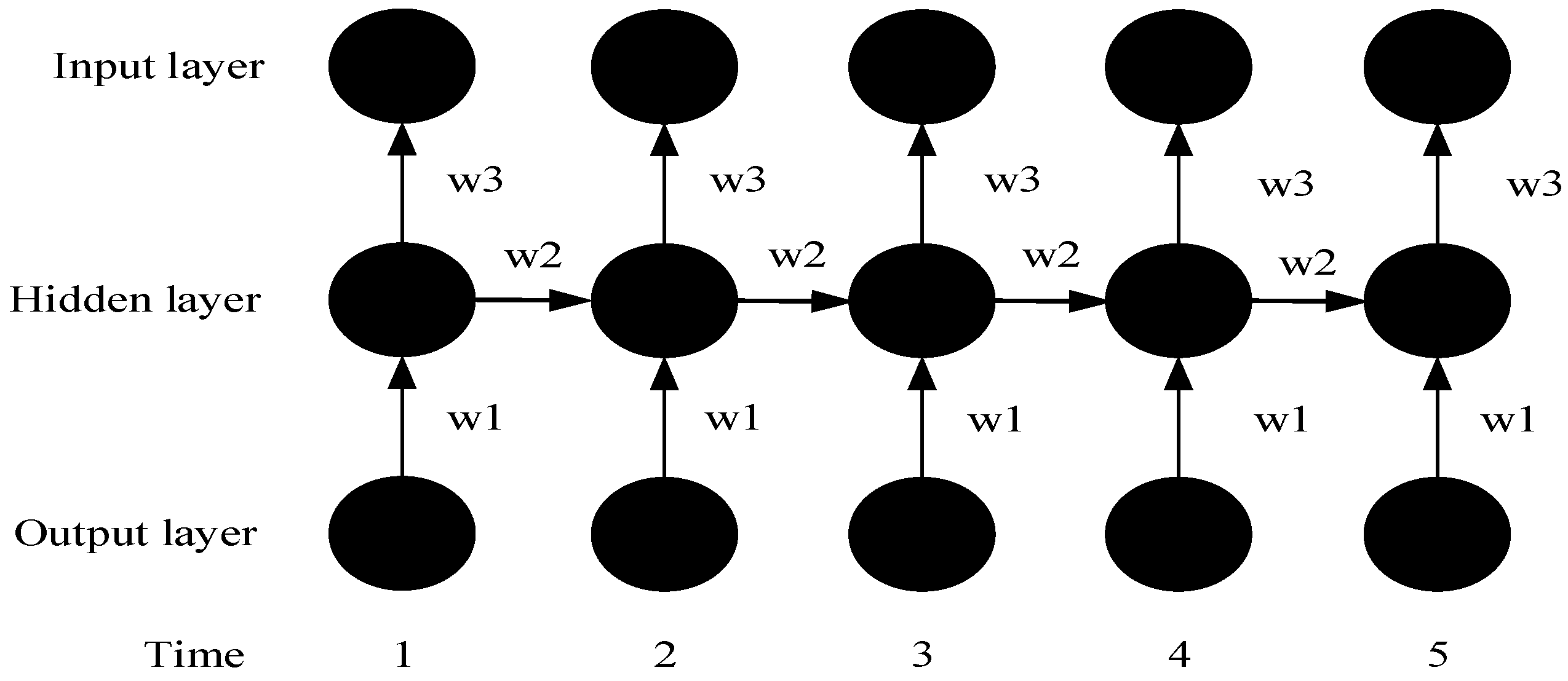
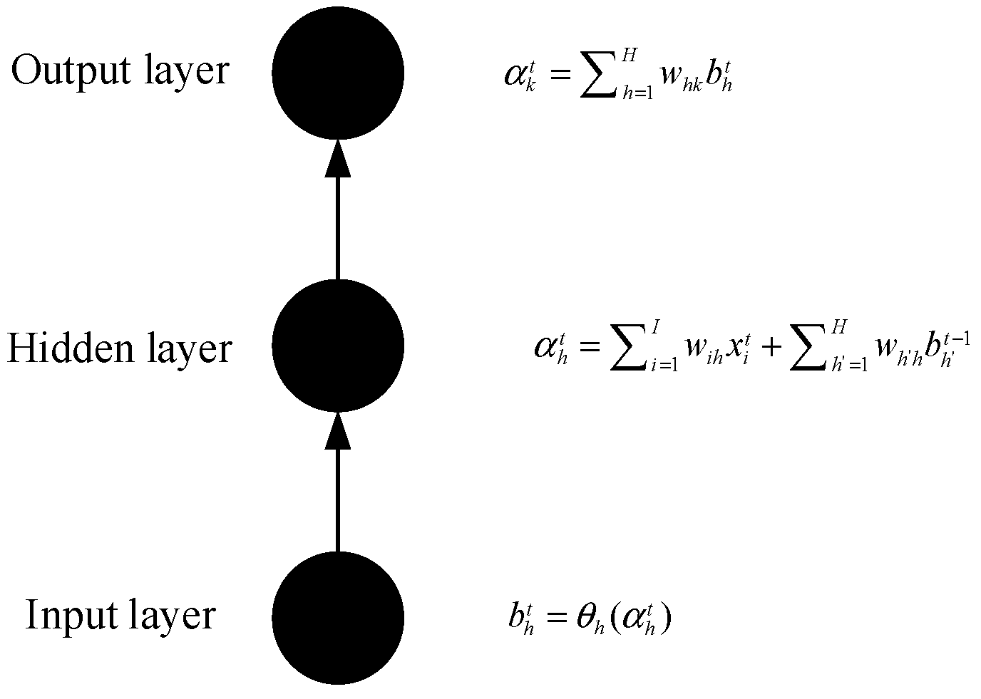
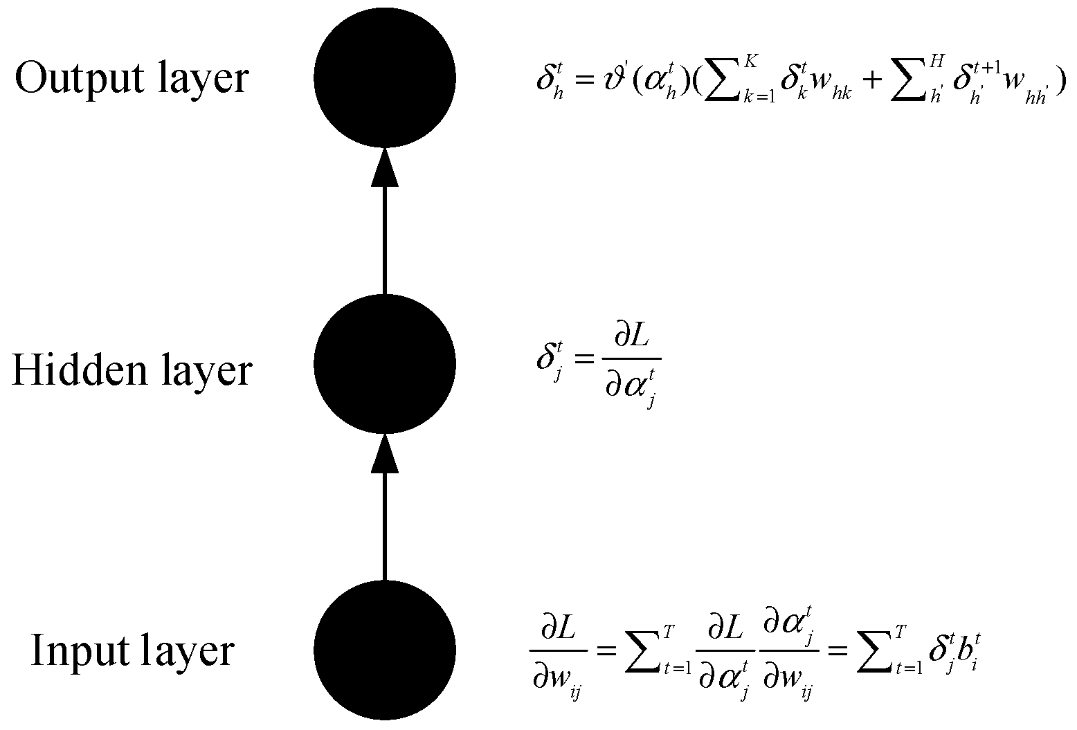
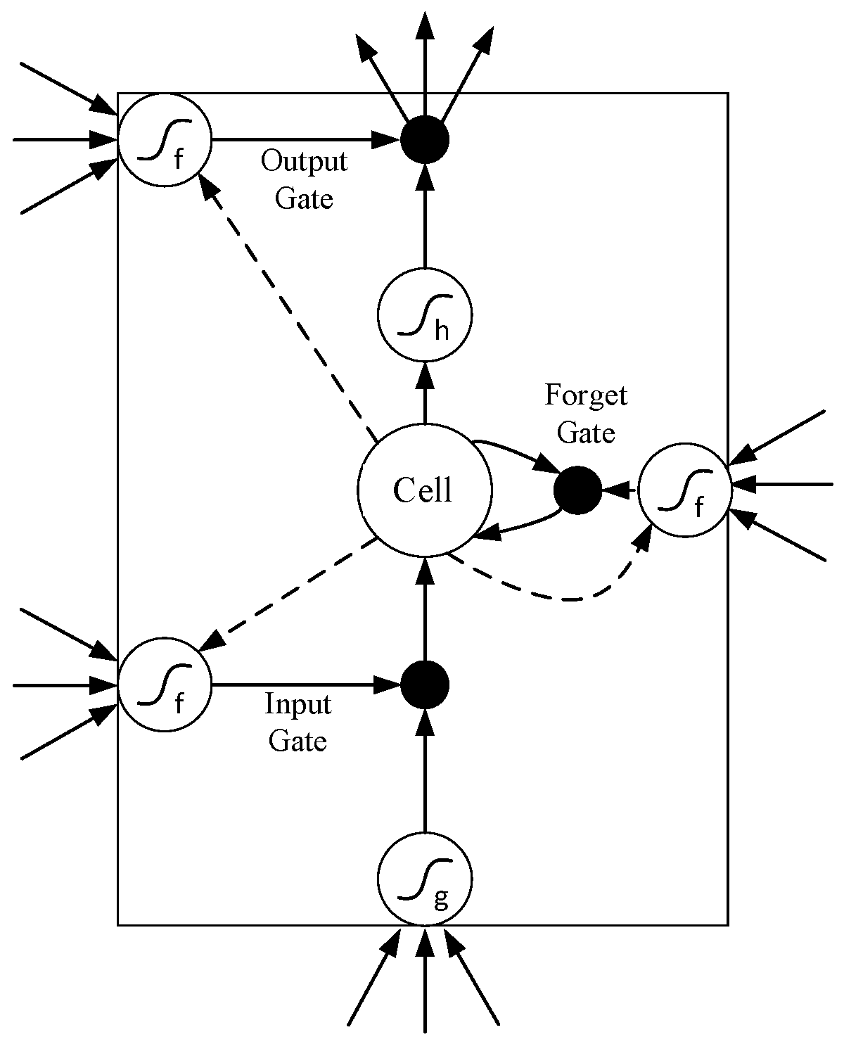
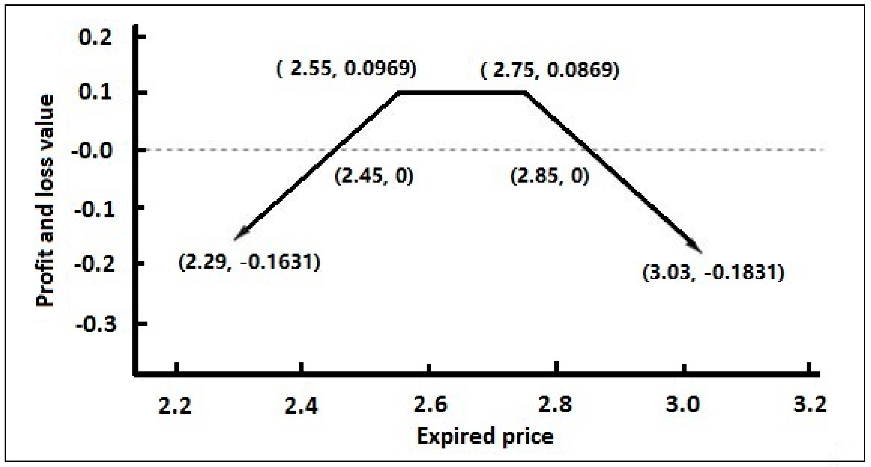
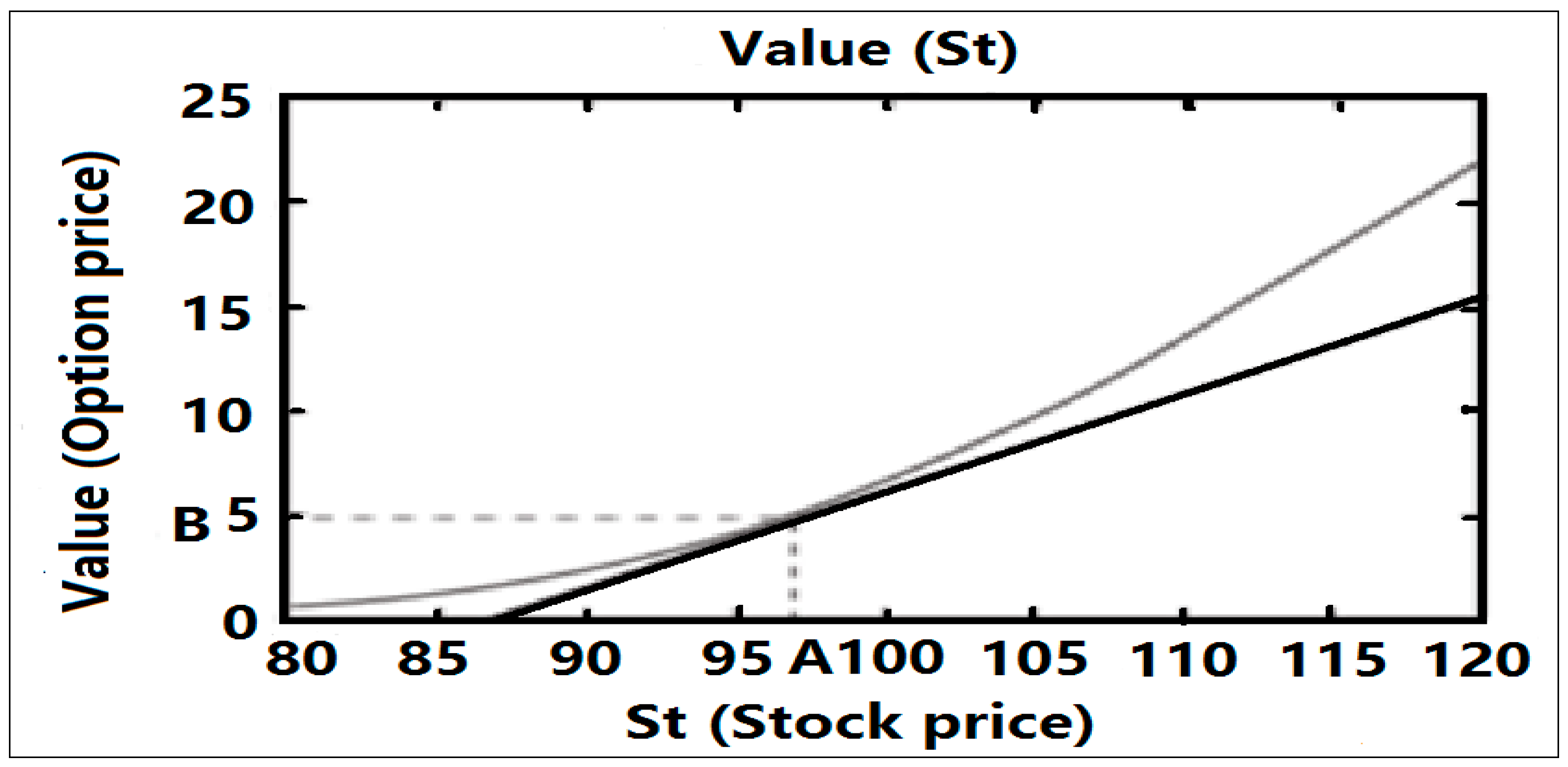
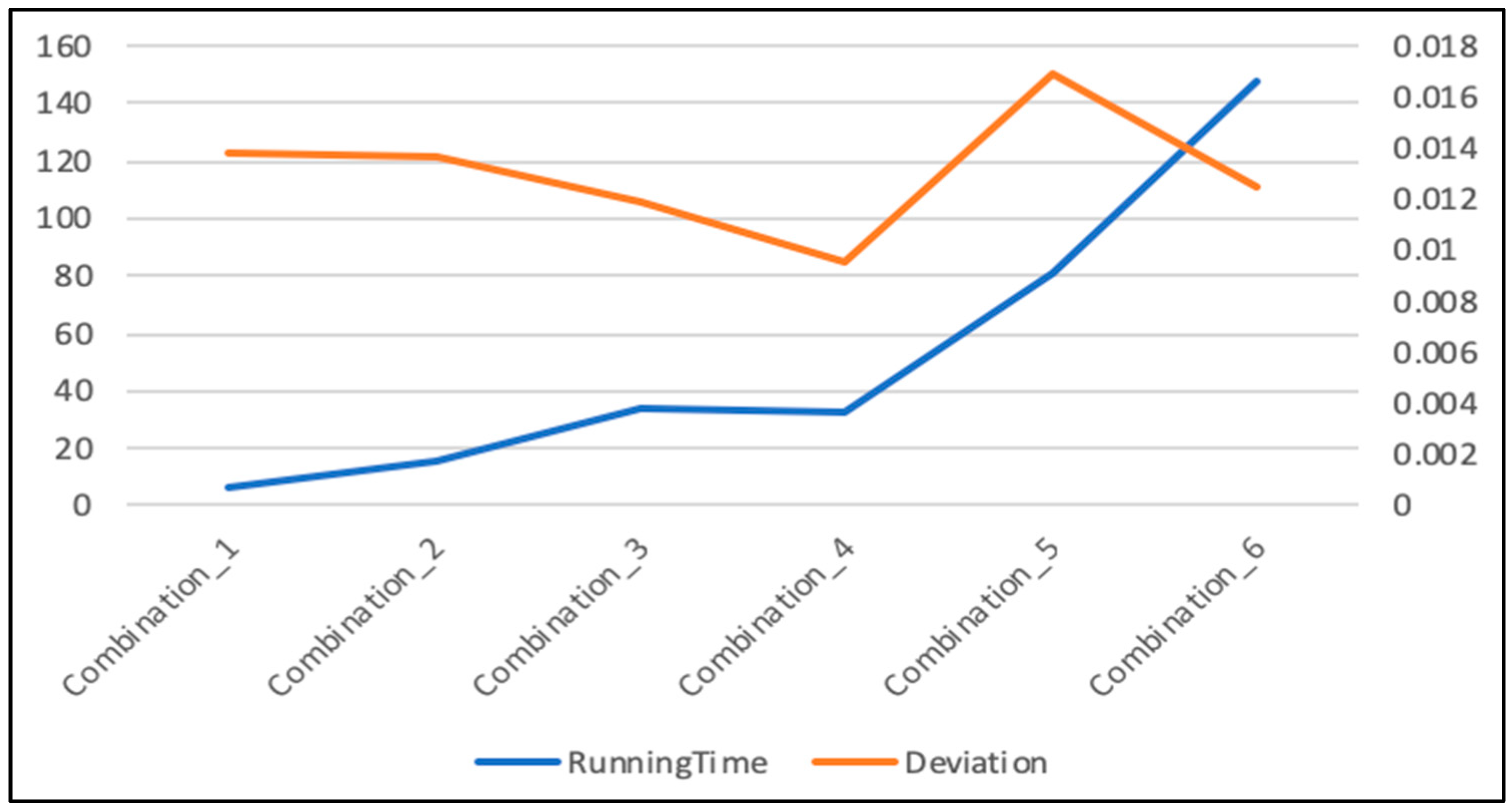
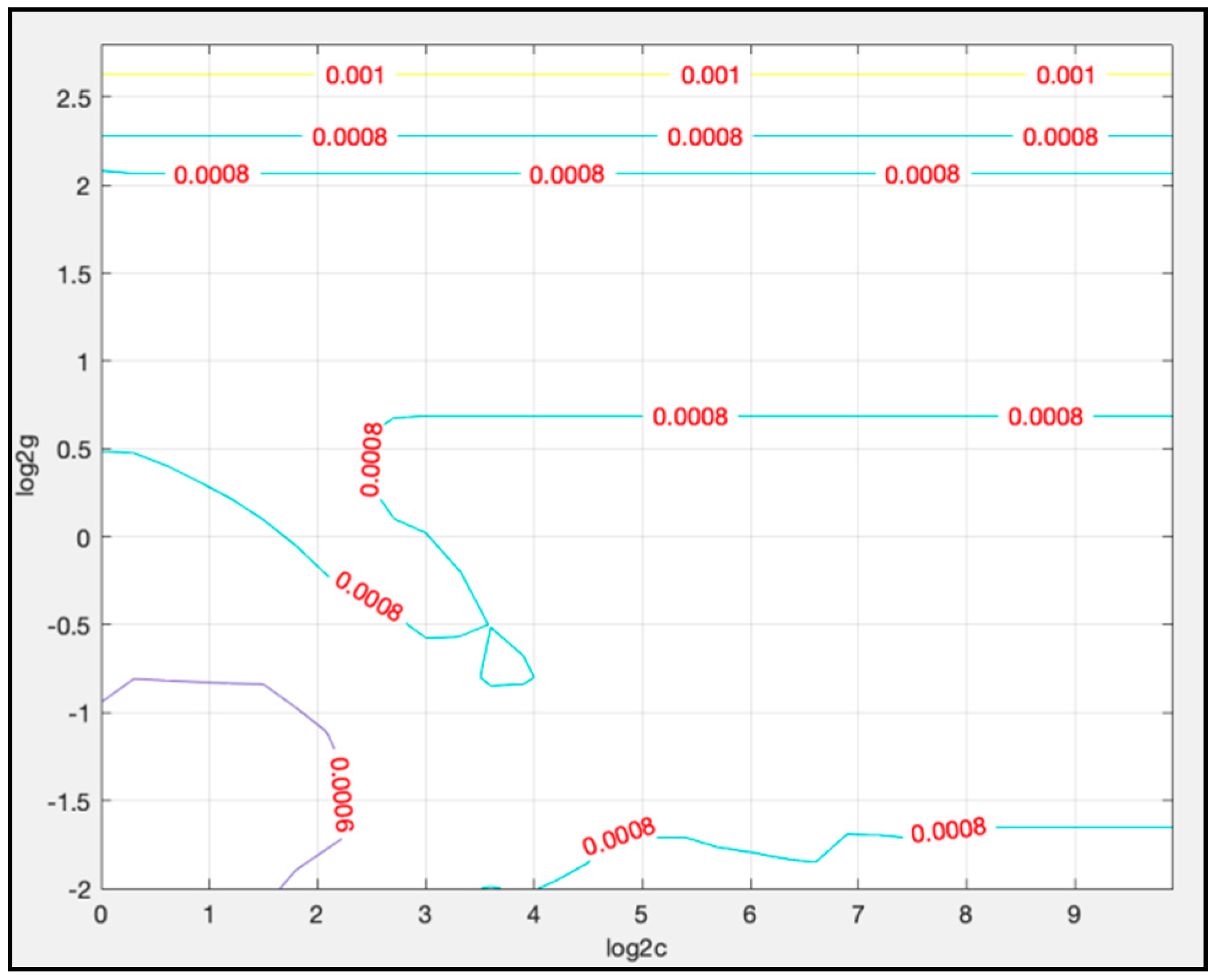
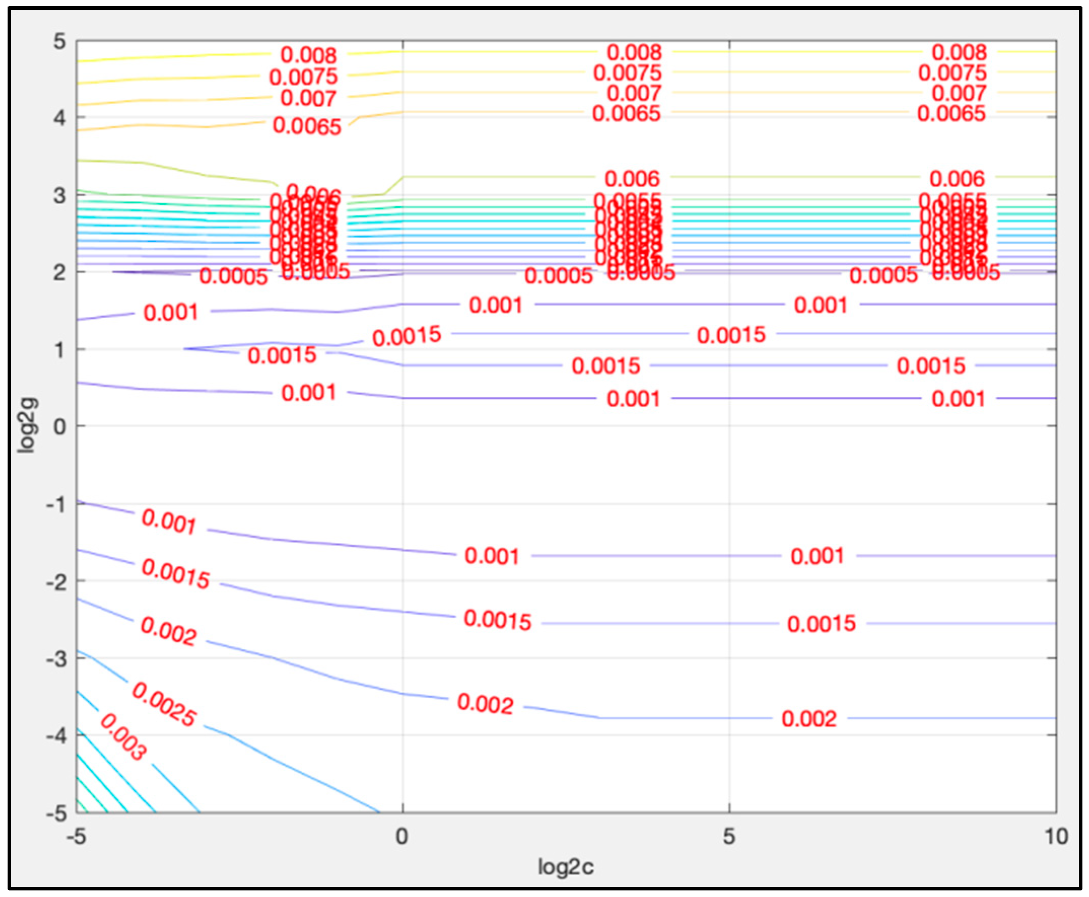
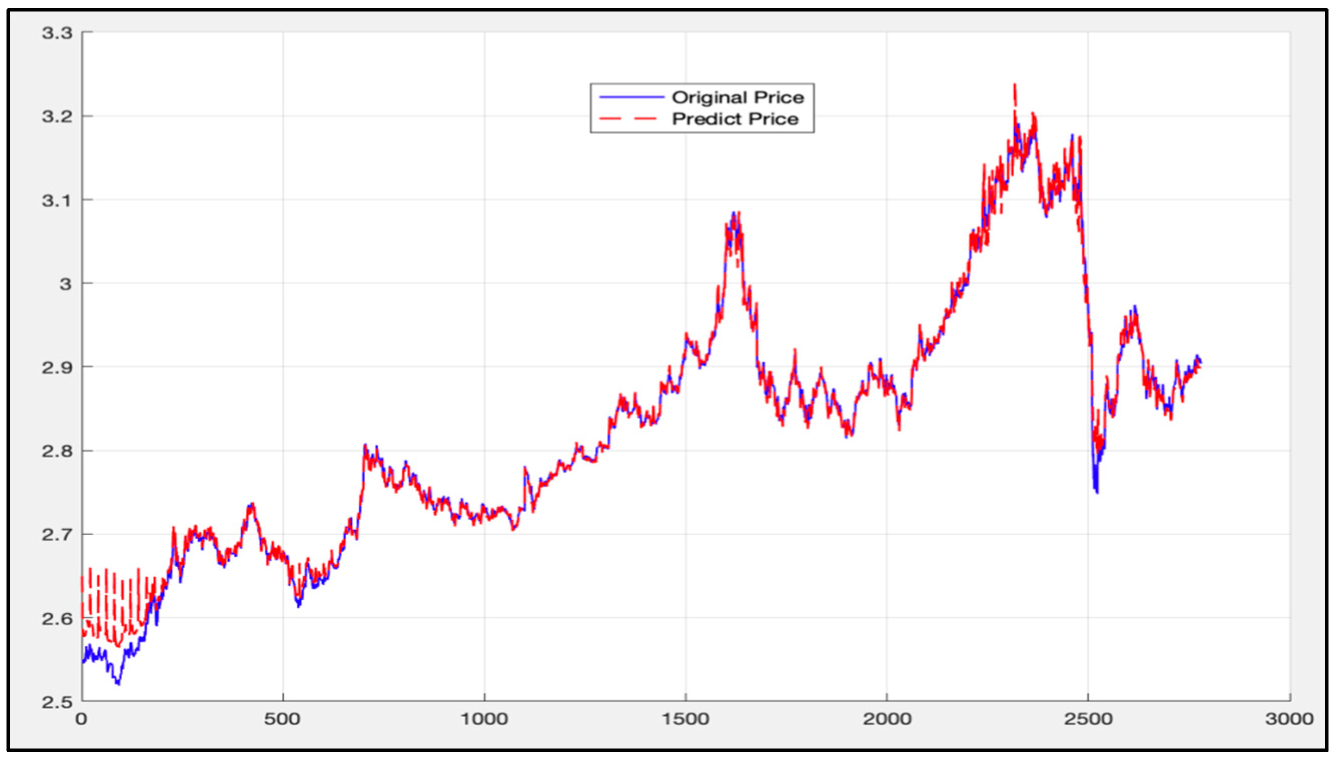
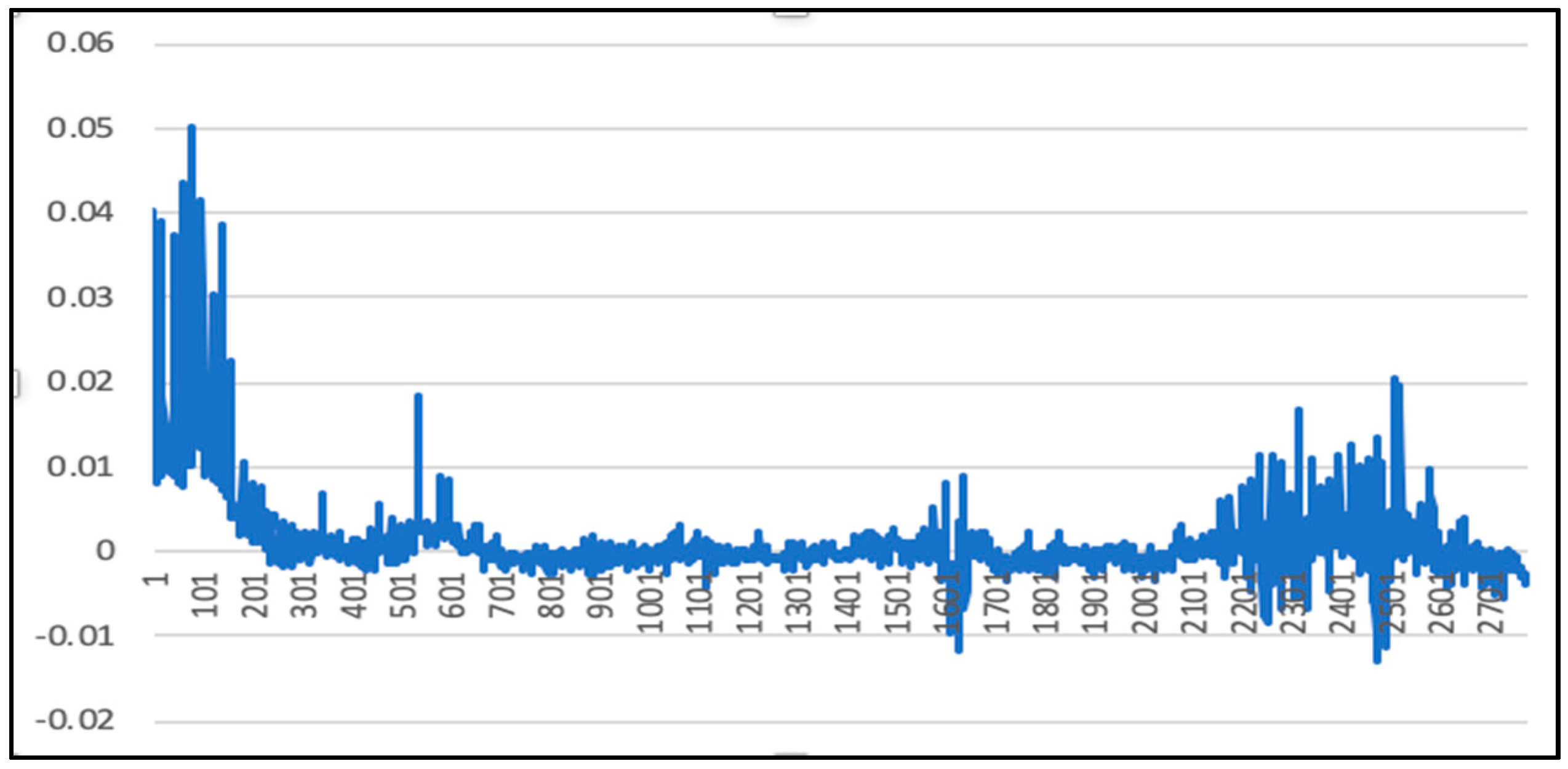
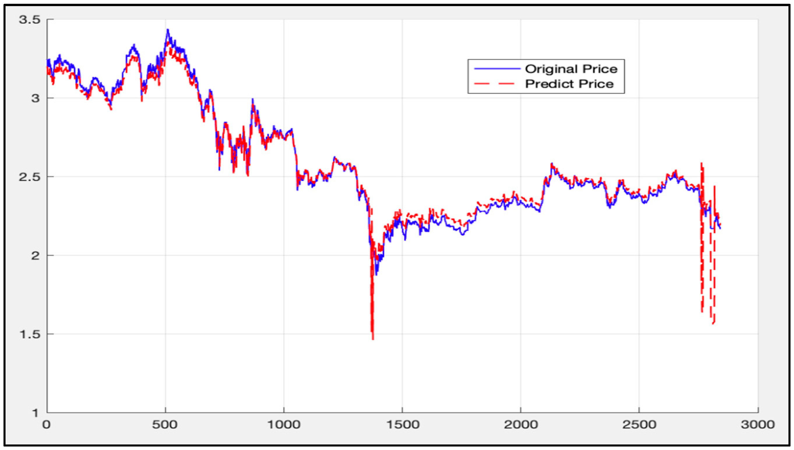
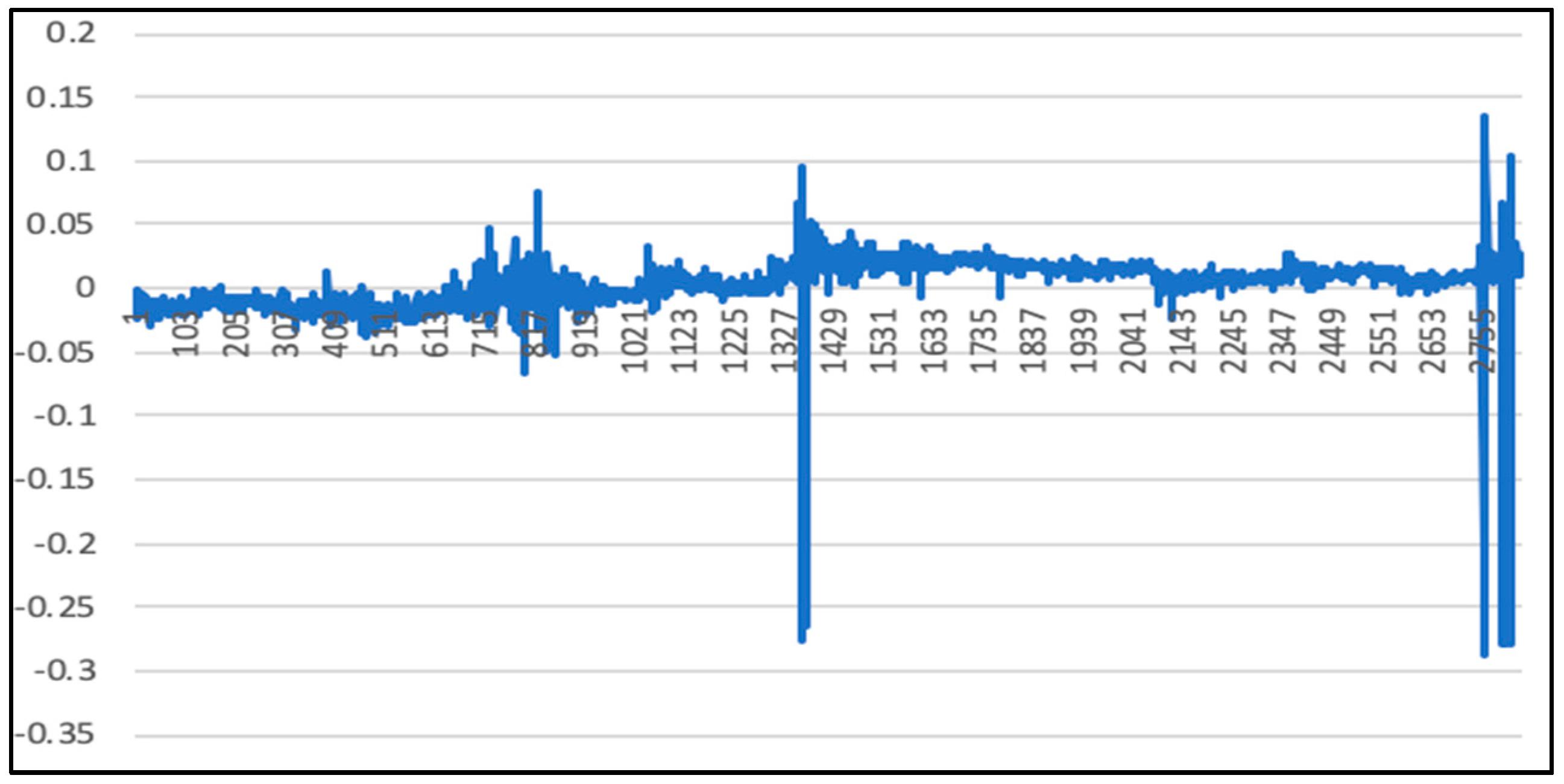
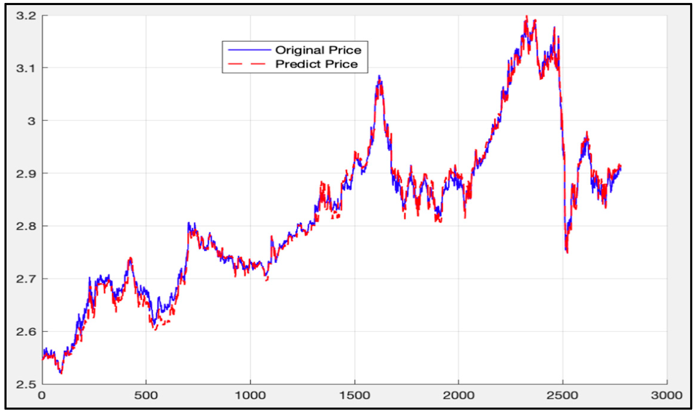
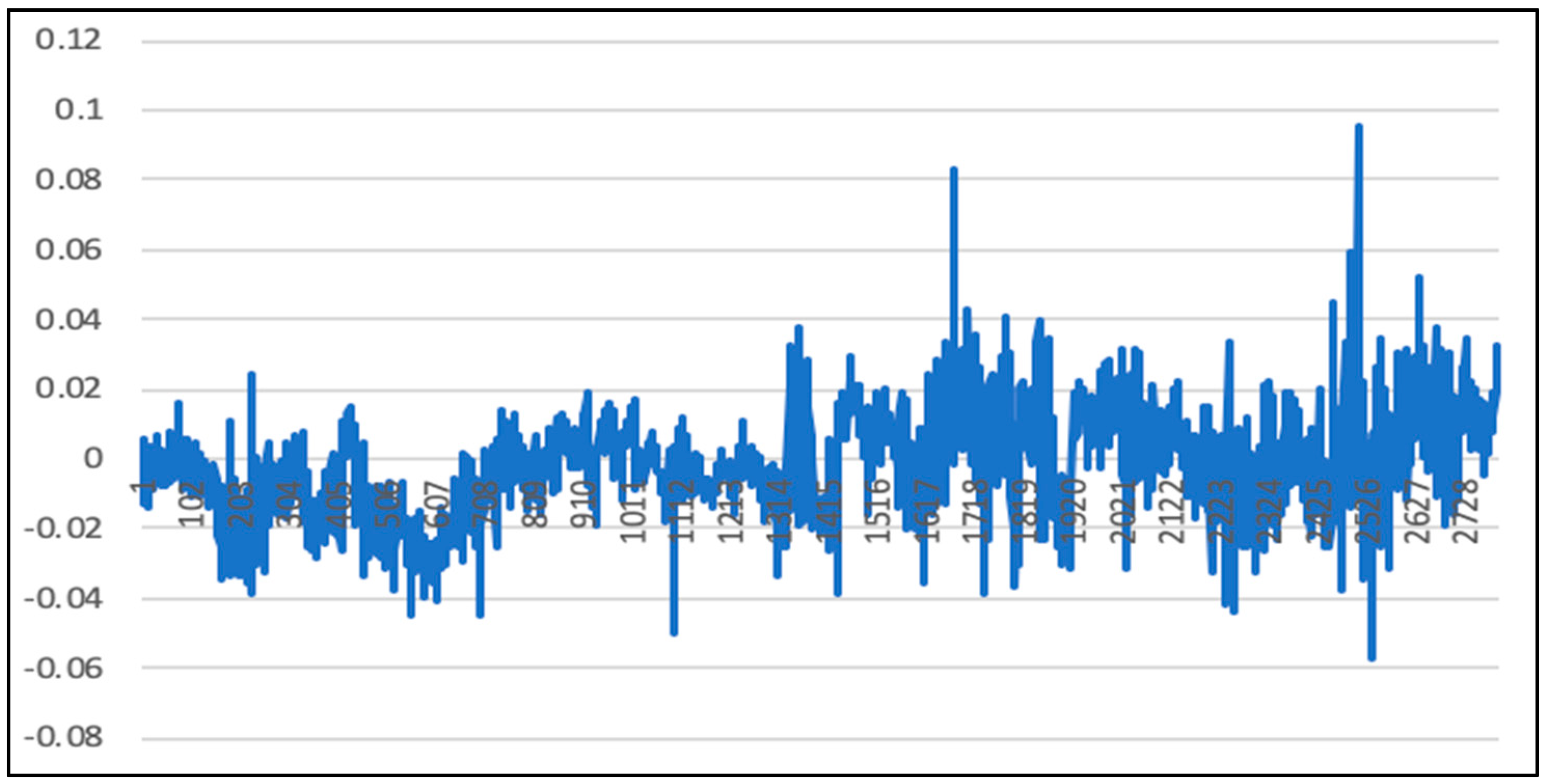
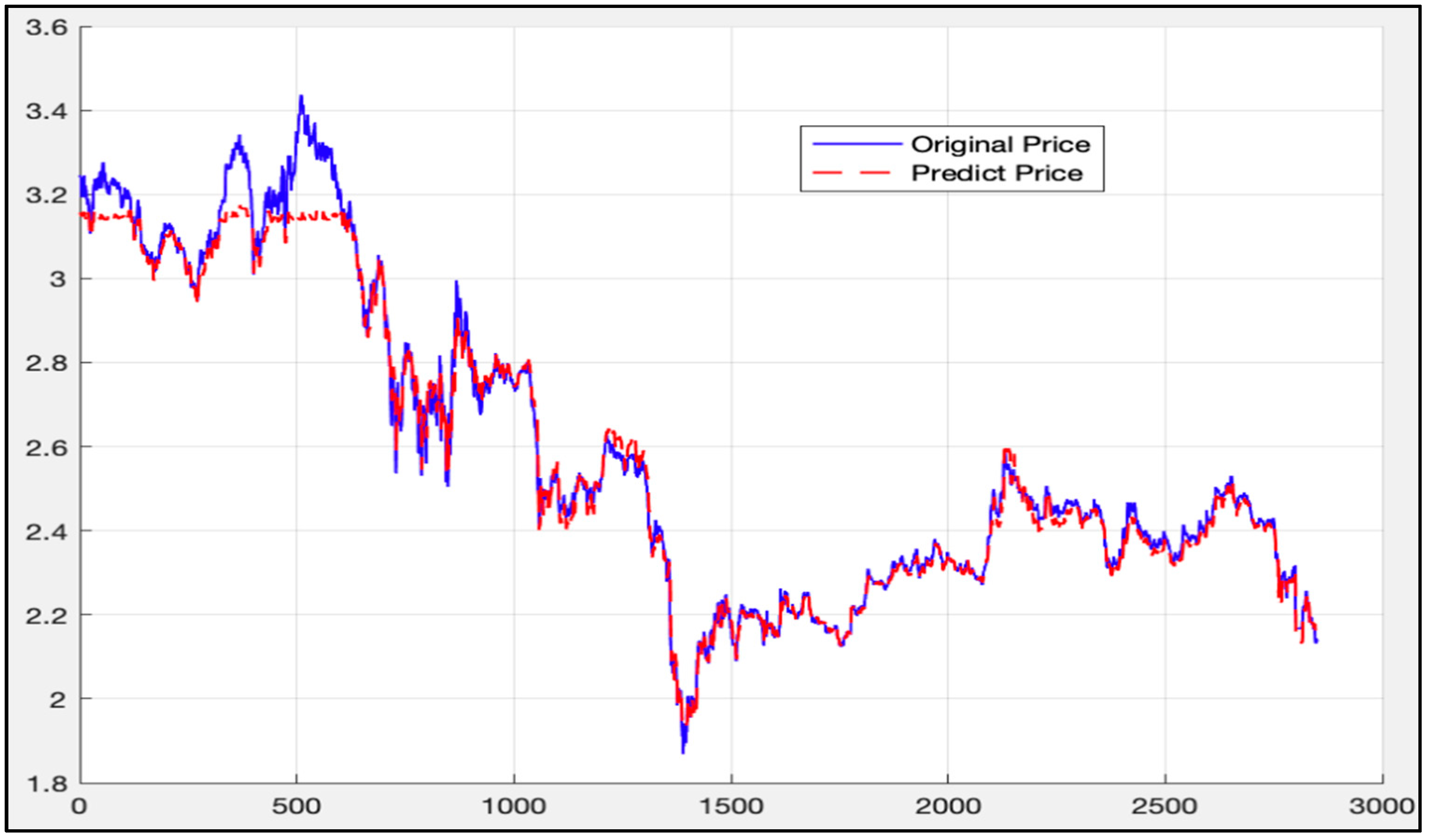
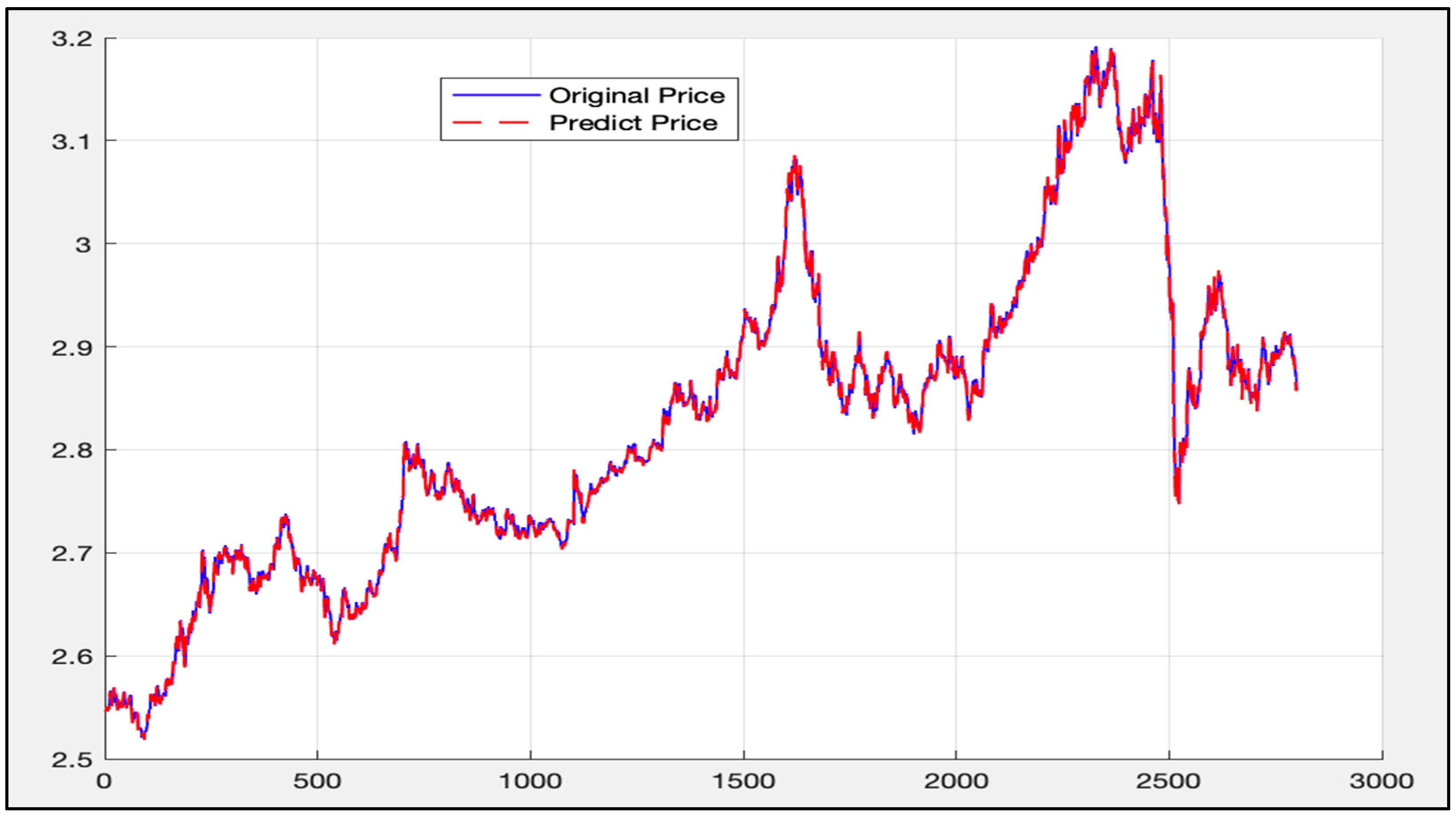
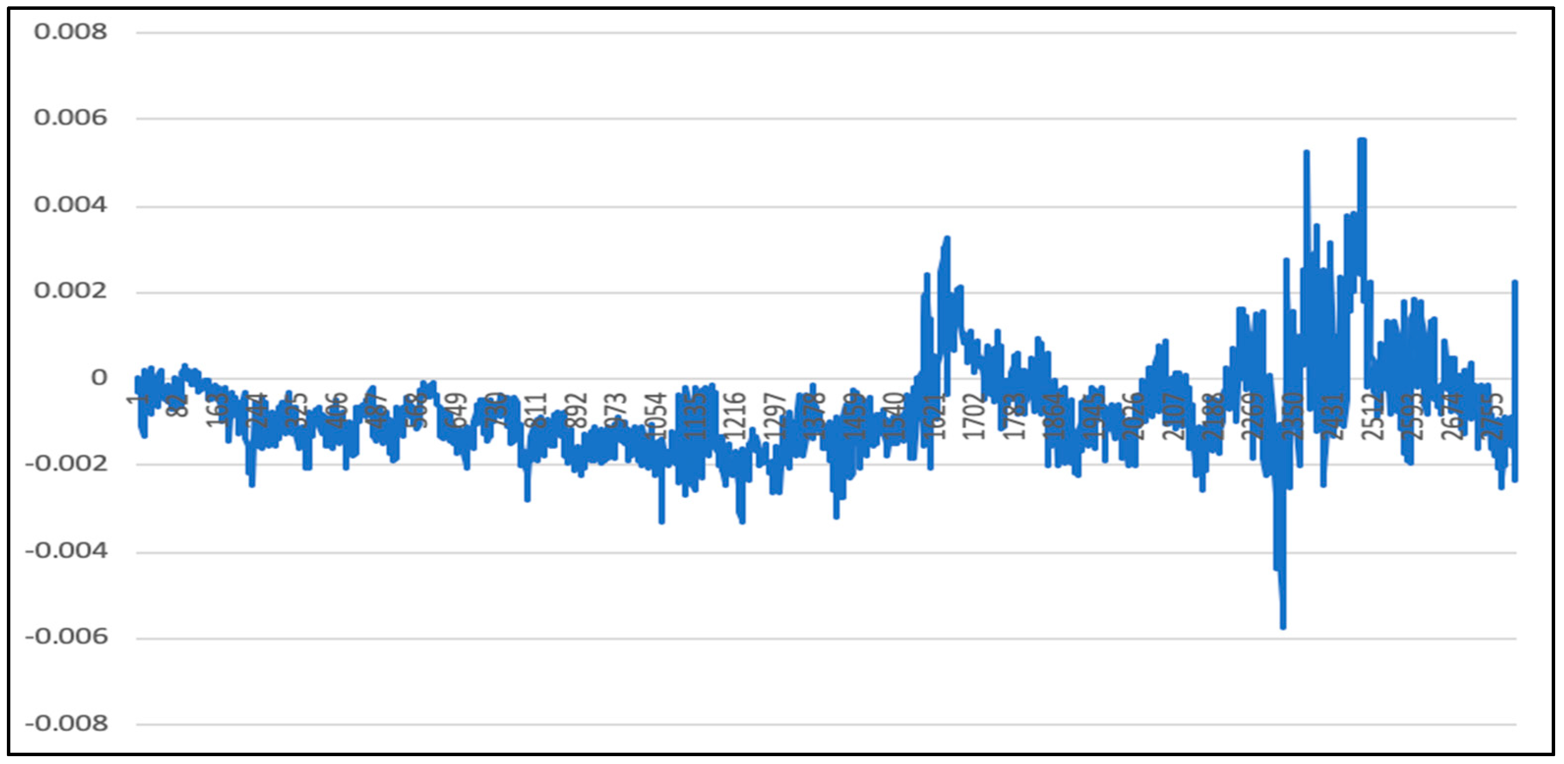
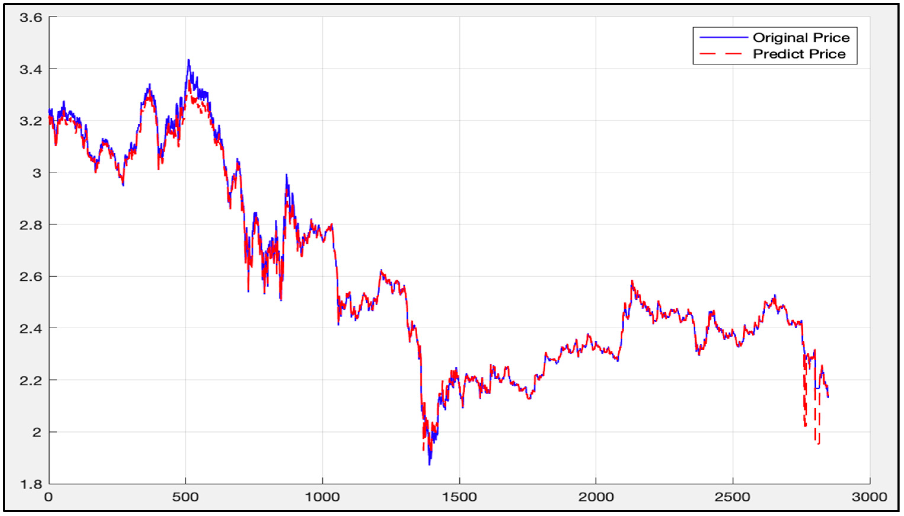
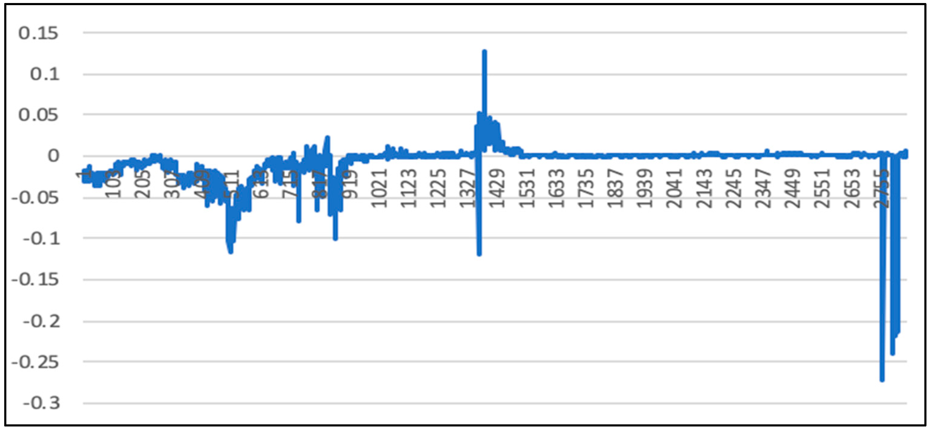
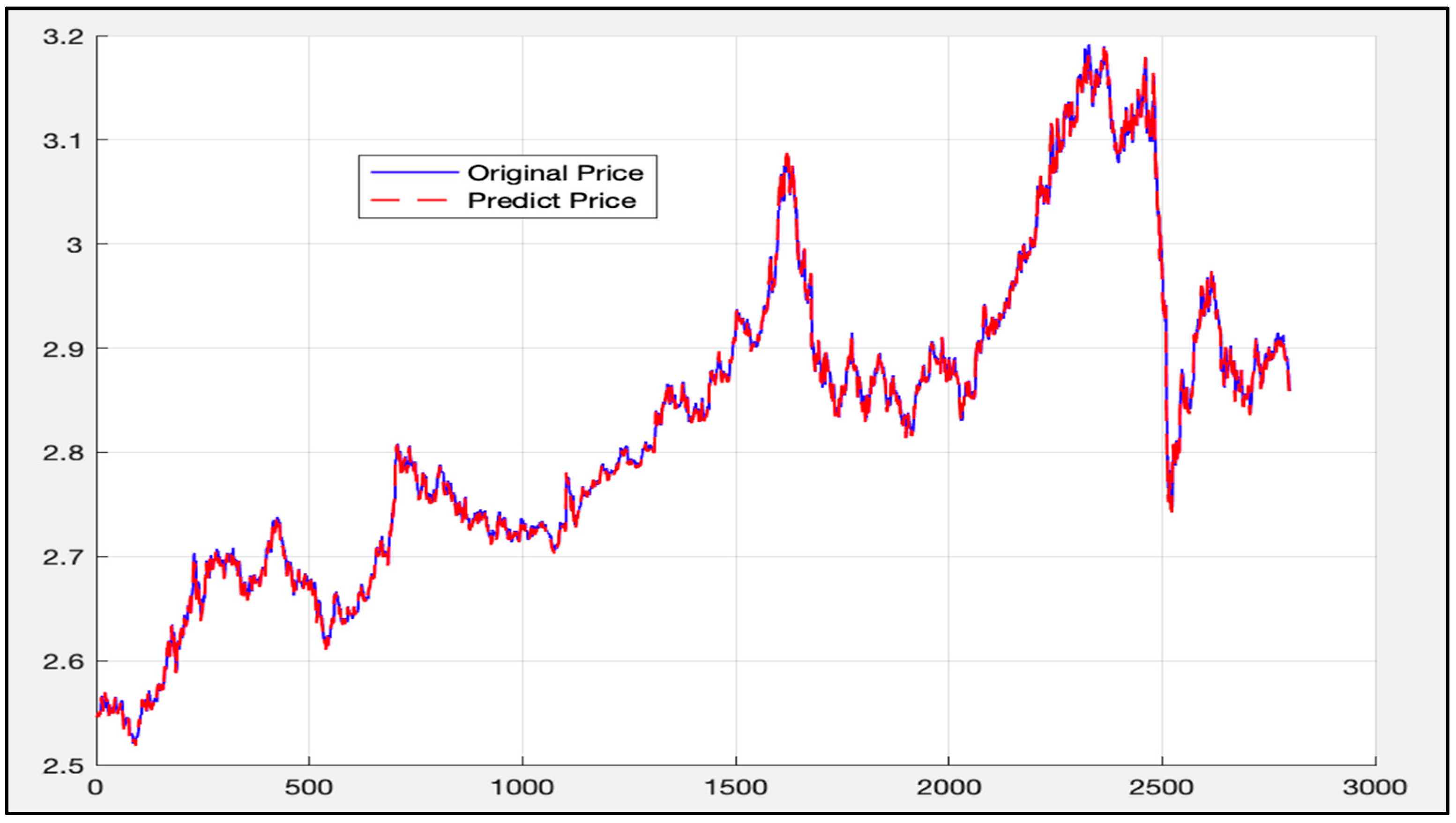
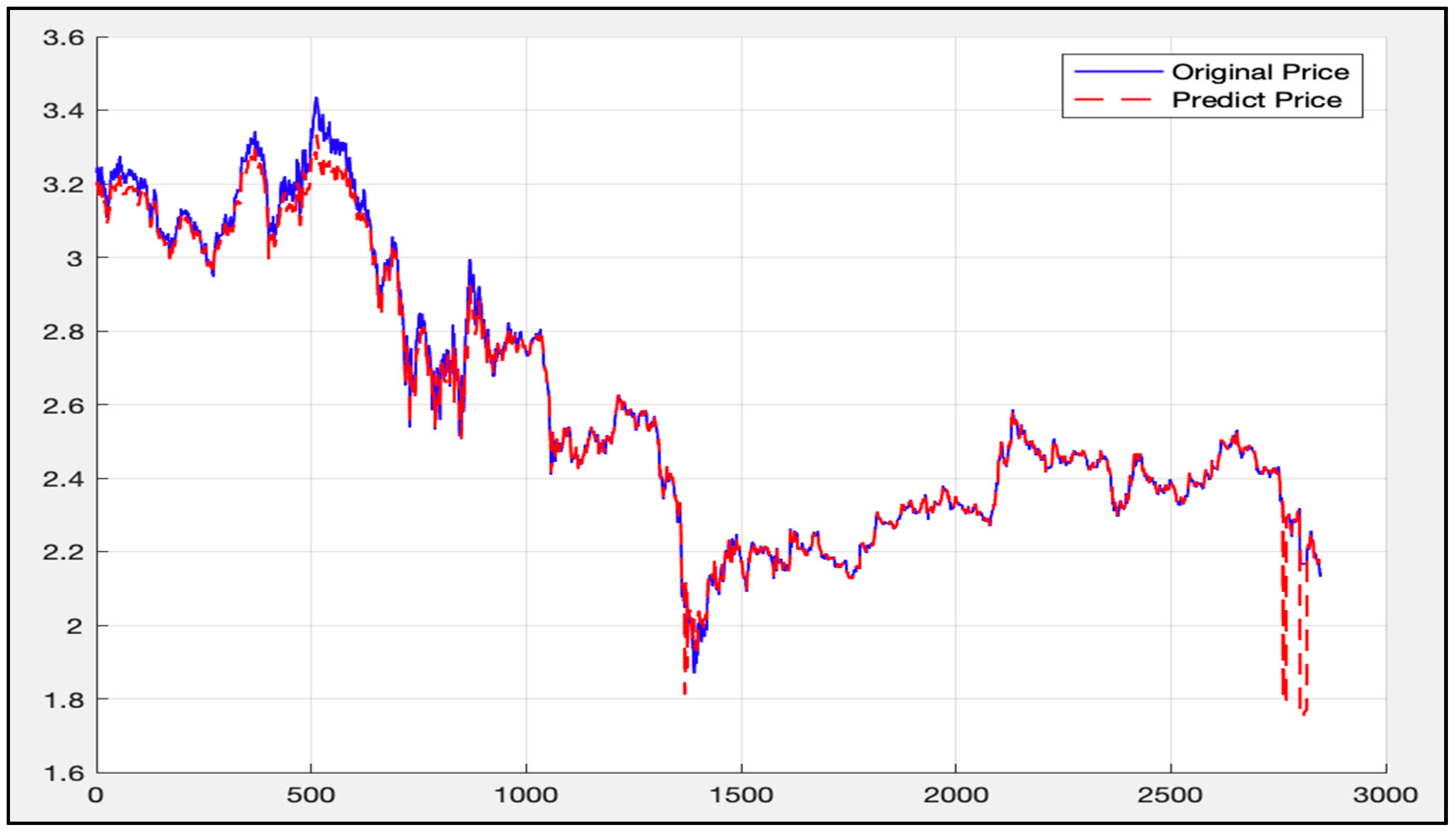
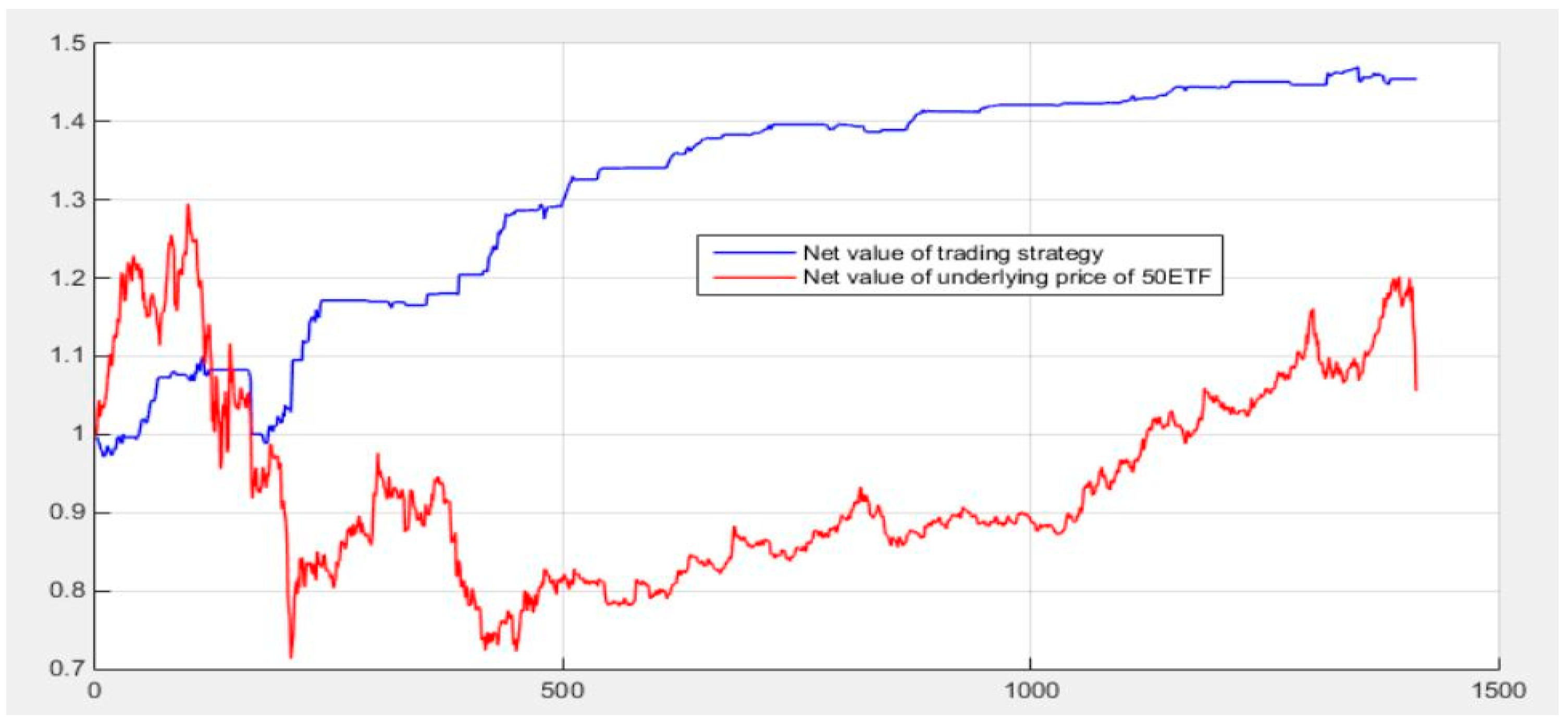
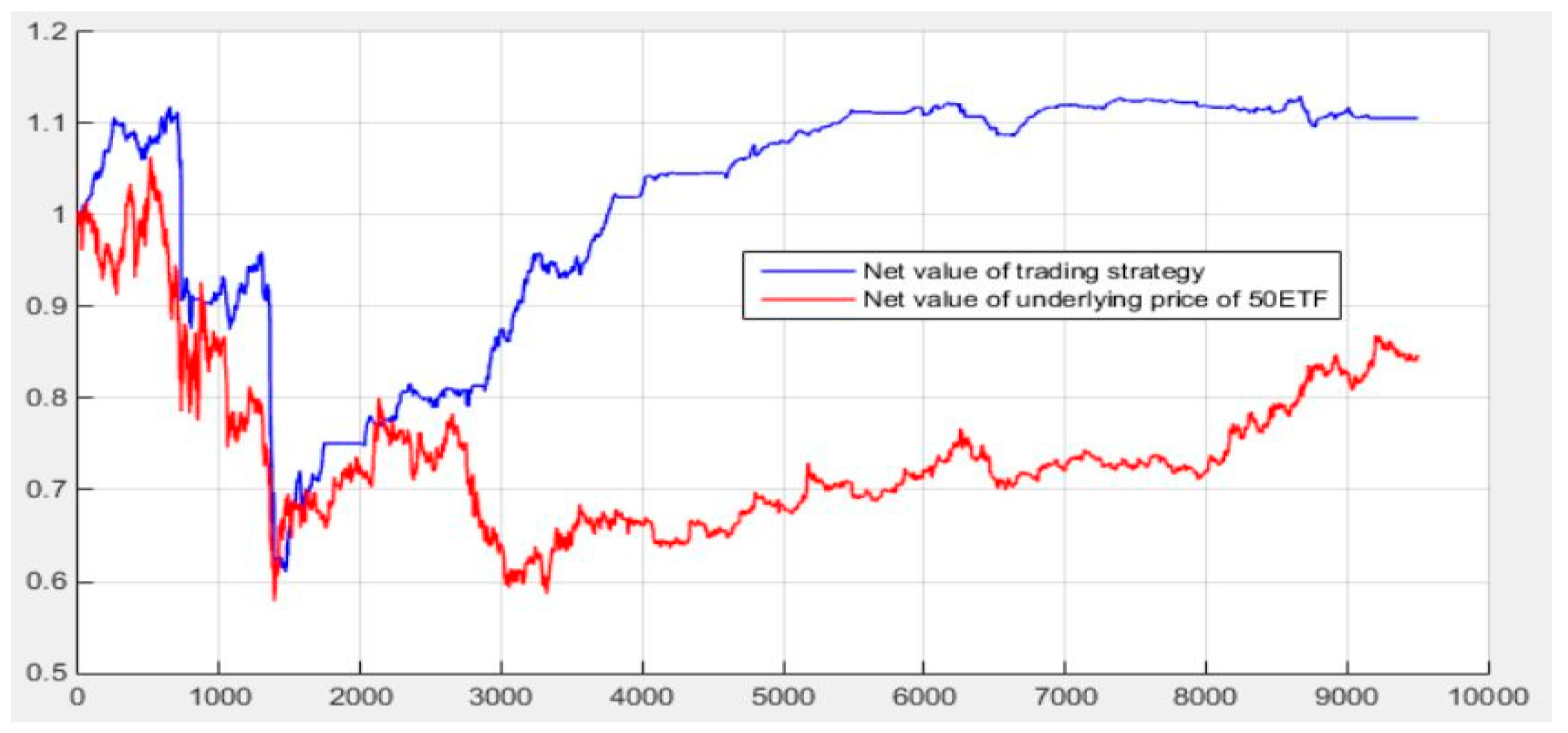
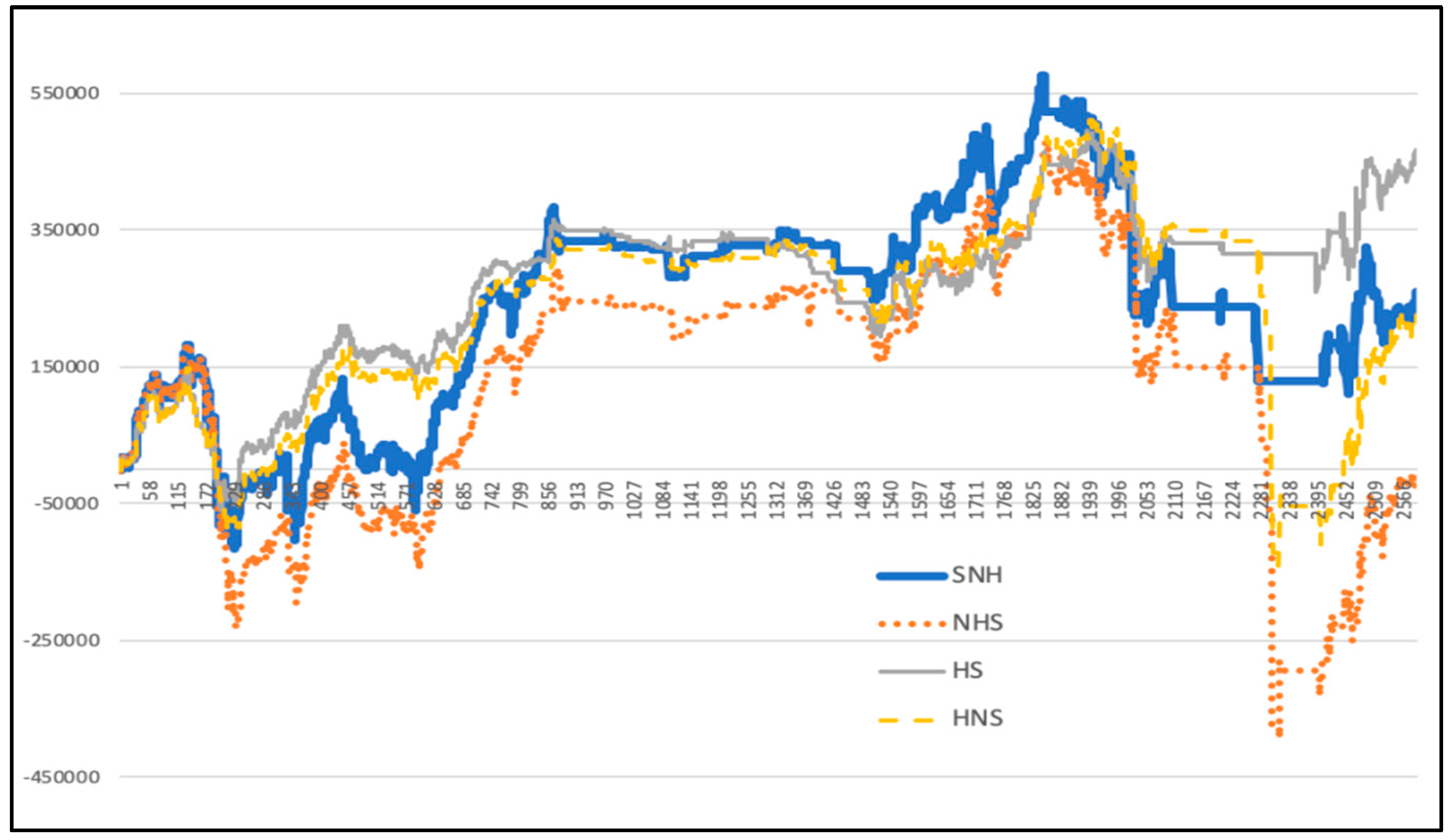
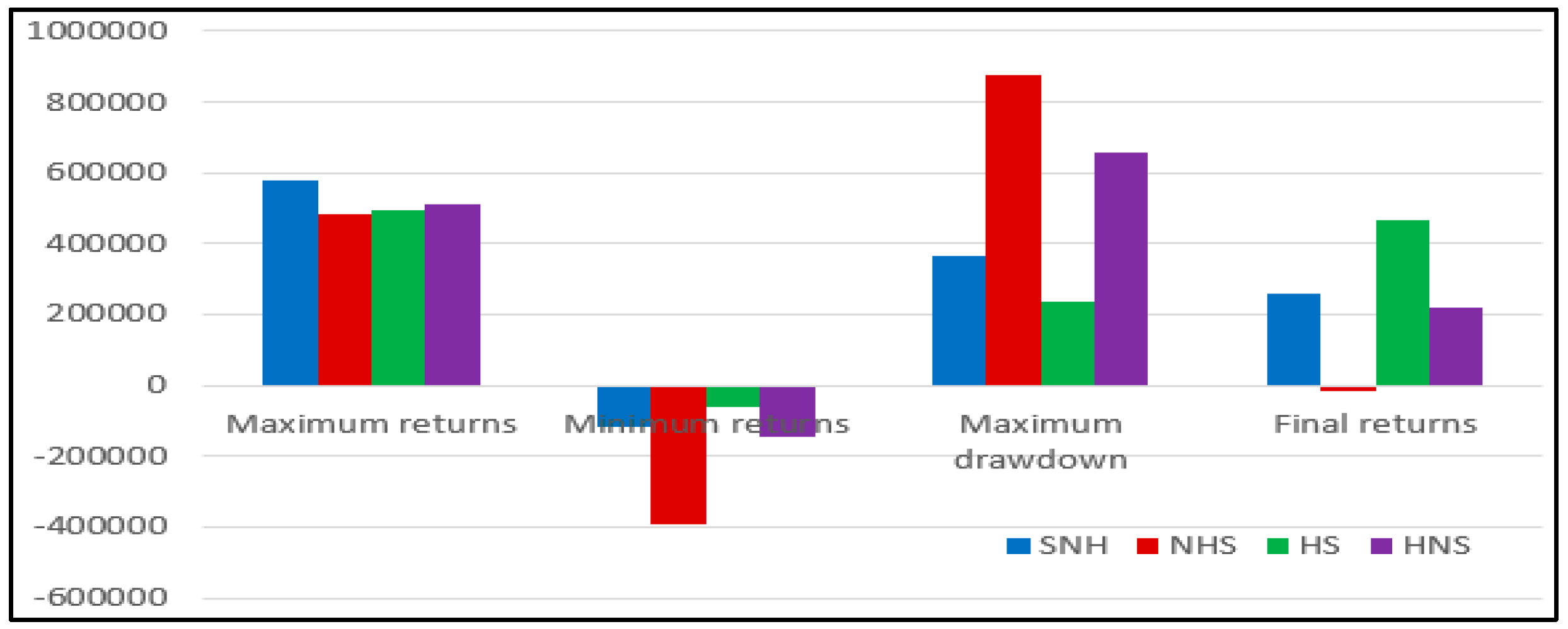
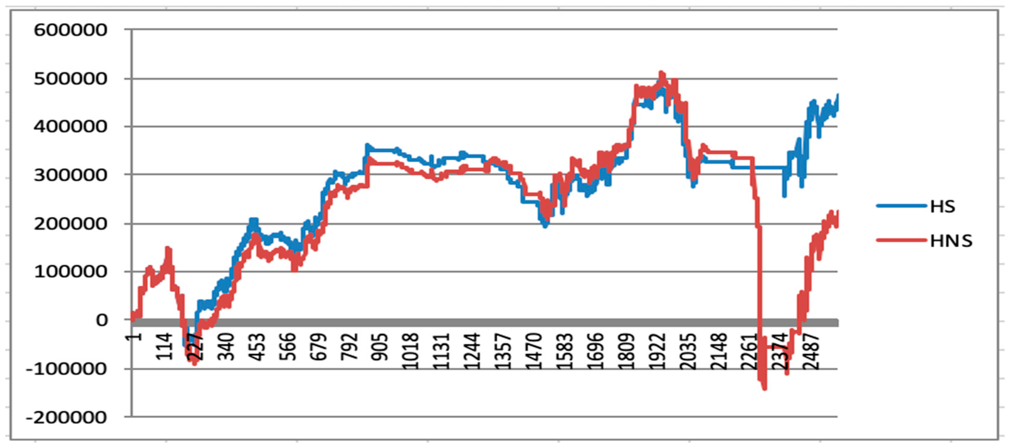
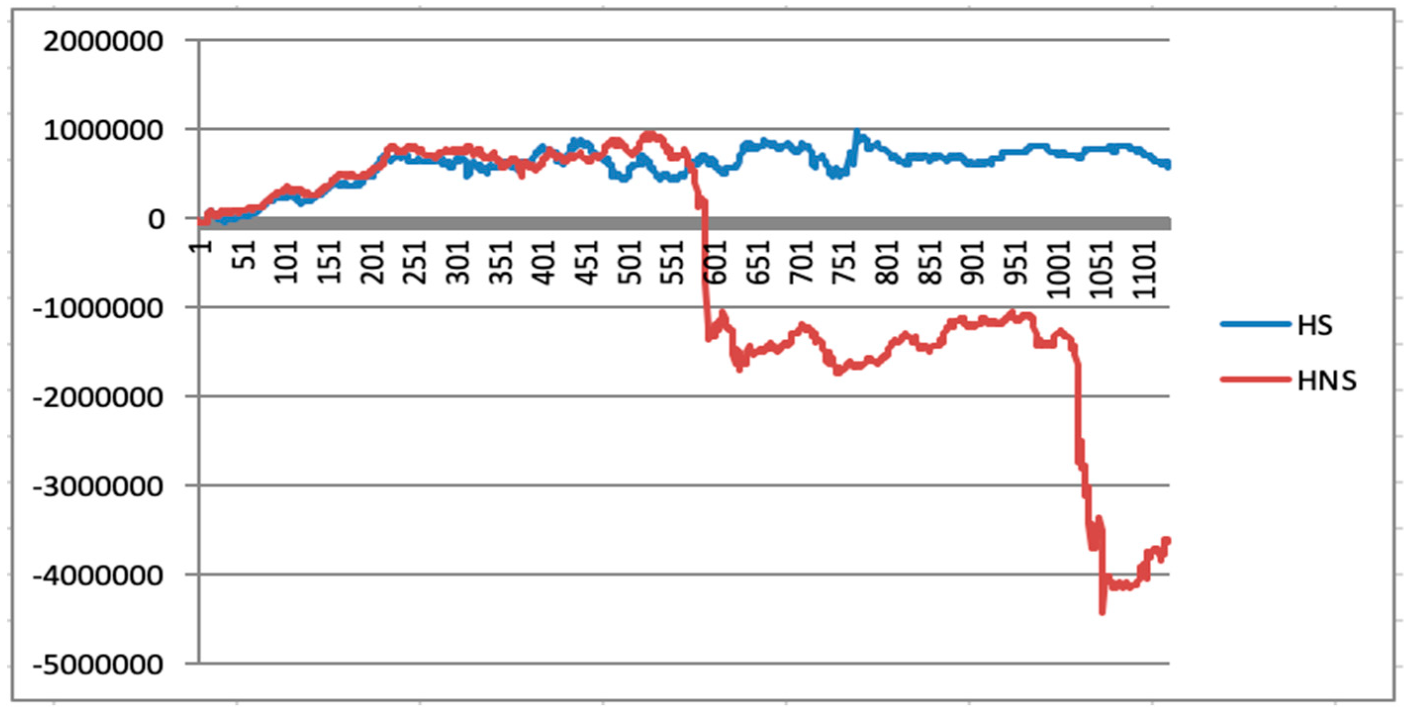
Table 1.
Example of a strangle options short-sell investment strategy.
| Subject Contract Name | Buy or Sell | Quantity | Options Price |
|---|---|---|---|
| 50 ETF buying December 2750 | Sell | 1 | 0.0635 |
| 50 ETF selling December 2550 | Sell | 1 | 0.0334 |
Table 2.
Results of six different situations.
| Hidden Units | Iteration Times | TimeStep | Batch_Size | Runningtime | Deviation |
|---|---|---|---|---|---|
| 20 | 200 | 16 | 80 | 6 min | 0.013833 |
| 20 | 1000 | 16 | 80 | 16 min | 0.013703 |
| 20 | 2000 | 16 | 80 | 34 min | 0.011918 |
| 20 | 2000 | 20 | 60 | 32 min | 0.009551 |
| 60 | 2000 | 16 | 80 | 1 h 21 min | 0.016878 |
| 100 | 2000 | 20 | 60 | 2 h 27 min | 0.012416 |
Table 3.
Final result of fine selection.
| Cross-validation mean squared error (MSE) | 0.00117032 |
| Cross-validation squared correlation coefficient | 0.987437 |
| Best cross-validation MSE | 0.000496649 |
| Best c | 1.23114 |
| Best g | 0.378929 |
Table 4.
Results of the fine selection.
| Cross-validation mean squared error | 0.00214727 |
| Cross-validation squared correlation coefficient | 0.980383 |
| Best cross-validation MSE | 0.000388862 |
| Best c | 1 |
| Best g | 0.466516 |
Table 5.
Comparison table of deviation values predicted by the LSTM model and the LSTM-SVR model over two time periods.
Table 5.
Comparison table of deviation values predicted by the LSTM model and the LSTM-SVR model over two time periods.
| LSTM (Deviation) | RF (Deviation) | |
|---|---|---|
| 20170628 (11:30) –20180314 (10:30) | 0.00232 | 0.00475 |
| 20150414 (10:30) –20160112 (13:45) | 0.00903 | 0.01189 |
Table 6.
Comparison table of the deviation values predicted by the LSTM-SVR I and LSTM-SVR II models (different input vectors) over two time periods.
Table 6.
Comparison table of the deviation values predicted by the LSTM-SVR I and LSTM-SVR II models (different input vectors) over two time periods.
| LSTM-SVR I (Deviation, Only Using Output) | LSTM-SVR II (Deviation, Using Hidden State Vector) | |
|---|---|---|
| 20170628(11:30) −20180314(10:30) | 0.00025 | 0.00062 |
| 20150414(10:30) −20160112(13:45) | 0.0023 | 0.00552 |
Table 7.
Comparison of four strategic situations.
| SNH | NHS | HS | HNS | |
|---|---|---|---|---|
| Maximum returns | 576,767.6 | 484,294 | 493,478.8 | 511,736.6 |
| Minimum returns | −116,804.2 | −393,156.8 | −61,717.6 | −143,753.8 |
| Maximum drawdown | 362,872.8 | 877,450.8 | 2,352,84.4 | 655,490.4 |
| Final returns | 258,675.6 | −15,720.4 | 464,496 | 219,288. |
© 2019 by the authors. Licensee MDPI, Basel, Switzerland. This article is an open access article distributed under the terms and conditions of the Creative Commons Attribution (CC BY) license (http://creativecommons.org/licenses/by/4.0/).
Share and Cite
MDPI and ACS Style
Fang, Y.; Chen, J.; Xue, Z. Research on Quantitative Investment Strategies Based on Deep Learning. Algorithms 2019, 12, 35. https://0-doi-org.brum.beds.ac.uk/10.3390/a12020035
AMA Style
Fang Y, Chen J, Xue Z. Research on Quantitative Investment Strategies Based on Deep Learning. Algorithms. 2019; 12(2):35. https://0-doi-org.brum.beds.ac.uk/10.3390/a12020035
Chicago/Turabian StyleFang, Yujie, Juan Chen, and Zhengxuan Xue. 2019. "Research on Quantitative Investment Strategies Based on Deep Learning" Algorithms 12, no. 2: 35. https://0-doi-org.brum.beds.ac.uk/10.3390/a12020035
Note that from the first issue of 2016, this journal uses article numbers instead of page numbers. See further details here.