A Heuristic Approach for a Real-World Electric Vehicle Routing Problem


1
School of Automobile and Traffic Engineering, Wuhan University of Science and Technology, Wuhan 430065, China
2
School of Mechanical Engineering, Guangxi University of Science and Technology, Liuzhou 545006, China
*
Author to whom correspondence should be addressed.
Algorithms 2019, 12(2), 45; https://0-doi-org.brum.beds.ac.uk/10.3390/a12020045
Submission received: 8 January 2019
/
Revised: 12 February 2019
/
Accepted: 13 February 2019
/
Published: 20 February 2019
Abstract
:To develop a non-polluting and sustainable city, urban administrators encourage logistics companies to use electric vehicles instead of conventional (i.e., fuel-based) vehicles for transportation services. However, electric energy-based limitations pose a new challenge in designing reasonable visiting routes that are essential for the daily operations of companies. Therefore, this paper investigates a real-world electric vehicle routing problem (VRP) raised by a logistics company. The problem combines the features of the capacitated VRP, the VRP with time windows, the heterogeneous fleet VRP, the multi-trip VRP, and the electric VRP with charging stations. To solve such a complicated problem, a heuristic approach based on the adaptive large neighborhood search (ALNS) and integer programming is proposed in this paper. Specifically, a charging station adjustment heuristic and a departure time adjustment heuristic are devised to decrease the total operational cost. Furthermore, the best solution obtained by the ALNS is improved by integer programming. Twenty instances generated from real-world data were used to validate the effectiveness of the proposed algorithm. The results demonstrate that using our algorithm can save 7.52% of operational cost.
1. Introduction
With industrial development and urbanization, air pollution in cities has become increasingly serious in recent years. For example, in December 2016, Beijing was covered by smog for six days, forcing authorities to announce the highest-level smog alert of 2016. A major cause of air pollution in cities is the large number of conventional motor vehicles with internal combustion engines that run on diesel or gasoline. They emit carbon oxides, nitrogen oxides and particulate matters that cause air pollution. To alleviate this hazardous situation and to reduce the number of conventional vehicles, green vehicles, such as alternative fuel vehicles and electric vehicles, which produce fewer emissions that contribute to air pollution than conventional vehicles, have gained much attention from city managers. Logistics companies are encouraged by city managers to use electric vehicles to construct a non-polluting and sustainable urban logistics system. For example, in January 2018, one of the largest Chinese online retailers, JD.com, used electric vehicles instead of conventional vehicles to deliver parcels in Beijing, and is going to replace all its conventional vehicles in the next two years. Electric vehicles are constrained by the capacity of their battery, the location of charging stations, and long charging times. The routing approaches for conventional vehicles are not applicable to electric vehicles, which leads to a new optimization problem called the electric vehicle routing problem (EVRP).
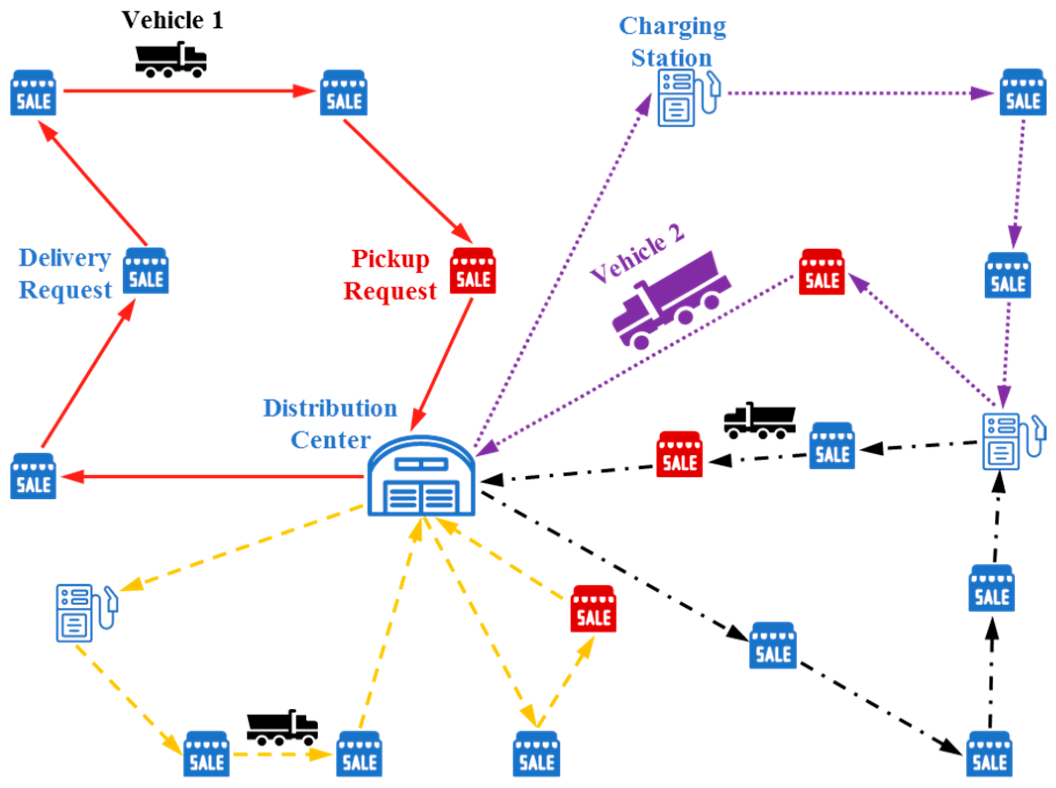
The basic EVRP is to obtain a set of routes with the minimum operational cost that serve customers’ requests while satisfying the driving range limitations and charging requirements of electric vehicles. A real-world EVRP proposed by a logistics company in Wuhan, China is presented in this paper. In the problem, a fleet of heterogeneous electric vehicles departs from the distribution center, delivers or picks up customer parcels within predefined time windows, and finishes at the center. While in transit, a vehicle can return to the center to load parcels to be delivered or unload collected parcels, and it can also go to charging stations as well as the distribution center to fully charge its battery in a fixed time (e.g., 30 min). The objective is to minimize the sum of the acquisition costs of used vehicles, the travel costs of vehicles, the waiting costs at customers and centers, and the charging costs. In Figure 1, two types of electric vehicles, i.e., Vehicle 1 and Vehicle 2, are used to fulfill delivery or pickup requests of customers; the lines having the same color denote a visiting route of a vehicle in the day. The red route does not need to charge; the purple route requires two charges at two different stations, one of which it shares with the black route; and the yellow route with two trips needs to go back to the distribution center. Obviously, the problem combines the features of the capacitated VRP [1], the VRP with time windows [2,3], the heterogeneous fleet VRP [4], the multi-trip VRP [5], and the EVRP with charging stations [6]. Considering its complexity, we must resort to meta-heuristics to efficiently solve the proposed problem.
This paper focuses on developing a heuristic approach based on the adaptive large neighborhood search (ALNS) and integer programming (IP) to solve the proposed problem. In the algorithm, we devise a charging station adjustment heuristic based on labeling algorithm to obtain the optimal selection and location of charging stations in a given sequence of customers and a departure time adjustment heuristic to calculate the optimal departure time when vehicles should first leave from the distribution center. After the termination of the ALNS iterative process, the best solution is further improved by set-partitioning-based integer programming. In computational experiments, the effectiveness of the components of the proposed algorithm was validated by 20 instances generated from real-world data.
The rest of this paper is organized as follows. Section 2 provides a brief review of the pertinent literature about the EVRP. Section 3 outlines a definition for the proposed problem. Section 4 presents the solution approach for the problem. Section 5 reports the computational results. Section 6 presents the conclusions and future research directions.
2. Literature Review
Research on the VRP and its variants is increasing tremendously in the literature [7,8,9]. Pelletier et al. [10] presented a survey of the existing research in the goods distribution with electric vehicles. This section mainly reviews the very recent developments of the EVRP and its variants.
Schneider et al. [11] introduced the EVRP with time windows which considers the possibility of partial recharges at any station. They proposed a hybrid heuristic based on a variable neighborhood search (VNS) algorithm and a tabu search (TS) heuristic. Felipe et al. [12] exploited constructive and local search heuristics within a non-deterministic simulated annealing framework to solve an EVRP with multiple technologies and partial recharges. Sassi et al. [13] proposed an iterated TS for the mix fleet VRP with heterogeneous electric vehicles. Yang and Sun [14] presented an electric vehicle battery swap location routing problem that determines the location of battery swap stations and the routing of electric vehicles under battery driving range limitations. In the problem, vehicles can stop at battery swap stations to swap their battery for a fully charged battery. They proposed a four-phase heuristic called SIGALNS (Sweep heuristic, Iterated Greedy, Adaptive Large Neighborhood Search) and a two-phase TS-modified Clarke and Wright Savings heuristic to solve the problem. Wen et al. [15] addressed the electric vehicle scheduling problem in which a set of timetabled bus trips should be carried out by a set of electric vehicles. The vehicles can be recharged fully or partially at any recharging station. They proposed an ALNS algorithm to solve it. Keskin and Çatay [16] studied the EVRP with time windows and partial recharging and design an ALNS algorithm to solve it. Hiermann et al. [6] introduced the electric fleet size and mix VRP with time windows in which the vehicle is assumed to recharge to full capacity on visit of a recharging station. They solved the problem using the branch-and-price algorithm and the enhanced ALNS algorithm. Desaulniers et al. [17] presented four variants of the EVRP based on the allowable times of recharges per route and partial or full recharges. For each variant, they proposed the branch-price-and-cut algorithm with customized mono-directional and bidirectional labeling algorithms to solve it. Montoya et al. [18] considered the EVRP with a nonlinear charging function, which assumes that the battery-charge level is not a linear function of the charging time. They developed a hybrid meta-heuristic combining an iterated local search (ILS) and a heuristic concentration method to solve the problem. Schiffer and Walther [19] introduced a location-routing problem that considers routing of electric vehicles and positioning decisions for charging stations. Partial recharges are allowed in the problem. They presented an ALNS, which is improved by local search and labeling algorithms, and devised new penalty functions for neighborhood evaluation. Hof et al. [20] designed an adaptive VNS algorithm to solve the battery swap station location-routing problem proposed by Yang and Sun [14]. Zhang et al. [21] devised an ant colony algorithm to solve the EVRP with recharging stations to minimize energy consumption. Macrina et al. [22] proposed an ILS heuristic to the mixed fleet vehicle routing problem with partial battery recharging and time windows in which the fleet is composed of electric and conventional vehicles. Froger et al. [23] proposed a new model, a heuristic, and an exact labeling algorithm for the EVRP with nonlinear charging functions.
From the literature review, we can find that differing charge strategies and objectives make the solution approaches not interchangeable and that problem-specific optimization components must be designed to accommodate the features of our problem, which motivates us to design a sophisticated heuristic for solving it.
3. Problem Description
The problem can be defined on a complete directed graph G = (V, A) with a set of nodes V = {0} ∪ N ∪ F and a set of arcs A = {(i, j) | i, j ∈ V, i ≠ j}. Node 0 is the distribution center (also called the depot), the set N = {1, 2, …, |N|} is the set of customers, and the set F = {|N|+1,…, |N|+|F|} is the set of charging stations. The travel time and distance on arc (i, j) are denoted by tij and dij, respectively. Each customer i ∈ N has a load qi, which is positive for a pickup request and negative for a delivery request, a service time ti, and a time window [ai, bi], where ai and bi are the earliest and latest allowable start service times, respectively. Each customer should be visited exactly once. A fleet of heterogeneous electric vehicles is available at Node 0. The fleet composes K different types of vehicles. Each vehicle type k = {1, 2, …, |K|} has a maximal load capacity Qk, a maximal driving range Dk (due to limited battery capacity), a charging time , a charging cost per unit of time, an acquisition cost if it visits any customer, and a travel cost per unit of distance. Each vehicle departs from Node 0 after a given time a0, serves some customers, and finally ends at Node 0 before a specified time b0. The vehicle capacity Qk must be respected at customer i. While in transit, the vehicle can return to Node 0 to charge, reload parcels or unload parcels (i.e., multi-trips) if necessary. The total travel distance of a vehicle after the last charge should not exceed its maximal driving range Dk. Each vehicle should start the service of a customer within the given time windows. If the vehicle arrives earlier than ai, a waiting cost proportional to the waiting time is incurred. Meanwhile, when the vehicle returns to Node 0 to prepare for the next trip (including charging), a given waiting time is spent, which also incurs a waiting cost proportional to the waiting time. The parameter is the cost per unit of waiting time. Each vehicle should go to one of the charging stations before it runs out of electricity and charge to full capacity in its predefined charging time [24].
The problem consists of determining a route plan for satisfying customers’ demands while minimizing the sum of the acquisition costs, travel costs, charging costs, and waiting costs at customers and the distribution center. It contains four aspects: (1) the vehicle type assigned to each customer; (2) the visiting sequence of customers; (3) the charging station or distribution center and time chosen by the vehicle if it needs recharging; and (4) the departure time when the vehicle should first leave the distribution center.
4. Solution Approach
Considering the complexity of the proposed problem, we devise a heuristic approach based on the ALNS and IP to solve it. The ALNS was first proposed by Ropke and Pisinger [25]. Its basic idea is to use a leaning mechanism to bias the selection of a variety of removal and insertion operators that are used to generate new solutions. It has been widely used to solve various variants of VRPs [26,27,28,29,30,31,32,33,34,35]. In this paper, we incorporate the features of the proposed problem into the ALNS. Its details are described in Algorithm 1.
An initial solution s0 is first generated at the beginning of the ALNS. Then, at each iteration, as on Line 5, a removal and insertion heuristic pair is chosen based on their scores and weights in previous iterations. On Line 6, a given number of customers are first removed from current solution scurrent using the chosen removal heuristic and put into the set of removed customers. The locations of charging stations and depot in the partial solution remain unchanged. Using the corresponding insertion heuristic, the removed customers are reinserted into the partial solution to generate a new solution s′. On Lines 7 and 8, solution s′ is first improved by a local search, and then the charging stations and departure time of all routes are optimized. On Lines 9–17, if s′ is better than current best infeasible solution sinf* or current solution scurrent or meets the acceptance criteria, then it replaces scurrent. Accordingly, the route set Rmodel is updated with new feasible routes in s′. On Lines 18–20, the current best feasible solution sfea* is updated. Then, on Lines 21 and 22, the scores and weights of the selected removal and insertion heuristics are updated, and the penalty coefficients of the generalized cost function are also updated. The search is repeated until some stopping criterion is satisfied. The stopping criterion is that the runtime of the ALNS exceeds the given value TALNS. Then, a set-partitioning mathematical model based on the routes in set Rmodel is constructed and solved by optimization software. Finally, the solution obtained from the model is outputted as the solution of the problem.
| Algorithm 1: Solution approach for the proposed problem. | |
| 1: | generate an initial solution s0 |
| 2: | sfea* ≔ s0, sinf* ≔ s0, scurrent ≔ s0 |
| 3: | update route set Rmodel with feasible routes of scurrent |
| 4: | repeat |
| 5: | choose a removal-insertion heuristic pair according to adaptive weights |
| 6: | apply selected heuristic pair to scurrent, yielding s′ |
| 7: | apply local search to s′ |
| 8: | adjust vehicle type, charging stations, and first departure time of all the routes of s′ |
| 9: | if s′ is better than sinf* then |
| 10: | sinf* ≔ s′, scurrent ≔ s′ |
| 11: | update the route set with feasible routes of scurrent |
| 12: | else if s′ is better than scurrent then |
| 13: | scurrent ≔ s′ |
| 14: | update the route set with feasible routes of scurrent |
| 15: | else if s′ meets the acceptance criteria then |
| 16: | scurrent ≔ s′ |
| 17: | end if |
| 18: | if s′ is feasible and is better than sfea* then |
| 19: | sfea* ≔ s′ |
| 20: | end if |
| 21: | update scores and weights of selected heuristics |
| 22: | update penalty coefficients of generalized cost function |
| 23: | until some stopping criterion is satisfied |
| 24: | construct the set-partitioning model using routes in Rmodel and solve it |
| 25: | update sfea* with solution of the model |
| 26: | returnsfea* |
4.1. Construction of Initial Solution
To generate an initial feasible solution, a sequential route construction heuristic is implemented. At each iteration, using identical unassigned customers, the routes associated with all vehicle types are created independently. For the construction of a route with respect to a vehicle type, the customer with the least cost increase is added into the partial route while satisfying all constraints. If one insertion violates the battery capacity (or driving range limitation), the algorithm attempts to insert the charging station closest to the customer before or after the customer. The insertion process continues until no more customers can be added into the route. The vehicle type with the least cost is selected. The customers in the corresponding route are then removed from the unassigned customer set, and the next iteration is performed until no unassigned customer is available. The newly generated routes are further optimized using the labeling algorithm and departure time adjustment heuristic in Section 4.8 and Section 4.9.
4.2. Penalty Functions
Both feasible and infeasible solutions are allowed in the ALNS using a generalized cost function fgen(s) to evaluate a solution s. In addition to a term fobj(s) denoting the objective value, penalty terms for time window violations ftw(s), capacity violations fcap(s), and battery capacity violations fbatt(s) are taken into consideration
fgen(s) = fobj(s) + αftw(s) + βfcap(s) + γfbatt(s)
Factors α, β, and γ are used to weight the penalties. They are initialized with (α0, β0, γ0) and dynamically adjusted between a given lower (αmin, βmin, γmin) and upper bound (αmax, βmax, γmax). To achieve a good balance between diversification and intensification, the weights are multiplied by a factor ω if a penalty occurred in the last iteration, and are divided by ω if no penalty occurred in the last iteration.
A time window violation occurs at a customer if the vehicle arrives later than the latest allowable time for starting service which equals the arrival time minus the latest time for starting service. The total time window violation ftw(s) is the sum of violations of all customers. Because multiple trips and customers with delivery or pickup requests are allowed in a route, a capacity violation occurs if the maximal demand loaded by the vehicle exceeds its capacity before returning the depot. The capacity violation during one trip equals the maximal demand minus the capacity of vehicles. The total capacity violation fcap(s) is the sum of violations on all trips. A battery capacity violation occurs at a charging station or the depot if the distance traveled by the vehicle exceeds its battery capacity after the last charge. The total battery capacity violation fbatt(s) is the sum of violations of charging stations and the depot.
4.3. Removal Heuristics
This section introduces four removal heuristics. These heuristics take a solution and an integer q as input. The output is a partial solution where q customers are removed and the order of other customers and charging stations remains the same. Moreover, the heuristics Shaw removal, worst removal, and historical knowledge node removal have parameters pShaw, pworst and phistorical that introduce some randomness in the selection of customers.
4.3.1. Random Removal Heuristic
This simple removal heuristic removes q customers selected randomly from current solution s. The idea of randomly selecting nodes helps diversify the search.
4.3.2. Shaw Removal Heuristic
The Shaw removal heuristic was first proposed by Shaw. Its general idea is to remove similar customers, as it can be expected that it is reasonably easy to reshuffle similar customers and create new, perhaps better, solutions. We use the distance dij between customers i and j to define the relatedness R(i, j) between the two customers. The lower R(i, j) is, the more similar are the two customers. The first customer i to be removed from solution s is selected at random. This customer i is added into the set of removed customers D. Thereafter, at each iteration, one customer i* is randomly selected from D. An array L containing all visited customers from solution s not in D is constructed. This array is sorted according to increasing relatedness values R(i*, j). Then, a random number y is chosen from the interval [0, 1) and customer L[ypshaw|L|] is removed and put into D. This process is repeated until q customers are removed from solution s.
4.3.3. Worst Removal Heuristic
The worst removal heuristic attempts to remove customers with high cost and insert them at another position in the solution to obtain a better solution. Given customer i served by some vehicle in solution s, cost(i, s) = fgen(s) − fgen−i(s) where fgen−i(s) is the cost of the partial solution without customer i. At each iteration, an array L containing all visited customers from solution s not in D is constructed. This array is sorted according to descending costs. Then, a random number y is chosen from the interval [0, 1) and customer L[ypworst|L|] is removed and put into D. This process is repeated until q customers are removed from solution s.
4.3.4. Historical Knowledge Node Removal Heuristic
The historical knowledge node removal heuristic is derived from the one used in Demir et al. [26]. It records the position cost of every customer i, defined as the sum of the distances between its preceding and following nodes, and computed as di = di−1,i + di, i+1. At each iteration, the best position cost di* is updated to be the minimum of all di found so far. An array L containing all visited customers from solution s not in D is constructed. This array is sorted according to descending values of the maximum deviation between current and best position cost (i.e., di − di*). Then, a random number y is chosen from the interval [0, 1) and customer L[yphistorical|L|] is removed and put into D. This process is repeated until q customers are removed from solution s.
4.4. Insertion Heuristics
To repair a partial solution, three insertion heuristics basic greedy insertion, deep greedy insertion, and regret-k insertion are employed [28]. They try to reinsert the customers removed by removal heuristics into the partial solution without changing charging stations. Infeasible solutions are accepted by insertion heuristics.
4.4.1. Basic Greedy Insertion Heuristic
Let Δik be the change in the generalized cost function value incurred by inserting customer i into route k at the position that increases the function value the least. Furthermore, let costi = mink∈K{Δik} be the cost of inserting customer i at its best position overall which is also called the minimum cost position. This basic greedy insertion heuristic inserts customers in the set of removed customers D following their removal sequence. After one customer has been inserted at its best position, costi is calculated again and the process is repeated until all removed customers are reinserted into the partial solution.
4.4.2. Deep Greedy Insertion Heuristic
The difference between this heuristic and the previous one lies in the insertion sequence of customers in D. In each iteration, the deep greedy insertion heuristic selects customer i having the minimum global cost (i.e., mini∈D{costi}), and inserts it into its minimum cost position.
4.4.3. Regret-k Insertion Heuristic
Let rik denote the route for which customer i has the kth lowest insertion cost, that is, for k ≤ k′. In the regret heuristic, the regret value ci* is defined as the difference in the cost of inserting customer i in its best route ri1 and its second-best route ri2, i.e., costi* = . In each iteration, the regret heuristic chooses customer i having the maximum global regret value, i.e., mini∈D{costi*}, and inserts it into its minimum cost position. Ties are broken by selecting the lowest cost insertion. The process is repeated until all removed customers are reinserted into the partial solution.
The above technique can be extended naturally to define a class of regret heuristics by computing the difference in cost of inserting customer i in its best, 2nd best, kth best route, where k is a user-defined parameter. The resulting heuristic is called the regret-k heuristic. The regret-k heuristic selects customer i based on and then inserts it in its least cost position. Regret-2, regret-3, regret-4, and regret-all are used in our ALNS. The regret-all heuristic considers all routes when selecting customers to be inserted.
4.5. Choosing a Removal and Insertion Heuristic
At each iteration, a pair of removal and insertion heuristics is selected from removal and insertion heuristics to generate new solutions. Each heuristic i has a weight wi and a score πi. The values of wi and πi are initialized as one and zero, respectively, at the beginning of the ALNS. The score of a heuristic is updated as follows. If a pair of removal and insertion heuristics finds a new global best solution, their scores are increased by σ1; if it finds a new solution that has not been accepted before and is better than the current one, their scores are increased by σ2; if it finds a new non-improving solution that has not been accepted before but is accepted in current iteration, their scores are increased by σ3. The ALNS iterative process consists of a number of segments. Each segment contains 100 iterations. At the start of each segment, the scores of all the heuristics are set to zero. When one segment ends, the weight of heuristic i to be used in the next segment is updated as wi = wi(1 − γ) + γπi/θi where θi is the number of times heuristic i is used during the last segment and γ ∈ [0, 1] is a reaction factor that controls how quickly the weight adjustment reacts to changes in the effectiveness of the heuristics. The choice of the removal and insertion heuristics is determined by the well-known roulette-wheel mechanism. Specifically, given k insertion (or removal) heuristics with weights wi, i ∈ {1, 2,…, k}, heuristic j is selected with a probability of . Note that the insertion heuristic is chosen independently of the removal heuristic (and vice versa).
4.6. Acceptance Criteria
Similar to most literature about the ALNS, we use the acceptance criteria from simulated annealing to avoid getting trapped in a local minimum. That is, solution s′ is always accepted if it is better than s, i.e., fgen(s′) ≤ fgen(s); otherwise, solution s′ is accepted with a probability of e-(fgen(s′) - fgen(s))/T, where T denotes the current temperature. Following Ropke and Pisinger [25], T is initialized as Tstart and is decreased every iteration using the equation T = T · c, where c ∈ (0, 1) is the cooling rate. Let fgen(s0) denote the generalized cost function value of the initial solution s0. The initial temperature Tstart equals -w·fgen(s0)/ln0.5, where w is the initial temperature control parameter.
4.7. Local Search
The local search procedure uses a list of operators, including inter- and intra-route 2-opt, swap, and relocation [36], to improve the solution generated by removal and insertion heuristics. The procedure works in a cyclic manner and uses a first improvement strategy. Each operator is explored until no further improvement is found, after which the next operator is chosen and explored. When the last operator of the list is explored, the search starts again from the first operator. The iterative process continues until a local minimum is attained in all operators. Note that the operators are executed between customers instead of charging stations.
4.8. Labeling Algorithm
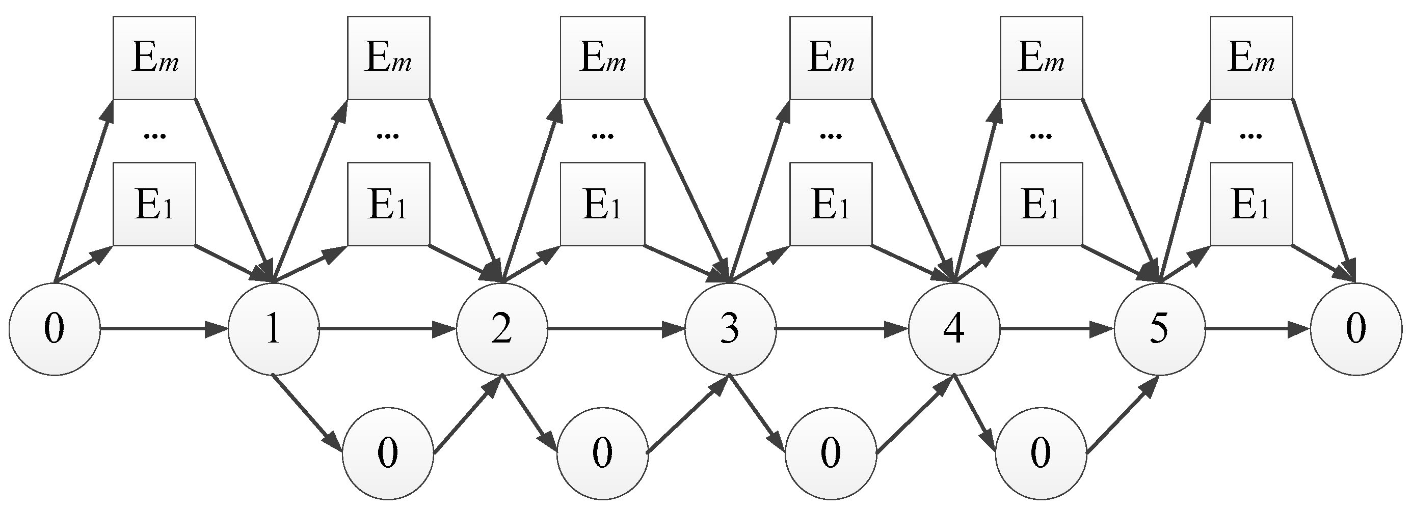
The removal and insertion heuristics and local search do not alter the charging stations of routes in the solution. To obtain the optimal charging stations or intermediate depots for a given sequence of customers, we first construct an auxiliary graph by adding all charging stations and the depot into the customer sequence. Taking a customer sequence {0, 1, 2, 3, 4, 5, 0} as an example, its auxiliary graph is illustrated in Figure 2, where node Ei denotes the charging station and m is the number of charging stations. We need to find a path with minimal cost that starts at Node 0, visits all customers and returns to Node 0. Such a problem can be solved by the labeling algorithm [6,37].
The label algorithm uses labels to construct a partial path from Node 0 to any customer in the sequence. The label at node i is defined as: is the arrival time at node i; and are the total pickup and delivery demand after the last departure from Node 0, respectively; is the maximal demand after the last departure from Node 0; is the total travel distance after the last charge; is the cost from the starting point to node i; is the adjustment cost used and calculated in the dominance rule; and i is the last reached node.
At the starting point 0, are initialized to zero. When a label of customer i is extended to customer j, (m+2) labels are generated, including one label associated with a path directly traveling from customers i to j using the extension rule in Algorithm 2, m labels associated with each path going though one charging station using the extension rule in Algorithm 3, and one label associated with a path going through the depot using the extension rule in Algorithm 4.
| Algorithm 2: Extension rule for directly traveling from customers i to j. | |
| 1: | |
| 2: | if customer j is a delivery node then |
| 3: | , |
| 4: | end if |
| 5: | if customer j is a pickup node then |
| 6: | , |
| 7: | end if |
| 8: | |
| 9: | |
| 10: | ifj is the depot then |
| 11: | |
| 12: | else |
| 13: | |
| 14: | end if |
| Algorithm 3: Extension rule considering charging stations between a pair of nodes. | |
| 1: | |
| 2: | if customer j is a delivery node then |
| 3: | , |
| 4: | end if |
| 5: | if customer j is a pickup node then |
| 6: | , |
| 7: | end if |
| 8: | |
| 9: | , , |
| 10: | ifj is the depot then |
| 11: | |
| 12: | else |
| 13: | |
| 14: | end if |
| Algorithm 4: Extension rule considering depot between a pair of nodes. | |
| 1: | |
| 2: | |
| 3: | |
| 4: | |
| 5: | if customer j is a delivery node then |
| 6: | , |
| 7: | end if |
| 8: | if customer j is a pickup node then |
| 9: | , |
| 10: | end if |
| 11: | |
| 12: | |
An exponential number of labels will be generated during the extension process. Therefore, a dominance rule is essential to remove the labels that cannot lead to optimal paths. The rule is defined as follows.
Definition 1 (Dominance rule):
If two labelsandend at customer i, then label l dominates l′ if,,,,, and at least one of the inequalities is strict.
The arrival time of label l is earlier than that of label l′, which does not guarantee that the cost of the former is smaller than that of the latter during the later extension. Therefore, we adjust the arrival time of label l to the same as that of label l′, compute the adjustment cost , and identify the dominance relationship between the two labels. The adjustment cost is computed as follows.
The notation used in the labeling algorithm is listed as: Li is the set of labels associated with customer i; li is one label associated with customer i; and vi and ns are the ith node and the number of customers in the sequence {v0, v1,…,vi,…,, }, where v0 and denote depot 0. The pseudo code of the labeling algorithm is presented as Algorithm 5.
| Algorithm 5: Labeling algorithm. | |
| 1: | |
| 2: | fori = 1 to ns+1 do |
| 3: | |
| 4: | end for |
| 5: | fori = 1 to ns do |
| 6: | for do |
| 7: | extend to generate using extension rules in Algorithms 2, 3 and 4 |
| 8: | add into using dominance rule in Definition 1 |
| 9: | end do |
| 10: | end do |
| 11: | return the path corresponding to the least-cost label in |
4.9. Departure Time Adjustment Heuristic
The waiting cost in the objective function depends on the first departure time from the depot. We devise a departure time adjustment heuristic to compute the optimal departure time for a given route whose first departure time is zero. The heuristic relies on the difference between the arrival time and time window of each customer. Taking a route {v0, v1,…,vi,…,, } as an example, where vi and ns are the ith node and the number of nodes except the starting and ending nodes. The details of the heuristic are described as Algorithm 6. It first sets the departure time from the depot to zero on Line 1, and then on Lines 2–11 calculates the difference between the arrival time and time window of each customer vi, i.e., and . The adjustment iterative process is described on Lines 12–35. In each iteration, the first customer that incurs a waiting cost and the maximal allowable adjustment time are found on Lines 14–22, and the values of , , and are updated on Lines 23–33. The iterative process continues until the value of at customer vi is zero.
| Algorithm 6: Departure time adjustment heuristic. | |
| 1: | |
| 2: | fori = 0 to ns do // initialize and |
| 3: | , , |
| 4: | if vi+1 is a customer node then |
| 5: | |
| 6: | else if vi+1 is a depot node then |
| 7: | |
| 8: | else if vi+1 is a charging station then |
| 9: | |
| 10: | end if |
| 11: | end for |
| 12: | repeat |
| 13: | , |
| 14: | for i = 0 to ns do |
| 15: | if then // find the first customer which incurs waiting cost |
| 16: | |
| 17: | break |
| 18: | end if |
| 19: | if then // determine the maximal adjustment time |
| 20: | |
| 21: | end if |
| 22: | end for |
| 23: | if then // update the first departure time |
| 24: | if then |
| 25: | |
| 26: | break |
| 27: | else |
| 28: | for i = 1 to do |
| 29: | |
| 30: | end for |
| 31: | , |
| 32: | end if |
| 33: | end if |
| 34: | until |
| 35: | return |
4.10. Set-Partitioning Model
The set Rmodel is populated during the iterations of the ALNS using feasible routes of the local optimum at each iteration. When adding the routes in Rmodel, we check their feasibility and remove the routes with the same set of customers and larger route costs. After the iterative process of the ALNS, we use the set Rmodel to construct a set-partitioning model as follows.
where cr is the route cost of route r; αri is 1 if customer i is visited by route r and otherwise 0; and xr is a 0–1 decision variable that is 1 if route r is selected in the optimal solution and otherwise 0. When the travel time and distance between two customers respect the triangle inequality, the “=“ in the constraints in Equation (4) can be replaced by “≥” (i.e., the set-covering model).
We solve such a model using optimization software and expect that some better solutions missed by the ALNS can be found. To reduce the runtime of solving the model, the best solution obtained by the ALNS is used as an initial solution of the model. Meanwhile, the optimization software continues until the optimal solution of the model is obtained or the maximal runtime exceeds the predefined time TIP.
5. Computational Experiments
In this section, we first introduce the construction of test instances from real-world data provided by a logistics company in Wuhan, China. Then, we report the values of major parameters in the proposed algorithm. Finally, we validate the effectiveness of the proposed algorithm by testing the instances. The algorithm was coded in C++ language. The mathematical model was solved by IBM ILOG CPLEX 12.6.3. All experiments were run on a computer with Intel Xeon E5-1620 V4 3.50 GHz CPU and 32 GB RAM under Windows 10 operating system.
5.1. Construction of Test Instances
The test instances were obtained from real-life data provided by a logistics company in Wuhan, China. The company uses two types of electric vehicles to provide logistics services for customers. The details of electric vehicles are listed in Table 1. The company also has detailed information about customers and charging stations, such as their locations. To generate the instances, we randomly selected approximately 100 customers and 10 charging stations around a distribution center. The loading or unloading time (ti) at each customer is 20 min. If a vehicle returns to the distribution center, it must wait 40 min () to prepare for the next trip. The waiting cost per minute () is 0.5. Twenty instances were generated to validate the effectiveness of the proposed algorithm. Instances are represented in the following format: R1 indicates the first instance in the set.
5.2. Parameter Settings
The parameters of the proposed algorithm are listed in Table 2. To set all parameters, each parameter in turn took several values, while the others were fixed. We ran the proposed algorithm 10 times for each parameter setting, and the parameter setting producing the best average results was selected. Table 2 also shows the best parameter setting for the proposed algorithm.
According to a series of preliminary experiments, the number of customers removed by removal heuristics (q) had the largest influence on the performance of the proposed algorithm. To give a sensitivity analysis to this parameter, six different intervals were tested: [0.05|N|, 0.25|N|], [0.1|N|, 0.3|N|], [0.05|N|, 0.35|N|], [0.1|N|, 0.4|N|], [0.15|N|, 0.35|N|], and [0.15|N|, 0.45|N|]. At each iteration of the ALNS, q was selected uniformly at random in corresponding interval. Table 3 shows the average of the objective function value of all instances in different intervals. The results prove that [0.1|N|, 0.4|N|] was among the best of all intervals.
5.3. Performance Analysis of ALNS
In the proposed algorithm, the best solution obtained by the ALNS is further improved by set-partitioning-based integer programming. To validate the effectiveness of such an algorithm design, we compared the results only using the ALNS with those improved by integer programming (IP). Meanwhile, in the original framework of ALNS, the local search component does not exist. Therefore, we also tested the original ALNS without using the improvement strategies. For each instance, we ran the algorithms ten times. In Table 4, the column “Customers” presents the number of customers included in the instance; the column “Charging Stations” denotes the number of charging stations that can be used in the instance; and the columns “Min”, “Avg”, and “Std” are the minimal, average, and standard deviation, respectively, of objective function values in ten runs. The column “Original ALNS” lists the results of instances obtained by the original ALNS; sub-columns “ALNS” and “IP” in the column “Proposed Algorithm” report the results of instances obtained by the ALNS and improved by the IP, respectively; and the column “Gap” is the relative gap of the minimal objective function value obtained by the corresponding algorithm and proposed algorithm.
From the results listed in Table 4, for all instances, the minimal and average of the objective function values (i.e., total operational cost) obtained by the original ALNS was greater than that found by our proposed algorithm; their average relative gap reached 0.82%. Meanwhile, the average standard deviation of the objective function values obtained by the original ALNS was also larger than that obtained by the proposed algorithm. These results demonstrate the effectiveness of the improved strategies (i.e., the local search component and the IP component) used in the proposed algorithm.
For all instances, in the proposed algorithm, the minimal and average of the total operational cost obtained by the ALNS was not smaller than that improved by the IP; the relative gap between the two algorithm components in the proposed algorithm was between 0% (R7 and R9) and 1.49% (R6), and the average relative gap was 0.40%. These results underline the necessity of the IP components employed in the proposed algorithm.
The runtime for both the original ALNS and the ALNS phase in the proposed algorithm was 600 s. The runtime for solving the set-partitioning model by CPLPEX varied between 0.48 (R9) and 180 s (the maximal runtime set for solving the model, R12), meaning that CPLEX did not solve the model optimally for all test runs. According to our experiments, if CPLEX solved the model to optimality, it might take several hours without improving the solution obtained in the current runtime setting.
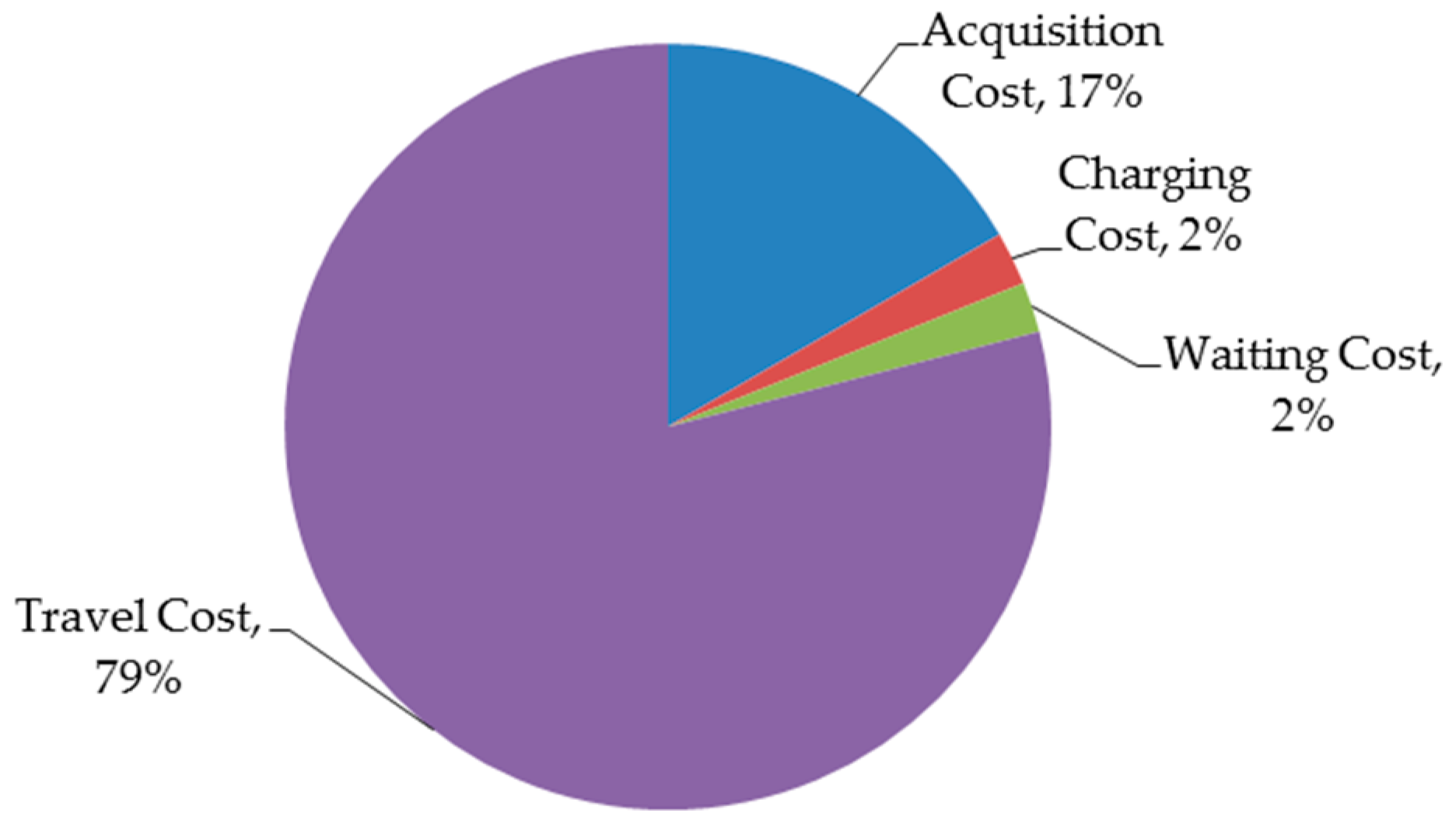
As shown in Table 1, the acquisition cost and travel cost per kilometer of type-2 vehicles are larger than that of type-1 vehicles. If all demands of customers do not exceed the capacity of type-1 vehicles, customers are always visited by type-1 vehicles according to our experiments. Taking the best solution of R1 as an example, it uses 10 type-1 vehicles, charges six times, waits 509 min, and travels 949.707 km. Then, the total acquisition cost is 2000 Yuan, the total charging cost is 270 Yuan, the total waiting cost is 254.5 Yuan, and the total travel cost is 9497.07 Yuan. As shown in Figure 3, the total travel cost is 79% of the total operational cost, indicating that designing reasonable visiting routes is essential for companies to save operational cost.
5.4. Comparison with Company’s Algorithm
The logistics company uses optimization software developed by a consulting company to address the proposed EVRP. To further demonstrate the performance of our algorithm, we compared the results obtained by it with that by optimization software. Due to the confidentiality agreement, the core algorithm embedded in the software cannot be described in detail. The results of instances obtained by the software and the ALNS are listed in Table 5. In the table, the column “Customers” presents the number of customers included in the instance; the column “Charging Stations” denotes the number of charging stations that can be used in the instance; the column “Company’s Algorithm” shows the results of instances obtained by the software; the column “Proposed Algorithm” lists the best results of instances obtained by our algorithm; and the column “Gap” demonstrates the relative gap between the software and our algorithm and equals (Proposed Algorithm − Company’s Algorithm)/Proposed Algorithm × 100%.
Table 5 shows that for all instances the proposed algorithm outperformed the optimization software used in the company. The minimal and maximal relative gaps between the two approaches were 4.49% (R6) and 9.91% (R2), respectively, and the average relative gap was 7.52%, indicating that using our algorithm could save 7.52% of operational cost. We showed the solutions obtained by our algorithm to the managers in the company, and they were very satisfied with these solutions, which can be directly used in practice. These results clearly show the effectiveness of our proposed algorithm.
6. Conclusions and Future Research Works
This paper develops a heuristic approach to solve a real-world EVRP proposed by a logistics company in Wuhan, China. In the approach, the ALNS is followed by solving a set-partitioning mathematical model that strengthens its effectiveness. Meanwhile, to reduce charging costs and waiting costs, two problem-specific heuristics, including the charging station adjustment heuristic and the departure time adjustment heuristic, are devised. The performance of the proposed algorithm was validated by 20 test instances generated from real-world data. The contributions of this paper are summarized as follows. First, this paper investigates a new variant of VRPs that originates from a real-world application and combines the features of different VRPs. Second, an efficient approach based on the ALNS and IP is developed to solve it. In the approach, a charging station adjustment heuristic and a departure time adjustment heuristic are devised to accommodate the features of the proposed problem. Third, the superiority of the proposed approach over the original ALNS is validated through computational experiments.
This work also offers several directions for future research. First, different charge strategies, such as allowing partial charges, will be included in the proposed problem. Second, different charge techniques, such as different charging modes, will be considered in the proposed problem. Finally, different meta-heuristics, such as the genetic algorithm [38] and the VNS [39], will be developed to enrich the solution approaches to the proposed problem.
Author Contributions
Conceptualization, Y.L.; methodology, Y.L. and M.Z.; investigation, M.Z.; writing—original draft preparation, M.Z.; writing—review and editing, Y.L.; supervision, Y.L.; and funding acquisition, Y.L.
Funding
This work was supported by the research grant from the National Natural Science Foundation of China (71801058) and Guangxi Natural Science Foundation (2018JJB110017).
Conflicts of Interest
The authors declare no conflict of interest.
References
- Toth, P.; Vigo, D. Models, Relaxations and Exact Approaches for the Capacitated Vehicle Routing Problem. Discrete. Appl. Math. 2002, 123, 487–512. [Google Scholar] [CrossRef]
- Braysy, I.; Gendreau, M. Vehicle Routing Problem with Time Windows, Part I: Route Construction and Local Search Algorithms. Transp. Sci. 2005, 39, 104–118. [Google Scholar] [CrossRef]
- Braysy, I.; Gendreau, M. Vehicle Routing Problem with Time Windows, Part II: Metaheuristics. Transp. Sci. 2005, 39, 119–139. [Google Scholar] [CrossRef]
- Dell’Amico, M.; Monaci, M.; Pagani, C.; Vigo, D. Heuristic Approaches for the Fleet Size and Mix Vehicle Routing Problem with Time Windows. Transp. Sci. 2007, 41, 516–526. [Google Scholar] [CrossRef]
- Cattaruzza, D.; Absi, N.; Feillet, D. The Multi-Trip Vehicle Routing Problem with Time Windows and Release Dates. Transp. Sci. 2016, 50, 676–693. [Google Scholar] [CrossRef]
- Hiermann, G.; Puchinger, J.; Ropke, S.; Hartl, R.F. The Electric Fleet Size and Mix Vehicle Routing Problem with Time Windows and Recharging Stations. Eur. J. Oper. Res. 2016, 252, 995–1018. [Google Scholar] [CrossRef] [Green Version]
- Arnau, Q.; Juan, A.A.; Serra, I. On the Use of Learnheuristics in Vehicle Routing Optimization Problems with Dynamic Inputs. Algorithms 2018, 11, 208. [Google Scholar] [CrossRef]
- Cassettari, L.; Demartini, M.; Mosca, R.; Revetria, R.; Tonelli, F. A Multi-Stage Algorithm for a Capacitated Vehicle Routing Problem with Time Constraints. Algorithms 2018, 11, 69. [Google Scholar] [CrossRef]
- Chen, S.; Chen, R.; Gao, J. A Monarch Butterfly Optimization for the Dynamic Vehicle Routing Problem. Algorithms 2017, 10, 107. [Google Scholar] [CrossRef]
- Pelletier, S.; Jabali, O.; Laporte, G. Goods Distribution with Electric Vehicles: Review and Research Perspectives. Transp. Sci. 2016, 50, 3–22. [Google Scholar] [CrossRef]
- Schneider, M.; Stenger, A.; Goeke, D. The Electric Vehicle-Routing Problem with Time Windows and Recharging Stations. Transp. Sci. 2014, 48, 500–520. [Google Scholar] [CrossRef]
- Felipe, Á.; Ortuño, M.T.; Righini, G.; Tirado, G. A Heuristic Approach for the Green Vehicle Routing Problem with Multiple Technologies and Partial Recharges. Transport. Res. E-Log. 2014, 71, 111–128. [Google Scholar] [CrossRef]
- Sassi, O.; Cherif-Khettaf, W.R.; Oulamara, A. Iterated Tabu Search for the Mix Fleet Vehicle Routing Problem with Heterogenous Electric Vehicles. Model. Comput. Optim. Inf. Syst. Manag. Sci. 2015, 359, 57–68. [Google Scholar] [CrossRef]
- Yang, J.; Sun, H. Battery Swap Station Location-Routing Problem with Capacitated Electric Vehicles. Comput. Oper. Res. 2015, 55, 217–232. [Google Scholar] [CrossRef]
- Wen, M.; Linde, E.; Ropke, S.; Mirchandani, P.; Larsen, A. An Adaptive Large Neighborhood Search Heuristic for the Electric Vehicle Scheduling Problem. Comput. Oper. Res. 2016, 76, 73–83. [Google Scholar] [CrossRef]
- Keskin, M.; Çatay, B. Partial Recharge Strategies for the Electric Vehicle Routing Problem with Time Windows. Transport. Res. C-Emer. 2016, 65, 111–127. [Google Scholar] [CrossRef]
- Desaulniers, G.; Errico, F.; Irnich, S.; Schneider, M. Exact Algorithms for Electric Vehicle-Routing Problems with Time Windows. Oper. Res. 2016, 64, 1388–1405. [Google Scholar] [CrossRef]
- Montoya, A.; Guéret, C.; Mendoza, J.E.; Villegas, J.G. The Electric Vehicle Routing Problem with Nonlinear Charging Function. Transport. Res. B-Meth. 2017, 103, 87–110. [Google Scholar] [CrossRef]
- Schiffer, M.; Walther, G. The Electric Location Routing Problem with Time Windows and Partial Recharging. Eur. J. Oper. Res. 2017, 260, 995–1013. [Google Scholar] [CrossRef]
- Hof, J.; Schneider, M.; Goeke, D. Solving the Battery Swap Station Location-Routing Problem with Capacitated Electric Vehicles Using an AVNS Algorithm for Vehicle-Routing Problems with Intermediate Stops. Transport. Res. B-Meth. 2017, 97, 102–112. [Google Scholar] [CrossRef]
- Zhang, S.; Gajpal, Y.; Appadoo, S.S.; Abdulkader, M.M.S. Electric Vehicle Routing Problem with Recharging Stations for Minimizing Energy Consumption. Int. J. Prod. Econ. 2018, 203, 404–413. [Google Scholar] [CrossRef]
- Macrina, G.; di Puglia Pugliese, L.; Guerriero, F.; Laporte, G. The Green Mixed Fleet Vehicle Routing Problem with Partial Battery Recharging and Time Windows. Comput. Oper. Res. 2019, 101, 183–199. [Google Scholar] [CrossRef]
- Froger, A.; Mendoza, J.E.; Jabali, O.; Laporte, G. Improved Formulations and Algorithmic Components for the Electric Vehicle Routing Problem with Nonlinear Charging Functions. Comput. Oper. Res. 2019, 104, 256–294. [Google Scholar] [CrossRef]
- Erdoğan, S.; Miller-Hooks, E. A Green Vehicle Routing Problem. Transport. Res. E-Log. 2012, 48, 100–114. [Google Scholar] [CrossRef]
- Ropke, S.; Pisinger, D. An Adaptive Large Neighborhood Search Heuristic for the Pickup and Delivery Problem with Time Windows. Transp. Sci. 2006, 40, 455–472. [Google Scholar] [CrossRef]
- Demir, E.; Bektaş, T.; Laporte, G. An Adaptive Large Neighborhood Search Heuristic for the Pollution-Routing Problem. Eur. J. Oper. Res. 2012, 223, 346–359. [Google Scholar] [CrossRef]
- Luo, Z.; Qin, H.; Zhang, D.; Lim, A. Adaptive Large Neighborhood Search Heuristics for the Vehicle Routing Problem with Stochastic Demands and Weight-Related Cost. Transport. Res. E-Log. 2016, 85, 69–89. [Google Scholar] [CrossRef]
- Ribeiro, G.M.; Laporte, G. An Adaptive Large Neighborhood Search Heuristic for the Cumulative Capacitated Vehicle Routing Problem. Comput. Oper. Res. 2012, 39, 728–735. [Google Scholar] [CrossRef]
- Hemmelmayr, V.C.; Cordeau, J.F.; Crainic, T.G. An Adaptive Large Neighborhood Search Heuristic for Two-Echelon Vehicle Routing Problems Arising in City Logistics. Comput. Oper. Res. 2012, 39, 3215–3228. [Google Scholar] [CrossRef]
- Masson, R.; Lehuede, F.; Peton, O. An Adaptive Large Neighborhood Search for the Pickup and Delivery Problem with Transfers. Transp. Sci. 2013, 47, 344–355. [Google Scholar] [CrossRef]
- Franceschetti, A.; Demir, E.; Honhon, D.; van Woensel, T.; Laporte, G.; Stobbe, M. A Metaheuristic for the Time-Dependent Pollution-Routing Problem. Eur. J. Oper. Res. 2017, 259, 972–991. [Google Scholar] [CrossRef]
- Grangier, P.; Gendreau, M.; Lehuédé, F.; Rousseau, L.M. An Adaptive Large Neighborhood Search for the Two-Echelon Multiple-Trip Vehicle Routing Problem with Satellite Synchronization. Eur. J. Oper. Res. 2016, 254, 80–91. [Google Scholar] [CrossRef]
- Ho, S.C.; Szeto, W.Y. A Hybrid Large Neighborhood Search for the Static Multi-Vehicle Bike-Repositioning Problem. Transport. Res. B-Meth. 2017, 95, 340–363. [Google Scholar] [CrossRef]
- Kovacs, A.A.; Parragh, S.N.; Doerner, K.F.; Hartl, R.F. Adaptive Large Neighborhood Search for Service Technician Routing and Scheduling Problems. J. Sched. 2012, 15, 579–600. [Google Scholar] [CrossRef]
- Ribeiro, G.M.; Desaulniers, G.; Desrosiers, J.; Vidal, T.; Vieira, B.S. Efficient Heuristics for the Workover Rig Routing Problem with a Heterogeneous Fleet and a Finite Horizon. J. Heuristics 2014, 20, 677–708. [Google Scholar] [CrossRef]
- Savelsbergh, M.W.P. Local Search in Routing Problems with Time Windows. Ann. Oper. Res. 1985, 4, 285–305. [Google Scholar] [CrossRef]
- Montoya, A.; Guéret, C.; Mendoza, J.E.; Villegas, J.G. A Multi-Space Sampling Heuristic for the Green Vehicle Routing Problem. Transport. Res. C-Emer. 2016, 70, 113–128. [Google Scholar] [CrossRef]
- Vidal, T.; Crainic, T.G.; Gendreau, M.; Prins, C. A Hybrid Genetic Algorithm with Adaptive Diversity Management for a Large Class of Vehicle Routing Problems with Time-Windows. Comput. Oper. Res. 2013, 40, 475–489. [Google Scholar] [CrossRef]
- Imran, A.; Salhi, S.; Wassan, N.A. A Variable Neighborhood-Based Heuristic for the Heterogeneous Fleet Vehicle Routing Problem. Eur. J. Oper. Res. 2009, 197, 509–518. [Google Scholar] [CrossRef]
Figure 1.
Illustration for the proposed problem.

Figure 2.
Auxiliary graph in the labeling algorithm.

Figure 3.
Percentages of costs of the best solution of R1.


Table 1.
Parameters of electric vehicles.
| Type | Load Capacity Qk (Ton) | Range Dk (Kilometer) | Charging Time (Minute) | Charging Cost per Minute (Yuan) | Acquisition Cost (Yuan) | Travel Cost per Kilometer (Yuan) |
|---|---|---|---|---|---|---|
| 1 | 2.0 | 100 | 30 | 1.5 | 200 | 10 |
| 2 | 2.5 | 150 | 30 | 1.5 | 400 | 12 |
Table 2.
Values for the parameters of the proposed algorithm after the tuning phase.
| Parameter | Meaning | Value |
|---|---|---|
| TALNS | Defines the runtime (seconds) of the ALNS stage | 600 |
| (α0, β0, γ0) | Defines the initial penalty weights of time window, capacity, and battery capacity violations | (100.0, 100.0, 100.0) |
| (αmin, βmin, γmin) | Defines the minimal penalty weights of time window, capacity, and battery capacity violations | (0.001, 0.1, 0.001) |
| (αmax, βmax, γmax) | Defines the maximal penalty weights of time window, capacity, and battery capacity violations | (10,000.0, 1,000,000.0, 1000.0) |
| ω | Adjusts the penalty weights of violations | 1.25 |
| σ1 | Defines the score if a pair of removal and insertion heuristics finds a new global best solution | 33 |
| σ2 | Defines the score if a pair of removal and insertion heuristics finds a new solution that has not been accepted before and is better than the current one | 9 |
| σ3 | Defines the score if a pair of removal and insertion heuristics finds a new non-improving solution that has not been accepted before but is accepted in current iteration | 13 |
| γ | Controls how quickly the weight adjustment reacts to changes in the effectiveness of the heuristics | 0.1 |
| q | Defines the number of customers removed at each iteration | [0.1|N|, 0.4|N|] |
| pShaw | Determines the degree of randomization in Shaw removal | 3 |
| pworst | Determines the degree of randomization in worst removal | 3 |
| phistorical | Determines the degree of randomization in historical knowledge node removal | 5 |
| c | Defines the cooling rate in the simulated annealing | 0.99975 |
| w | Defines the initial temperature control parameter | 0.0005 |
| TIP | Defines the runtime (seconds) of the IP stage | 180 |
Table 3.
Parameter settings for q.
| q | [0.05|N|, 0.25|N|] | [0.1|N|, 0.3|N|] | [0.05|N|, 0.35|N|] | [0.1|N|, 0.4|N|] | [0.15|N|, 0.35|N|], | [0.15|N|, 0.45|N|] |
|---|---|---|---|---|---|---|
| Avg. Obj. | 12,690.22 | 12,632.71 | 12,528.81 | 12,378.87 | 12,430.25 | 12,462.68 |
Table 4.
Results of instances obtained by the proposed algorithm.
| Instance | Customers | Charging Stations | Original ALNS | Proposed Algorithm | ||||||||||
|---|---|---|---|---|---|---|---|---|---|---|---|---|---|---|
| Min | Avg | Std | Gap (%) | ALNS | IP | |||||||||
| Min | Avg | Std | Gap (%) | Min | Avg | Std | CPU (s) | |||||||
| R1 | 110 | 10 | 12,148.00 | 12,197.20 | 29.73 | 1.05 | 12,042.60 | 12,068.10 | 16.03 | 0.17 | 12,021.57 | 12,026.50 | 8.11 | 10.76 |
| R2 | 101 | 10 | 12,721.60 | 12,800.00 | 67.41 | 1.11 | 12,598.90 | 12,652.00 | 33.84 | 0.14 | 12,581.40 | 12,586.40 | 10.02 | 15.92 |
| R3 | 110 | 6 | 8701.49 | 8861.23 | 64.58 | 0.68 | 8661.04 | 8717.05 | 24.27 | 0.22 | 8642.34 | 8650.05 | 9.38 | 2.22 |
| R4 | 108 | 7 | 11,019.90 | 11,062.30 | 35.32 | 0.61 | 11,044.80 | 11,054.50 | 8.50 | 0.84 | 10,952.90 | 11,009.10 | 26.29 | 103.35 |
| R5 | 103 | 8 | 13,875.60 | 13,924.10 | 40.16 | 2.56 | 13,612.40 | 13,674.30 | 37.84 | 0.61 | 13,529.20 | 13,597.30 | 49.17 | 178.07 |
| R6 | 104 | 5 | 13,104.30 | 13,169.20 | 55.72 | 2.02 | 13,037.00 | 13,082.50 | 31.53 | 1.49 | 12,845.00 | 12,915.80 | 41.21 | 167.13 |
| R7 | 100 | 8 | 10,811.90 | 10,852.90 | 27.75 | 0.62 | 10,745.00 | 10,785.40 | 25.71 | 0.00 | 10,745.00 | 10771.00 | 16.16 | 154.25 |
| R8 | 106 | 6 | 12,988.90 | 13,081.80 | 41.85 | 1.87 | 12,781.00 | 12,815.70 | 20.48 | 0.24 | 12,750.30 | 12,787.30 | 29.80 | 180.18 |
| R9 | 108 | 3 | 7915.11 | 8035.10 | 76.09 | 0.04 | 7912.21 | 7912.74 | 0.85 | 0.00 | 7912.21 | 7912.21 | 0.00 | 0.48 |
| R10 | 109 | 14 | 15,605.50 | 15,781.00 | 95.17 | 1.93 | 15,408.40 | 15,499.00 | 83.30 | 0.64 | 15,310.40 | 15,329.60 | 21.02 | 37.68 |
| R11 | 101 | 3 | 9796.08 | 9799.66 | 16.05 | 0.26 | 9781.13 | 9790.26 | 10.20 | 0.11 | 9770.27 | 9770.27 | 0.00 | 20.47 |
| R12 | 108 | 12 | 14,473.60 | 14,527.40 | 62.52 | 0.31 | 14,527.70 | 14,595.60 | 49.64 | 0.69 | 14,428.20 | 14,514.00 | 55.70 | 180.00 |
| R13 | 105 | 12 | 17,829.80 | 17,838.40 | 59.05 | 0.54 | 17,754.20 | 17,839.50 | 46.77 | 0.12 | 17,733.80 | 17,735.10 | 2.35 | 160.58 |
| R14 | 104 | 4 | 11,264.20 | 11,323.50 | 36.30 | 0.60 | 11,227.00 | 11,256.40 | 17.48 | 0.26 | 11,197.50 | 11,232.80 | 24.46 | 158.90 |
| R15 | 106 | 14 | 14,193.30 | 14,284.20 | 52.38 | 0.16 | 14,181.80 | 14,208.80 | 22.12 | 0.08 | 14,170.40 | 14,174.90 | 5.90 | 29.19 |
| R16 | 111 | 5 | 12,090.80 | 12,166.10 | 43.69 | 0.07 | 12,159.40 | 12,187.90 | 16.64 | 0.63 | 12,082.80 | 12,149.30 | 31.25 | 149.33 |
| R17 | 108 | 7 | 10,975.00 | 11,058.50 | 39.45 | 0.20 | 11,045.90 | 11,058.40 | 8.05 | 0.85 | 10,952.90 | 11,010.60 | 27.03 | 107.51 |
| R18 | 101 | 11 | 16,234.00 | 16,296.60 | 49.25 | 0.33 | 16,273.70 | 16,367.00 | 63.17 | 0.57 | 16,180.90 | 16,199.80 | 22.18 | 12.76 |
| R19 | 103 | 10 | 11,245.70 | 11,326.30 | 44.73 | 0.80 | 11,188.90 | 11,212.80 | 10.57 | 0.29 | 11,156.10 | 11,179.80 | 16.45 | 3.97 |
| R20 | 110 | 10 | 12,108.40 | 12,191.80 | 55.30 | 0.72 | 12,034.60 | 12,058.70 | 15.76 | 0.11 | 12,021.60 | 12,025.50 | 6.32 | 8.55 |
| Avg | - | - | 12,455.16 | 12,528.86 | 49.62 | 0.82 | 12,400.88 | 12,441.83 | 27.14 | 0.40 | 12,349.24 | 12,378.87 | 20.14 | 84.07 |
Table 5.
Results of instances obtained by company’s algorithm and the proposed algorithm.
| Instance | Customers | Charging | Company’s Algorithm | Proposed Algorithm | Gap (%) |
|---|---|---|---|---|---|
| R1 | 110 | 10 | 13,035.38 | 12,021.57 | 8.43 |
| R2 | 101 | 10 | 13,828.70 | 12,581.40 | 9.91 |
| R3 | 110 | 6 | 9328.13 | 8642.34 | 7.94 |
| R4 | 108 | 7 | 11,653.22 | 10,952.90 | 6.39 |
| R5 | 103 | 8 | 14,400.21 | 13,529.20 | 6.44 |
| R6 | 104 | 5 | 13,421.89 | 12,845.00 | 4.49 |
| R7 | 100 | 8 | 11,689.32 | 10,745.00 | 8.79 |
| R8 | 106 | 6 | 13,872.90 | 12,750.30 | 8.80 |
| R9 | 108 | 3 | 8654.32 | 7912.21 | 9.38 |
| R10 | 109 | 14 | 16,287.23 | 15,310.40 | 6.38 |
| R11 | 101 | 3 | 10,532.45 | 9770.27 | 7.80 |
| R12 | 108 | 12 | 15,321.65 | 14,428.20 | 6.19 |
| R13 | 105 | 12 | 18,632.21 | 17,733.80 | 5.07 |
| R14 | 104 | 4 | 12,123.22 | 11,197.50 | 8.27 |
| R15 | 106 | 14 | 15,321.22 | 14,170.40 | 8.12 |
| R16 | 111 | 5 | 13,140.23 | 12,082.80 | 8.75 |
| R17 | 108 | 7 | 11,823.12 | 10,952.90 | 7.95 |
| R18 | 101 | 11 | 17,019.22 | 16,180.90 | 5.18 |
| R19 | 103 | 10 | 11,992.23 | 11,156.10 | 7.49 |
| R20 | 110 | 10 | 13,056.98 | 12,021.60 | 8.61 |
| Avg | - | - | 13,256.69 | 12,349.24 | 7.52 |
© 2019 by the authors. Licensee MDPI, Basel, Switzerland. This article is an open access article distributed under the terms and conditions of the Creative Commons Attribution (CC BY) license (http://creativecommons.org/licenses/by/4.0/).
Share and Cite
MDPI and ACS Style
Zhao, M.; Lu, Y. A Heuristic Approach for a Real-World Electric Vehicle Routing Problem. Algorithms 2019, 12, 45. https://0-doi-org.brum.beds.ac.uk/10.3390/a12020045
AMA Style
Zhao M, Lu Y. A Heuristic Approach for a Real-World Electric Vehicle Routing Problem. Algorithms. 2019; 12(2):45. https://0-doi-org.brum.beds.ac.uk/10.3390/a12020045
Chicago/Turabian StyleZhao, Mengting, and Yuwei Lu. 2019. "A Heuristic Approach for a Real-World Electric Vehicle Routing Problem" Algorithms 12, no. 2: 45. https://0-doi-org.brum.beds.ac.uk/10.3390/a12020045
Note that from the first issue of 2016, this journal uses article numbers instead of page numbers. See further details here.