Article

Deep Learning with a Recurrent Network Structure in the Sequence Modeling of Imbalanced Data for ECG-Rhythm Classifier

1
Intelligent System Research Group, Universitas Sriwijaya, Palembang 30137, Indonesia
2
Faculty of Computer Science, Universitas Sriwijaya, Palembang 30137, Indonesia
3
Faculty of Integrated Technologies, Universiti Brunei Darussalam, Jalan Tungku Link, Gadong, BE 1410, Brunei
4
Mechanical Engineering Department, Faculty of Engineering, Diponegoro University, Jl. Prof. Soedharto SH, Tembalang, Semarang 50275, Indonesia
*
Author to whom correspondence should be addressed.
Submission received: 10 May 2019 / Revised: 2 June 2019 / Accepted: 3 June 2019 / Published: 7 June 2019
(This article belongs to the Special Issue Evolutionary Algorithms in Health Technologies)

Abstract

:
The interpretation of Myocardial Infarction (MI) via electrocardiogram (ECG) signal is a challenging task. ECG signals’ morphological view show significant variation in different patients under different physical conditions. Several learning algorithms have been studied to interpret MI. However, the drawback of machine learning is the use of heuristic features with shallow feature learning architectures. To overcome this problem, a deep learning approach is used for learning features automatically, without conventional handcrafted features. This paper presents sequence modeling based on deep learning with recurrent network for ECG-rhythm signal classification. The recurrent network architecture such as a Recurrent Neural Network (RNN) is proposed to automatically interpret MI via ECG signal. The performance of the proposed method is compared to the other recurrent network classifiers such as Long Short-Term Memory (LSTM) and Gated Recurrent Unit (GRU). The objective is to obtain the best sequence model for ECG signal processing. This paper also aims to study a proper data partitioning ratio for the training and testing sets of imbalanced data. The large imbalanced data are obtained from MI and healthy control of PhysioNet: The PTB Diagnostic ECG Database 15-lead ECG signals. According to the comparison result, the LSTM architecture shows better performance than standard RNN and GRU architecture with identical hyper-parameters. The LSTM architecture also shows better classification compared to standard recurrent networks and GRU with sensitivity, specificity, precision, F1-score, BACC, and MCC is 98.49%, 97.97%, 95.67%, 96.32%, 97.56%, and 95.32%, respectively. Apparently, deep learning with the LSTM technique is a potential method for classifying sequential data that implements time steps in the ECG signal.

1. Introduction

Electrocardiogram (ECG) is a key component of the clinical diagnosis and management of inpatients and outpatients that can provide important information about cardiac diseases [1]. Some cardiac diseases can be recognized only through an ECG signal as has been presented in [2,3,4,5,6]. ECG records electrical signals related to heart activity and producing a voltage-chart cardiac rate and being a cardiological test that has been used in the past 100 years [7]. ECG signals have three different waveforms for each cardiac cycle: P wave, QRS complex, and T wave in normal rate [8]. In other cases, ECG form changes in the T waveform, the ST interval length, and ST elevation. Its morphology causes a cardiac abnormality, i.e., Ischemic Heart Disease (IHD) [9]. The IHD is the single largest cause of the main contributors to the disease burden in developing countries [10]. The two leading manifestations of IHD are angina and Acute Myocardial Infarction (MI) [10]. Angina is the characteristic caused by atherosclerosis leading to stenosis of one or more coronary arteries. Then, MI occurs due to a lack of oxygen demand in the cardiac muscle tissue. If cardiac muscle activity increases, oxygen demand also increases [11]. MI is the most dangerous form of IHD with the highest mortality rate [10].
MI is usually diagnosed by changes in the ECG due to the increase of serum enzymes, such as creatine phosphokinase and troponin T or I [10]. ECG is the most reliable tool for interpreting MI [12,13,14], apart from the emergence of expensive and sophisticated alternatives [7]. However, interpreting MI via morphological ECG is a challenging task due to its significant variation in different patients under different physical conditions [15,16]. To prevent the misinterpretation of MI diagnosis, a study uses the nature of ECG signals in a sequence model is automatically necessary. The sequential model consists of sequences of ordering events, with or without concrete notions of time. The algorithm that is usually used for sequential models is a deep learning technique [17]. Some deep learning algorithms that used the sequential model to interpret MI from ECG signals have been presented in References [12,14]. These studies combine Convolutional Neural Network (CNN) and Long Short-Term Memory (LSTM) architecture to interpret MI only in one (Lead I) or several leads (I, II, V1, V2, V3, V4, V5, V6). A sequence modeling is synonymous with recurrent networks that maintain a vector of hidden activations that are propagated through time for most deep learning practitioners [17].
Basic recurrent network architectures are notoriously difficult to train due to the large increase in the norm of the gradient during training, and the opposite behavior when long term components go exponentially fast to norm zero [18]. Some elaborate architectures are commonly used instead, such as the LSTM [19] and GRU [20,21]. Other architectural innovations and training techniques for recurrent networks have been introduced and continue to be actively explored [22,23,24,25]. Unfortunately, none of these studies suggested which recurrent network is a suitable method for classification.
In the present paper, three sequence model classifiers to classify MI and healthy control of 15-lead ECG signals are discussed. The comparison of the recurrent network algorithms is proposed to automatically interpret MI via ECG signal. The recurrent network classifiers include Recurrent Neural Network (RNN), LSTM, and GRU. The objective is to obtain the optimum sequence model in ECG signal recording. To evaluate the performance of recurrent network classifiers in a sequence model, the metric evaluation is proposed. This study also analyzes classifier performance in imbalanced data that the sample size of the data classes is unevenly distributed, among the class of MI and cardiac normal in healthy control patients [26]. In such situations, the classification method tends to be biased towards the majority class. Therefore, this paper uses metric performance balanced accuracy (BACC) and Matthew’s Correlation Coefficient (MCC) to produce better analysis in imbalanced data of MI [26]. In some studies, the use of leads is an important factor for determining the performance results of classifiers [12,13]. The sequence model classifier can be used for 15-lead ECG instead of only use for one or several leads.

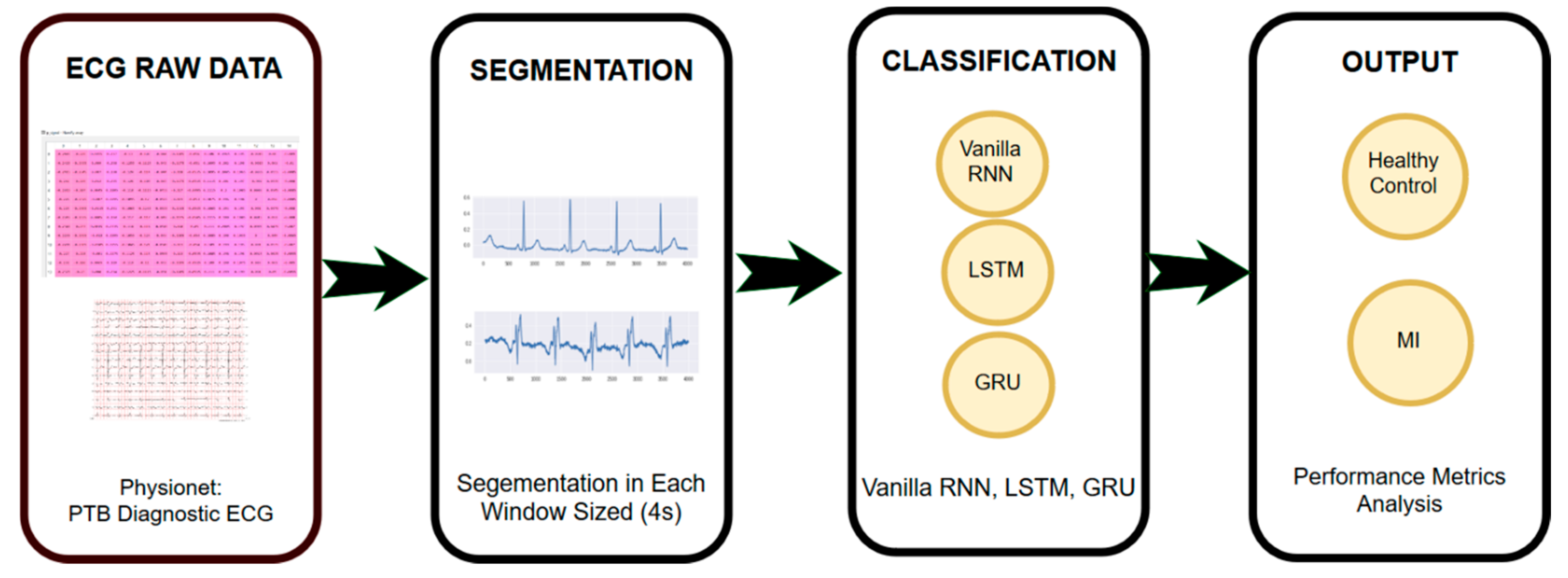
2. Materials and Methods
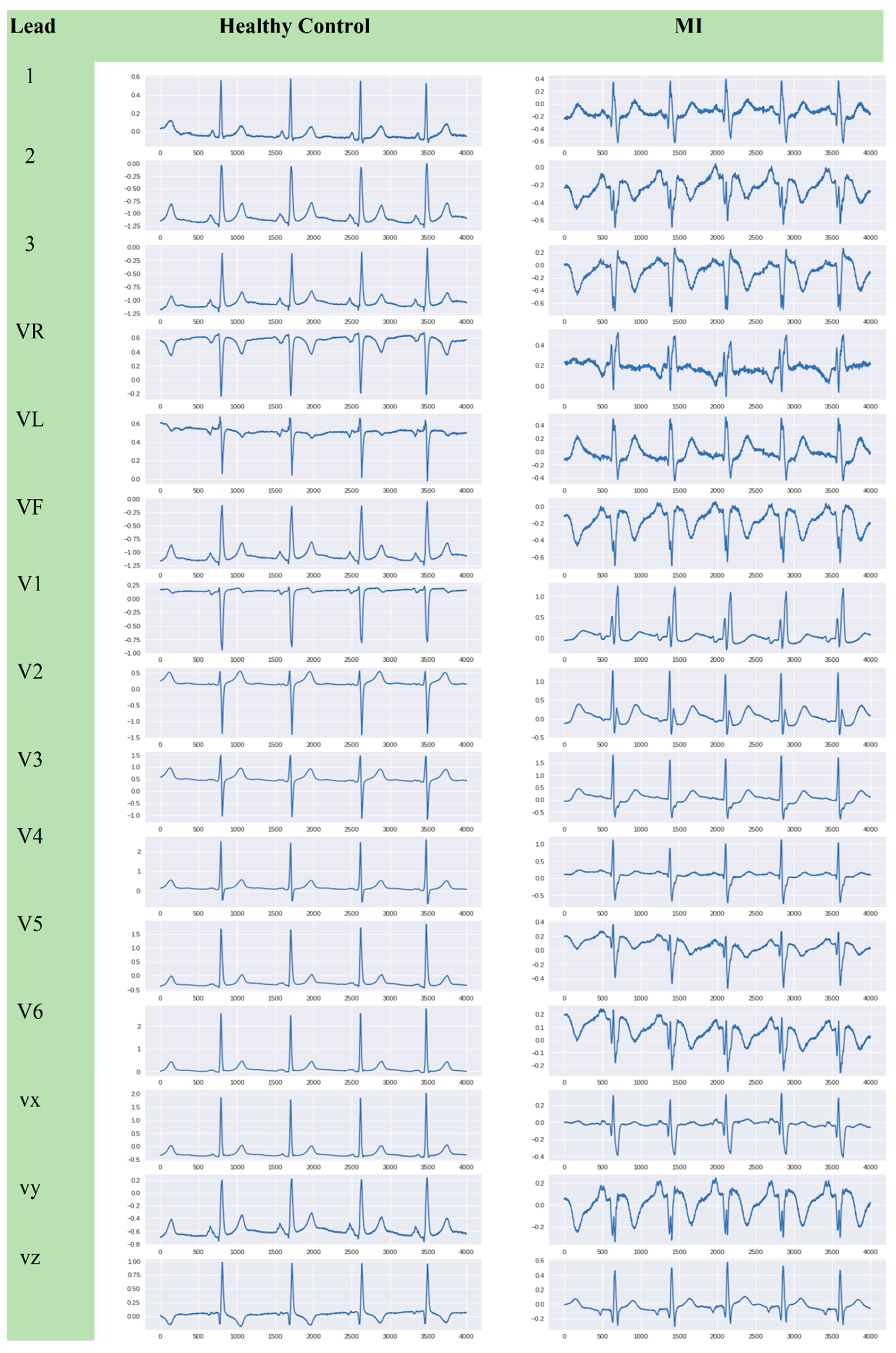
This paper proposes the ECG processing method to calculate appropriate features from 15-lead ECG raw data. The method consists of window sized segmentation, classification of sequence modeling, and evaluation of classifier performance based on performance metrics as presented in Figure 1.

2.1. ECG Raw Data

The sequential data of ECG signals are obtained from the open access database Physionet: PTB Diagnostic ECG, National Metrology Institute of Germany [27]. The PTB Diagnostic ECG database contains 549 records from 290 patients (consisting of 209 males and 81 females). Each patient was associated with one to five ECG record records. Each ECG record includes 15 signals measured simultaneously: 12 conventional leads (I, II, III, aVR, aVL, aVF, V1, V2, V3, V4, V5, and V6) along with 3 Frank leads ECG (vx, vy, vz) in the .xyz file. The PTB Diagnostic ECG database contains ECG signals that represent normal heart conditions and nine heart abnormalities (one of them is MI). However, this study [27] only uses diagnostic classes of healthy controls and myocardial infarction. In fact, there is a number of potential data that can be used for further study which consist of 80 ECG records of the healthy control and 368 ECG records of MI.

2.2. ECG Segmentation

An initial stage of ECG signal pre-processing is the segmentation of the window in the same size. This segmentation is used due to the length of the PTB Diagnostic ECG signal data that varies between each ECG record. The length of the ECG signal for MI ranges from 480000 to 1800180 samples (480–1800 s). For the length of the ECG signal in the healthy control with a range of 1455000–1800180 samples (1455–1800 s). Each window consists of 4 s of data samples at a time, which includes at least three heart beats at a normal heart rate. Each signal has been digitized at 1000 samples per second. A total of 12.359 signal data has been segmented of each window sized for 4 s (see in Figure 2). The number of sequence data for the class of MI and healthy control is 10.144 and 2.215 of the total data, respectively.

2.3. Sequence Modeling Classifier

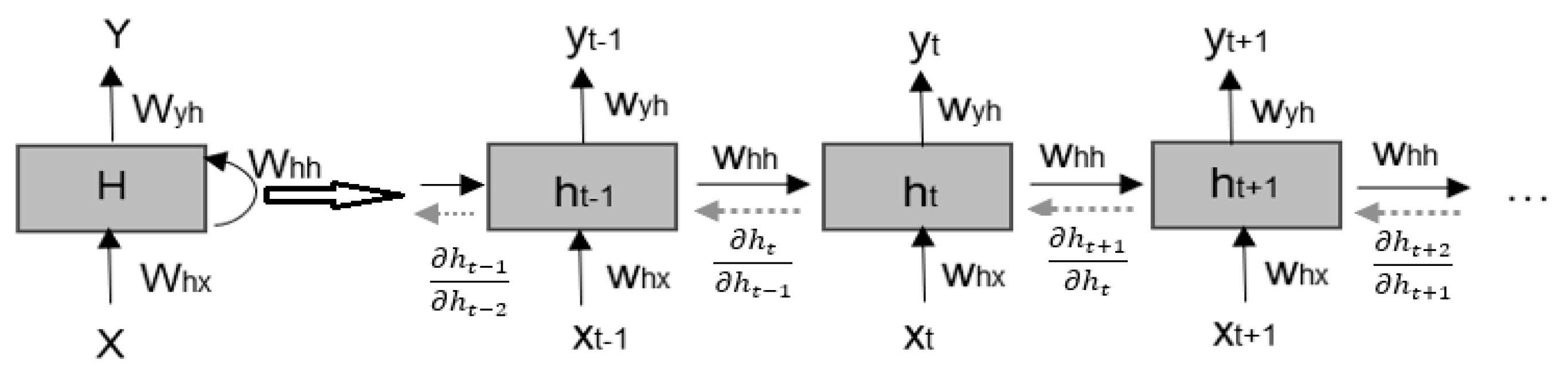
2.3.1. Recurrent Neural Network

Recurrent Neural Network (RNN) is a type of artificial neural network architecture with recurrent connections to process input data [12]. RNN is categorized as a deep learning technique due to an automatic process of feature calculation without predetermining some appropriate features [28]. RNN has “memory”, namely, state ( s t ) that captures information about all input elements ( x t ) to output y ^ t [29]. Original RNN, also known as vanilla RNN, has similar forward pass and backward pass processes as other artificial neural networks. The difference is only in the backpropagation process where the term being backpropagation is defined through time (BPTT) [30].
The model refers to three matrix weights in Figure 3, namely the weight between the input and hidden layers ( w h x R h x ) , the weight between two hidden layers ( w h h R h h ) , and the weights between hidden and output layers ( w y h R y h ) . Otherwise, the bias is added to the hidden layer ( b h R h ) , and the bias vector is added to the output layer ( b y R y ) . The RNN model can be represented in Equations (1) to (3):
h t = f w ( h t 1 , x t )
h t = f ( w h x x t + w h h x t 1 + b h )
y ^ t = f ( w y h h t + b y ) .
It is also well known that the RNN method is sequentially trained method with supervised learning. For step time t, the error results from the difference between the predictions and actual is defined as ( y ^ t y t ) , where, the error or loss is the sum of loss at the time step from t to T :
( y ^ , y ) = t = 1 T ( y ^ t , y t )
Theoretically, the original RNN can handle input dependencies in the long-term, but in practice, the training process of such networks will result to vanishing problems or exploding gradients which is more inefficient when the number of time spans in the input sequence increases [18]. Suppose the ECG data have a total error in all time steps T:
E W = t = 1 T E t W
By applying the chain rules, Equation (5) can be explained as
E W = t = 1 T E y t y t h t h t h k h k W
Equation (6) is a derivative of a hidden state that stores memory at time t which is related to the hidden state at the previous time k. This phase involves the Jacobians matrix for the current time t and one-time k:
h t h k = h t h t 1 h t 1 h t 2 h k + 1 h k = i = k + 1 t h i h i 1
The Jacobian matrix in Equation (7) displays the Eigen Decomposition is given by W T d i a g [ f ( h t 1 ) ] ; the eigenvalues are produced λ 1 , λ 2 , , λ n , where | λ 1 | > | λ 2 | | λ n | and that corresponds to eigenvectors ν 1 , ν 2 , ν n . If the largest eigenvalue is produced λ i < 1 there will be vanishing gradient, on the contrary, if the value of λ i > 1 , then there will be an exploding gradient. To overcome vanishing and exploding gradient problems on RNN standard, LSTM and GRU can be used [18].

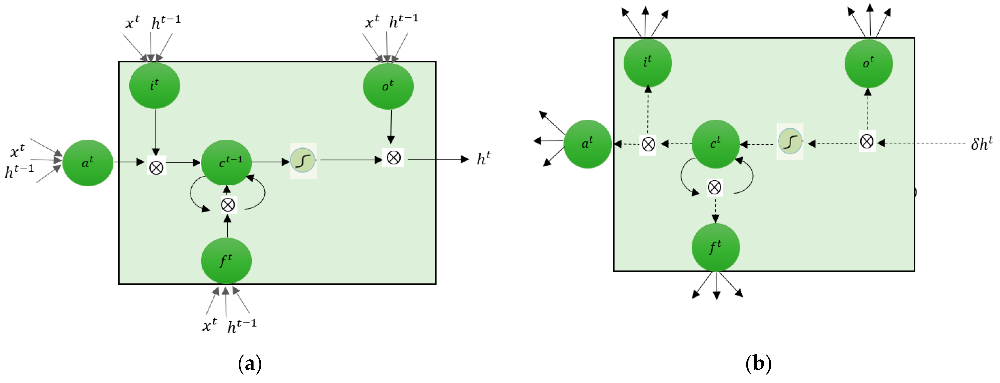
2.3.2. Long Short-Term Memory

The gating mechanism controls the amount of information from the previous time step, which contributes to the current output. Using this gating mechanism, LSTM overcomes vanishing or exploding gradients, wherein a standard RNN there is no gate [29]. The LSTM gate mechanism implements three components; (1) inputs, (2) forget, and (3) output gate [29]. The LSTM input layer must be in 3-dimension vectors (samples, time steps, features). The samples are the amount of train or test set, time steps are 15-lead ECG signals, and features are 4000 samples (4 s) in each window size.
In the LSTM algorithm, the process consists of a forward and backward pass, as shown in Figure 4. A forward pass is calculated as input x with a length T by starting t = 1 and recursively by applying an update equation while adding, t. The scripts i , f and o refer to the input, forget, and output gates from the block, respectively. The script c refers to one of the C memory cells. In time, t, LSTM receives a new input in the form of vector x t (including bias), and the output of the vector h t 1 in the previous time steps (which ⊗ denotes element-wise product Hadamard).
Weights from cell c to input, forget, and output gates are annotated as w i , w f , w o respectively. The equations are given by
a t = tan h ( W c x t + U c h t 1 )
i t = σ ( W i x t + U i h t 1 ) = σ ( i ^ t )
f t = σ ( W f x t + U f h t 1 ) = σ ( f ^ t )
o t = σ ( W o x t + U o h t 1 ) = σ ( o ^ t )
Ignoring the non-linearities,
z t = [ a ^ t i ^ t f ^ t o ^ t ] = [ W c U c W i U i W f U f W o U o ] [ x t h t 1 ] = W I t
Then, the memory cell values updated by combining a t and the contents of the previous cell c t 1 . The combination is based on the magnitude of the gate input i t dan forget gate f t :
c t = i t a t + f t c t 1
In the end, the LSTM cell calculates the output value by passing an updated cell value through non-linearity:
h t = o t f ( c t )
Backward pass computes starting from t = T and recursively calculating the derivative unit in each time step. As standard RNN, all status and activations are initialized to zero at t = 0 , and all δ = 0 at t = T + 1 .

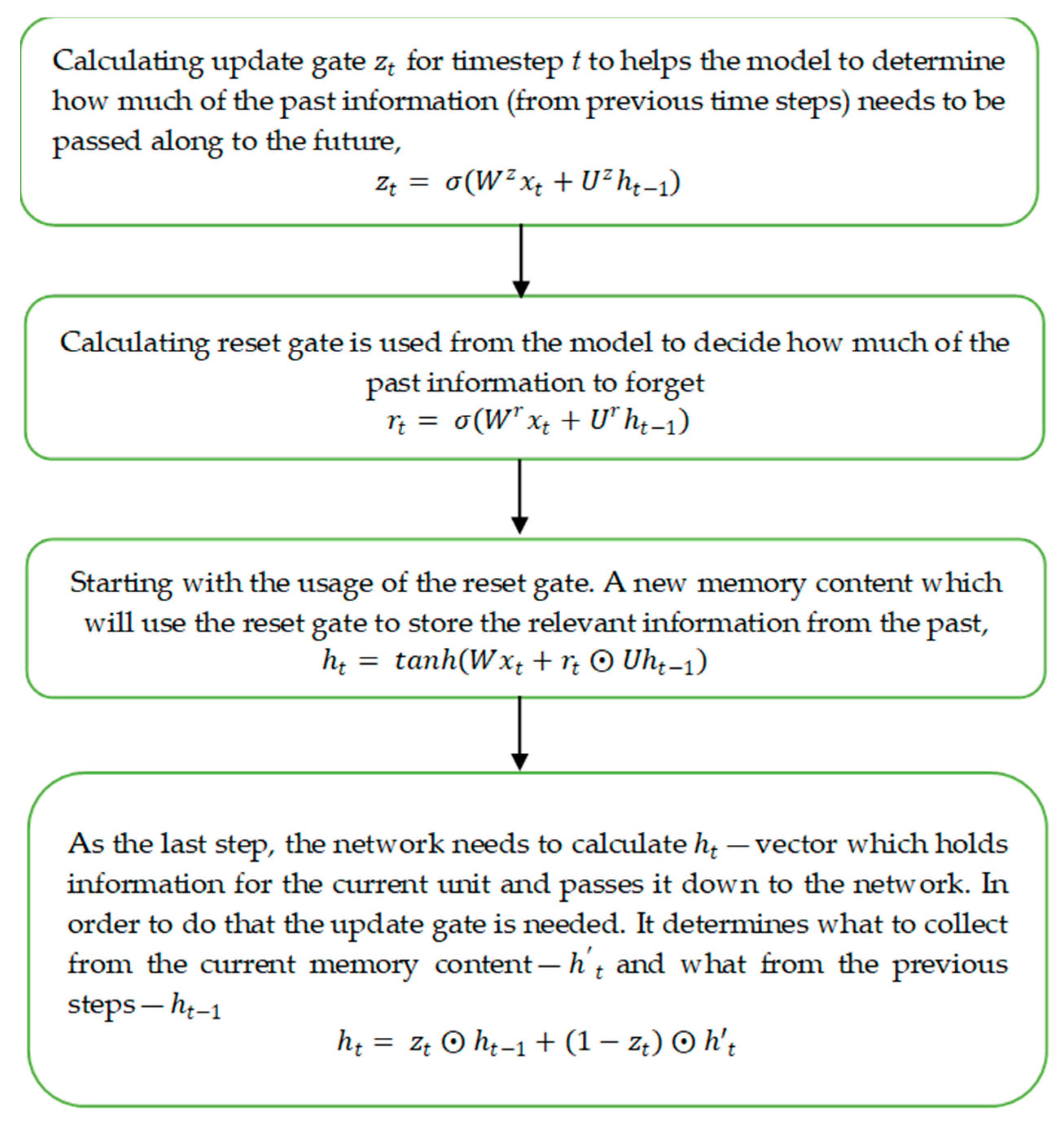
2.3.3. Gated Recurrent Unit

The Gated Recurrent Unit (GRU) architecture consists of two gates: reset gate and update gate [31]. Basically, these are two vectors which decide what information should be passed to the output. Mathematically, the GRU algorithm can be described in the flowchart presented in Figure 5:
The hidden-state model of vanilla RNN, LSTM, and GRU can be represented in the equations listed in Table 1. The difference is in calculating the parameters of each hidden state:

3. Evaluation Performance

The stages of the learning process in neural networks are validated, which is the determination of whether the conceptual model for simulation of the system of interpretation of MI via ECG signals is an accurate representation of the real system being modeled. Evaluation parameters used in the validation process in the binary classification process between the class of MI and normal heart are using confusion matrix, which contains information about the actual classification and predictions made by the classification system. The data in the classification process are divided into two different classes, namely positive (P) and negative (N). This classification produces four types; two types of classifications that are true (or true), namely, true positive (TP) and true negative (TN); and two types of false classifications, namely, false positive (FP) and false negative (FN) [32] (Table 2).
For the overall testing results of the binary classification, in this study, we use the proposed evaluation for binary classification with Balanced Accuracy (BACC) in Equation (15) and Matthew’s Correlation Coefficient (MCC) in Equation (16) for classification in imbalanced data.
B A C C = 1 2 ( T P P + T N N )
M C C = ( T P × T N ) ( F P × F N ) ( T P + F P ) ( T P + F N ) ( T N + F P ) ( T N + F N )

4. Results and Discussion

The comparison of three main sequence models, i.e. Vanilla RNN, LSTM, and GRU is used to classify MI and the healthy control. For all sequence model classifiers, the same hyper-parameters are used. Adam optimization method with learning rate as 0.0001 and 100 epochs were trained in Jupyter Notebook on GPU NVIDIA GeForce RTX 2080. The average of each epoch for the most complex classifier was 13 s. In the sequence model classifier, the number of feed-forward neural network (FFNN) in a unit is different, with vanilla RNN, LSTM, and GRU is one, four, and three FFNN, respectively. The number of FFNN is represented by gates in LSTM and GRU. Knowing the number of FFNN before and after quantization of the sequence model will be useful because it can reduce the size of the model file or even reduce the time needed for model inference.
Furthermore, five different data partitioning ratios of the training and testing set are also compared in the sequence modeling classifier. It consists of 90%:10%, 80%:20%, 70%:30%, 60%:40% and 50%:50% for the training and testing set, respectively (as presented in Table 3). A value of 12.359 of the sequential data is randomly separated with automatic data splitting (shuffled sampling). The training set used is not used for testing and vice versa. We trained all the sequence model classifiers to obtain an optimum model. We have a large imbalanced class of the healthy control and MI i.e., a 4.57 imbalanced ratio. We split the training set to be larger than the testing set initially prior to the data partitioning with the same ratio. As overall, the good result in all data partitioning with training larger than testing set is 90%:10% in all the sequence model classifiers with the average sensitivity, specificity, precision and F1 scores being 90.45%, 94.66%, 93.37% and 91.79%, respectively. Due to having a larger training set, the algorithms are better for understanding the patterns in the set and learning to identify specific examples of training sets. This can optimize the computational time of the validation in the long-term because it can prevent too much overfitting. To evaluate the classifier performance in the imbalanced data, Table 3 describes the results of evaluating binary classifications using BACC and MCC. If the comparison of data between two classes is balanced, it is not recommended to use BACC. The ‘regular’ accuracy metric is sufficient. The average proportion corrects each class individually calculated by BACC. Otherwise, MCC takes values in the interval [−1. 1] with 1 showing a complete agreement and −1 refer to a complete disagreement and 0 showing that the prediction was uncorrelated with label [26]. A coefficient of +1 represents a perfect prediction due to takes into account the balance ratios of the TP, TN, FP and FN categories. The best result in all data partitioning ratio, the average BACC and MCC is 94.81% and 92.98%, respectively.
All data partitioning as presented in Table 3 shows that Vanilla RNN or standard RNN does not learn properly. This problem is due to the vanishing or exploding gradient. The large increase in the norm of the gradient during training and the opposite behavior when long term components go exponentially fast to norm zero. To overcome these problems in standard RNN. LSTM and GRU are used and show better results than Vanilla RNN. The best sequence model classifier is LSTM with 90%:10% for the training and testing set with sensitivity, specificity, precision, F1-score, BACC and MCC is 98.49%, 97.97%, 95.67%, 96.32%, 97.56% and 95.32%, respectively (see in Figure 6 and Figure 7). With our proposed sequence model, specifically the LSTM, MI class can be detected properly.

5. Conclusions

The characteristic of deep learning is to automate feature learning process without hand-crafted creatures. Recurrent network classifiers in a deep learning process that is used for sequential data to binary classification. These classifiers have the characteristic in terms of the number of parameters used in training process. The shared weight in a recurrent network has an advantage due to many fewer parameters to train. The problems of the recurrent network standard have a vanishing or gradient problem. The gating mechanism in LSTM and GRU control some information from the time step to minimize this problem. With fewer ECG pre-processing stages that used in our study, a simple LSTM network presented better classification results of performance in the training and testing setsthan the RNN standard and GRU. It is due to the LSTM method is able to stores more information about the pattern of data compared to the RNN standard and GRU. LSTM is able to learns and selects which data need to be stored or discarded that affects LSTM performance better (forget gates) than other comparable methods. The LSTM structure with 90%:10% for training and testing set presents the sensitivity, specificity, precision and F1-score of 98.49%, 97.97%, 95.67%, and 96.32%, respectively.
Furthermore, to evaluate binary classification in imbalanced data MCC and BACC have a closed form and it is very well suited to be used for building the optimal classifier. However, the performance results in the initial stage show unsatisfied due to the lack of ECG signal processing before being classified by sequence modeling classifier. Our LSTM model suggests the presence of crucial information in 15-lead ECG to predict the future clinical course, especially for detecting chest discomfort in real time.

Author Contributions

A.D. Formal analysis, software, and writing—original draft; S.N. Conceptualization, resources, supervision, and writing—review & editing; S. Writing—original draft and writing—review & editing; W.C. Funding acquisition and writing—review & editing; V.B. Software; M.N.R. Software; F. Writing—original draft and writing—review & editing.

Funding

This research is supported by the Kemenristek Dikti Indonesia under the Basic Research Fund Number. 096/SP2H/LT/DRPM/2019 and Universitas Sriwijaya. Indonesia under Hibah Unggulan Profesi Fund 2019.

Acknowledgments

The authors are very thankful to Reviewers and Wahyu Caesarendra for his valuable comments, discussion and suggestions for improving the paper.

Conflicts of Interest

The authors declare no conflict of interest.

References

  1. Goldberger, A.L.; Goldberger, Z.D.; Shvilkin, A. Clinical Electrocardiography: A Simplified Approach E-Book; Elsevier: Amsterdam, The Netherlands, 2017. [Google Scholar]
  2. Nurmaini, S.; Gani, A. Cardiac Arrhythmias Classification Using Deep Neural Networks and Principal Component Analysis Algorithm. Int. J. Adv. Soft Comput. Appl. 2018, 10, 14–32. [Google Scholar]
  3. Caesarendra, W.; Ismail, R.; Kurniawan, D.; Karwiky, G.; Ahmad, C. Suddent cardiac death predictor based on spatial QRS-T angle feature and support vector machine case study for cardiac disease detection in Indonesia. In Proceedings of the 2016 IEEE EMBS Conference on Biomedical Engineering and Sciences (IECBES), Kuala Lumpur, Malaysia, 4–8 December 2016; pp. 186–192. [Google Scholar]
  4. Pławiak, P. Novel genetic ensembles of classifiers applied to myocardium dysfunction recognition based on ECG signals. Swarm Evol. Comput. 2018, 39, 192–208. [Google Scholar] [CrossRef]
  5. Acharya, U.R.; Fujita, H.; Oh, S.L.; Hagiwara, Y.; Tan, J.H.; Adam, M.; Tan, R.S. Deep convolutional neural network for the automated diagnosis of congestive heart failure using ECG signals. Appl. Intell. 2018, 1–12. [Google Scholar] [CrossRef]
  6. Steinhubl, S.R.; Waalen, J.; Edwards, A.M.; Ariniello, L.M.; Mehta, R.R.; Ebner, G.S.; Carter, C.; Baca-Motes, K.; Felicione, E.; Sarich, T.; et al. Effect of a home-based wearable continuous ECG monitoring patch on detection of undiagnosed atrial fibrillation: The mSToPS randomized clinical trial. JAMA 2018, 320, 146–155. [Google Scholar] [CrossRef] [PubMed]
  7. Khan, M.G. Rapid ECG Interpretation; Springer: Berlin/Heidelberg, Germany, 2008. [Google Scholar]
  8. Fleming, J.S. Interpreting the Electrocardiogram; Springer: Berlin/Heidelberg, Germany, 2012. [Google Scholar]
  9. Zimetbaum, P.J.; Josephson, M.E. Use of the electrocardiogram in acute myocardial infarction. N. Engl. J. Med. 2003, 348, 933–940. [Google Scholar] [CrossRef]
  10. Gaziano, T.; Reddy, K.S.; Paccaud, F.; Horton, S.; Chaturvedi, V. Cardiovascular disease. In Disease Control Priorities in Developing Countries, 2nd ed.; The International Bank for Reconstruction and Development/The World Bank: Washington, DC, USA, 2006. [Google Scholar]
  11. Thygesen, K.; Alpert, J.S.; White, H.D. Universal definition of myocardial infarction. J. Am. Coll. Cardiol. 2007, 50, 2173–2195. [Google Scholar] [CrossRef]
  12. Lui, H.W.; Chow, K.L. Multiclass classification of myocardial infarction with convolutional and recurrent neural networks for portable ECG devices. Inform. Med. Unlocked 2018, 13, 26–33. [Google Scholar] [CrossRef]
  13. Strodthoff, N.; Strodthoff, C. Detecting and interpreting myocardial infarctions using fully convolutional neural networks. arXiv 2018, arXiv:1806.07385. [Google Scholar] [CrossRef]
  14. Goto, S.; Kimura, M.; Katsumata, Y.; Goto, S.; Kamatani, T.; Ichihara, G.; Ko, S.; Sasaki, J.; Fukuda, K.; Sano, M. Artificial intelligence to predict needs for urgent revascularization from 12-leads electrocardiography in emergency patients. PLoS ONE 2019, 14, e0210103. [Google Scholar] [CrossRef]
  15. Mawri, S.; Michaels, A.; Gibbs, J.; Shah, S.; Rao, S.; Kugelmass, A.; Lingam, N.; Arida, M.; Jacobsen, G.; Rowlandson, I.; et al. The comparison of physician to computer interpreted electrocardiograms on ST-elevation myocardial infarction door-to-balloon times. Crit. Pathw. Cardiol. 2016, 15, 22–25. [Google Scholar] [CrossRef]
  16. Banerjee, S.; Mitra, M. Application of cross wavelet transform for ECG pattern analysis and classification. IEEE Trans. Instrum. Meas. 2014, 63, 326–333. [Google Scholar] [CrossRef]
  17. Bai, S.; Kolter, J.Z.; Koltun, V. An empirical evaluation of generic convolutional and recurrent networks for sequence modeling. arXiv 2018, arXiv:1803.01271. [Google Scholar]
  18. Pascanu, R.; Mikolov, T.; Bengio, Y. On the difficulty of training recurrent neural networks. In Proceedings of the International Conference on Machine Learning, Atlanta, GA, USA, 16–21 June 2013; pp. 1310–1318. [Google Scholar]
  19. Hochreiter, S.; Schmidhuber, J. Long short-term memory. Neural Comput. 1997, 9, 1735–1780. [Google Scholar] [CrossRef] [PubMed]
  20. Cho, K.; Van Merriënboer, B.; Gulcehre, C.; Bahdanau, D.; Bougares, F.; Schwenk, H.; Bengio, Y. Learning phrase representations using RNN encoder-decoder for statistical machine translation. arXiv 2014, arXiv:1406.1078. [Google Scholar]
  21. Jia, H.; Deng, Y.; Li, P.; Qiu, X.; Tao, Y. Research and Realization of ECG Classification based on Gated Recurrent Unit. In Proceedings of the 2018 Chinese Automation Congress (CAC), Xi’an, China, 30 November–2 December 2018; pp. 2189–2193. [Google Scholar]
  22. Koutnik, J.; Greff, K.; Gomez, F.; Schmidhuber, J. A clockwork rnn. arXiv 2014, arXiv:1402.3511. [Google Scholar]
  23. Le, Q.V.; Jaitly, N.; Hinton, G.E. A simple way to initialize recurrent networks of rectified linear units. arXiv 2015, arXiv:1504.00941. [Google Scholar]
  24. Krueger, D.; Maharaj, T.; Kramár, J.; Pezeshki, M.; Ballas, N.; Ke, N.R.; Goyal, A.; Bengio, Y.; Courville, A.; Pal, C. Zoneout: Regularizing rnns by randomly preserving hidden activations. arXiv 2016, arXiv:1606.01305. [Google Scholar]
  25. Campos, V.; Jou, B.; Giró-i-Nieto, X.; Torres, J.; Chang, S.-F. Skip rnn: Learning to skip state updates in recurrent neural networks. arXiv 2017, arXiv:1708.06834. [Google Scholar]
  26. Boughorbel, S.; Jarray, F.; El-Anbari, M. Optimal classifier for imbalanced data using Matthews Correlation Coefficient metric. PLoS ONE 2017, 12, e0177678. [Google Scholar] [CrossRef] [PubMed]
  27. Goldberger, A.L.; Amaral, L.A.; Glass, L.; Hausdorff, J.M.; Ivanov, P.C.; Mark, R.G.; Mietus, J.E.; Moody, G.B.; Peng, C.K.; Stanley, H.E. PhysioBank, PhysioToolkit, and PhysioNet: Components of a new research resource for complex physiologic signals. Circulation 2000, 101, e215–e220. [Google Scholar] [CrossRef]
  28. Wiatowski, T.; Bölcskei, H. A mathematical theory of deep convolutional neural networks for feature extraction. IEEE Trans. Inf. Theory 2018, 64, 1845–1866. [Google Scholar] [CrossRef]
  29. Faust, O.; Shenfield, A.; Kareem, M.; San, T.R.; Fujita, H.; Acharya, U.R. Automated detection of atrial fibrillation using long short-term memory network with RR interval signals. Comput. Biol. Med. 2018, 102, 327–335. [Google Scholar] [CrossRef] [PubMed] [Green Version]
  30. Bullinaria, J.A. Recurrent Neural Networks. 2015. Available online: http://www.cs.bham.ac.uk/~jxb/INC/l12.pdf (accessed on 18 February 2019).
  31. Singh, S.; Pandey, S.K.; Pawar, U.; Janghel, R.R. Classification of ECG Arrhythmia using Recurrent Neural Networks. Procedia Comput. Sci. 2018, 132, 1290–1297. [Google Scholar] [CrossRef]
  32. Darmawahyuni, A. Coronary Heart Disease Interpretation Based on Deep Neural Network. Comput. Eng. Appl. J. 2019, 8, 1–12. [Google Scholar] [CrossRef]
Figure 1. Electrocardiogram (ECG) processing.
Algorithms 12 00118 g001
Figure 2. The ECG window sized segmentation in each 4 s.
Algorithms 12 00118 g002
Figure 3. The forward and backward pass in recurrent neural network (RNN) standard [18].
Algorithms 12 00118 g003
Figure 4. (a) Forward, and (b) backward passes in the Long Term-Short Term Memory (LSTM).
Algorithms 12 00118 g004
Figure 5. The Gated Recurrent Unit (GRU) algorithm.
Algorithms 12 00118 g005
Figure 6. The plot of accuracy of the LSTM architecture with 90% of training and 10% of testing set.
Algorithms 12 00118 g006
Figure 7. The plot of loss of the LSTM architecture with 90% of training and 10% of the testing set.
Algorithms 12 00118 g007
Table 1. The Hidden State in Sequence Modeling Classifier.
ClassifierHidden State Model
RNN h t = tan h ( k = 1 t W c t k W i n x k )
LSTM h t = σ ( W o I t ) tan h ( k = 1 t [ j = k + 1 t σ ( W f I j ) ] σ ( W i I k ) tan h ( W i n I k ) )
GRU h t = k = 1 t [ j = k + 1 t σ ( W z I j ) ] ( 1 σ ( W z x k ) ) tan h ( W x k )
Table 2. The Diagnostic Test.
DiagnosticMIHealthy ControlTotal
MITrue Positive (TP)False Positive (FP)All Positive Test (T+)
Healthy ControlFalse Negative (FN)True Negative (TN)All Negative Test (T−)
TotalTotal of MITotal of Healthy ControlTotal Sample
Table 3. The result of the sequence model classifier performance.
Training: Testing (%)Sequence Model ClassifierPerformance Metrics (%)
SensitivitySpecificityPrecisionF1-scoreBACCMCC
90:10Vanilla RNN85.8187.9289.5684.9788.1489.85
LSTM98.4997.9795.6796.3297.5695.32
GRU87.0798.1094.8994.0898.7393.78
80:20Vanilla RNN86.8687.2888.3782.4081.6689.64
LSTM92.4797.6290.1188.5789.8179.62
GRU87.1788.4990.6086.6988.9087.90
70:30Vanilla RNN81.8890.7860.4663.6075.0067.08
LSTM88.1893.6171.5182.5583.3378.78
GRU92.5993.6071.5182.2783.3378.78
60:40Vanilla RNN67.0991.1260.4669.5675.0067.08
LSTM97.6192.1665.1174.9175.0067.08
GRU96.8593.7972.6781.4383.3378.78
50:50Vanilla RNN31.4488.7064.5342.2873.1454.71
LSTM88.1493.0069.1877.5283.3378.78
GRU51.0287.8043.4146.9167.0648.50

