Solution Merging in Matheuristics for Resource Constrained Job Scheduling


1
School of Information Technology, Deakin University, Geelong 3126, Australia
2
Artificial Intelligence Research Institute (IIIA-CSIC), Campus of the UAB, 08193 Bellaterra, Spain
3
School of Mathematics, Monash University, Melbourne 3800, Australia
*
Author to whom correspondence should be addressed.
Algorithms 2020, 13(10), 256; https://0-doi-org.brum.beds.ac.uk/10.3390/a13100256
Submission received: 7 September 2020
/
Revised: 29 September 2020
/
Accepted: 1 October 2020
/
Published: 9 October 2020
(This article belongs to the Special Issue Algorithms for Graphs and Networks)
Abstract
:Matheuristics have been gaining in popularity for solving combinatorial optimisation problems in recent years. This new class of hybrid method combines elements of both mathematical programming for intensification and metaheuristic searches for diversification. A recent approach in this direction has been to build a neighbourhood for integer programs by merging information from several heuristic solutions, namely construct, solve, merge and adapt (CMSA). In this study, we investigate this method alongside a closely related novel approach—merge search (MS). Both methods rely on a population of solutions, and for the purposes of this study, we examine two options: (a) a constructive heuristic and (b) ant colony optimisation (ACO); that is, a method based on learning. These methods are also implemented in a parallel framework using multi-core shared memory, which leads to improving the overall efficiency. Using a resource constrained job scheduling problem as a test case, different aspects of the algorithms are investigated. We find that both methods, using ACO, are competitive with current state-of-the-art methods, outperforming them for a range of problems. Regarding MS and CMSA, the former seems more effective on medium-sized problems, whereas the latter performs better on large problems.
1. Introduction
Large optimisation problems often cannot be solved by off-the-shelf solvers. Solvers based on exact methods (e.g., integer programming and constraint programming) have become increasingly efficient, though, they are still limited in their performance due to large problem sizes and their complexities. Since solving such problems requires algorithms that can still identify good solutions in a time-efficient manner, alternative incomplete techniques, such as integer programming decompositions, as well as metaheuristics and their hybridisations, have been given a lot of attention.
Metaheuristics aim to alleviate the problems associated with exact methods, and have been shown to be very effective across a rage of practical problems [1]. A number of the most effective methods are inspired from nature—for example, evolutionary algorithms [2,3] and swarm intelligence [4,5]. Despite their success, metaheuristics are limited in their applicability as they are especially inefficient when dealing with non-trivial hard constraints. Constraint programming [6] is capable of dealing with complex constraints but does generally not scale well on problems with large search spaces. Mixed integer (linear) programming (MIP) [7] can deal with large search spaces and also deal with complex constraints. However, the efficiency of general purpose MIP solvers drops sharply when reaching a certain, problem-dependent, instance size.
Techniques for solving large problems with MIPs have been an active area of research in the recent past. Decomposition methods such as Lagrangian relaxation [8], column generation [7] and Benders’ decomposition [9] have proved to be effective on a range of problems. Hierarchical models [10] and large neighbourhood search methods have also proven to be successful [11].
Recently, matheuristics, or hybrids of integer programming and metaheuristics, have been gaining in popularity [12,13,14,15,16]. References [12,17] provide an overview of these methods and [13] provide a survey of matheuristics applied to routing problems. The study by [14] shows that nurse rostering problems can be solved efficiently by a matheuristic based on a large neighbourhood search. Reference [15] apply an integer programming based heuristic to a liner shipping design problem with promising results. Reference [16] show that an integer programming heuristic based on Benders’ decomposition is very effective for scheduling medical residents’ training at university hospitals.
This paper focuses on two rather recent novel MIP-based matheuristic approaches, which rely on the concept of solution merging to learn from a population of solutions. Both of these methods use the same basic idea: using a MIP to generate a “merged” solution in the subspace that is spanned by a pool of heuristic solutions. The first is a very recent approach—Merge Search (MS) [18] and the second method is Construct, Merge, Solve and Adapt (CMSA) [19,20,21,22]. The study by [18] shows that MS is well suited for solving the constrained pit problem. Reference [19] apply CMSA to minimum common string partition and to the minimum covering arborescence problem, ref. [20] investigate the repetition-free longest common subsequence problem, and [21] examines the unbalanced common string partition problem. The study by [22] investigates a hybrid of CMSA and parallel ant colony optimisation (ACO) for resource constrained project scheduling. Both MS and CMSA aim to search for high quality solutions to a problem in a similar way: (a) initialise a population of solutions, (b) solve a restricted MIP to obtain a “merged” solution, (c) update the solution population by incorporating new information and (d) repeat until some termination criteria are fulfilled. However, they differ in the details in how they implement these steps.
In principle, a merge step could be added to any heuristic optimisation algorithm that randomly samples the solution space. The question is whether this helps to improve the performance of a heuristic search. Additionally, what type of merge step should be used, given that CMSA and MS use two slightly different merge methods? This study attempts to provide some answers to these questions in the context of a specific optimisation problem.
This study investigates MS and CMSA with the primary aim of comparing the effects of the differences between these related algorithms to better understand what elements are important in obtaining the best performance. The case study used for the empirical evaluation of the algorithms is the Resource Constrained Job Scheduling (RCJS) problem [23]. The RCJS problem was originally motivated by an application from the mining industry and aims to capture the key aspects of moving iron ore from mines to ports. The objective is to minimise the tardiness of batches of ore arriving at ports, which has been a popular objective with other scheduling problems [24,25]. Several algorithms have been attempted on this problem, particularly hybrids incorporating Lagrangian relaxation, column generation, metaheuristics (simulated annealing, ant colony optimisation and particle swarm optimisation), genetic programming, constraint programming and parallel implementations of these methods [23,26,27,28,29,30,31,32]. The problem is a relatively simple-to-state scheduling problem with a single shared resource. Nevertheless, the problem is sufficiently well studied to provide a baseline for performance while still having room for improvement with many larger instances not solved optimally. The primary aim, though, is not to improve the state-of-the-art for this particular type of problem—even though our approaches outperform the state-of-the-art across a number of problem instances—but to get a better understanding of the behaviour of the two considered algorithms.
The paper is organised as follows. First, we briefly summarise the scheduling problem used as a case study and provide some alternative ways of formulating this as a mixed integer linear program (Section 2). Then, in Section 3 we provide the details of the two matheuristic methods MS and CMSA, and we outline how they are applied to the RCJS problem, and discuss briefly the intuition behind these methods. We also discuss ways to generate the population, including a constructive heuristic, ACO and their associated parallel implementations. We detail the motivations for this study in Section 4 and this is followed by an experimental set-up and empirical evaluation in Section 5. Then, a short discussion of the results is given in Section 6. Finally, the paper concludes in Section 7, where possibilities for future work are discussed.
2. Resource Constrained Job Scheduling
The resource constrained job scheduling (RCJS) problem consists of a number of nearly independent single machine weighted tardiness problems that are only linked by a single shared resource constraint. It is formally defined as follows. A number of jobs must execute on machines . Each jobs has the following data associated with it: a release time , a processing time , a due time , the amount required from the resource, a weight , and the machine to which it belongs. The maximum amount of resource available at any time is . Precedence constraints may apply to two jobs on the same machine: requires that job i completes executing before job j starts. Given a sequence of jobs, , the objective is to minimise the total weighted tardiness:
where denotes the completion time of the job at position i of , which—given —can be derived in a well-defined way.
2.1. Network Design Formulation
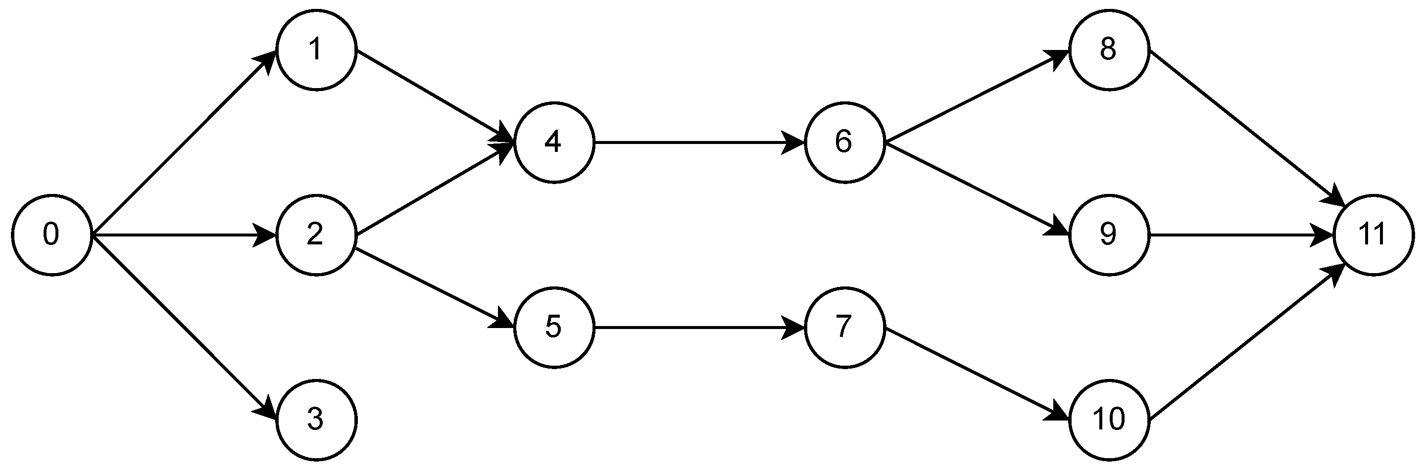
This problem can be thought of as a network design problem to create a directed, acyclic graph representing a partial ordering of the job start times (see Figure 1). Here, node 0 represents the start of the schedule. For any pair of jobs that have a precedence there is an arc with duration separating the start time of the two jobs. Additionally, for any job i that has a release time which is not already implied by the precedence relationships, the graph contains arcs of duration . To capture the tardiness we also introduce an additional dummy node for each .
The problem can now be formulated as follows using variables to denote the start time of node (job) i with , the completion time or due date for job i (this associated with the dummy node ). Finally the binary variables are one if arc is to be added to the graph. Using these variables we can write the network design problem:
Here is the set of all minimal cliques K in the complement of the precedence graph (that is collection of jobs that do not have a given precedence relationship) such that each of the jobs belongs to a different machine and . It should be noted that constraints (3)–(5), which capture the release times, processing time and due date requirement, all have the same form of difference between two variables greater than a constant. The same also applies for (6) for fixed values of the y variables. Hence, for given y variables, this is simply the dual of a network flow problem. This means that, for integer data, the optimal times and will all be integers. Note that the objective (2) includes a constant term () and has the variable with a constant, such that adding a constant to all of the s and u variables does not change the objective. (Without this the problem would be unbounded). Alternatively we could arbitrarily fix . Constraints (7) fix in the given precedence arcs of the network. The remaining constraints on y variables relate to the network design part of the problem. Constraints (8) and (9) enforce a total ordering of jobs on the same machine and a partial ordering amongst the remaining jobs, respectively. Finally, (10) prevents more jobs from running simultaneously (without an ordering) than can be accommodated within the resource limit.
This formulation, while illustrating the network design nature of the problem, suffers from somewhat poor computational performance. While (10) includes a lot of constraints, these can be added as lazy constraints. However the main problem is due to the “big-M” constraints (6), which are very weak. To make this problem more computationally tractable, we will look at time discretization-based formulations next.
2.2. Time Discretised Mixed Integer Programs
There are many ways of formulating this problem as a mixed integer linear program (MIP). Different formulations can be expected to cause MIP solvers to exhibit different performances. More importantly, the MIP formulation acts as a representation or encoding of our solutions and, hence, impacts in more subtle ways on how the heuristics explore the solution space. Therefore, we present two further alternative formulations of the problem. In this section, we restrict ourselves to some basic observations regarding the characteristics of the formulations and defer the discussion of how these interact with the meta-heuristic search until we have presented our search methods. Both of the following formulations rely on data comprising integers so that only discrete times need to be considered.
2.3. Model 1
A common technique in the context of exact methods for scheduling is to discretise time [33]. Let be a set of time intervals (with being sufficiently large) and let be a binary variable for all and , which takes value 1 if the processing of job j completes at time t. By defining the weighted tardiness for a job j at time t as , we can formulate an MIP for the RCJS problem, as follows.
Constraints (12) ensure that all jobs are complete. Constraints (13) ensure that the release times are satisfied and are typically implemented by excluding all of these variables from the model. Constraints (14) take care that the precedences between jobs a and b are satisfied and Constraints (16) ensure that no more than one job is processed at the same time on one machine. Constraints (16) ensure that the resource constraints are satisfied.
This model is certainly the most natural way to formulate the RCJS problem, though not necessarily the computationally most effective. The linear programming (LP) bounds could be strengthened by replacing each precedence constraint of the form (14), with a set of constraints specifying that . Additionally, the branching behaviour for this formulation tends to be very unbalanced: forcing a fractional variable to take value 1 in the branch and the bound tree can be expected to have a large effect with the completion time of the job now fixed. On the other hand, setting some is likely to result in a very similar LP solution in the branch-and-bound child node with perhaps or having some positive (fractional) value with relatively little change to the completion time objective. Finally, the repeated uses of sums over in the constraint mean that the coefficient density is relatively high, potentially impacting negatively on the solving time for each linear program within the branch and bound method. All of these considerations typically lead to the following alternative formulation being preferred in the context of branch and bound.
2.4. Model 2
Let be a binary variable for all and , which takes value 1 if job j is completed at time t or earlier; that is, we effectively define or . Substituting into the above model, we obtain our second formulation:
Constraints (18) ensure that all jobs are complete. Constraints (19) make sure that a jobs stays completed once it completes. Constraints (20) enforce the release times. Constraints (21) specify precedences between jobs a and b and Constraints (22) require that no more than one job is executed on a machine. Constraints (23) ensure that the resource constraints are satisfied. Previous work indicates that this type of formulation tends to perform better for branch and bound algorithms to solve scheduling problems [23,34,35].
3. Methods
In this section, we provide details of Merge search (MS), construct, solve, merge and adapt (CMSA), ant colony optimisation (ACO) (we refer to the original ACO implementation for the RCJS problem from [27]), and the heuristic used to generate an initial population of solutions.
Note that, in contrast to previous studies on CMSA, we study the use of ACO for generating the population of solutions of each iteration. This is because in preliminary experiments we realized that simple constructive heuristics are—in the context of the RCJS—not enough for guiding the CMSA algorithm towards areas in the space containing high-quality solutions. ACO has the advantage of incorporating a learning component, which we will show to be very beneficial for the application of CMSA to the RCJS. Moreover, ACO has been applied to the RCJS before.
3.1. Merge Search
Algorithm 1 presents an implementation of MS for the resource constrained job scheduling (RCJS) problem. The algorithm has five input parameters, which are (1) an RCJS problem instance, (2) the number of solutions (), (3) the total computational (wall-clock) time (), (4) the wall-clock time limit of the mixed integer programming (MIP) solver at each iteration (), and (5) the number of random subsets generated from a set of variables (K). Note that our implementation of MS is based on the MIP model from Section 2.4—that is, on Model 2. The reasons for that will be outlined below. In the following section, V denotes the set of variables of the complete MIP model—that is, . Moreover, in the context of MS, a valid solution S to the RCJS problem consists of a value for each variable from S (such that all constraints are fulfilled). In particular, the value of a variable in a solution S is henceforth denoted by . The objective function value of solution S is denoted by .
| Algorithm 1 MS for RCJS. |
|
First, the algorithm initialises the best-so-far solution to —that is, . The main loop of the algorithm executes between Lines 3–12 until a terminating criteria is attained. For the experiments in this study, we impose a time limit of one hour of wall-clock time. A number of feasible solutions () is constructed between Lines 5 and 8 and all solutions found are added to the solution set , which only contains the best-so-far solution at the start of each iteration (if ). In this study, we consider two methods of generating solutions: (1) a constructive heuristic and (2) ACO. The details of both methods are provided in the subsequent sections. Additionally, in both methods, the solutions are constructed in parallel, leading to a very quick solution generating procedure. In the case of ACO, threads execute independent of ACO colonies, leading to independent solutions (see Section 3.3 for full details).
The variables from V are then partitioned on the basis of the solutions in . In particular, a partition is generated, such that:
- for all .
- .
- , , , . That is, for each solution , the values of all the variables in each partition of have the same value.
Partition is generated in function Partition() (see Line 9 of Algorithm 1).
Depending on the solutions in , the number of the partitions in can vary greatly. For example, a large number of similar solutions will lead to very few partitions. Hence, an additional step is used in function RandomSplit (, K) to (potentially) augment the number of partitions depending on parameter K. More specifically, this function randomly splits each partition from into K disjoint subsets of equal size (if possible), generating in this way an augmented partition . The concepts of partitioning and random splitting are further explained with the help of an example in the next section.
Next, an MIP solver is applied in function Apply_MIP_Solver(,,) to a restricted, which is obtained from the original MIP by adding the following constraints: , , —that is, the variables from the same partition must take the same value in any solution in . This ensures that any of the solutions in are feasible to the restricted MIP. Moreover, solution is used for warm-starting the MIP solver (if ). Note that is always a feasible solution to the restricted MIP because it forms part of the set of solutions used for generation . The restricted MIP is solved with a time limit of seconds. Since is provided as an initial solution to the MIP solver, this always produces a solution that is at least as good as , but often producing an even better solution in the neighbourhood of the current solution set . Improved solutions lead to updating the best-so-far solution (see Line 12) and, in the final step, the algorithm returns the best-so-far solution (Line 14).
3.1.1. MS Intuition
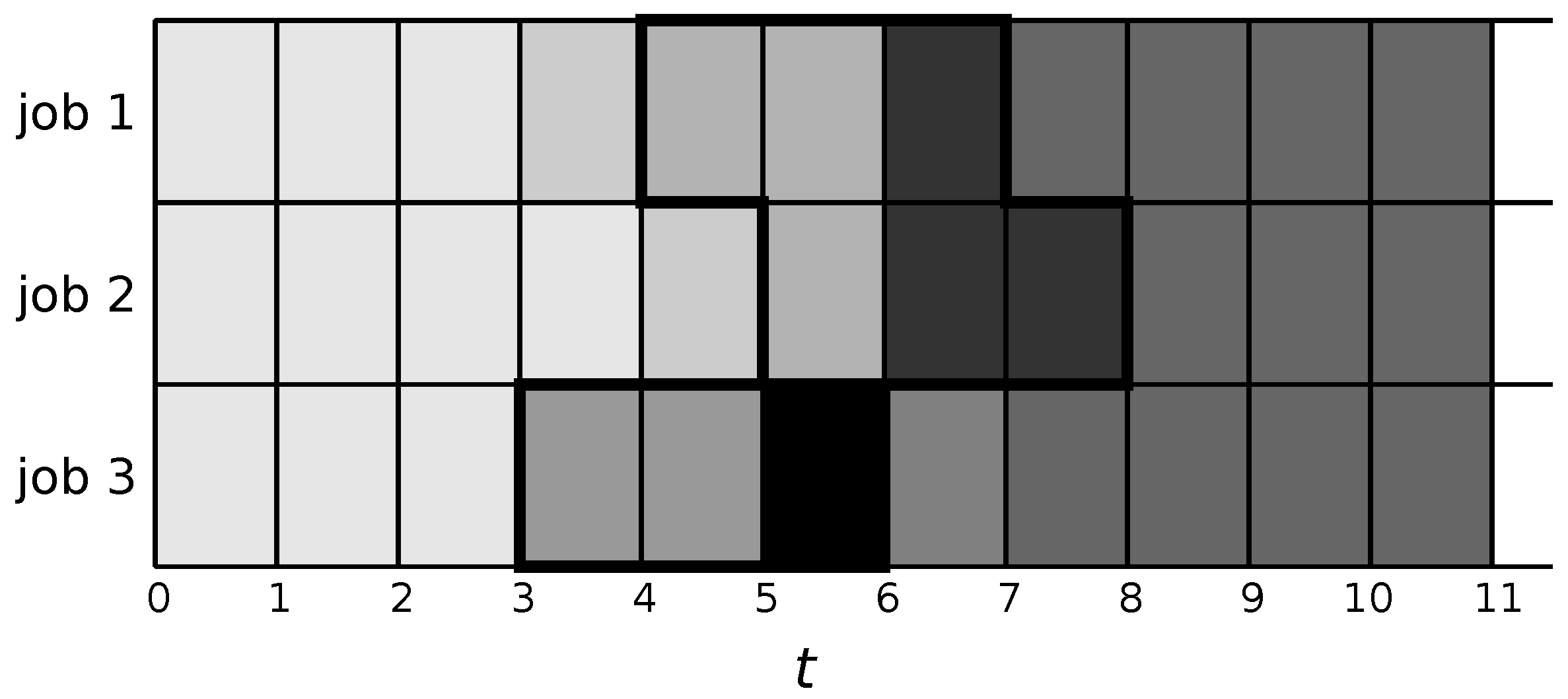
The following example illustrates how partitioning and random splitting in MS is achieved. Figure 2 deals with a simple example instance of the RCJS problem with three jobs that must be executed on the same machine. Moreover, the graphic shows the values of the z-variables of three different solutions, where for each job, each of the three rows of binary values represents the variable values of a solution. Note that these three solutions lead to the set of variables V being partitioned into six sets, as indicated by the background of the cells shaded in different levels of grey. More specifically, the portion corresponding to the example in Figure 2 consists of the following six sets (ordered from the lightest shade of grey to the darkest shade of grey):
The sets from Figure 2 can now be used to generate the restricted MIP, potentially leading to a better solution than the original three solutions used to generate it. However, the sets can be limiting (since there could be very few) and hence random splitting may be used to generate more sets in order to expand the neighbourhood around the current set of solutions that will be searched by the restricted MIP. Figure 3 shows such an example, where the original set was split further (darkest shade) into subsets and , and the original set was split into subsets and (black), that is, with a value 2 for parameter K. Solving the resulting restricted MIP allows for a larger number of solutions and potential improvements. Note, however, that splitting too many times—that is, with a large value of K—can lead to a very complex MIP. For sufficiently large K each set is a singleton and the “restricted” MIP is simply the original problem.
3.1.2. Reasons for Choosing Model 2 in MS
The reasons for choosing Model 2 over Model 1 in the context of MS are as follows. First, general-purpose MIP solvers are more efficient in solving Model 2. Second, the variables of Model 2 adapt better to the way in which variables are split into sets in MS. Attempting the same aggregation using Model 1 (the model defined in Section 2.3) would lead to several inefficiencies. For example, it would only be possible to identify very few partitions, most of which would be disjointed and random splitting would not be effective. By contrast, in Model 2 if multiple solutions include for some variables , this simply means that, in all of the solutions, job j is completed at time t or earlier, even if these solutions differ in exactly when job j is completed. To make this more concrete, consider the example in Figure 2 with the only requirements being that each job is scheduled exactly once. Now, the merge neighbourhood of Model 2 permits any combination of starting times of jobs 1 and 2 at (3,4), (4,5) or (7,8), respectively, combined with job 3 starting at times 3, 6 or 7 for a total of nine possible solutions. By contrast, if we used Model 1 then the only binary patterns generated by the solutions would be (0,0,0), (1,0,0), (0,1,0) and (0,0,1) and the merge search neighbourhood would only include the three original solutions.
3.2. Construct, Solve, Merge and Adapt
Algorithm 2 presents the pseudo-code of the CMSA heuristic for the RCJS problem. The inputs to the algorithms are (1) an RCJS problem instance, (2) the number of solutions constructed per iteration (), (3) the total computational (wall-clock) time (), (4) the wall-clock time limit of the MIP-solver at each iteration (), and (5) the maximum age limit (). The algorithm maintains a set of variables, , which is a subset of the total set of variables in the MIP model, denoted by V. In contrast to MS, CMSA uses Model 1 for the restricted MIP solved at each iteration. In the context of CMSA, a valid solution S to the RCJS problem is a subset of V—that is, . The corresponding solution is obtained by assigning the value 1 to all variables in S and 0 to all variables in . Again, represents the objective function value of solution S.
| Algorithm 2 CMSA for the RCJS Problem. |
|
The algorithm starts by initialising relevant variables and parameters: (1) , where is the subset of variables that should be considered by the restricted MIP, (2) —that is, no best-so-far solution exists, (3) , where is the so-called age value of variable . With this last action, all age values are initialized to zero.
Between Lines 3 and 11, the main algorithm executes. The algorithm runs up to a time limit and, as mentioned earlier, this is one hour of wall-clock time. As in MS, solutions are constructed at each iteration. Remember that the variables contained in a solution S indicate the completion times of every job. As specified earlier, for the purpose of this study, we investigate a constructive heuristic and ACO. Each solution that is found is incorporated in (Line 6) by setting a flag for the associated variables to be free when solving the restricted MIP in function Apply_MIP_Solver(,,) (Line 8). In other words, the restricted MIP is obtained from the original/complete one by only allowing the variables from to take on the value 1. As in the case of MS, solving the restricted MIP is warm-started with the best-so-far solution (if any). The restricted MIP is solved with a time limit of seconds and returns a possibly improved solution . Note that this solution is at least as good as the original seed solution. In Line 9, a solution improving on is accepted as the new best-so-far solution. In Adapt , the age parameter of all variables is incremented, except for those that appear in . If a variable’s age has exceeded , it is removed from . Moreover, its age value is set back to zero after terminating, the best-so-far solution found is output by the algorithm.
3.2.1. Reasons for Choosing Model 1 in CMSA
As mentioned already above, CMSA makes use of Model 1, as defined in Section 2.3, in the context of solving the restricted MIP. This is, indeed, the most natural formulation for CMSA, given that we can exactly specify which variables should take value zero, or should be left free. However, note that it would also be possible to use Model 2 instead. In this case, a range of variables would have to be left free, including the earliest and latest times that a job can be completed. However, we found in preliminary experiments that this results in very long run-times as there are many more open variables, which leads to an inefficient overall procedure.
3.2.2. CMSA Intuition
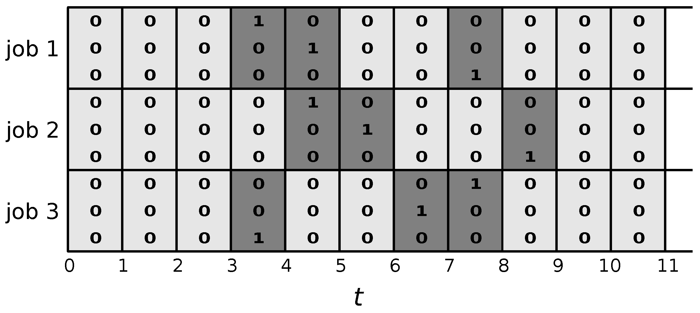
Figure 4 shows the same solutions as in Figure 2. However, the variable values displayed in this graphic are now according to Model 1—that is, only the variables corresponding to the finishing times of the three jobs in the three solutions take value one. All other variables take value zero. When the restricted MIP is solved, these are the only times that will be allowed for the jobs to complete.
A size of the search space spanned by the restricted MIP in CMSA is controlled by the number of solutions generated at each iteration () and by the degree of determinism used for generating these solutions. For example, the higher and the lower the degree of determinism, the larger the search space of the restricted MIP. Similar ideas to those of random splitting could also be used within CMSA, where more variables could be freed than only those that appear in the solution pool. This may be useful for problems which require solving an MIP with a large number of variables to find better solutions. However, the original implementation [19] did not use such a mechanism and hence we do not explore it here.
3.3. Parallel Ant Colony Optimisation
An ACO model for the RCJS was originally proposed by [27]. This approach was extended to a parallel method in a multi-core shared memory architecture by [29]. For the sake of completeness, the details of the ACO implementation are provided here.
As in the case of the constructive heuristic, a solution in the ACO model is represented by a permutation of all tasks (). This is because there are potentially too many parameters if the ACO model is defined to explicitly learn the finishing times of the tasks. Given a permutation, a serial scheduling heuristic (see [35]) can be used to generate a resource and precedence feasible schedule consisting of finishing times for all tasks in a well-defined way. This is described in Section 3.3.1, below. Moreover, based on the finishing times, the MS/CMSA solutions can be derived. The objective function value of an ACO solution is denoted by .
The pheromone model of our ACO approach is similar to that used by [36]—that is, the set of pheromone values () consist of values that represent the desirability of selecting job j for position i in the permutations to be built. Ant colony system (ACS) [37] is the specific ACO-variant that was implemented.
The ACO algorithm is shown in Algorithm 3. An instance of the problem and the set of pheromone values are provided as input. Additionally, a solution () can be provided as an input which serves the purpose of initially guiding the search towards this solution. If no solution is provided, is initialised to be an empty solution.
| Algorithm 3 ACO for the RCJS Problem. |
|
The main loop of the algorithm at Lines 3–9 runs until a time or iteration limit is exceeded. Within the main loop, a number of solutions () are constructed (ConstructSolution()). Hereby, a permutation is built incrementally from left to right by selecting, at each step, a task for the current position , making use of the pheromone values. Henceforth, denotes the tasks that can be chosen for position i—that is, consists of all tasks not assigned already to an earlier position of . In ACS, a task is selected in one of two ways. A random number is generated and a task is selected deterministically if . That is, task k is chosen for position i of using
Otherwise, a probabilistic selection is used where job k is selected according to
Every time a job k is selected at position i, a local pheromone update is applied:
where is a small value that ensures that a job k may always be selected for position i.
After the construction of solutions, the iteration-best solution is determined (Line 5). This solution is improved by way of local search (Improve()), as discussed in [29]. The global best solution is potentially updated in function Update(): . Then, all pheromone values from are updated using the solution components from in function PheromoneUpdate():
where and Q is a factor introduced to ensure that . The value of the evaporation rate is set at —the same value used in the original study [35].
3.3.1. Scheduling Jobs
Given permutation of all jobs, a resource and precedence feasible solution specifying the start times for every job can be obtained efficiently [23]. This procedure is also called the serial scheduling heuristic.
Jobs are considered in the order in which they appear in the permutation . A job is selected and examined to see if its preceding jobs have been completed. If so, the job is scheduled as early as possible, respecting the resource constraints. If not, the jobs are placed on a waiting list. If it is possible to schedule a job, the waiting list is examined to see if any waiting job can be scheduled. If yes, the waiting job is immediately scheduled (after its preceding job(s)) and the waiting list is re-examined. This repeats until the waiting list is empty or no other job on the waiting list can be scheduled. At this point the algorithm returns to consider the next job from .
3.3.2. Using Parallel ACO within MS and CMSA
As mentioned earlier, parallelization is achieved by running each colony on its own thread, without any information sharing. Since several colonies run concurrently, a larger (total) run-time allowance can be provided to the solution construction components of MS and CMSA. Note that the ACO algorithm may be seeded with a solution (see Algorithm 3). This effectively biases the search process of ACO towards the seeding solution. In the case that this solution is not provided, the ACO algorithm is run without any initial bias. Since the restricted MIPs of MS and CMSA benefit greatly from diversity, one of the colonies is seeded with the current best-so-far solution of MS, respectively CMSA, while the other colonies do not receive any seeding solution (Note, we performed tests where two or more of the colonies were seeded with the best solution. We found that there was no significant difference up to five colonies, after which the solutions were worse. Hence, we chose one colony to be seeded with the best solution).
4. Motivation and Hypotheses
In this section we briefly outline the motivation behind the solution-merging-based approaches and some hypotheses regarding the behaviour of the algorithms that were to be tested informally in the empirical results. There are several interrelated aspects of the algorithms to be investigated and we broadly categorise these by their similarities and differences.
Learning patterns of variable values: Given a population of solutions, both algorithms learn information about patterns of variable values that are likely to occur in any (good) solution. This aspect is similar to other population-based metaheuristics, such as genetic algorithms [38].
The main difference between construct, merge, solve and adapt (CMSA) and Merge search (MS) is that the former focuses on identifying one large set of variables that have a fixed value in good solutions. The remaining set of variables is subject to optimization. MS, on the other hand, looks for aggregations of variables—that is, groups of variables that have a consistent (identical) value within good solutions. However, their specific value is subject to optimization. In the case of MS, very large populations can still lead to a restricted mixed integer program (MIP) with reasonable run-times, since the method uses aggregated variables.
Static heuristic information vs learning: Constructive heuristics, such as greedy heuristics, are typical methods for generating solutions to most scheduling problems and we investigate one such method in this study. However, we are very interested to see if using a more costly learning mechanism can lead to inputs for MS and CMSA, such that their overall performance improves. This aspect is implemented with ant colony optimisation (ACO) in this paper. ACO is more likely to find good regions in the search space. However, running an ACO algorithm is computationally much more expensive than generating a single solution. We aim to identify if this trade-off is beneficial.
Strong bias towards improvements over time: Both methods generate, at each iteration, restricted MIPs whose search space includes all the solutions that contributed to the definition of the MIPs, in addition to combinations of those. Hence, the solution generated as a result of the merge step is at least as good as the best one of the input solutions. The question here in the absence of any hill climbing mechanism, relying only on random solution generation is sufficient to prevent these methods from becoming stuck in local optima.
Population size: As with any neighbourhood search or population based approach we expect there to be a trade-off between diversification and intensification, which—in MS and CMSA—is essentially controlled both by the size and by the diversity of the populations used in each merge step. Given the difference in the merge operations, we can expect the best-working population size to be somewhat different for the two algorithms. In fact, we expect it to be smaller for CMSA as compared to MS.
Random splitting in MS: This mechanism is nearly equivalent to increasing the search space by throwing in more solutions, except that (a) it is faster than generating more solutions and (b) it provides some extra flexibility that might be hard to achieve in problems that are very tightly constrained and, hence, have relatively few and quite varied solutions.
Neighbourhood size: For a given set of input solutions, we expect the restricted MIPs in CMSA to have a larger search space in the neighbourhood of the input solutions than the MIPs in MS (with random splitting based on ) leading to better solutions from the merge step, but leading to longer computation times for each iteration. This aspect can change substantially with an increasing value of K.
5. Experiments and Results
C++ was used to implement the algorithms, and the implementations were compiled with GCC-5.2.0. The mixed integer programming (MIP) component was implemented using Gurobi 8.0.0 [39] and the parallel ant colony optimisation (ACO) component using OpenMP [40]. The experiments were conducted on Monash University’s Campus Cluster with nodes of 24 cores and 256 GB RAM. Each physical core consisted of two hyper-threaded cores with Intel Xeon E5-2680 v3 2.5GHz, 30M Cache, 9.60GT/s QPI, Turbo, HT, 12C/24T (120W).
The experiments were conducted on a dataset from [23]. This dataset consists of problem instances with 3 to 20 machines, with three instances per machine size. There is an average of jobs per machine. This means that an instance with 3 machines has approximately 32 jobs. Further details of the problem instances, and how the job characteristics (processing times, release times, weights, etc.) were determined, can be obtained from the original study.
To compare against existing methods for resource constrained job scheduling (RCJS), we ran column generation and ACO (CGACO) of [28], column generation and differential evolution (CGDELS) of [41], the MIP (Model 2—which is most efficient), column generation (CG) on its own and parallel ACO. The results for the MIP, CG and ACO are presented in Appendix D and are not discussed in the following sections as they prove not to be competitive.
Thirty runs per instance were conducted and each run was allowed one hour of wall-clock time. Based on the results obtained in Section 5.4, 15 cores were allowed for each run (that is, Gurobi uses 15 cores when solving the involved MIPs and the ACO component is run with ). To allow a fair comparison with CGACO and CGDELS, the same algorithm was run on the same infrastructure using 15 cores per run. The parameter settings for the individual merge search (MS) and construct, merge, solve and adapt (CMSA) runs were obtained by systematic testing (see Appendix B and Appendix C). The detailed results are provided in the following sections. The parameter settings for each individual ACO colony were the same as those used in [27,29]: , and .
The result tables presented in the next sections are in the following format. The first column shows the name of the problem instance (e.g., 3–5 is an instance with 3 machines and id 5). For each algorithm we report the value of the best solution found in 25 runs (Best), the average solution quality across 25 runs (Mean), and the corresponding standard deviation (). The number of performed iterations, as an average across the 25 runs, is also provided (). The best results in each table are marked in boldface. Moreover, all statistically significant results, obtained by conducting a pairwise t-test and using a confidence interval of 95%, are marked in italics.
5.1. Study of Merge Search
MS relies on a “good” diverse pool of solutions to perform well. There are two approaches one could take to this: (1) simply constructing a diversity of random solutions as quickly as possible, or (2) searching for a population of good solutions in the neighbourhood of the best found. In the literature, CMSA takes the first approach while MS takes the second. We conducted experiments with a constructive heuristic (see Appendix A) and ACO (Table 1) for the first and second approaches, respectively. The parameters for MS are the MIP time limit ( = 120 s), the number of ACO iterations (5000) and the value of the random splitting parameter (). Parameter values were chosen according to parameter tuning experiments (see Appendix B).
We see that using ACO within MS (called MS-ACO) is far superior to using the constructive heuristic. ACO provides a distinct advantage across all problem instances, which must be due to the fact that the solutions for the generation of the restricted MIPs are very good, due to the computation time invested in learning (made efficient via parallelization). Not surprisingly, the number of iterations performed by MS-Heur is much larger than that by MS-ACO, within the given time limits. This is mainly due to the fact that the solution construction in MS-ACO lasts more than 5000 times longer than that of MS-Heur. This demonstrates conclusively that, for MS, having a set of good solutions clustered around the best known solution is better than a diverse set of randomly generated solutions. Next, we will test whether the same conclusion holds for CMSA.
5.2. Study of CMSA
As with MS, we can also use the constructive heuristic or ACO (labelled CMSA-ACO) within CMSA to generate solutions. The parameters of CMSA, including the time limit for solving the restricted MIPs ( = 120 s), ACO iterations (5000) and the maximum age limit ( = 5, for instances with 8 or fewer machines and = 3, for instances with 9 or more machines) were determined as a result of the parameter tuning experiments (See Appendix C). As in the case of MS, we can observe that ACO (Table 2) provides a distinct advantage across all problem instances.
Overall, constructing the solutions with ACO seems to help the iterative process of CMSA to focus on very good regions of the search space. For RCJS, the results demonstrate that, irrespective of the details of the merge method, solution merging works much better as an additional step to improve results in a population based metaheuristics than as the main solution intensification method on its own.
In contrast to the case of MS-Heur and MS-ACO, it is interesting to observe that the number of iterations performed by CMSA-Heur is of the same order of magnitude as that of CMSA-ACO. Even though CMSA-Heur usually performs more iterations than CMSA-ACO, in a small number of cases—concerning the small problem instances with up to four machines, in addition to instance 5–21—there are fewer iterations conducted by CMSA-Heur. Investigating this more closely by examining the restricted MIP models generated within the CMSA versions, we found that the constructive heuristic provides slightly more diversity as several ACO colonies converge to the same solution. In the context of CMSA, this leads to more variables in the restricted MIP and hence to a significant increase in MIP solving time. This increase in time for the merge step consumes most of the time saved in the faster time of the constructive heuristic compared to ACO.
5.3. Comparing CGACO, CGDELS, BRKGA, MS and CMSA
We now investigate how the best versions of MS and CMSA (both using ACO for generating solutions) perform against the current state-of-the-art methods for the RCJS problem. Reference [28] showed that the CGACO hybrid is very effective, while [41] (CGDELS) and [42] (BRKGA) are current state-of-the-art approaches. For a direct comparison, we run these methods, allowing the same computational resources with the same run time limits. The results are shown in Table 3.
The comparison here is with respect to upper bounds, as we are only interested in feasible solutions in this study. We see that within one hour of wall clock time, CGACO is always outperformed by MS and CMSA. With increasing problem size, the differences are accentuated. The comparison with CGDELS shows that MS and CMSA perform better on 20/36 problem instances. For the smallest problem instances (3–5 machines), MS and/or CMSA are best. The results are split for small to medium-sized instances (6–9 machines) followed by a clear advantage of CGDELS for medium to large sized instances (9–12 machines). For the largest instances, CMSA regains the advantage. The best performing method is clearly BRKGA, but for the small to medium instances, MS and CMSA are able to find better solutions (on 11/36 problem instances).
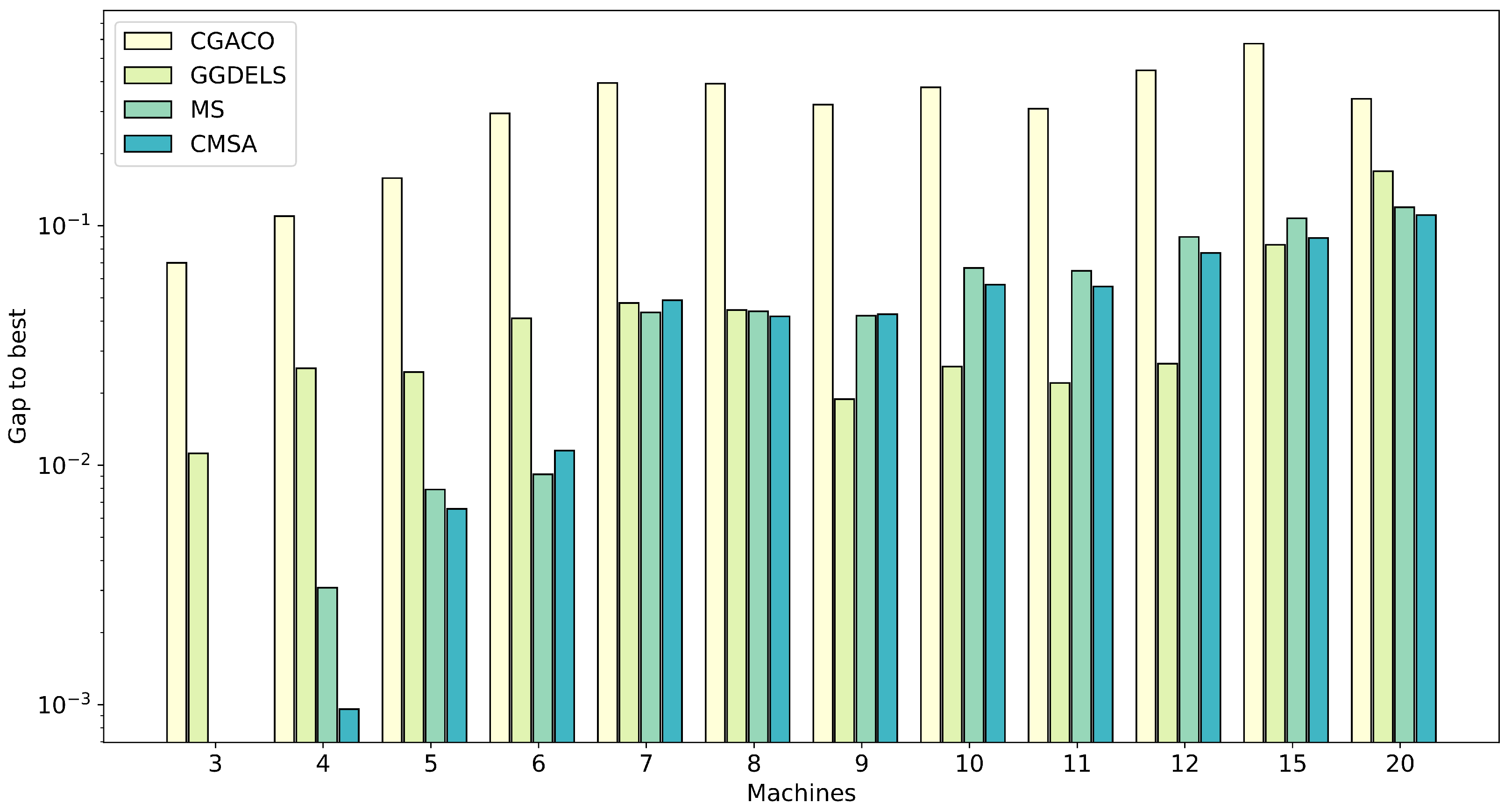
Comparing MS and CMSA, we can observe that both algorithms are very effective in finding good solutions within the given time limit. MS finds best solutions (best in 17 out of 36 instances) for nearly half of the instances. This is mainly the case for the problem instance of small and medium sizes (up to 10 machines). CMSA, on the other hand, is very effective for small instances (up to 5 machines) and then more effective again on the larger instances (≥10 machines), finding the best solution in 26 out of 36 cases. For instances of 10 machines and beyond, CMSA is clearly the best-performing method. This aspect is also summarized in Figure 5, where, for each method, the average performance across instances on the same number of machines is plotted, with respect to the percentage difference to the best performance. CGACO is always outperformed by all other methods. CGDELS performs the best for problem instances with 9, 10, 11 and 12 machines, and for the remaining machine sizes (except 15 machines), MS and CMSA are best. The case with 15 machines is interesting because CMSA or MS are generally more effective, but CGDELS is overwhelmingly more effective in one instance (15–2), thereby skewing the average. We see that while MS is effective for instances with a low number of machines and CMSA is more effective for the larger instances.
Comparing MS and CMSA in terms of iterations (Table 1 and Table 2) show that there are many more iterations performed by MS for problem instances of small and medium size (up to 8 machines). This is due to very small restricted MIPs being generated at each iteration in MS, which—in turn—is due to the large amount of overlap among the generated solutions. MS-ACO and CMSA-ACO are much closer to each other in terms of the number of iterations performed, but we see that CMSA-ACO generally performs fewer iterations. This is again due to the larger solving times of the MIPs and validates our hypothesis that the solution space induced by CMSA is larger when MS has very few sets.
The above experiments demonstrate the efficacy of MS-ACO and CMSA-ACO compared to the state-of-the-art method for RCJS. It has been previously shown [28] that ACO on its own is not very effective for this problem. However, so far it remains unclear how much of the improvement in solution quality can be attributed to solution merging and to the ACO component of the search. To further understand this aspect, we measured the relative contribution of the merge step of MS and CMSA in the MS/CMSA hybrid—that is, the contribution obtained by solving the restricted MIPs. Table 4 shows these results as the percentage contribution of the merge step (MS/CMSA-MIP) relative to the total improvement (MS/CMSA+ACO). For example, suppose we have the following steps in one run of MS-ACO:
- Solve MIP: starting objective 5000, final objective 4500: = = 10.0%.
- Solve ACO: objective 4200.
- Solve MIP: starting objective 4200, final objective 4000: = = 4.0%.
- Solve ACO: objective 4000.
- Solve MIP: starting objective 4000, final objective 3500: = = 10.0%.
The contribution of MS-MIP is and MS+ACO is . This calculation shows that, in the example, the MIP component plays a more substantial role than the ACO component in improving the solutions.
Table 4 provides the complete set of results for this solution improvement analysis. We see that, for a number of instances, the contributions of the merge step and ACO are similar. However, the cases in which the contribution of the merge step is more substantial concern the smaller and the medium-sized instances (e.g., 5–7 and 6–28), whereas ACO contributes more substantially in the context of the larger instances (e.g., with 12, 15, and 20 machines). This is not surprising, as ACO actually consumes the majority of the runtime of the algorithm in those cases, in which only a small number of iterations can be completed within the time limit.
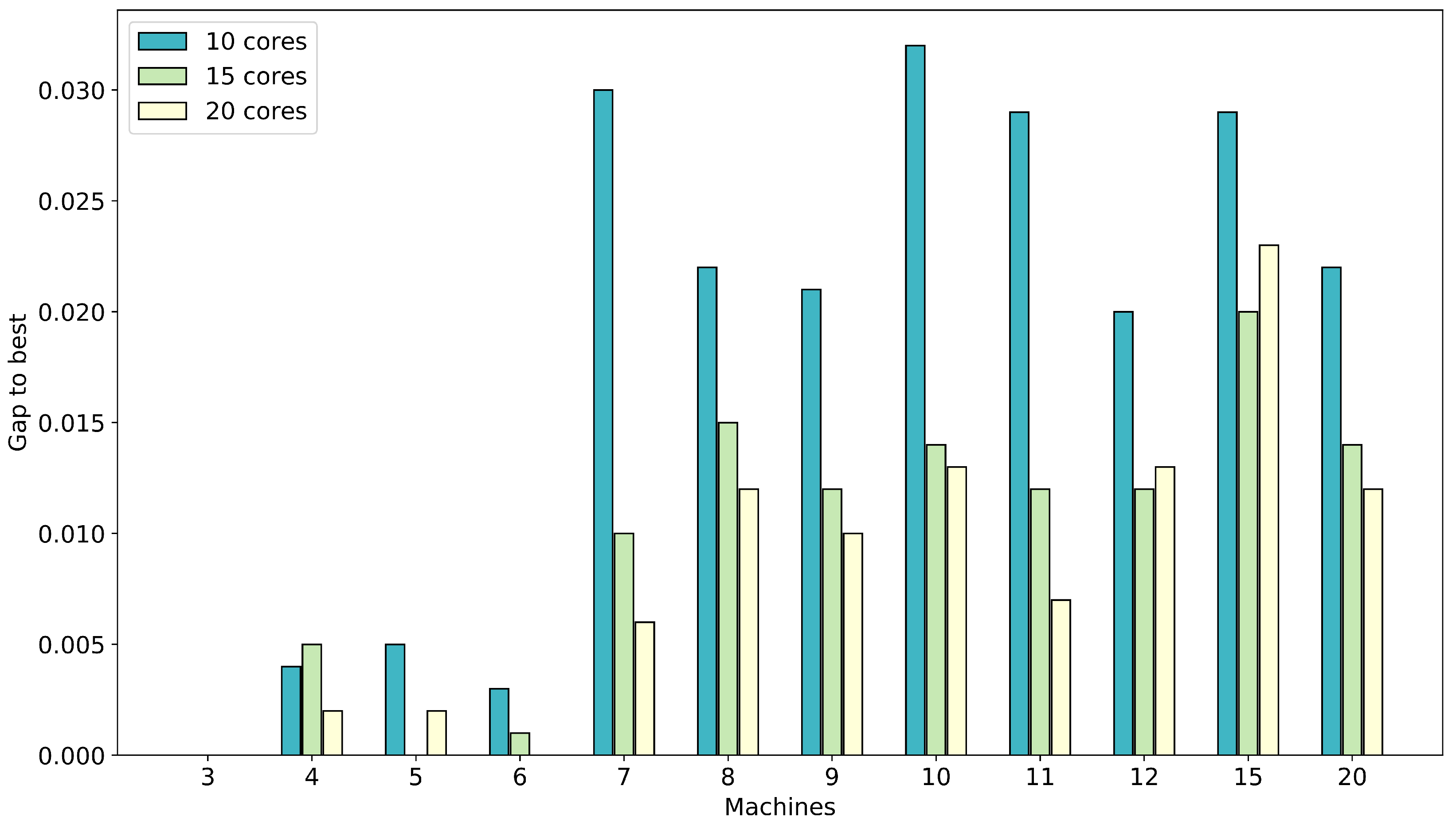
5.4. Study Concerning the Number of Cores Used
Remember that the number of allowed cores influences two algorithmic components: (1) the ACO component, where the number of cores corresponds to the number of colonies and (2) the solution of the restricted MIPs (which is generally more efficient when more cores are available). However, with a growing number of allowed cores, the restricted MIPs become more and more complex, due to being based on more and more solutions. In any case, the number of allowed cores should make a significant difference to the performance of both MS-ACO and CMSA-ACO.
The results are presented in Figure 6 and Figure 7. The figures show the average over all instances with the same number of machines of 25 runs for the gap to the best solution found by any of the methods. The results for MS-ACO show that using 15 or 20 cores is preferable compared to using only 10 cores. The difference between 15 and 20 cores is small with a slight advantage using 20 cores.
As mentioned already above, the diversity of the solutions generated when using 20 cores leads to large restricted MIPs (many more variables) to be solved, which can be very time consuming and even very inefficient. Hence, on occasion, 15 cores are preferable to 20 cores. Compared to using 10 cores, using 15 or 20 cores cores provides sufficient diversity leading to good areas of the search space for the restricted MIPs within the 120 s time limit.
The results for CMSA-ACO show that overall the use of 15 or 20 cores is preferable over only using 10 cores. In CMSA-ACO, several instances are solved more efficiently with 20 cores. Though, for the large instances (10 or more machines), the use of 15 cores is most effective. For CMSA the effect of increased number of solutions on increasing the size and complexity of the restricted MIP used in the merge step is even more pronounced than in MS. Hence, overall the use of 15 cores proves to be most effective.
The conclusion of this comparison is that, while solution merging benefits from having a number of different solutions available, a too large pool of solutions can also have a detrimental effect. For RCJS, using 15 solutions is generally the best option irrespective of the type of merge step used (MS vs. CMSA). To better understand the effect of the alternative solution merging approaches, we next test these using exactly the same pools of solutions.
5.5. Comparing MS and CMSA Using the Same Solution Pool
To remove the randomness associated with the generation of a population of solutions, we investigated the alternative merge steps of MS and CMSA using the same solution pool. For this direct comparison we carried out just one algorithm iteration for each instance. The solutions were obtained using ACO, using the same seed—that is, leading to exactly the same solutions available for generating the MIPs of both methods. The time limit provided for solving the restricted MIPs was again 120 s. Random splitting in MS-ACO was set as before to , while the age limit in CMSA-ACO had no effect in this case.
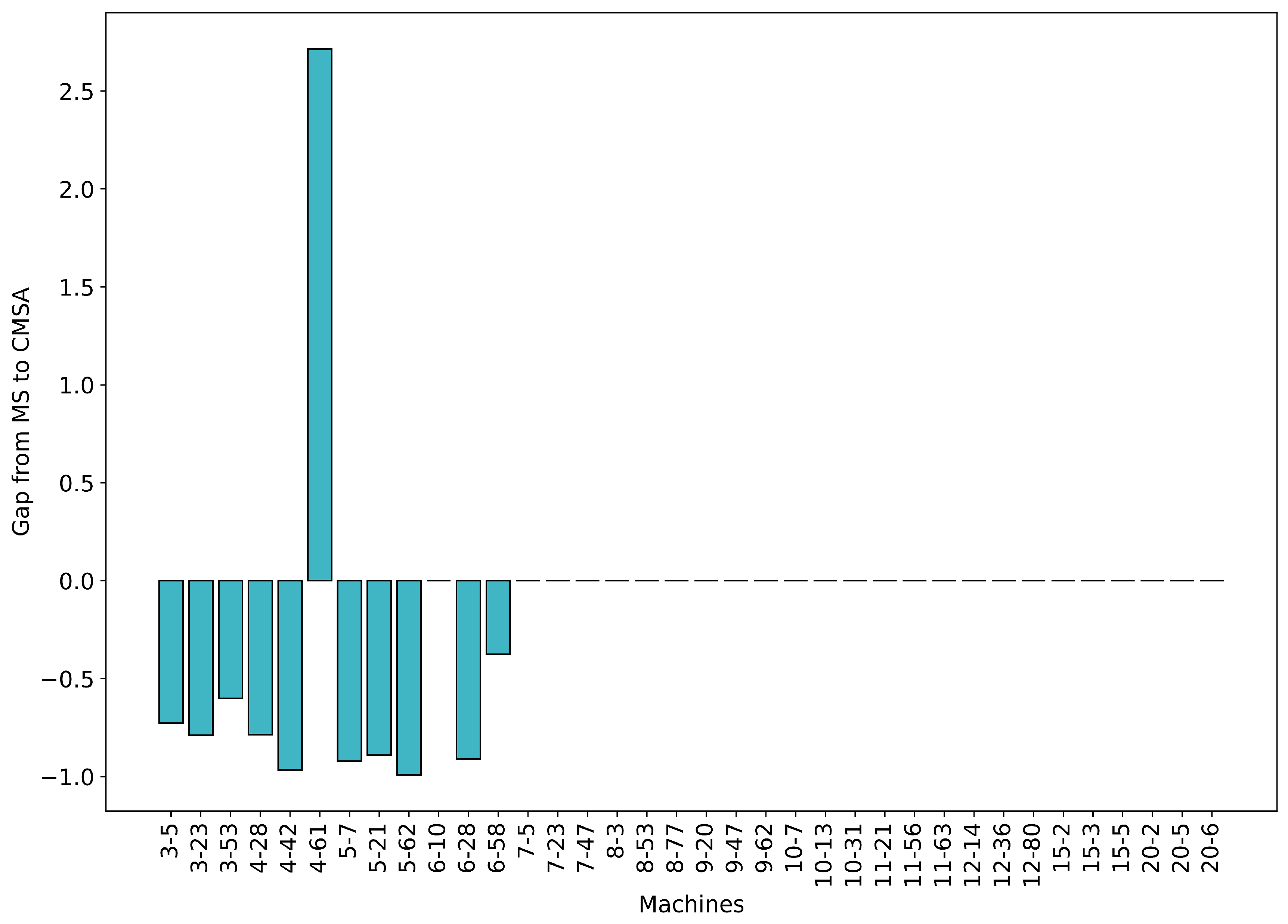
With increasing neighbourhood size, the quality of the solution that can be found in this neighbourhood can be expected to improve. Hence, we use the solution quality as a proxy for the size of the space searched by the MIP subproblems in the two algorithms. Figure 8 shows the gap () or difference in performance (in percent) after one algorithm iteration.
A positive value indicates that CMSA-ACO performed better than MS-ACO, whereas a negative value means the opposite. We see that CMSA-ACO is generally more effective for smaller problems, but this difference reduces in the context of the larger problems, where sometimes MS-ACO can be more effective.
Figure 9 shows a similar comparison, as in Figure 8, but instead considers the time required to solve the restricted MIPs. We see that, for small problems, MS-ACO is a lot faster (except, for instance, 4–61). This further validates the hypothesis that the CMSA-ACO solution space is larger than that of MS-ACO. From seven machines onwards, the MIP-solving exhausts the time limit both in MS-ACO and in CMSA-ACO, hence we see no difference.
6. Discussion
From the experiments conducted, we make the following observations regarding the use of solution merging in the context of heuristic search for the RCJS problem. Both MS and CMSA are more effective when the populations contain solutions from good regions of the search space. While good solutions can be found with heuristics, the results show that the learning mechanism of ACO is critical to the performance of both algorithms. Despite ACO requiring substantially more computational effort, the quality of the solutions used to build the restricted MIPs are vital to the performance of the overall algorithm. This contrasts with the way CMSA was originally proposed using a simple randomised heuristic to generate a pool of solutions.
Both algorithms are very effective and achieve almost the same performance on the smallest problem instances. MS is more effective for medium-size problem instances, whereas CMSA is more effective for the large instances. A key aspect of this is that the solutions generated by ACO are often very good for the problem instances of small and medium size. Thus, the smaller search space of the restricted MIPs in MS, achieved through aggregating variables, allows solving the MIPs much more quickly than in CMSA. However, for the large problem instances, the restricted MIPs in CMSA are more diverse, and hence enable the algorithm to find better quality solutions. Comparing with CGACO, MS and CMSA perform significantly better across all problem instances given the run-time limits.
Given the stopping criteria of one hour of wall-clock time, a large amount of random splitting in MS does not seem beneficial. In fact, the time limit for solving the restricted MIPs (120 s) is too low for solving the increasingly large-scale restricted MIPs obtained from increasing the amount of random splitting (even in the context of problem instances with eight machines, for example). However, increasing this time limit does not prove useful, because more and more of the total computational allowance will be spent on solving fewer and fewer restricted MIPs (leading to fewer algorithm iterations) without necessarily finding improving solutions.
As we hypothesized (Section 4), the way of generating the restricted MIPs in CMSA leads to a larger search space when compared to that of MS. This is validated by the run-times: the restricted MIPs of CMSA usually take longer to be solved than the restricted MIPs of MS (if the 120 s time limit is not exhausted).
Analysing the parallel computing aspect, we were able to observe that—with a total wall-clock time limit of one hour—using 15 cores leads to the best results for both MS and CMSA. Parallel computing is particularly useful when using a learning mechanism such as ACO, where more computational effort is needed to achieve good diverse solutions. However, with too many cores (20), the performance of both methods generally drops. This is because the mechanism for utilising the additional cores results in a larger, more diverse set of solutions. CMSA in particular is severely affected for the large problem instances, where often the process of trying to solve the restricted MIPs is unable to find improvements over the seeding solutions.
Finally, we would like to remark that, in the context of a discrete time MIP formulation of a scheduling problem with a minimum Makespan objective, the restricted MIP could never produce any solution better than the best of the input solutions. This is because improvements in the objective function are limited to values available in the inputs. Hence, an alternative MIP modelling approach should be considered in these cases—for example, based on the order of the jobs (sequencing) without any fixed completing times. This might even be beneficial for the problem considered in this work. Investigating this effect of solution representation for solution merging of RCJS is beyond the scope of the current work, but represents a promising avenue for future research.
7. Conclusions
This study investigates the efficacy of two population-based matheuristics—Merge search (MS) and construct, merge, solve & adapt (CMSA)—for solving resource constrained job scheduling (RCJS). Both methods are shown to be more effective when hybridized with a learning mechanism—i.e., ant colony optimisation (ACO). Furthermore, the whole framework is parallelized in a multi-core shared memory architecture, leading to large gains in run-time. We find that both hybrids are overall more effective than both the individual methods on their own, and better than previous attempts to combine ACO with integer programming, which used column generation and Lagrangian relaxation in combination with ACO. Furthermore, MS and CMSA are competitive with the state-of-the-art hybrid of column generation and differential evolution, especially outperforming this method on small-medium and large problem instances. Comparing MS and CMSA, we see that both methods easily solve small problems (up to five machines), while MS is more effective for medium-sized problem instances (up to eight machines) and CMSA for large problem instances (starting from 11 machines).
We investigate in detail several aspects of the algorithms, including their parallel components, the search spaces considered at each iteration, and algorithm specific components (e.g., random splitting in MS). We find that parallel ACO is very important for identifying good areas of the search space, within which MS and CMSA can very efficiently find improving solutions. The search spaces considered by CMSA at each iteration are typically larger than those of MS, which is advantageous for large problem instances but generally disadvantageous for problem instances of medium size.
Future Work
The generic nature of MS and CMSA mean that they can be applied to a wide range of problems. There are two main requirements: (1) a method of generating good (and diverse) feasible solutions and (2) an efficient model for an exact approach. Given these aspects, both algorithms are capable of being applied to other problems with little overhead and the promise of good results. Individually, they are already proven on some problems [18,19,20,21], with more studies having been conducted with CMSA. Hence, there are several possibilities of applying both approaches to different problems. We are currently investigating the efficacy of MS and CMSA on the resource constrained project scheduling maximising the net present value [33,43,44,45].
The parallelisation is effective for both methods. Extending this aspect to a message passing interface framework [46] can be of great potential. In particular, running multiple MSs or CMSAs concurrently and passing (good) solutions between the nodes could lead to the possibility of exploring much larger search spaces. We are currently investigating a parallel MS approach for open pit mining [47,48] with promising preliminary results.
We have briefly discussed the possibility of investigating additional mixed integer programming (MIP) models for their use in MS and CMSA (Section 6). As we pointed out, a sequence-based formulation could be very effective for the RCJS problem. Moreover, given that several problems can be modelled by similar sequence-based formulations, it can be expected that this aspect can transfer to those problems in a straightforward manner. Furthermore, different solvers could be attempted instead of the MIP solvers. For example, for very tightly constrained problems, constraint programming could prove very useful.
The similarities between MS and CMSA suggest that both algorithms can be combined into one high-level algorithm as a generic procedure for solving combinatorial optimisation problems. This approach combines the relative strengths of both methods and can prove to be very beneficial on a wide range of applications. For example, a straightforward extension to CMSA is to incorporate random splitting of the search space, and conversely, the age parameter could be incorporated in MS. In fact, this method can be included within state-of-the-art commercial solvers to provide good heuristic solutions during the exploration of the branch and bound search tree.
Finally, note that computational intelligence techniques other than the ones utilized and studied in this work might be successfully used to solve the considered problem. For a recent overview on alternative techniques with a special focus on bio-inspired algorithms we refer the interested reader to [49].
Author Contributions
Methodology, D.T., C.B. and A.T.E.; Writing—original draft, D.T.; Writing—review and editing, D.T., C.B. and A.T.E. All authors have read and agreed to the published version of the manuscript.
Funding
This work was supported by project CI-SUSTAIN funded by the Spanish Ministry of Science and Innovation (PID2019-6GB-I00).
Acknowledgments
We acknowledge administrative and technical support by Deakin University (Australia), the Spanish National Research Council (CSIC), and Monash University (Australia).
Conflicts of Interest
The authors declare no conflict of interest. The funders had no role in the design of the study; in the collection, analyses, or interpretation of data; in the writing of the manuscript, or in the decision to publish the results.
Abbreviations
| MIP | Mixed Integer Program |
| CMSA | Construct, Solve, Merge and Adapt |
| MS | Merge search |
| ACO | Ant Colony Optimisation |
| RCJS | Resource Constrained Job Scheduling |
| TWT | Total Weighted Tardiness |
| , , | The set of jobs, machines and precedences, respectively |
| Maximum available resource | |
| The time horizon | |
| r, p, d, w, g | The release time, processing time, due time, weight and resource consumption of a job, respectively |
| c | Completion time of a job |
| s, u | Variables that represent start and completion time in the Network Flow model |
| y | Variable to include arcs in the Network Flow model |
| x | Variable that represents completion time of a job in MIP model 1 |
| z | Variable that represents completion time of a job in MIP model 2 |
| CMSA-Heur | CMSA with constructive heuristic |
| MS-Heur | Merge search with constructive heuristic |
| CMSA-ACO | CMSA ACO |
| MS-ACO | Merge search with ACO |
| BRKGA | Biased Random Key Genetic Algorithm |
| CGACO | Column Generation and ACO |
| CGDELS | Column Generation, Differential Evolution and Local Search |
| A solution represented by a permutation of jobs | |
| The iteration best solution | |
| The global best solution | |
| The pheromone trails | |
| Number of solutions to be constructed per iteration | |
| TWT of solution | |
| Pheromone value | |
| Learning rate |
Appendix A. Construction Heuristic
Using a constructive heuristic (in a probabilistic way) is one of the options of generating solutions at each iteration. The constructive heuristic that we developed builds a sequence of all jobs from left to right. For that purpose it starts with an initially empty sequence . At each construction step it chooses exactly one of the so-far unscheduled jobs, and it appends this job to . Henceforth, let be the set of jobs that are already scheduled with respect to a partial sequence . For the technical description of the heuristic, let .
Note that is a crude upper bound for the Makespan of any feasible solution. Moreover, let be the set of jobs that—according to the precedence constraints in —must be executed before j, and let be the subset of jobs that must be processed on machine , . Furthermore, given a partial solution , let be the sum of the already consumed resource at time t.
Given a partial sequence , the set of feasible jobs—that is, the set of jobs from which the next job to be scheduled can be chosen—is defined as follows: . In words, the set of feasible jobs consists of those jobs that (1) are not scheduled yet and (2) whose predecessors with respect to are already scheduled. A time step is a feasible starting time for a job , if and only if
- , for all ;
- , for all (remember that refers to the machine on which job j must be processed);
- , for all .
Here, is the set of feasible starting times for a job and the earliest starting time is defined as . Finally, for choosing a feasible job at each construction step, the jobs from are ordered in the following way. First, a job j has priority over a job k, if . In the case of a tie, job j has priority over job k if . Finally, in the case of a further tie, job j has priority over job k if . If there is still a tie, the order between j and k is randomly chosen. The jobs from are ordered in this way, and this job order is stored in sequence . The first job in is then chosen to be scheduled next. A pseudo-code of the heuristic is provided in Algorithm A1.
Finally, note that a solution constructed by the heuristic can be easily transformed into a Merge search (MS) (respectively, construct, merge, solve and adapt (CMSA)) solution. This is because the heuristic derives starting times for all jobs. The finishing time of each job is calculated by adding its processing time to its starting time. The corresponding variable values of both mixed integer programming (MIP) models can then be derived on the basis of the finishing times.
This heuristic is used in a probabilistic way, as follows. Instead of choosing, at each construction step, the first job from and appending it to , the following procedure is applied. First, a random number is produced. If , the first job from is chosen and appended to . Hereby, is a parameter which we set to value Y for all experiments. Otherwise, the first jobs from are placed into a candidate list, and one of these candidates is chosen uniformly at random and appended to .
| Algorithm A1 Constructive Heuristic. |
|
Appendix B. Merge Search Parameter Value Selection
The Merge search (MS) parameters of interest are the mixed integer program (MIP), time limit (120 and 300 s), the number of iterations in ant colony optimisation (ACO) (500, 1000, 2000 and 5000 iterations) and the number of random sets to split into (2, 4 and 8 sets) (Note that a larger number of split sets implies more diversity, especially since the sets are obtained randomly.). Ten runs per instance were conducted and all runs were conducted for 30 min with 10 cores (The number of cores is also a parameter of interest, but these experiments are conducted in Section 5.4 instead). The results are presented in Table A1. For each parameter of interest, the results are averaged across the results obtained with all values of all the other parameters.
Regarding the MIP time limit, we see that, overall, 120 s is preferable, particularly for eight machines or more. For four and six machines, there are not many differences in the results, but 300 s is slightly preferable for six machines.
The results concerning the number of iterations in ACO are straightforward, with a setting of 5000 iterations providing the best average results across all machines. This suggests that a higher number of ACO iterations could be considered. However, for the 20 machine problem instances, only four iterations of MS complete with 5000 iterations. More ACO iterations will cause—in these cases—that the MS component does not contribute significantly to the final solutions.
The amount of random splitting is almost independent of machine size. Marginally, the smallest number of sets is most beneficial (three out of six problem instances).

Table A1.
The results of experiments conducted to determine which set of parameter values lead to the best solutions for MS. For each parameter, the results are averaged across the results obtained by the settings of all other parameters.
Table A1.
The results of experiments conducted to determine which set of parameter values lead to the best solutions for MS. For each parameter, the results are averaged across the results obtained by the settings of all other parameters.
| Machines | ||||||
|---|---|---|---|---|---|---|
| 4 | 6 | 8 | 10 | 12 | 20 | |
| ACO Iter. | ||||||
| 500 | 66.76 | 240.34 | 790.28 | 703.33 | 2729.48 | 9700.10 |
| 1000 | 66.73 | 239.38 | 727.79 | 671.92 | 2636.11 | 9631.67 |
| 2000 | 66.73 | 238.90 | 692.31 | 644.35 | 2546.22 | 9411.80 |
| 5000 | 66.73 | 238.68 | 670.24 | 633.83 | 2454.07 | 9026.49 |
| MIP Time | ||||||
| 120 | 66.73 | 238.75 | 665.19 | 633.44 | 2444.98 | 9013.80 |
| 300 | 66.73 | 238.60 | 675.29 | 634.23 | 2463.16 | 9039.19 |
| Split Sets | ||||||
| 2 | 66.73 | 238.55 | 664.28 | 641.77 | 2441.72 | 9000.46 |
| 4 | 66.73 | 238.73 | 666.12 | 631.06 | 2443.5 | 9015.77 |
| 6 | 66.73 | 238.51 | 665.18 | 627.48 | 2449.73 | 9025.16 |
Appendix C. Construct, Merge, Solve and Adapt Parameter Value Selection
The construct, merge, solve and adapt (CMSA) parameters of interest are the mixed integer program (MIP) time limit (120 and 300 s), the number of iterations in ant colony optimisation (ACO) (500, 1000, 2000 and 5000 iterations) and the maximum age limit (3, 5 and 10). Ten runs per instance were conducted and all runs were conducted for 30 min with 10 cores. The results are presented in Table A2. For each parameter of interest, the results averaged across the results obtained by all possible settings of all the other parameters.
Table A2.
The results of experiments conducted to determine which set of parameter values leads to the best performance of CMSA. For each parameter, the results are averaged across the results of all the settings for all other parameters.
Table A2.
The results of experiments conducted to determine which set of parameter values leads to the best performance of CMSA. For each parameter, the results are averaged across the results of all the settings for all other parameters.
| Machines | ||||||
|---|---|---|---|---|---|---|
| 4 | 6 | 8 | 10 | 12 | 20 | |
| ACO Iter. | ||||||
| 500 | 66.58 | 239.87 | 736.98 | 672.92 | 2656.52 | 9709.08 |
| 1000 | 66.50 | 239.59 | 702.92 | 650.48 | 2568.98 | 9613.49 |
| 2000 | 66.49 | 239.46 | 675.86 | 633.32 | 2489.59 | 9321.38 |
| 5000 | 66.54 | 238.68 | 663.95 | 627.48 | 2431.25 | 8997.16 |
| MIP Time | ||||||
| 120 | 66.62 | 239.22 | 662.23 | 623.99 | 2426.16 | 8976.99 |
| 300 | 66.46 | 238.14 | 665.66 | 630.96 | 2436.35 | 9017.34 |
| Age | ||||||
| 3 | 66.50 | 238.33 | 667.08 | 620.13 | 2423.19 | 8953.46 |
| 5 | 66.27 | 238.40 | 656.76 | 621.92 | 2429.5 | 8986.49 |
| 10 | 66.60 | 237.69 | 662.86 | 629.93 | 2425.78 | 8991.02 |
Regarding the MIP time limit, we see that, overall, 120 s is preferable, particularly for eight machines or more. For four and six machines, 300 s is preferable; however, the results are close here.
The results concerning the number of ACO iterations show that, generally, 5000 iterations provide the best average results across all machines. It is only for the instance with four machines that 2000 iterations works better. However, for these instances, the results are very close across all possible settings. As with MS, more ACO iterations could be considered, but this would lead to very few CMSA iterations being completed within the total time limit.
The results concerning the maximum age parameter are not as clear. A low maximum age (3) seems the best option overall.
Appendix D. Results of the Mixed Integer Program, Column Generation and Ant Colony Optimisation
Table A3 shows the results for the mixed integer program (MIP) (a single run per instance), column generation (CG) on its own CG and parallel ant colony optimisation (ACO) [29]. Since the MIP is deterministic, a single run per instance was conducted. For CG and ACO, which are stochastic, thirty runs per instance were conducted.
Table A3.
MIP, CG and ACO for the RCJS problem. UB is the upper bound; Best is the best solution found across 25 runs; Mean is the average solution quality across 24 runs. The best results are highlighted in boldface.
Table A3.
MIP, CG and ACO for the RCJS problem. UB is the upper bound; Best is the best solution found across 25 runs; Mean is the average solution quality across 24 runs. The best results are highlighted in boldface.
| Instance | MIP | CG | ACO | ||||
|---|---|---|---|---|---|---|---|
| UB | Best | Mean | SD | Best | Mean | SD | |
| 3 - 5 | 505.00 | 558.81 | 558.81 | 0.00 | 505.00 | 505.36 | 1.08 |
| 3 - 23 | 149.07 | 151.91 | 156.90 | 3.27 | 149.07 | 149.07 | 0.00 |
| 3 - 53 | 67.42 | 76.87 | 76.87 | 0.00 | 69.36 | 69.36 | 0.00 |
| 4 - 28 | 23.81 | 27.78 | 27.78 | 0.00 | 23.94 | 24.55 | 1.33 |
| 4 - 42 | 66.73 | 99.46 | 99.46 | 0.00 | 67.64 | 68.19 | 1.47 |
| 4 - 61 | 42.42 | 55.97 | 55.97 | 0.00 | 45.96 | 45.96 | 0.00 |
| 5 - 7 | 315.46 | 291.02 | 291.02 | 0.00 | 255.03 | 272.09 | 12.93 |
| 5 - 21 | 174.83 | 235.72 | 235.72 | 0.00 | 168.63 | 170.63 | 4.36 |
| 5 - 62 | 372.97 | 289.55 | 289.55 | 0.00 | 264.97 | 271.10 | 5.39 |
| 6 - 10 | - | 980.76 | 988.62 | 4.74 | 828.92 | 860.86 | 23.17 |
| 6 - 28 | 213.58 | 276.29 | 278.20 | 1.15 | 218.37 | 226.91 | 4.13 |
| 6 - 58 | 254.07 | 275.50 | 282.17 | 11.06 | 236.05 | 248.55 | 10.43 |
| 7 - 5 | 563.85 | 483.98 | 491.58 | 11.61 | 433.53 | 453.70 | 11.90 |
| 7 - 23 | - | 639.37 | 643.91 | 2.50 | 553.45 | 597.02 | 26.85 |
| 7 - 47 | - | 574.14 | 574.14 | 0.00 | 446.10 | 469.30 | 18.87 |
| 8 - 3 | - | 761.38 | 769.90 | 5.46 | 671.12 | 703.81 | 27.67 |
| 8 - 53 | - | 529.67 | 545.01 | 10.04 | 464.28 | 488.41 | 11.66 |
| 8 - 77 | - | 1408.13 | 1424.62 | 24.39 | 1232.72 | 1291.09 | 30.83 |
| 9 - 20 | - | 1017.12 | 1040.28 | 18.91 | 925.65 | 961.86 | 27.72 |
| 9 - 47 | - | 1416.23 | 1416.23 | 0.00 | 1243.27 | 1275.26 | 27.42 |
| 9 - 62 | - | 1587.65 | 1587.65 | 0.00 | 1455.66 | 1512.09 | 33.61 |
| 10 - 7 | - | 2730.18 | 2779.31 | 37.38 | 2549.46 | 2704.64 | 107.84 |
| 10 - 13 | - | 2446.87 | 2454.69 | 10.28 | 2245.94 | 2302.92 | 39.89 |
| 10 - 31 | - | 679.91 | 679.91 | 0.00 | 611.71 | 643.65 | 25.05 |
| 11 - 21 | - | 1119.51 | 1119.51 | 0.00 | 1008.00 | 1057.38 | 26.02 |
| 11 - 56 | - | 1926.50 | 1956.86 | 17.84 | 1845.93 | 1875.65 | 25.62 |
| 11 - 63 | - | 2209.79 | 2214.59 | 7.96 | 2032.36 | 2092.44 | 47.81 |
| 12 - 14 | - | 1935.00 | 1967.10 | 28.07 | 1830.31 | 1882.37 | 26.23 |
| 12 - 36 | - | 3248.84 | 3275.53 | 15.08 | 3033.78 | 3138.60 | 66.32 |
| 12 - 80 | - | 2683.73 | 2684.36 | 0.38 | 2433.86 | 2495.55 | 61.31 |
| 15 - 2 | - | 4274.77 | 4403.93 | 70.53 | 3961.82 | 4121.60 | 106.77 |
| 15 - 3 | - | 4655.97 | 4775.44 | 146.92 | 4368.66 | 4514.54 | 121.22 |
| 15 - 5 | - | 3799.43 | 3823.09 | 73.36 | 3512.33 | 3618.10 | 67.65 |
| 20 - 2 | - | 9173.91 | 9249.91 | 49.75 | 8788.97 | 8935.63 | 119.47 |
| 20 - 5 | - | 16,033.40 | 16,192.51 | 170.12 | 14,779.80 | 15,050.51 | 137.54 |
| 20 - 6 | - | 8273.11 | 8273.11 | 0.00 | 7865.08 | 8048.25 | 156.97 |
References
- Blum, C.; Roli, A. Metaheuristics in Combinatorial Optimization: Overview and Conceptual Comparison. ACM Comput. Surv. 2003, 35, 268–308. [Google Scholar] [CrossRef]
- Back, T. Evolutionary Algorithms in Theory and Practice: Evolution Strategies, Evolutionary Programming, Genetic Algorithms; Oxford University Press: Oxford, UK, 1996. [Google Scholar]
- Dulebenets, M.A.; Kavoosi, M.; Abioye, O.; Pasha, J. A Self-adaptive Evolutionary Algorithm for the Berth Scheduling Problem: Towards Efficient Parameter Control. Algorithms 2018, 11, 100. [Google Scholar] [CrossRef] [Green Version]
- Slowik, A.; Kwasnicka, H. Nature inspired methods and their industry applications—Swarm intelligence algorithms. IEEE Trans. Ind. Inf. 2017, 14, 1004–1015. [Google Scholar] [CrossRef]
- Anandakumar, H.; Umamaheswari, K. A Bio-inspired Swarm Intelligence Technique for Social Aware Cognitive Radio Handovers. Comput. Electr. Eng. 2018, 71, 925–937. [Google Scholar] [CrossRef]
- Marriott, K.; Stuckey, P. Programming With Constraints; MIT Press: Cambridge, MA, USA, 1998. [Google Scholar]
- Wolsey, L.A. Integer Programming; Wiley-Interscience: New York, NY, USA, 1998. [Google Scholar]
- Fisher, M. The Lagrangian Relaxation Method for Solving Integer Programming Problems. Manag. Sci. 2004, 50, 1861–1871. [Google Scholar] [CrossRef] [Green Version]
- Geoffrion, A.M. Generalized Benders decomposition. J. Optim. Theory Appl. 1972, 10, 237–260. [Google Scholar] [CrossRef]
- Speranza, M.G.; Vercellis, C. Hierarchical Models for Multi-project Planning and Scheduling. Eur. J. Oper. Res. 1993, 64, 312–325. [Google Scholar] [CrossRef]
- Pisinger, D.; Ropke, S. Large Neighborhood Search. In Handbook of Metaheuristics; Gendreau, M., Potvin, J.Y., Eds.; Springer US: Boston, MA, USA, 2010; pp. 399–419. [Google Scholar]
- Boschetti, M.A.; Maniezzo, V.; Roffilli, M.; Bolufé Röhler, A. Matheuristics: Optimization, Simulation and Control. In Hybrid Metaheuristics; Blesa, M.J., Blum, C., Di Gaspero, L., Roli, A., Sampels, M., Schaerf, A., Eds.; Springer: Berlin/Heidelberg, Germany, 2009; pp. 171–177. [Google Scholar]
- Archetti, C.; Speranza, M.G. A Survey on Matheuristics for Routing Problems. EURO J. Comput. Optim. 2014, 2, 223–246. [Google Scholar] [CrossRef] [Green Version]
- DellaCroce, F.; Salassa, F. A Variable Neighborhood Search based Matheuristic for Nurse Rostering Problems. Ann. Oper. Res. 2014, 218, 185–199. [Google Scholar] [CrossRef]
- Brouer, B.D.; Desaulniers, G.; Pisinger, D. A Matheuristic for the Liner Shipping Network Design Problem. Transp. Res. Part E Logist. Transp. Rev. 2014, 72, 42–59. [Google Scholar] [CrossRef] [Green Version]
- Brech, C.H.; Ernst, A.T.; Kolisch, R. Scheduling Medical Residents’ Training at University Hospitals. Eur. J. Oper. Res. 2018. [Google Scholar] [CrossRef]
- Blum, C.; Raidl, G.R. Hybrid Metaheuristics: Powerful Tools for Optimization; Springer: Berlin/Heidelberg, Germany, 2016. [Google Scholar]
- Kenny, A.; Li, X.; Ernst, A.T. A Merge Search Algorithm and Its Application to the Constrained Pit Problem in Mining. In Proceedings of the Genetic and Evolutionary Computation Conference (GECCO ’18), Kyoto, Japan, 15–19 July 2018; pp. 316–323. [Google Scholar]
- Blum, C.; Pinacho, P.; López-Ibáñez, M.; Lozano, J.A. Construct, Merge, Solve & Adapt A New General Algorithm for Combinatorial Optimization. Comput. Oper. Res. 2016, 68, 75–88. [Google Scholar]
- Blum, C.; Blesa, M.J. Construct, Merge, Solve & Adapt: Application to the Repetition-free Longest Common Subsequence Problem. In Proceedings of the EvoCOP 2016—16th European Conference on Evolutionary Computation in Combinatorial Optimization, Porto, Portugal, 30 March–1 April 2016; Volume 9595, pp. 46–57. [Google Scholar]
- Blum, C. Construct, Merge, Solve and Adapt: Application to Unbalanced Minimum Common String Partition. In Proceedings of the HM 2016—10th International Workshop on Hybrid Metaheuristics, Plymouth, UK, 8–10 June 2016; Volume 9668, pp. 17–31. [Google Scholar]
- Thiruvady, D.; Blum, C.; Ernst, A.T. Maximising the Net Present Value of Project Schedules Using CMSA and Parallel ACO. In Hybrid Metaheuristics; Blesa Aguilera, M.J., Blum, C., Gambini Santos, H., Pinacho-Davidson, P., Godoy del Campo, J., Eds.; Springer International Publishing: Cham, Switzerland, 2019; pp. 16–30. [Google Scholar]
- Singh, G.; Ernst, A.T. Resource Constraint Scheduling with a Fractional Shared Resource. Oper. Res. Lett. 2011, 39, 363–368. [Google Scholar] [CrossRef]
- Abdul-Razaq, T.; Potts, C.N.; Van Wassenhove, L.N. A Survey of Algorithms for the Single Machine Total Weighted Tardiness Scheduling Problem. Discret. Appl. Math. 1990, 26, 235–253. [Google Scholar] [CrossRef] [Green Version]
- Congram, R.K.; Potts, C.N.; van de Velde, S.L. An Iterated Dynasearch Algorithm for the Single-machine Total Weighted Tardiness Scheduling Problem. INFORMS J. Comput. 2002, 14, 52–67. [Google Scholar] [CrossRef] [Green Version]
- Ernst, A.T.; Singh, G. Lagrangian Particle Swarm Optimization for a Resource Constrained Machine Scheduling Problem. In Proceedings of the 2012 IEEE Congress on Evolutionary Computation, Brisbane, QLD, Australia, 10–15 June 2012; pp. 1–8. [Google Scholar]
- Thiruvady, D.; Singh, G.; Ernst, A.T.; Meyer, B. Constraint-based ACO for a Shared Resource Constrained Scheduling Problem. Int. J. Prod. Econ. 2012, 141, 230–242. [Google Scholar] [CrossRef]
- Thiruvady, D.; Singh, G.; Ernst, A.T. Hybrids of Integer Programming and ACO for Resource Constrained Job Scheduling. In Hybrid Metaheuristics; Blesa, M.J., Blum, C., Voß, S., Eds.; Springer International Publishing: Cham, Switzerland, 2014; Volume 8457, pp. 130–144. [Google Scholar]
- Thiruvady, D.; Ernst, A.T.; Singh, G. Parallel Ant Colony Optimization for Resource Constrained Job Scheduling. Ann. Oper. Res. 2016, 242, 355–372. [Google Scholar] [CrossRef]
- Cohen, D.; Gómez-Iglesias, A.; Thiruvady, D.; Ernst, A.T. Resource Constrained Job Scheduling with Parallel Constraint-Based ACO. In Artificial Life and Computational Intelligence; Wagner, M., Li, X., Hendtlass, T., Eds.; Springer International Publishing: Cham, Switzerland, 2017; Volume 10142, pp. 266–278. [Google Scholar]
- Nguyen, S.; Thiruvady, D.; Ernst, A.; Alahakoon, D. Genetic Programming Approach to Learning Multi-pass Heuristics for Resource Constrained Job Scheduling. In Proceedings of the Genetic and Evolutionary Computation Conference (GECCO ’18), Kyoto, Japan, 15–19 July 2018; pp. 1167–1174. [Google Scholar]
- Nguyen, S.; Thiruvady, D. Evolving Large Reusable Multi-pass Heuristics for Resource Constrained Job Scheduling. In Proceedings of the 2020 IEEE Congress on Evolutionary Computation (CEC), Glasgow, UK, 19–24 July 2020; pp. 1–8. [Google Scholar]
- Kimms, A. Maximizing the Net Present Value of a Project Under Resource Constraints Using a Lagrangian Relaxation Based Heuristic with Tight Upper Bounds. Ann. Oper. Res. 2001, 102, 221–236. [Google Scholar] [CrossRef]
- Kenny, A.; Li, X.; Ernst, A.T.; Thiruvady, D. Towards Solving Large-scale Precedence Constrained Production Scheduling Problems in Mining. In Proceedings of the Genetic and Evolutionary Computation Conference (GECCO ’17), Berlin, Germany, 15–19 July 2017; pp. 1137–1144. [Google Scholar]
- Thiruvady, D.; Wallace, M.; Gu, H.; Schutt, A. A Lagrangian Relaxation and ACO Hybrid for Resource Constrained Project Scheduling with Discounted Cash Flows. J. Heuristics 2014, 20, 643–676. [Google Scholar] [CrossRef]
- den Besten, M.; Stützle, T.; Dorigo, M. Ant Colony Optimization for the Total Weighted Tardiness Problem. Lect. Notes Comput. Sci. 2000, 1917, 611–620. [Google Scholar]
- Dorigo, M.; Stützle, T. Ant Colony Optimization; MIT Press: Cambridge, MA, USA, 2004. [Google Scholar]
- Mitchell, M. An Introduction to Genetic Algorithms; MIT Press: Cambridge, MA, USA, 1996. [Google Scholar]
- Optimization, G. Gurobi Optimizer Version 5.0. 2010. Available online: http://www.gurobi.com/ (accessed on 9 October 2020).
- Dagum, L.; Menon, R. OpenMP: An Industry-Standard API for Shared-Memory Programming. IEEE Comput. Sci. Eng. 1998, 5, 46–55. [Google Scholar] [CrossRef] [Green Version]
- Nguyen, S.; Thiruvady, D.; Ernst, A.T.; Alahakoon, D. A Hybrid Differential Evolution Algorithm with Column Generation for Resource Constrained Job Scheduling. Comput. Oper. Res. 2019, 109, 273–287. [Google Scholar] [CrossRef]
- Blum, C.; Thiruvady, D.; Ernst, A.T.; Horn, M.; Raidl, G.R. A Biased Random Key Genetic Algorithm with Rollout Evaluations for the Resource Constraint Job Scheduling Problem. In AI 2019: Advances in Artificial Intelligence; Liu, J., Bailey, J., Eds.; Springer International Publishing: Cham, Switzerland, 2019; pp. 549–560. [Google Scholar]
- Kolisch, R.; Sprecher, A. PSPLIB—A project scheduling problem library. Eur. J. Oper. Res. 1997, 96, 205–216. [Google Scholar] [CrossRef] [Green Version]
- Vanhoucke, M.; Demeulemeester, E.; Herroelen, W. On Maximizing the Net Present Value of a Project under Renewable Resource Constraints. Manag. Sci. 2001, 47, 1113–1121. [Google Scholar] [CrossRef]
- Vanhoucke, M. A Scatter Search Heuristic for Maximising the Net Present Value of a Resource-constrained Project with Fixed Activity Cash Flows. Int. J. Prod. Res. 2010, 48, 1983–2001. [Google Scholar] [CrossRef]
- Gropp, W.; Lusk, E.; Skjellum, A. Using MPI: Portable Parallel Programming with the Message-Passing Interface; MIT Press: Cambridge, MA, USA, 1994. [Google Scholar]
- Hochbaum, D.S.; Chen, A. Performance Analysis and Best Implementations of Old and New Algorithms for the Open-Pit Mining Problem. Oper. Res. 2000, 48, 894–914. [Google Scholar] [CrossRef] [Green Version]
- Meagher, C.; Dimitrakopoulos, R.; Avis, D. Optimized Open Pit Mine Design, Pushbacks and the Gap Problem—A Review. J. Min. Sci. 2014, 50, 508–526. [Google Scholar] [CrossRef]
- Del Ser, J.; Osaba, E.; Molina, D.; Yang, X.S.; Salcedo-Sanz, S.; Camacho, D.; Das, S.; Suganthan, P.N.; Coello Coello, C.A.; Herrera, F. Bio-inspired computation: Where we stand and what’s next. Swarm Evol. Comput. 2019, 48, 220–250. [Google Scholar] [CrossRef]
Figure 1.
The precedence graph of an instance of the RCJS problem.

Figure 2.
A simple example where three jobs have to execute on one machine. There are three solutions and the completion times of the jobs on each machine are different for the three solutions (first occurrence of a 1). The first row of binary values for each job shows the values of the variable in the first solutions. In the first solution, for example, job 1 completes at time point 3, job 2 at time point 4 and job 3 at time point 7. Moreover, the variable for job 1 at time point 5, for example, has value 1—that is, . The same holds for the second solution. However, variable has value 0 for the third solution.
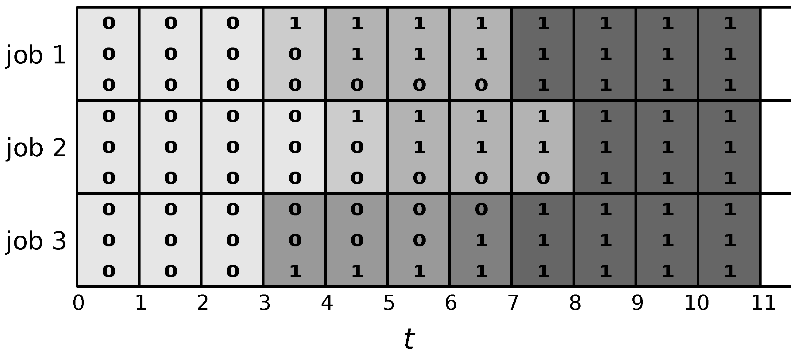
Figure 3.
A larger number of sets generated compared to those in Figure 2. Two of the original sets (indicated by bold borders) are split further into the dark grey and black sets.
Figure 3.
A larger number of sets generated compared to those in Figure 2. Two of the original sets (indicated by bold borders) are split further into the dark grey and black sets.

Figure 4.
This example considers the same toy instance, as in Figure 2, in which three jobs have to execute on three machines. The variable values (with respect to Model 1) are indicated for the same three solutions as those displayed in Figure 2.

Figure 5.
Comparison of the algorithms concerning the percentage difference to the best result, averaged over the instances with the same number of machines. The scale of the vertical axis is logarithmic.
Figure 5.
Comparison of the algorithms concerning the percentage difference to the best result, averaged over the instances with the same number of machines. The scale of the vertical axis is logarithmic.

Figure 6.
The performance of MS-ACO with 10, 15 and 20 cores. The results are averaged over instances with the same number of machines and show the gap to the best solution found by MS-ACO or CMSA-ACO.
Figure 6.
The performance of MS-ACO with 10, 15 and 20 cores. The results are averaged over instances with the same number of machines and show the gap to the best solution found by MS-ACO or CMSA-ACO.

Figure 7.
The performance of CMSA-ACO with 10, 15 and 20 cores. The results are averaged over instances with the same number of machines and show the gap to the best solution found by MS-ACO or CMSA-ACO.
Figure 7.
The performance of CMSA-ACO with 10, 15 and 20 cores. The results are averaged over instances with the same number of machines and show the gap to the best solution found by MS-ACO or CMSA-ACO.
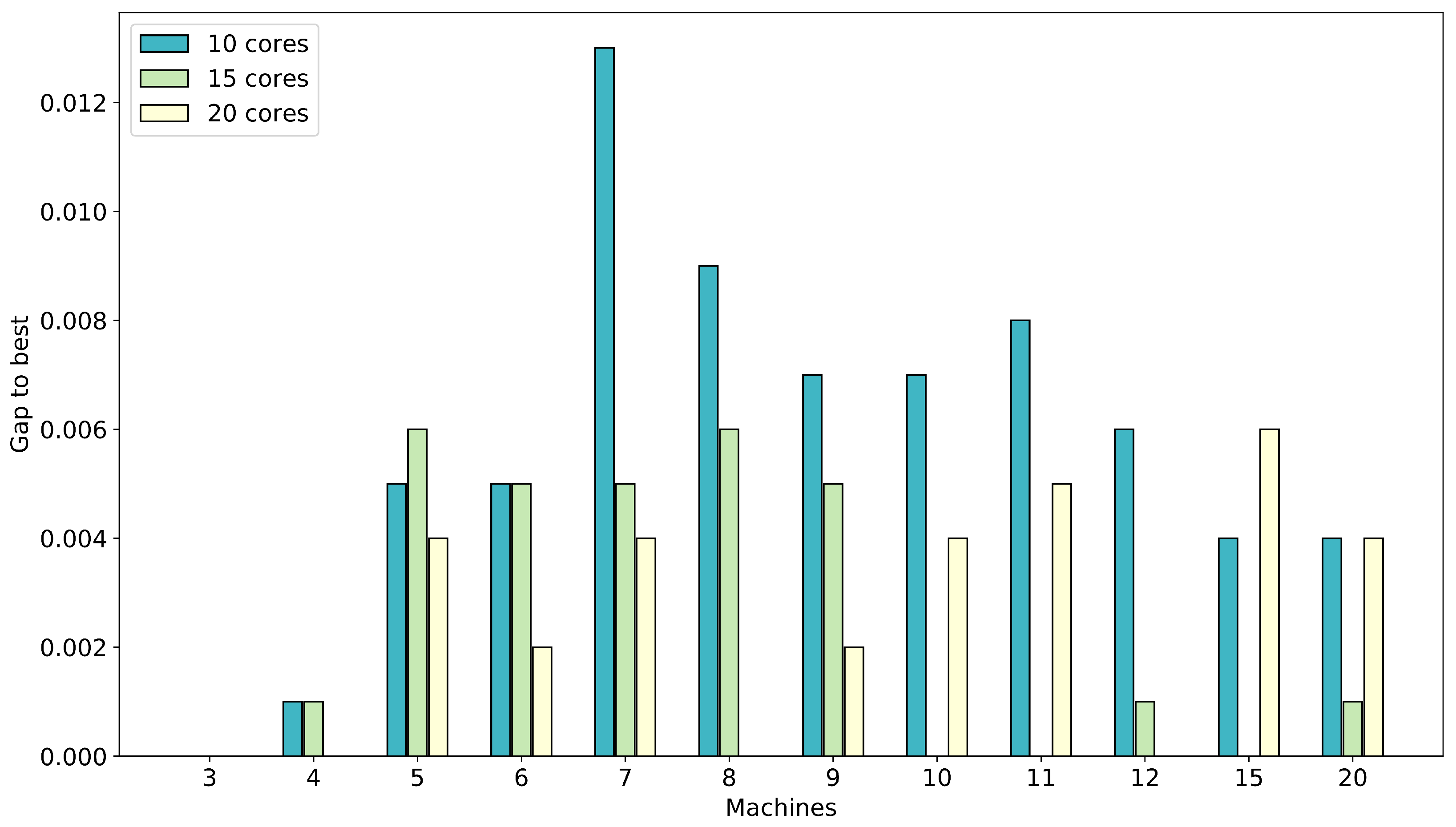
Figure 8.
Comparing the solution quality obtained by MS and CMSA when they are provided with the same set of solutions for one iteration. The boxes show the improvement in MS over CMSA (in percent), with a positive value indicating that CMSA performed better.
Figure 8.
Comparing the solution quality obtained by MS and CMSA when they are provided with the same set of solutions for one iteration. The boxes show the improvement in MS over CMSA (in percent), with a positive value indicating that CMSA performed better.
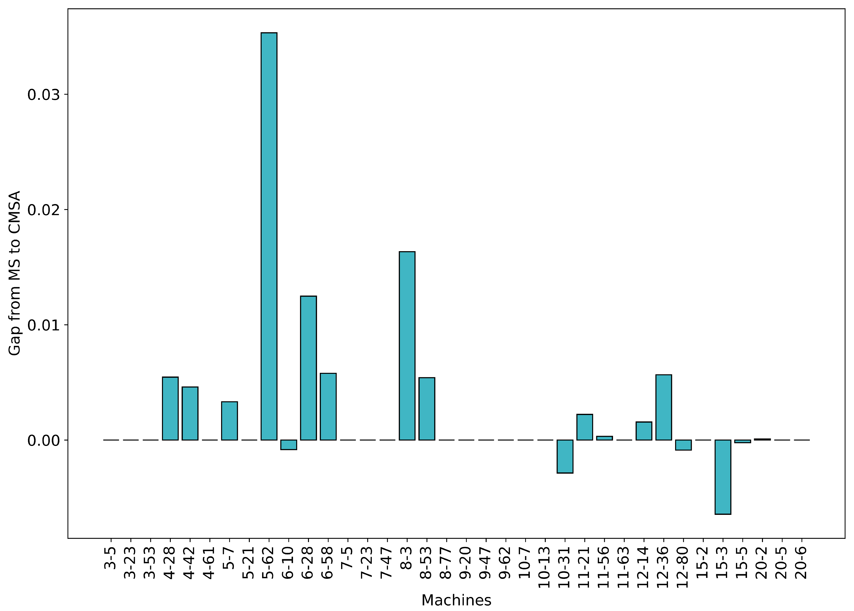
Figure 9.
Comparing the computing time needed by MS and CMSA for solving the restricted MIPs when they are provided with the same set of solutions for one iteration. The boxes show the percentage difference of MS and CMSA, with a positive value indicating that MS took more computation time.
Figure 9.
Comparing the computing time needed by MS and CMSA for solving the restricted MIPs when they are provided with the same set of solutions for one iteration. The boxes show the percentage difference of MS and CMSA, with a positive value indicating that MS took more computation time.

Table 1.
MS with ACO. For 25 runs conducted, the best () and average () solution qualities with associated standard deviations () are provided. The table also shows the average number of iterations () conducted for each problem instance. Statistically significant results, using a pairwise t-test, at the 95% confidence interval are highlighted in boldface.
| Inst. | MS-Heur | MS-ACO | ||||||
|---|---|---|---|---|---|---|---|---|
| Best | Mean | SD | Iter. | Best | Mean | SD | Iter. | |
| 3 -5 | 509.27 | 557.27 | 22.51 | 17,404.2 | 505.00 | 505.00 | 0.00 | 489.2 |
| 3 -23 | 151.83 | 161.71 | 5.03 | 20,000.6 | 149.07 | 149.07 | 0.00 | 619.5 |
| 3 -53 | 69.36 | 70.08 | 0.52 | 30,170.9 | 69.36 | 69.36 | 0.00 | 774.5 |
| 4 -28 | 25.62 | 28.57 | 1.41 | 17,529.3 | 23.81 | 23.81 | 0.00 | 398.7 |
| 4 -42 | 67.64 | 70.56 | 2.11 | 20,066.8 | 66.07 | 66.68 | 0.18 | 257.1 |
| 4 -61 | 45.96 | 49.18 | 2.24 | 16,211.5 | 45.96 | 45.96 | 0.00 | 362.2 |
| 5 -7 | 288.38 | 309.19 | 9.67 | 11,643.4 | 252.90 | 252.90 | 0.00 | 66.1 |
| 5 -21 | 168.63 | 177.50 | 3.57 | 10,962.0 | 168.63 | 168.63 | 0.00 | 293.6 |
| 5 -62 | 292.16 | 300.22 | 4.15 | 8095.0 | 249.50 | 255.42 | 3.21 | 20.2 |
| 6 -10 | 981.36 | 1031.48 | 21.78 | 2546.7 | 819.74 | 834.22 | 7.63 | 12.4 |
| 6 -28 | 261.38 | 290.74 | 9.51 | 10,087.2 | 218.37 | 218.37 | 0.00 | 39.4 |
| 6 -58 | 276.75 | 297.79 | 9.17 | 9739.5 | 236.05 | 237.87 | 1.30 | 17.7 |
| 7 -5 | 511.57 | 538.15 | 12.78 | 1549.9 | 419.52 | 430.83 | 6.42 | 28.5 |
| 7 -23 | 726.94 | 765.99 | 21.95 | 1006.2 | 540.40 | 561.70 | 8.46 | 27.0 |
| 7 -47 | 590.49 | 607.83 | 9.95 | 1224.2 | 412.60 | 438.96 | 10.86 | 27.0 |
| 8 -3 | 948.96 | 970.84 | 12.14 | 1376.2 | 615.93 | 648.25 | 15.46 | 23.8 |
| 8 -53 | 558.03 | 579.63 | 11.40 | 413.0 | 447.37 | 465.85 | 8.36 | 26.0 |
| 8 -77 | 1469.22 | 1548.06 | 29.05 | 1667.9 | 1186.69 | 1216.34 | 14.35 | 25.0 |
| 9 -20 | 1095.74 | 1135.18 | 18.01 | 25.2 | 905.02 | 926.73 | 11.41 | 24.0 |
| 9 -47 | 1579.50 | 1626.32 | 29.89 | 133.3 | 1200.87 | 1226.92 | 14.59 | 20.9 |
| 9 -62 | 1775.97 | 1819.71 | 24.57 | 371.2 | 1422.05 | 1449.17 | 12.95 | 22.0 |
| 10 -7 | 3187.99 | 3297.69 | 54.14 | 51.2 | 2522.62 | 2581.62 | 31.52 | 20.0 |
| 10 -13 | 2736.23 | 2839.93 | 44.65 | 29.9 | 2156.04 | 2217.89 | 29.63 | 20.0 |
| 10 -31 | 764.95 | 816.82 | 16.02 | 303.9 | 591.21 | 618.68 | 11.10 | 22.0 |
| 11 -21 | 1194.71 | 1246.61 | 22.19 | 57.1 | 997.39 | 1023.32 | 18.41 | 21.0 |
| 11 -56 | 2230.69 | 2321.07 | 34.10 | 329.5 | 1800.44 | 1851.90 | 26.64 | 18.0 |
| 11 -63 | 2386.59 | 2445.65 | 23.56 | 31.5 | 2003.32 | 2034.60 | 12.50 | 19.0 |
| 12 -14 | 2241.26 | 2335.04 | 34.55 | 46.4 | 1750.58 | 1803.95 | 18.14 | 18.0 |
| 12 -36 | 4021.57 | 4147.06 | 43.38 | 27.6 | 2991.41 | 3047.97 | 38.77 | 16.0 |
| 12 -80 | 3093.55 | 3197.13 | 43.97 | 21.1 | 2399.97 | 2430.03 | 16.96 | 16.4 |
| 15 -2 | 5372.02 | 5494.10 | 60.88 | 55.7 | 4003.67 | 4110.89 | 47.28 | 10.0 |
| 15 -3 | 6215.61 | 6360.31 | 68.50 | 51.7 | 4483.49 | 4558.71 | 32.51 | 11.3 |
| 15 -5 | 5311.44 | 5493.00 | 85.55 | 23.1 | 3541.96 | 3576.02 | 20.02 | 13.0 |
| 20 -2 | 9994.59 | 10,370.08 | 124.46 | 24.3 | 8831.20 | 8961.45 | 47.51 | 6.0 |
| 20 -5 | 17,213.70 | 18,168.91 | 578.03 | 38.8 | 14,708.02 | 14,951.71 | 102.72 | 5.0 |
| 20 -6 | 9616.81 | 9748.11 | 67.32 | 30.0 | 7890.31 | 8081.78 | 68.45 | 7.1 |
Table 2.
CMSA with ACO. For 25 runs conducted, the best () and average () solution qualities with associated standard deviations () are provided. The table also shows the average number of iterations () conducted for each problem instance. Statistically significant results, using a pairwise t-test, at the 95% confidence interval are highlighted in boldface.
| Inst. | CMSA-Heur | CMSA-ACO | ||||||
|---|---|---|---|---|---|---|---|---|
| Best | Mean | SD | Iter. | Best | Mean | SD | Iter. | |
| 3 -5 | 594.31 | 610.85 | 13.03 | 110.0 | 505.00 | 505.00 | 0.00 | 324.2 |
| 3 -23 | 174.23 | 179.03 | 2.52 | 198.8 | 149.07 | 149.07 | 0.00 | 476.0 |
| 3 -53 | 69.36 | 69.36 | 0.00 | 624.1 | 69.36 | 69.36 | 0.00 | 755.5 |
| 4 -28 | 25.37 | 26.62 | 0.85 | 215.6 | 23.81 | 23.81 | 0.00 | 346.3 |
| 4 -42 | 88.12 | 96.82 | 3.49 | 67.9 | 66.07 | 66.26 | 0.25 | 27.3 |
| 4 -61 | 45.96 | 46.07 | 0.04 | 266.6 | 45.96 | 45.96 | 0.00 | 298.0 |
| 5 -7 | 396.81 | 423.44 | 14.83 | 33.1 | 252.90 | 252.90 | 0.00 | 19.1 |
| 5 -21 | 168.63 | 238.71 | 26.81 | 34.0 | 168.63 | 168.63 | 0.00 | 129.6 |
| 5 -62 | 273.95 | 290.95 | 15.57 | 33.2 | 249.50 | 254.42 | 3.69 | 13.0 |
| 6 -10 | 834.65 | 1086.32 | 93.43 | 33.0 | 825.64 | 837.68 | 5.71 | 12.4 |
| 6 -28 | 298.54 | 346.66 | 30.39 | 33.8 | 218.37 | 218.40 | 0.05 | 13.2 |
| 6 -58 | 350.63 | 391.62 | 25.49 | 33.7 | 236.05 | 238.50 | 1.11 | 13.0 |
| 7 -5 | 430.28 | 493.74 | 34.04 | 30.7 | 420.20 | 433.92 | 5.41 | 28.4 |
| 7 -23 | 704.54 | 760.36 | 26.65 | 33.1 | 553.02 | 562.97 | 6.39 | 27.0 |
| 7 -47 | 493.25 | 585.79 | 51.19 | 32.6 | 419.60 | 441.67 | 11.99 | 26.9 |
| 8 -3 | 1176.16 | 1350.22 | 148.12 | 33.0 | 621.74 | 658.87 | 15.50 | 23.9 |
| 8 -53 | 459.59 | 537.54 | 42.67 | 33.3 | 442.83 | 457.30 | 8.06 | 26.0 |
| 8 -77 | 2017.81 | 2144.72 | 81.62 | 33.1 | 1183.94 | 1211.27 | 13.94 | 25.0 |
| 9 -20 | 1068.60 | 1149.51 | 36.80 | 33.0 | 903.30 | 928.40 | 10.04 | 24.0 |
| 9 -47 | 1974.63 | 2200.42 | 146.16 | 33.0 | 1205.99 | 1226.62 | 11.03 | 20.4 |
| 9 -62 | 2055.12 | 2214.52 | 115.67 | 32.9 | 1410.96 | 1449.41 | 15.43 | 22.0 |
| 10 -7 | 3268.61 | 3551.05 | 143.94 | 33.1 | 2491.08 | 2557.32 | 33.20 | 20.0 |
| 10 -13 | 3380.87 | 3834.01 | 265.64 | 31.5 | 2149.49 | 2205.24 | 30.19 | 20.0 |
| 10 -31 | 730.47 | 838.64 | 46.29 | 33.0 | 592.08 | 610.79 | 8.33 | 22.3 |
| 11 -21 | 1298.52 | 1332.68 | 33.66 | 30.0 | 997.08 | 1011.50 | 8.38 | 21.0 |
| 11 -56 | 2832.30 | 2989.67 | 138.04 | 33.0 | 1793.48 | 1834.68 | 18.19 | 18.0 |
| 11 -63 | 2521.33 | 2723.58 | 137.40 | 33.0 | 1988.45 | 2025.39 | 18.71 | 19.0 |
| 12 -14 | 2154.49 | 2437.09 | 170.98 | 32.9 | 1737.87 | 1788.23 | 16.39 | 18.0 |
| 12 -36 | 4600.80 | 4832.21 | 111.99 | 33.0 | 2917.00 | 2989.84 | 38.90 | 16.1 |
| 12 -80 | 3336.94 | 3490.43 | 79.00 | 31.2 | 2363.39 | 2411.98 | 17.79 | 17.0 |
| 15 -2 | 5611.15 | 5851.75 | 116.12 | 32.2 | 3967.47 | 4041.84 | 38.95 | 10.0 |
| 15 -3 | 7484.49 | 7666.97 | 113.31 | 32.4 | 4352.50 | 4476.71 | 60.64 | 11.0 |
| 15 -5 | 4832.37 | 5311.91 | 202.94 | 33.0 | 3397.36 | 3520.99 | 40.72 | 13.0 |
| 20 -2 | 11,438.07 | 11,550.36 | 71.87 | 29.0 | 8733.86 | 8913.17 | 96.27 | 6.0 |
| 20 -5 | 20,478.46 | 20,891.89 | 237.81 | 30.4 | 14,588.81 | 14,894.91 | 159.12 | 5.0 |
| 20 -6 | 9791.88 | 9941.69 | 84.49 | 32.0 | 7800.87 | 7968.64 | 79.34 | 7.0 |
Table 3.
A comparison of CGACO, CGDELS and BRKGA against MS and CMSA. The results are presented as the % difference from each method to the best known solution (column 2). The time limits for solving the restricted MIPs within MS-ACO and CMSA-ACO were set to 120 s. The best results are in bold. Statistically significant results, using a pairwise t-test, at the 95% confidence interval are italicized.
| Inst. | Best | CGACO | CGDELS | BRKGA | MS-ACO | CMSA-ACO |
|---|---|---|---|---|---|---|
| 3 -5 | 505.0 | 0.1083 | 0.0000 | 0.0000 | 0.0000 | 0.0000 |
| 3 -23 | 149.1 | 0.0923 | 0.0012 | 0.0000 | 0.0000 | 0.0000 |
| 3 -53 | 69.4 | 0.0095 | 0.0027 | 0.0000 | 0.0000 | 0.0000 |
| 4 -28 | 23.8 | 0.2066 | 0.0038 | 0.0050 | 0.0000 | 0.0000 |
| 4 -42 | 66.1 | 0.0652 | 0.0148 | 0.0238 | 0.0092 | 0.0029 |
| 4 -61 | 46.0 | 0.0570 | 0.0000 | 0.0111 | 0.0000 | 0.0000 |
| 5 -7 | 252.9 | 0.2192 | 0.0022 | 0.0031 | 0.0000 | 0.0000 |
| 5 -21 | 168.6 | 0.0503 | 0.0000 | 0.0000 | 0.0000 | 0.0000 |
| 5 -62 | 249.5 | 0.2052 | 0.0197 | 0.0247 | 0.0237 | 0.0197 |
| 6 -10 | 811.6 | 0.2709 | 0.0162 | 0.0203 | 0.0278 | 0.0321 |
| 6 -28 | 218.4 | 0.3493 | 0.0068 | 0.0444 | 0.0000 | 0.0001 |
| 6 -58 | 236.1 | 0.2747 | 0.0255 | 0.0224 | 0.0077 | 0.0104 |
| 7 -5 | 418.1 | 0.2849 | 0.0220 | 0.0289 | 0.0305 | 0.0379 |
| 7 -23 | 533.8 | 0.4319 | 0.0382 | 0.0446 | 0.0524 | 0.0547 |
| 7 -47 | 406.4 | 0.5121 | 0.0345 | 0.0298 | 0.0803 | 0.0869 |
| 8 -3 | 615.9 | 0.5709 | 0.0305 | 0.0225 | 0.0525 | 0.0697 |
| 8 -53 | 442.2 | 0.3025 | 0.0318 | 0.0241 | 0.0535 | 0.0342 |
| 8 -77 | 1163.8 | 0.3272 | 0.0419 | 0.0262 | 0.0452 | 0.0408 |
| 9 -20 | 873.3 | 0.2936 | 0.0157 | 0.0102 | 0.0612 | 0.0631 |
| 9 -47 | 1158.3 | 0.4145 | 0.0570 | 0.0236 | 0.0593 | 0.0590 |
| 9 -62 | 1382.6 | 0.3072 | 0.0512 | 0.0123 | 0.0481 | 0.0483 |
| 10 -7 | 2384.0 | 0.3862 | 0.0341 | 0.0068 | 0.0829 | 0.0727 |
| 10 -13 | 2082.7 | 0.3612 | 0.0298 | 0.0116 | 0.0649 | 0.0588 |
| 10 -31 | 572.0 | 0.4260 | 0.0421 | 0.0258 | 0.0816 | 0.0678 |
| 11 -21 | 964.0 | 0.2939 | 0.0315 | 0.0098 | 0.0615 | 0.0492 |
| 11 -56 | 1674.5 | 0.3961 | 0.0698 | 0.0121 | 0.1059 | 0.0957 |
| 11 -63 | 1887.2 | 0.2990 | 0.0544 | 0.0136 | 0.0781 | 0.0732 |
| 12 -14 | 1636.4 | 0.4313 | 0.0517 | 0.0132 | 0.1024 | 0.0928 |
| 12 -36 | 2764.2 | 0.4965 | 0.0432 | 0.0119 | 0.1027 | 0.0816 |
| 12 -80 | 2226.7 | 0.4439 | 0.0532 | 0.0141 | 0.0913 | 0.0832 |
| 15 -2 | 3596.5 | 0.5376 | 0.0663 | 0.0086 | 0.1430 | 0.1238 |
| 15 -3 | 3948.2 | 0.6075 | 0.0715 | 0.0117 | 0.1546 | 0.1339 |
| 15 -5 | 3234.7 | 0.6981 | 0.0613 | 0.0124 | 0.1055 | 0.0885 |
| 20 -2 | 7755.3 | 0.3437 | 0.0712 | 0.0174 | 0.1555 | 0.1493 |
| 20 -5 | 12,899.2 | 0.4139 | 0.0857 | 0.0174 | 0.1591 | 0.1547 |
| 20 -6 | 6907.8 | 0.4101 | 0.0634 | 0.0131 | 0.1699 | 0.1536 |
Table 4.
The contribution of the merge step of MS-ACO and CMSA-ACO, relative to the total solution improvement. The MIP results sum up the percentage improvement in the objective for every MIP solve for an instance. The MS/CMSA+ACO result is the percentage difference of the first best solution found to the best solution at the end of the run. Small instances where the best solution is the first one found have been omitted.
| Inst. | MS-MIP | MS + ACO | CMSA-MIP | CMSA + ACO |
|---|---|---|---|---|
| 4 - 28 | 1.72 | 3.13 | 1.69 | 2.37 |
| 4 - 42 | 0.86 | 1.87 | 2.25 | 3.31 |
| 5 - 7 | 7.30 | 8.23 | 7.94 | 8.63 |
| 5 - 62 | 3.14 | 6.00 | 3.46 | 4.66 |
| 6 - 10 | 1.36 | 2.38 | 0.25 | 1.86 |
| 6 - 28 | 2.81 | 2.96 | 2.46 | 2.55 |
| 6 - 58 | 2.58 | 3.09 | 2.77 | 3.14 |
| 7 - 5 | 3.47 | 5.56 | 2.56 | 4.23 |
| 7 - 23 | 2.02 | 5.41 | 1.60 | 6.48 |
| 7 - 47 | 3.63 | 7.70 | 1.40 | 7.52 |
| 8 - 3 | 4.98 | 8.29 | 2.65 | 5.57 |
| 8 - 53 | 1.30 | 1.95 | 1.41 | 4.82 |
| 8 - 77 | 0.93 | 3.52 | 1.03 | 4.73 |
| 9 - 20 | 2.20 | 4.43 | 1.24 | 3.61 |
| 9 - 47 | 1.47 | 3.26 | 0.93 | 3.33 |
| 9 - 62 | 1.06 | 2.79 | 0.49 | 2.25 |
| 10 - 7 | 1.09 | 2.29 | 0.96 | 3.37 |
| 10 - 13 | 0.87 | 2.69 | 0.36 | 2.48 |
| 10 - 31 | 1.70 | 3.96 | 1.19 | 4.65 |
| 11 - 21 | 1.17 | 2.89 | 0.91 | 3.96 |
| 11 - 56 | 0.69 | 2.38 | 0.58 | 3.96 |
| 11 - 63 | 0.47 | 2.69 | 0.42 | 2.09 |
| 12 - 14 | 0.88 | 3.16 | 1.35 | 3.82 |
| 12 - 36 | 0.49 | 2.14 | 1.19 | 3.85 |
| 12 - 80 | 0.36 | 2.80 | 0.95 | 3.27 |
| 15 - 2 | 0.49 | 2.28 | 0.36 | 2.68 |
| 15 - 3 | 0.46 | 1.47 | 0.29 | 3.39 |
| 15 - 5 | 0.63 | 1.49 | 0.98 | 3.81 |
| 20 - 2 | 0.09 | 1.07 | 0.06 | 1.77 |
| 20 - 5 | 0.13 | 0.67 | 0.04 | 1.60 |
| 20 - 6 | 0.12 | 0.45 | 0.06 | 1.96 |
© 2020 by the authors. Licensee MDPI, Basel, Switzerland. This article is an open access article distributed under the terms and conditions of the Creative Commons Attribution (CC BY) license (http://creativecommons.org/licenses/by/4.0/).
Share and Cite
MDPI and ACS Style
Thiruvady, D.; Blum, C.; Ernst, A.T. Solution Merging in Matheuristics for Resource Constrained Job Scheduling. Algorithms 2020, 13, 256. https://0-doi-org.brum.beds.ac.uk/10.3390/a13100256
AMA Style
Thiruvady D, Blum C, Ernst AT. Solution Merging in Matheuristics for Resource Constrained Job Scheduling. Algorithms. 2020; 13(10):256. https://0-doi-org.brum.beds.ac.uk/10.3390/a13100256
Chicago/Turabian StyleThiruvady, Dhananjay, Christian Blum, and Andreas T. Ernst. 2020. "Solution Merging in Matheuristics for Resource Constrained Job Scheduling" Algorithms 13, no. 10: 256. https://0-doi-org.brum.beds.ac.uk/10.3390/a13100256
Note that from the first issue of 2016, this journal uses article numbers instead of page numbers. See further details here.