Blind Quality Evaluation for Screen Content Images Based on Regionalized Structural Features

Abstract

Currently, screen content images (SCIs) are widely used in our modern society. However, since SCIs have distinctly different properties compared to natural images, traditional quality assessment methods of natural images cannot precisely evaluate the quality of SCIs. Thus, we propose a blind quality evaluation method for SCIs based on regionalized structural features that are closely relevant to the intrinsic quality of SCIs. Firstly, the features of textual and pictorial regions of SCIs are extracted separately. For textual regions, since they contain noticeable structural information, we propose improved histograms of oriented gradients extracted from multi-order derivatives as structural features. For pictorial regions, since human vision is sensitive to texture information and luminance variation, we adopt texture as the structural feature; meanwhile, luminance is used as the auxiliary feature. The local derivative pattern and the shearlet local binary pattern are used to extract texture in the spatial and shearlet domains, respectively. Secondly, to derive the quality of textual and pictorial regions, two mapping functions are respectively trained from their features to subjective values. Finally, an activity weighting strategy is proposed to combine the quality of textual and pictorial regions. Experimental results show that the proposed method achieves better performance than the state-of-the-art methods.

1. Introduction

Recently, screen content images (SCIs) have been widely applied as a form of information representation in our modern society owing to the popularization of multimedia applications including remote screen sharing, Cloud and mobile computing, commodity advertisements of online shopping websites and real-time online teaching [1,2]. In many actual engineering applications, including compression, storage, transmission and display, the visual quality of SCIs will inevitably be degraded owing to distortions including noise, blur, contrast variation, blockiness and quantization loss. Undoubtedly, the quality degradation of SCIs will significantly affect the visual perception of observers. Thus, it is necessary and meaningful to develop quality evaluation methods for SCIs in actual engineering applications.

Over recent decades, a large number of image quality assessment (IQA) methods have been elaborately designed and applied in the field of digital image processing. The peak signal-to-noise ratio (PSNR) is a conventional IQA method and has been applied extensively. However, it has inferior prediction performance since it only deals with the difference between pixels and does not take into account the perceptual properties of human vision. To overcome this drawback, the research community has proposed many advanced full-reference (FR) IQA metrics that require the entire information of the reference image. These metrics skillfully model intrinsic properties of the human visual system (HVS) and representative metrics include structure similarity (SSIM) [3], feature similarity [4], visual information fidelity [5], gradient magnitude similarity deviation (GMSD) [6], the internal generative mechanism (IGM) metric [7] and deep similarity [8]. In [3], the quality of an image is measured by combining the changes from the luminance, contrast and structure. In [4], two complementary low-level features, namely the phase congruency and the image gradient magnitude, are adopted to characterize the image local quality. In [5], the loss of image information is quantified and used to assess the visual quality of an image. In [6], the standard deviation of the gradient magnitude similarity map is calculated as the quality index of an image. In [7], according to the IGM theory, an autoregressive prediction method is used to decompose an image into the predicted and disorderly parts whose distortions are measured by the structural similarity and the PSNR, respectively. In [8], the local similarities of features generated by the convolutional neural network (CNN) are calculated and pooled together to assess the quality of an image.

Additionally, alongside the FR IQA metrics, some reduced-reference (RR) IQA metrics [9], and no-reference/blind IQA metrics [10], have also been presented over recent decades. The RR IQA metrics only need partial information of the reference image, while the no-reference (NR) IQA metrics need no information from the reference image. Many blind IQA methods first extract quality-aware features and then these features are supplied into a machine learning model to obtain the quality assessment result. Mittal et al. [11], presented a blind IQA metric called BRISQUE in which the naturalness of an image is quantified and natural scene statistics (NSS) features of locally normalized luminance values are adopted. Li et al. [12], presented a blind IQA metric which adopts two types of features, namely the luminance features represented by the luminance histogram and the structural features denoted by the histogram of the local binary pattern (LBP) of the normalized luminance. Li et al. [13], designed a blind IQA metric based on structural features denoted by the gradient-weighted histogram of the LBP computed from gradient values. In [14,15], the statistical histograms of the texture information of an image are extracted as quality-aware features to describe the distortion degree of the image. In [16], NSS features extracted from reference images are used to learn a multivariate Gaussian model and then this learned model is used to evaluate the quality of distorted images.

Although the IQA methods mentioned above obtain superior performance, they have been specially developed to predict the quality of natural images and cannot be used to precisely assess the quality of SCIs. The reason for this is that SCIs have some distinctly different characteristics compared to natural images. Firstly, their contents are different. Generally, texts, natural images, slides and logos are mixed in an SCI and so an SCI has rough edges, simple shapes, thin lines and a small number of colors. Two typical examples of SCIs are shown in Figure 1. However, a natural image contains continuous-tone content with slow-varying edges, complicated structures, thick lines and more colors. Secondly, their statistical distributions are different. In general, after luminance values of a natural image are processed by the mean subtracted contrast normalized (MSCN) operation, their statistical distribution can be modeled by a Gaussian function [11]. By comparison, for an SCI, this statistical distribution behaves like a Laplacian contour [17] and the curve of this statistical distribution varies dramatically. Specifically, the center of this curve has a keen-edged pimpling and the remaining parts are still wavy [18]. Thirdly, their image activity levels [19], are different. Because the pixel values of an SCI have greater variations in local regions, the activity measurement value of an SCI is greater than that of a natural image [18]. As SCIs and natural images have these different properties, users have completely different viewing experiences regarding the quality degradation of SCIs and natural images. Therefore, the existing IQA methods developed for natural images are inappropriate to assess the quality of SCIs.

To date, a few algorithms have been proposed to perform the quality evaluation of SCIs. The earliest study of the quality assessment of SCIs was conducted by Yang et al. [18], who proposed an FR screen content image quality assessment (SCIQA) method called SPQA. In this method, for textual layers of SCIs, both luminance and sharpness similarities are calculated, while for pictorial layers of SCIs, only the sharpness similarity is computed. Respective quality values of textual and pictorial layers are combined as the overall quality score of a distorted SCI by employing a weighting activity map. However, the predictive performance of the SPQA method needs to be improved further. Fang et al. [20], proposed an FR SCIQA method, in which the similarity of structural features denoted by the gradient information is calculated to estimate the quality of textual regions of the SCI and the similarities of luminance features and structural features denoted by the LBP features are computed to predict the quality of pictorial regions of the SCI. Ni et al. [21], explored the edge variation of SCIs in depth and employed three edge characteristics including the contrast, width and direction of edges, which are extracted from a parametric edge model. Fu et al. [22], adopted a two-scale difference-of-Gaussian (DOG) filter to extract the edges of an SCI and the similarities of small-scale edges are calculated and combined by using larger-scale edges as weighting values. Wang et al. [23], designed an FR SCIQA method based on edge characteristics extracted from gradient values, which include the edge sharpness, the edge brightness change, the edge contrast change and the edge chrominance. In [24], the local similarities of two chrominance components and Gabor features generated by the imaginary part of the Gabor filer are computed and combined to produce the assessment score. In [25], statistical features of the primary visual and uncertainty information are used to design an RR SCIQA metric. Wang et al. [26], proposed an RR quality assessment method of compressed SCIs in which wavelet domain features including the mean, variance and entropy of wavelet coefficients are used to learn a regression model. Rahul et al. [27], presented an RR SCIQA method based on feature points identified by the cascade DOG filters. The aforementioned methods of SCIs [21,22,23,24,25,26,27] have one common drawback: they employ the same feature representation method to characterize the quality degradation of the entire content of SCIs and do not take different steps to deal with the different contents of SCIs. Since human eyes have an obviously different visual experience to the distortions of the textual and pictorial contents contained in SCIs, it is unreasonable to employ the same features to denote the quality degradation of the textual and pictorial content of SCIs. Additionally, these FR or RR methods require the entire or partial information of reference SCIs which cannot be acquired in the majority of actual cases.

Gu et al. [28], put forward an NR SCIQA model in which one free energy feature and twelve structural degradation features are extracted to train the assessment model. Yue et al. [29], designed a blind SCIQA method based on the CNN, in which both the predicted and unpredicted parts obtained according to the IGM theory are inputted into the CNN. However, in [28,29], predictive values generated by objective FR SCIQA methods rather than subjective ratings values are used as training labels, which may result in a deviation. In [30], local and global sparse representations are conducted to design an NR SCIQA model. Lu et al. [31], performed the blind quality assessment of SCIs based on statistical orientation features and structural features denoted by the LBP histograms of nine gradient maps. Min et al. [32], proposed an NR quality evaluation method of compressed SCIs in which the features of corners and edges at multiple scales are integrated by using a multi-scale weighting strategy. Fang et al. [33], presented a blind SCIQA model by considering both local features denoted by the histograms of locally normalized luminance values and global features denoted by the histograms of the texture features extracted from gradient maps. Gu et al. [17], developed a blind assessment model of SCIs comprising four elements, namely picture complexity, screen content statistics, brightness and sharpness. Although these existing blind evaluation models, which were specifically developed for SCIs, obtain better prediction performance compared to traditional evaluation models of natural images, they still cannot obtain a high prediction accuracy and there is still a great deal of room to enhance their performances. Thus, the blind quality assessment of SCIs remains a challenging problem and needs to be further investigated in depth by the research community.

To further improve the predictive accuracy of existing blind evaluation methods of SCIs, in this study, we propose a blind SCIQA method based on regionalized structural features (BSRSF) which are closely relevant to the intrinsic quality of SCIs. Firstly, considering very different characteristics of the textual and pictorial content in an SCI, the SCI is segmented into two completely different types: textual regions and pictorial regions. Secondly, to derive respective assessment values of textual and pictorial regions, their features are respectively extracted by applying different methods according to their characteristics and then they are separately supplied to machine learning models, i.e., support vector regression (SVR). Specifically, given the noticeable structural information contained in textual regions, the structural information is used as the quality-aware feature of textual regions. For pictorial regions, since human vision is sensitive to texture information and luminance variation, texture features are used as structural features; meanwhile, the luminance information is used as the auxiliary feature. Finally, an activity weighting strategy is proposed to fuse the assessment values of textual and pictorial regions as the final assessment value of this degraded SCI. Experimental results show that the proposed BSRSF method achieves better prediction performance than other existing blind SCIQA methods on SIQAD and SCID, which are often employed as validation databases of SCIs. In contrast to the existing blind SCIQA methods, the main contributions of the proposed BSRSF metric are as follows:

(1)

We propose improved histograms of the oriented gradients, which are extracted from the multi-order derivatives. In the proposed method, these histograms are adopted as structural features to predict the quality of textual regions of SCIs.

(2)

We extract texture features from both the spatial and shearlet domains as structural features of pictorial regions. The statistical histograms of the local derivative pattern are used as texture features in the spatial domain. We propose a new local pattern descriptor called the shearlet local binary pattern to represent texture features in the shearlet domain. To the best of our knowledge, this is the first attempt to extract texture features from the shearlet domain.

(3)

We propose an activity weighting strategy to combine the visual quality of textual and pictorial regions. This strategy is based on the activity degree of different regions in the SCI, in which the weights are extracted from gradient values of this SCI.

The remaining content of this paper is organized as follows. The detailed content of the proposed BSRSF method is presented stage-by-stage in Section 2. Experimental results are given in Section 3. Finally, the conclusions of this paper are presented in Section 4.

2. Proposed Method

In this section, the proposed BSRSF method is described in detail. The framework of the BSRSF method is illustrated in Figure 2, which includes two parts: the training process and the evaluation process. For the training process, the training SCIs are divided into textual and pictorial regions and then their features are individually extracted and fed into respective learning tools, namely the SVR. Meanwhile, subjective ratings values of the training SCIs are also fed into the SVR to train the corresponding regression models. For the evaluation process, we first employ the same partition and feature extraction methods and the features extracted from textual and pictorial regions of a distorted SCI are directly fed into corresponding regression models. Then, we can derive respective assessment scores of textual and pictorial regions. Finally, assessment scores of textual and pictorial regions are incorporated together as the final objective assessment score of this distorted SCI.

2.1. SCI Partition

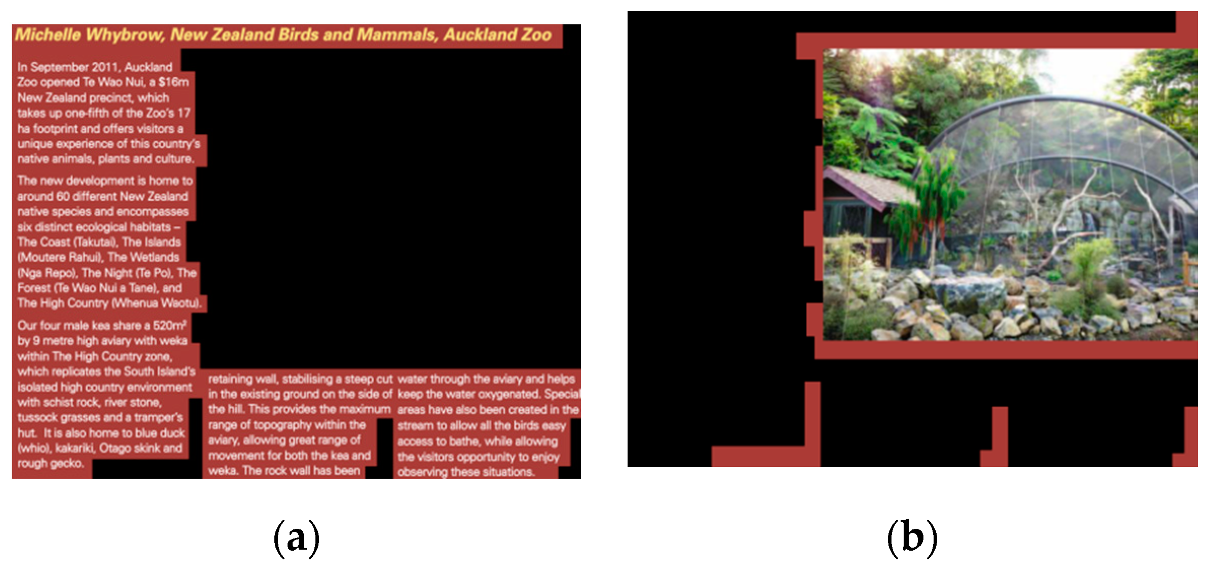
Up to now, the research community has put forward a number of image segmentation methods, such as superpixel segmentation methods [34,35], watershed-based segmentation methods [36,37], and active contour models [38,39]. In this paper, a text segmentation method in [19], is used to divide an SCI into two completely different types: textual regions and pictorial regions. In this method, a coarse-to-fine strategy is used to segment the textual content from an inputted SCI. Firstly, a local image activity measure algorithm is used to partition an SCI into pictorial regions and coarse texture regions, which include the textual content and a small amount of the pictorial content with high activity. Next, to remove fake text in coarse textual regions, the refinement procedure based on textual connected components is further applied to coarse texture regions. An example of this segmentation method is shown in Figure 3.

2.2. Feature Extraction of Textual Regions

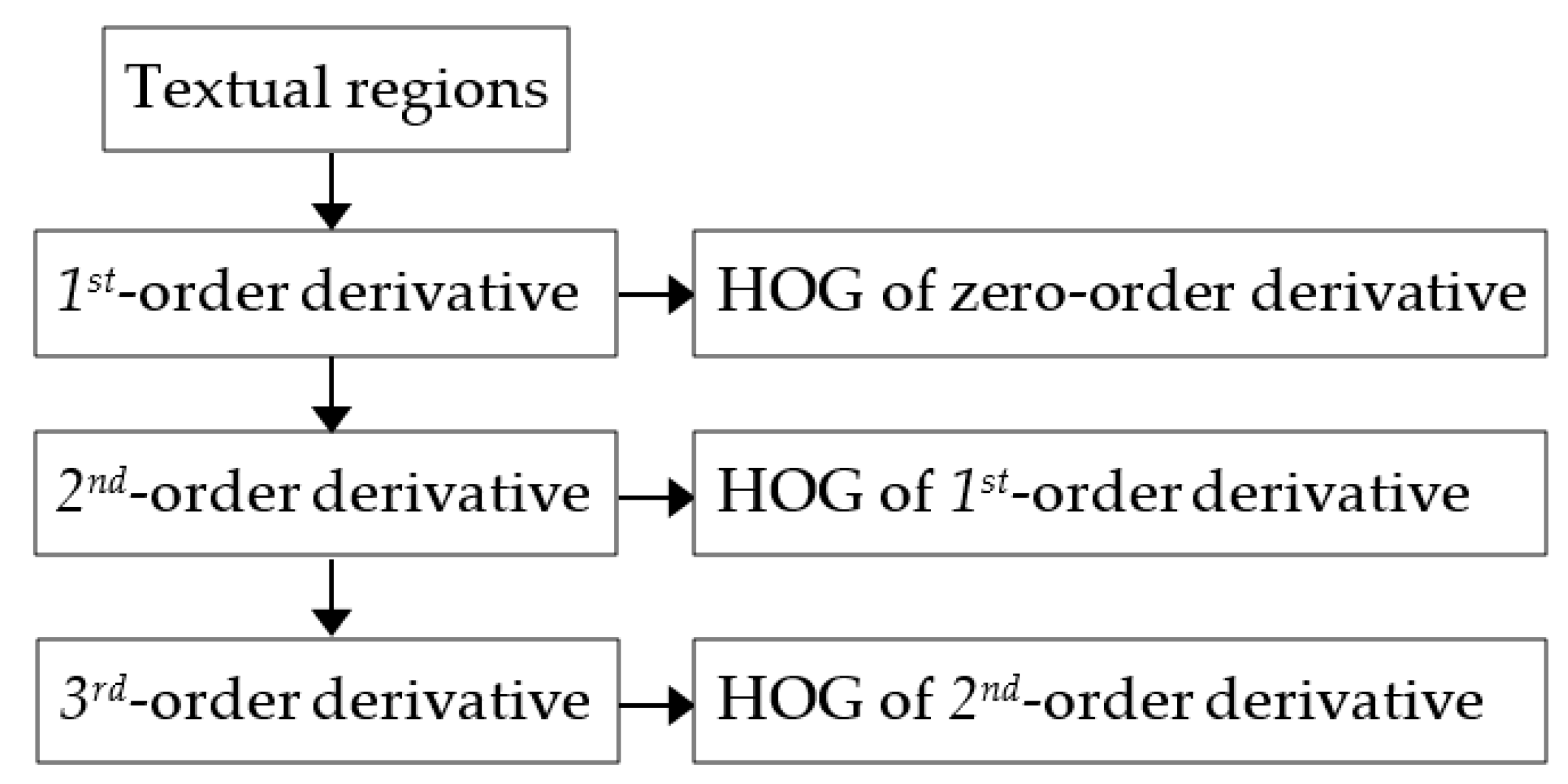
In the proposed BSRSF metric, structural features of textual regions of an SCI are extracted from the values of multi-order derivatives. The framework of the feature extraction of textual regions is depicted in Figure 4.

It is well known that a mass of characters exists in textual regions of SCIs and characters have diverse edges. Thus, textual regions of SCIs possess noticeable structural characteristics. The existing literature indicates that the multi-order derivatives can accurately describe the structural characteristics and the derivative information of different orders is closely correlated with different structural characteristics [40,41]. The first-order derivative information is correlated with the slope and elasticity of a landscape, the second-order derivative information can represent the curvature of a landscape [40], and the higher-order derivative information can provide tiny distinguishing structural details of a landscape [41]. Thus, the derivative information of different orders can efficiently denote the structural changes of an image, which have an important effect on the perceptual distortion of SCIs. Further, since derivative values of different orders have different characteristics, they should be combined to supply more comprehensive structural information for IQA methods.

To accurately depict the local structure of textual regions in SCIs, the magnitude and orientation of multi-order derivatives should be incorporated together. Therefore, in this paper, an improved histogram of oriented gradient (IHOG) descriptor is proposed to extract statistical features of the magnitude and orientation of multi-order derivatives. The histogram of oriented gradient (HOG) descriptor considers the statistical distribution of the gradient directions in a small patch of an image; meanwhile, the gradient magnitudes in this small patch are also incorporated into the HOG. The HOG descriptor was initially proposed to deal with the problem of human detection [42]. The underlying notion of the HOG descriptor is that the feature of the object shape in a small patch can be depicted accurately by the statistical distribution of the gradient values of this patch and the actual gradient values of this patch do not need to be known. Specifically, for the IHOG descriptor, the original gray values of textual regions are viewed as the zero-order derivative of textual regions and then the HOG descriptor of the zero-order derivative is calculated by employing the magnitude and orientation of the first-order derivative; the HOG descriptor of the first-order derivative is derived based on the magnitude and orientation of the second-order derivative; and similarly, the HOG descriptor of the nth-order derivative is calculated based on the magnitude and orientation of the (n + 1)th-order derivative.

Firstly, in this paper, the Prewitt filter is adopted to calculate the multi-order derivatives since its computation is simple. The first-order derivative of textual regions of an SCI is calculated as

$$d_h^1\left(x,y\right)=S_T\left(x,y\right)\ast P_h,P_h=\frac{1}{3}\left[\begin{array}{ccc}-1& 0& 1\\ -1& 0& 1\\ -1& 0& 1\end{array}\right]$$

(1)

$$d_v^1\left(x,y\right)=S_T\left(x,y\right)\ast P_v,P_v=\frac{1}{3}\left[\begin{array}{ccc}-1& -1& -1\\ 0& 0& 0\\ 1& 1& 1\end{array}\right]$$

(2)

where $d_h^1\left(x,y\right)$ and $d_v^1\left(x,y\right)$ denote the first-order derivation values of the horizontal and vertical orientations, respectively; $S_T\left(x,y\right)$ is the gray values of textual regions of an SCI; the symbol $*$ stands for the convolution operation; and $P_h$ and $P_v$ represent the Prewitt filters in the horizontal and vertical orientations, respectively.

The magnitude $M^1\left(x,y\right)$ and orientation $O^1\left(x,y\right)$ of the first-order derivative are calculated as

$$M^1\left(x,y\right)=\sqrt{d_h^1{\left(x,y\right)}^2+d_v^1{\left(x,y\right)}^2}$$

(3)

$$O^1\left(x,y\right)=arctan\frac{d_v^1\left(x,y\right)}{d_h^1\left(x,y\right)}$$

(4)

Similarly, to compute the magnitude and orientation of the second-order derivative, the Prewitt filter is employed based on the results of the first-order derivative. In the same manner, the nth-order derivative can be calculated based on the results of the (n − 1)th-order derivative.

Secondly, the IHOG features of textual regions of the SCI are computed. Textual regions are split into non-overlapping blocks; each block includes four neighboring cells and each cell comprises 8 × 8 pixels. For each cell, we calculate the statistical histogram of the orientation of the first-order derivative. In this histogram, the horizontal coordinate denotes the orientation of the first-order derivative, which is divided into nine intervals. Each orientation interval is 40°. If the orientation of the first-order derivative of one pixel belongs to an interval, the magnitude of the first-order derivative of this pixel is accumulated onto the corresponding ordinate value of this interval. Since each orientation interval corresponds to one HOG feature, each cell generates nine HOG features and each block produces 36 HOG features. To compress the strength of the HOG features in a block, the normalization operation is conducted by employing the L₂ norm, which is given as

$$h_{N,m,j}=\frac{h_{m,j}}{{\left|\left|\stackrel{\rightharpoonup }{h_m}\right|\right|}_2+\epsilon },\stackrel{\rightharpoonup }{h_m}=\left[h_{m,1},h_{m,2},\dots ,h_{m,36}\right]$$

(5)

where h_m,j and h_N,m,j denote the jth HOG feature of the mth block before and after the normalization operation, respectively; the symbol ${\left||·|\right|}_2$ represents the operation of the L₂ norm; $\stackrel{\rightharpoonup }{h_m}$ denotes the vector, which is comprised of 36 HOG features in the mth block; and ε stands for a small constant and is set to 0.1.

The HOG features of the zero-order derivative of textual regions are calculated by the average values of overall blocks in textual regions, which are given as

$$h_{a,j}^0=\frac{1}{N_B}{\displaystyle \sum }_{m=1}^{N_B}{h}_{N,m, j} \left(j=1,2,\dots ,36\right)$$

(6)

where $h_{a,j}^0$ denotes the jth HOG feature of the zero-order derivative of textual regions and N_B represents the number of the blocks in textual regions. As a result, the zero-order derivative of textual regions produces 36 HOG features.

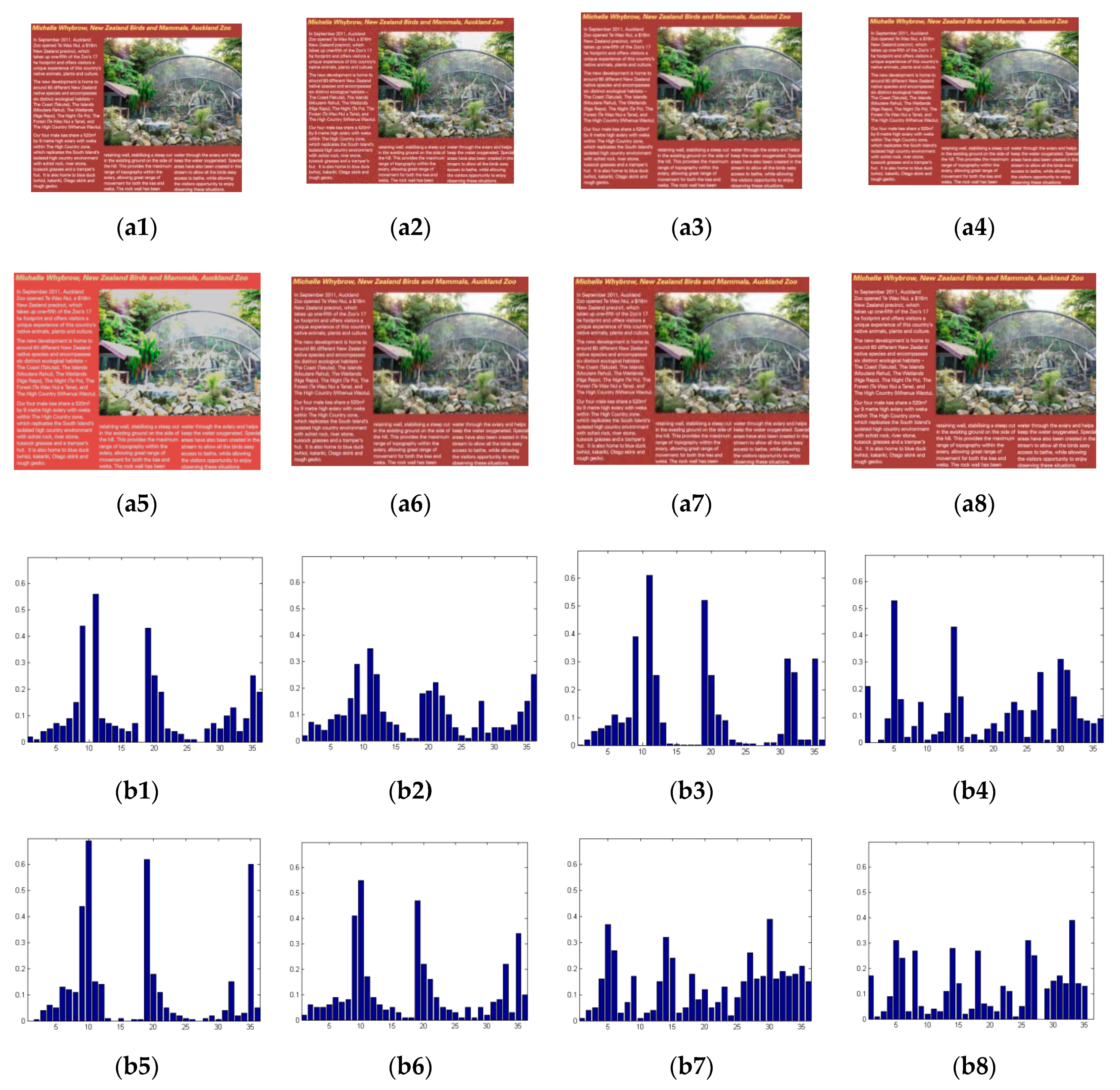
Similarly, we calculate the HOG features of other-order derivatives. In this paper, HOG features of only zero-, first- and second-order derivatives are adopted and HOG features of higher-order derivatives whose orders are greater than two are not adopted. Figure 5 shows the examples of the IHOG features of textual regions. Seven distortion types of distorted SCIs in Figure 5 include Gaussian noise (GN), Gaussian blur (GB), motion blur (MB), contrast change (CC), JPEG compression (JPEG), JPEG2000 compression (JP2K) and layer-segmentation based compression (LSC). In Figure 5, (b1–b8) are the HOG features of the first-order derivative of textual regions contained in corresponding (a1–a8). From (b1–b8) of Figure 5, we can see that textual regions of distorted SCIs with different distortion types result in different IHOG features. Thus, the IHOG features have the discriminative ability for different distortion types.

In this paper, the total IHOG features F_T of textual regions of an SCI are derived as

$$F_T=\left[h_{a,j}^0,h_{a,j}^1,h_{a,j}^2;j=1,2,\dots ,36\right]$$

(7)

where $h_{a,j}^0$, $h_{a,j}^1$ and $h_{a,j}^2$ denote the jth HOG features of zero-, first- and second-order derivatives, respectively.

2.3. Feature Extraction of Pictorial Regions

In this paper, the detailed process of the feature extraction of pictorial regions is depicted in Figure 6. Here, the features of texture variation in both the spatial and shearlet domains are used as structural features of pictorial regions. Additionally, the luminance information is also used as the complementary feature of pictorial regions.

2.3.1. Texture Features of Pictorial Regions in the Spatial Domain

Human vision is very sensitive to the texture variation of an image and so the texture feature should be considered adequately in an IQA model. Generally, the LBP, which can encode the pristine microstructures of an image, is used as the local texture descriptor of an image [43]. However, the LBP has two evident drawbacks: first, in the coding principle of the LBP, the code of a pixel does not consider the directional information of local image structures; second, the LBP is only the first-order derivative pattern and it does not contain the more detailed discriminative information from high-order derivatives. Thus, the application of the LBP in the IQA model will result in comparatively poor predictive performance. To overcome these two drawbacks, Zhang et al. [41], presented the local derivative pattern (LDP), which can describe the local structural primitives of an image by extracting more detailed texture features from high-order derivatives in four directions. In [44,45], the LDP is adopted to construct the FR IQA model. Inspired by the above literature, in the proposed NR BSRSF method, the LDP is introduced to extract the discriminative texture features of pictorial regions in the spatial domain. The detailed extraction process of texture features in the spatial domain is illustrated in Figure 6.

The formula of the LDP is defined as

$$LD{P}_{\theta }^n\left(p\right)={\displaystyle \sum }_{i=0}^{N_A-1}f\left(G_{\theta }^{n-1}\left(p\right)\times G_{\theta }^{n-1}\left(p_i\right)\right)2^i$$

(8)

$$f\left(G_{\theta }^{n-1}\left(p\right)\times G_{\theta }^{n-1}\left(p_i\right)\right)=\{\begin{array}{c}0,\hspace{1em}{G}_{\theta }^{n-1}\left(p\right)\times G_{\theta }^{n-1}\left(p_i\right)\ge 0\\ 1,\hspace{1em}{G}_{\theta }^{n-1}\left(p\right)\times G_{\theta }^{n-1}\left(p_i\right)<0\end{array}$$

(9)

where $LD{P}_{\theta }^n\left(p\right)$ denotes the nth-order LDP value of the pixel $p$ along the direction θ whose values include $0°$, $45°$, $90°$ and $135°$; N_A represents the number of pixels which are adjacent to the pixel $p$; $G_{\theta }^{n-1}\left(p\right)$ and $G_{\theta }^{n-1}\left(p_i\right)$ stands for (n − 1)th-order derivative values of the pixel p and the ith pixel p_i which is adjacent to the pixel p, respectively; and f is a binary function. In (8), the nth-order LDP is coded by using (n − 1)th-order derivative values. Additionally, the LBP can be considered to be a form of the first-order derivative of the LDP.

Here, the statistical distributions of the LDP, namely the histograms of the LDP, are used as feature descriptors. After calculating the LDP code of each pixel of pictorial regions, we calculate the occurrence histograms of the LDP as follows:

$$H_{n,\theta ,k}^{LDP}=\frac{1}{N_P}{\displaystyle \sum }_{p=1}^{N_P}f\left(LD{P}_{\theta }^n\left(p\right),B\left(k\right)\right)$$

(10)

$$f\left(LD{P}_{\theta }^n\left(p\right),B\left(k\right)\right)=\{\begin{array}{c}1,\hspace{1em}LD{P}_{\theta }^n\left(p\right)\in B\left(k\right)\hfill \\ 0,\hspace{1em}\mathrm{otherwise}\hfill \end{array}$$

(11)

where $H_{n,\theta ,k}^{LDP}$ denotes the value of the kth bin in the histogram of the nth derivative along the direction θ; k stands for the bin index of this histogram and its value varies from 1 to 10; n is the derivative index and its value includes 1, 2 and 3; N_P denotes the number of the total pixels in pictorial regions; and $B\left(k\right)$ represents the interval between two adjacent bins in the histogram. When n is equal to 1, θ is meaningless and so $H_{n,\theta ,k}^{LDP}$ is changed into $H_{1,k}^{LDP}$. For each order of LDP along one direction, one histogram with 10 bins can be generated and these bins of this histogram are used as structural features.

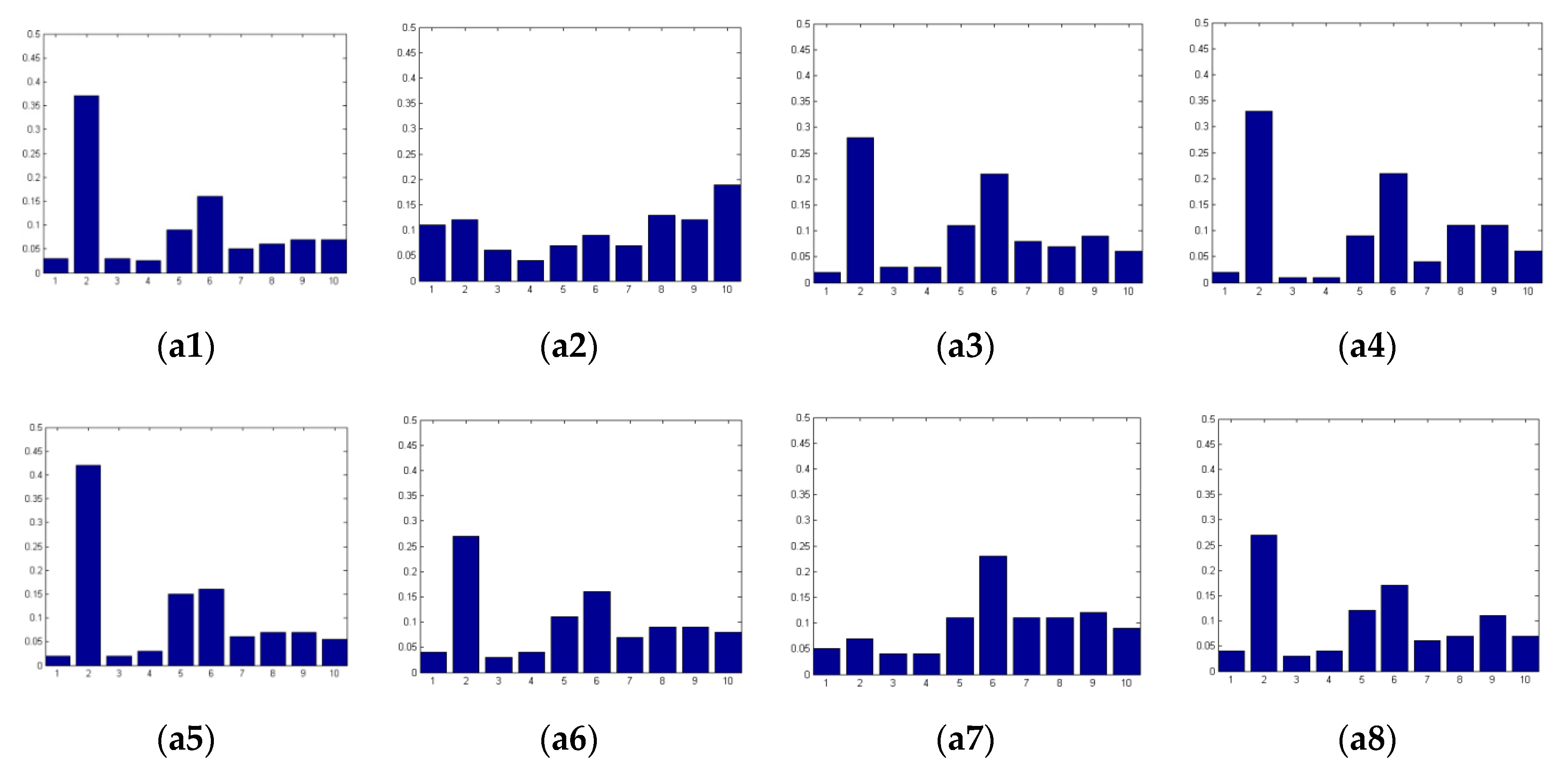
In view of both computational complexity and accuracy, the first three orders of local derivative patterns (LDPs), namely the first-, second- and third-order LDPs, are adopted in the proposed BSRSF method. Since the first-order LDP, namely the LBP, does not consider directional information, the first-order LDP has only one histogram. The second- and third-order LDPs are calculated from four directions so they generate four histograms, respectively. Thus, 90 quality-aware texture features in the spatial domain are generated in the proposed method. Figure 7 shows the examples of the second-order LDP histograms along the direction $0°$. From Figure 7, we can observe that pictorial regions of degraded SCIs with different distortion types can generate different LDP histograms. Consequently, the LDP histograms are discriminative in identifying the distortion types.

In this work, the entire LDP features ${\mathrm{F}}_{\mathrm{P}}^{\mathrm{LDP}}$ of pictorial regions in the spatial domain are obtained as follows:

$${\mathrm{F}}_{\mathrm{P}}^{\mathrm{LDP}}=\left[{\mathrm{H}}_{\mathrm{n},\mathsf{\theta },\mathrm{k}}^{\mathrm{LDP}};\mathrm{n}=1,2,3;\mathsf{\theta }=0°,45°,90°,135°;\mathrm{k}=1,2,\dots ,10\right]$$

(12)

2.3.2. Texture Features of Pictorial Regions in the Shearlet Domain

For picture regions, besides the texture features in the spatial domain, the texture features in the shearlet domain are also employed as structural features in this study. In [14], the generalized local binary pattern (GLBP) operator is proposed to extract texture features from four subband images produced by the Laplacian of Gaussian filters and in the GLBP operator, the central pixel is compared with neighboring pixels by using a threshold. In [15], the wavelet local binary pattern operator is proposed to extract texture features from subbands generated by the wavelet transform. Inspired by these two pattern operators, in this paper, we propose a new texture descriptor called the shearlet local binary pattern (SLBP), which is used to extract texture features from the subbands generated by the shearlet transform. The extraction process of the texture features of pictorial regions in the shearlet domain is shown in Figure 6.

Firstly, the discrete nonseparable shearlet transform (DNST) [46], is applied to pictorial regions of an SCI. The shearlet transform can mimic the multi-channel mechanism of the HVS and has some advantages over the wavelet transform. As the DNST can be regarded as a model of human vision, texture features in the shearlet domain are more discriminative in an IQA model. The formula of the DNST is given as

$$B_{s,d}=\langle S_P,{\psi }_{s,d}\rangle$$

(13)

where $B_{s,d}$ denotes the subband at the sth scale and the dth direction, s represents the scale index, d is the direction index, $S_P$ stands for the gray values of pictorial regions of an SCI and ${\psi }_{s,d}$ denotes the discrete nonseparable shearlet. In this study, the number of scales of the DNST is set to 4 and the numbers of directions in four scales are set to 8, 8, 4 and 4 from finer to coarser scales, respectively. Then, a total of 24 subbands are derived.

Secondly, to extract texture features in the shearlet domain, the SLBP operator is applied to shearlet transform coefficients. Here, for each subband of the DNST, the proposed uniform and rotation invariant SLBP is defined as

$$SLB{P}_{N_C,R,T}^{s,d}\left(c\right)=\{\begin{array}{cc}{\displaystyle {\displaystyle \sum }_{i=0}^{N_C-1}}g\left(B_i-B_c\right),\hfill & \hspace{1em}\mathrm{if} U\left(B_c\right)\le 2\hfill \\ N_C+1,\hfill & \hspace{1em}\mathrm{otherwise}\hfill \end{array}$$

(14)

$$g\left(B_i-B_c\right)=\{\begin{array}{cc}1,\hfill & \left(B_i-B_c\right)\ge T\hfill \\ 0,\hfill & \left(B_i-B_c\right)<T\hfill \end{array}$$

(15)

$$U\left(B_c\right)=\left|g\left(B_{N_C-1}-B_c\right)-g\left(B_0-B_c\right)\right|+{\displaystyle \sum }_{i=1}^{N_C-1}\left|g\left(B_i-B_c\right)-g\left(B_{i-1}-B_c\right)\right|$$

(16)

where $SLB{P}_{N_C,R,T}^{s,d}\left(c\right)$ represents the SLBP value of the coefficient $c$ in the subband at the sth scale and the dth direction; N_C denotes the quantity of the coefficients which are adjacent to the coefficient B_c; R is the radius of the neighborhood of the coefficient $c$; B_c and B_i stand for the intensity values of the central coefficient c and the ith adjacent coefficient, respectively; $g$ denotes a binary function; T represents a threshold value; and $U\left(B_c\right)$ is the uniform pattern of the SLBP. Here, $N_C$ and R are set to 4 and 1, respectively; T has three values, namely −2, 0 and 5. Then, for each value of T, $SLB{P}_{A,R,T}^{s,d}\left(c\right)$ generates six results which vary from 0 to 5.

Finally, the histogram of the SLBP is calculated as

$$H_{s,d,T,k}^{SLBP}=\frac{1}{N_S}{\displaystyle \sum }_{c=1}^{N_S}f\left(SLB{P}_{A,R,T}^{s,d}\left(c\right),k\right)$$

(17)

$$f\left(SLB{P}_{A,R,T}^{s,d}\left(c\right),k\right)=\{\begin{array}{cc}1,\hfill & SLB{P}_{A,R,T}^{s,d}\left(c\right)=k \hfill \\ 0,\hfill & \mathrm{otherwise}\hfill \end{array}$$

(18)

where $H_{s,d,T,k}^{SLBP}$ denotes the value of the kth bin in the histogram of the subband at the sth scale and the dth direction in which the threshold T is used, k ranges from 0 to 5 and N_S represents the number of the total coefficients in this subband. For one value of the threshold T, we can obtain one histogram with six bins from one subband and these six bins of this histogram are used as structural features. Since 24 subbands are generated and the threshold T with three values is used for each subband in the proposed BSRSF method, we can obtain 72 histograms.

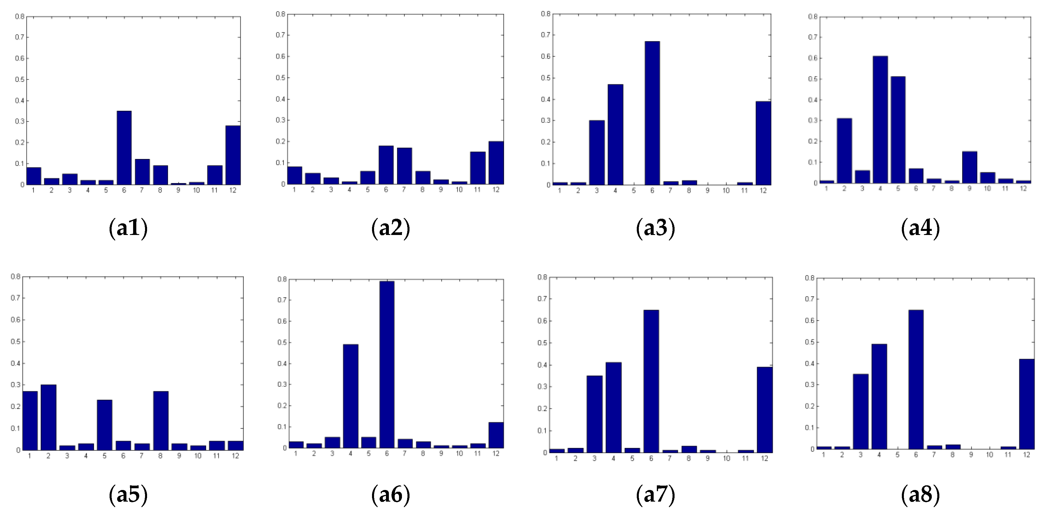
Figure 8 shows the examples of texture features of pictorial regions in the shearlet domain. Each subgraph of (a1–a8) of Figure 8 contains two concatenated SLBP histograms calculated from the two DNST subbands at the first scale and the first and second directions. From Figure 8, we can observe that pictorial regions of distorted SCIs with different distortion types can produce different SLBP histograms. So, the SLBP histograms are discriminative in categorizing distortion types.

All of the SLBP features $F_P^{SLBP}$ of pictorial regions are obtained as

$$F_P^{SLBP}=\left[H_{s,d,T,k}^{SLBP};T=-2,0,5;k=0,1,\dots ,5\right]$$

(19)

2.3.3. Luminance Features of Pictorial Regions

Besides the texture information of an image, human vision also has high sensitivity to the luminance variation of an image which can induce obvious distortions and so the luminance features also have a high correlation with the perceptual quality of an image. In this study, the luminance information is used as the complementary feature of pictorial regions. In [11], the distribution of MSCN values is modeled approximately by the generalized Gaussian function (GGF), the distributions of pairwise products of the neighboring MSCN values in four directions are modeled approximately by the asymmetric generalized Gaussian function (AGGF) and 18 parameters of GGF and AGGF are adopted as luminance features of the image. However, this feature representation method has a drawback that fitting errors will inevitably be produced by this approximate modeling method. To overcome this drawback, in this paper, the statistical histogram is adopted as the representation form of the luminance information since the histogram does not produce fitting errors. The calculation process of luminance histograms is illustrated in Figure 6. To be specific, the histograms of MSCN values and four pairwise products of neighboring MSCN values are used as the luminance features of pictorial regions. Additionally, we also consider the statistical information from the local average values and local contrast values of pictorial regions. Local average values can mimic the point spread function of the optics in human eyes and local contrast values have a close relationship with the image quality. Likewise, their histograms are calculated as luminance features. The MSCN operation is conducted as follows:

$$S_P^M\left(x,y\right)=\frac{S_P\left(x,y\right)-S_P^A\left(x,y\right)}{S_P^{\sigma }\left(x,y\right)+c}$$

(20)

where $S_P^M\left(x,y\right)$ denotes the MSCN value; $S_P\left(x,y\right)$ represents the gray values of pictorial regions; $S_P^A\left(x,y\right)$ and $S_P^{\sigma }\left(x,y\right)$ denote the local average value and local contrast value in a 7 × 7 neighborhood centered on (x, y), respectively; and c represents a constant and is set to 1. $S_P^A\left(x,y\right)$ and $S_P^{\sigma }\left(x,y\right)$ are computed as

$$S_P^A\left(x,y\right)={\displaystyle \sum }_{m=-3}^3{\displaystyle \sum }_{n=-3}^3{\omega }_{m,n}{S}_P\left(x+m,y+n\right)$$

(21)

$$S_P^{\sigma }\left(x,y\right)=\sqrt{{\displaystyle \sum }_{m=-3}^3{\displaystyle \sum }_{n=-3}^3{\omega }_{m,n}{\left(S_P\left(x+m,y+n\right)-S_P^A\left(x,y\right)\right)}^2}$$

(22)

where $\left\{{\omega }_{m,n}\right|m=-3,\dots 3;n=-3,\dots 3\}$ denotes a set of unit-volume Gaussian weights.

Four pairwise products $S_P^H\left(x,y\right)$, $S_P^V\left(x,y\right)$, $S_P^{D_1}\left(x,y\right)$ and $S_P^{D_2}\left(x,y\right)$ of the MSCN values along four different directions in a 3 × 3 neighborhood are computed as

$$S_P^H\left(x,y\right)=S_P^M\left(x,y\right)S_P^M\left(x,y+1\right)$$

(23)

$$S_P^V\left(x,y\right)=S_P^M\left(x,y\right)S_P^M\left(x+1,y\right)$$

(24)

$$S_P^{D_1}\left(x,y\right)=S_P^M\left(x,y\right)S_P^M\left(x+1,y+1\right)$$

(25)

$$S_P^{D_2}\left(x,y\right)=S_P^M\left(x,y\right)S_P^M\left(x+1,y-1\right)$$

(26)

For MSCN values, four pairwise products, local average values and local contrast values, their absolute values are calculated first and then their statistical histograms are computed as

$$H_{W,k}^L=\frac{1}{N_P}{\displaystyle \sum }_{\left(x,y\right)}f\left(\left|S_P^W\left(x,y\right)\right|,B\left(k\right)\right)$$

(27)

$$f\left(\left|S_P^W\left(x,y\right)\right|,B\left(k\right)\right)=\{\begin{array}{cc}1,\hfill & \left|S_P^W\left(x,y\right)\right|\in B\left(k\right)\hfill \\ 0,\hfill & \mathrm{otherwise}\hfill \end{array}$$

(28)

where $H_{W,k}^L$ denotes the value of the kth bin of the histogram; k stands for the bin index of the histogram and its value varies from 1 to 10; N_P represents the number of pixels in pictorial regions; $B\left(k\right)$ is the interval between two neighboring bins in the histogram; and W denotes the type index of the histograms. The value of W includes M, A, σ, H, v, D₁ and D₂. M, A and σ stand for MSCN values, local average values and local contrast values, respectively. H, v, D₁ and D₂ represent four pairwise products of MSCN values. In this way, each histogram generates 10 bins which are employed as luminance features.

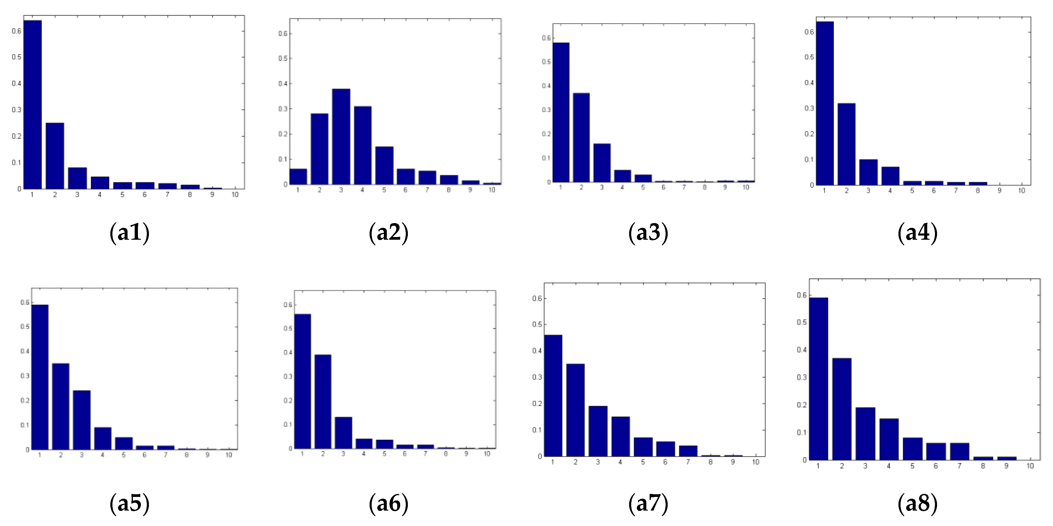
Figure 9 illustrates the examples of luminance features of pictorial regions. Each subgraph of (a1–a8) of Figure 9 contains the histogram of MSCN values of pictorial regions contained in distorted SCIs caused by different distortion types. From Figure 9, we can observe that different histograms of MSCN values are produced for pictorial regions of distorted SCIs with different distortion types. Thus, luminance features are effective to characterize the quality degradation of pictorial regions of degraded SCIs caused by different distortion types.

The entire luminance features $F_P^L$ of pictorial regions of an SCI are derived as

$$F_P^L=\left[H_{W,k}^L;W=M,A,\sigma ,H,v,D_1,D_2;k=1,2,\dots ,10\right]$$

(29)

Finally, the entire features $F_P$ of pictorial regions of an SCI are derived by combining structural features and luminance features as

$$F_P=\left[F_P^{LDP},F_P^{SLBP}, F_P^L\right]$$

(30)

2.4. Regression Models

In this paper, the SVR-based machine learning technique is adopted to implement the complex nonlinear mapping relationship between quality-aware features and subjective evaluation values, which has been depicted in Figure 2. The SVR is frequently used to pool high-dimensional data. The predictive value $Q_T$ of textual regions of an SCI is calculated as

$$Q_T=Fu{n}_T\left(F_T\right)$$

(31)

where F_T denotes the features of textual regions of this SCI which are extracted in (7) and Fun_T represents a regression model which has been trained beforehand by employing the SVR. Here, the ε-SVR [47] is used to conduct the regression model learning and Fun_T is given as

$$Fu{n}_T\left(x\right)={\displaystyle \sum }_{j=1}^J\left({\beta }_j-{\beta }_j^{*}\right)K\left(x_j, x\right)+b$$

(32)

$$K\left(x_j, x\right)=e^{-\rho {\left|\left|x_j-x\right|\right|}^2}$$

(33)

where ${\beta }_j$ and ${\beta }_j^{*}$ ($0\le {\beta }_j$, ${\beta }_j^{*}\le C$) denote the Lagrange multipliers, C represents the tradeoff error parameter, b is a bias parameter, J represents the number of support vectors, x_j denotes the jth support vector, x denotes the feature vector of textual regions, $K\left(x_j, x\right)$ is a radial basis function (RBF) kernel and $\rho$ denotes the width of the RBF kernel. More detail about the ε-SVR can be found in [47].

Similarly, we can derive the predictive value $Q_P$ of pictorial regions of an SCI as

$$Q_P=Fu{n}_P\left(F_P\right)$$

(34)

where F_P represents the features of pictorial regions of SCIs extracted in (30) and Fun_P denotes the trained regression model.

2.5. Weighting Combination

Above, we obtain the predictive values of textual and pictorial regions of an SCI. To derive the overall predictive value of this SCI, in this study, we propose an activity weighting strategy to fuse the predictive values of textual and pictorial regions and this strategy is based on the properties of human vision. In general, human vision has greater sensitivity to the high-frequency content (for example, edges and textures) than the background content with slight variation in an image. Thus, the degradation of the high-frequency content is easier to find by human vision than the background content. In this study, to quantify the high-frequency characteristic in an SCI, the activity measure of the gradient map of this SCI is adopted.

The activity measure can describe the change degree of the image content [19]. Here, the activity measure map $A\left(x,y\right)$ of an image $f\left(x,y\right)$ is defined as

$$A\left(x,y\right)=\gamma V_1\left(x,y\right)+\left(1-\gamma \right)V_2\left(x,y\right)$$

(35)

where $V_1\left(x,y\right)$ denotes the one-distance variation in diagonal orientations; $V_2\left(x,y\right)$ represents the two-distance change in the horizontal and vertical orientations; and $\gamma$ stands for a weighting coefficient to tune the combination of $V_1\left(x,y\right)$ and $V_2\left(x,y\right)$. In [19], the optimum performance of the activity measure can be achieved when $\gamma$ ranges from 0.3 to 0.5. More detail about $\gamma$ can be found in [19]. In this paper, $\gamma$ is set to 0.4. $V_1\left(x,y\right)$ and $V_2\left(x,y\right)$ are defined as

$$\begin{array}{c}{V}_1\left(x,y\right)={\left(f\left(x,y\right)-f\left(x-1,y-1\right)\right)}^2+{\left(f\left(x,y\right)-f\left(x+1,y+1\right)\right)}^2\\ +{\left(f\left(x,y\right)-f\left(x-1,y+1\right)\right)}^2+{\left(f\left(x,y\right)-f\left(x+1,y-1\right)\right)}^2\end{array}$$

(36)

$$V_2\left(x,y\right)={\left(f\left(x-1,y-1\right)-f\left(x+1,y+1\right)\right)}^2+{\left(f\left(x-1,y+1\right)-f\left(x+1,y-1\right)\right)}^2$$

(37)

In this paper, the Prewitt filter is used first to compute the gradient map of textual and pictorial regions via (3) and $M^1\left(x,y\right)$ in (3) denotes this gradient map. Secondly, we compute the activity measure maps $A_T^G\left(x,y\right)$ and $A_P^G\left(x,y\right)$ of the gradient maps of textual and pictorial regions via (35), respectively. Finally, in this paper, the predictive value $Q$ of a distorted SCI is defined as

$$Q=\frac{1}{A_T^{M,G}+A_P^{M,G}}(A_T^{M,G}{Q}_T+A_P^{M,G}{Q}_P)$$

(38)

where $Q_T$ and $Q_P$ denote, respectively, the predictive values of textual and pictorial regions calculated in (31) and (34); and $A_T^{M,G}$ and $A_P^{M,G}$ represent the mean activity measure values of the gradient maps of textual and pictorial regions in this SCI, respectively. $A_T^{M,G}$ and $A_P^{M,G}$ are defined as

$$A_T^{M,G}=\frac{1}{N_T^G}{\displaystyle \sum }_{n=1}^{N_T}{A}_T^G\left(x,y\right)$$

(39)

$$A_P^{M,G}=\frac{1}{N_P^G}{\displaystyle \sum }_{n=1}^{N_P}{A}_P^G\left(x,y\right)$$

(40)

where $N_T^G$ and $N_P^G$ denote the numbers of pixels in the gradient maps of textual and pictorial regions, respectively.

3. Experimental Results

3.1. Experimental Protocol

To validate the advantages of the proposed BSRSF method, comparison experiments are made on the two SCI databases SIQAD [18], and SCID [21]. The SIQAD includes 20 original SCIs and 980 impaired SCIs caused by seven degradation types and seven degradation levels. These seven degradation types comprise GN, GB, MB, CC, JPEG, JP2K and LSC. The SCID consists of 40 raw SCIs and 1800 degraded SCIs. For each raw SCI in the SCID, nine degradation types and five degradation levels are applied and these degradation types include GN, GB, MB, CC, JPEG, JP2K, color saturation change (CSC), color quantization with dithering (CQD) and high-efficiency video coding (HEVC).

Here, three generally employed criteria are used to evaluate the predictive ability of IQA models: the Pearson linear correlation coefficient (PLCC), Spearman rank-order correlation coefficient (SROCC) and root mean squared error (RMSE). PLCC and SROCC are used to test the predictive accuracy and monotonicity, respectively. RMSE is used to test the predictive consistency. If an IQA model can simultaneously derive larger PLCC and SROCC values and smaller RMSE values, this model achieves better predictive performance. Since the predictive values generated from different IQA models have diverse dynamic scopes, in this paper, a mapping function is used to map predictive values into a uniform scope:

$$f\left(v\right)={\alpha }_1\left(0.5-\frac{1}{1+e^{\left({\alpha }_2\left(v-{\alpha }_3\right)\right)}}\right)+{\alpha }_{4}v+{\alpha }_5$$

(41)

where $v$ denotes a predictive value, $f\left(v\right)$ represents the mapped predictive value and $\left({\alpha }_1,{\alpha }_2, \dots , {\alpha }_5\right)$ stand for the parameters to be fitted.

3.2. Performance Comparison Experiments

In this study, the proposed BSRSF method is compared with the following existing IQA models: PSNR, SSIM [3], GMSD [6], SPQA [18], ESIM [21], SFUW [20], SQI [48], RRSCI [25], BRISQUE [11], GWH-GLBP [13], IL-NIQE [16], BQMS [28], SIQE [17], NRLT [33] and BLIQUP-SCI [29]. Among these models, PSNR, SSIM, GMSD, SPQA, ESIM, SFUW and SQI are FR IQA models, RRSCI is an RR IQA model and BRISQUE, GWH-GLBP, IL-NIQE, BQMS, SIQE, NRLT and BLIQUP-SCI are blind IQA models. Additionally, SPQA, ESIM, SFUW, SQI, RRSCI, BQMS, SIQE, NRLT and BLIQUP-SCI have been specifically devised to evaluate the quality of SCIs.

For three FR metrics SPQA, SQI and SFUW, and one RR metric RRSCI, the experimental results are directly obtained from their references. For the rest of the FR metrics, the results are calculated by running the source codes provided by their authors. For the blind metrics, the results of BLIQUP-SCI are directly taken from its reference. For the rest of the blind metrics, their source codes are used to derive experimental results. For the proposed BSRSF metric and learning-based blind metrics including BRISQUE, GWH-GLBP, IL-NIQE, BQMS, SIQE and NRLT, an SCI database is randomly split into two subsets: the training subset and the evaluation subset. The training subset includes 80% SCIs of this database and the evaluation subset includes 20% SCIs of this database. The distorted SCIs in the training subset are used to train the model and then this trained model is used to evaluate the quality of distorted SCIs in the evaluation subset. This train–evaluate operation is repeated 1000 times on this database and the median experimental results across 1000 train-evaluate operations are reported. In the proposed metric, the LibSVM package [49], is employed as the SVR tool. When the ε-SVR is employed to learn the regression models, two parameters (C, $\rho$) of the ε-SVR need to be decided. In our experiments, a grid search in the logarithm space is used to estimate the optimal values of C and $\rho$ [47]. For the regression model of textual regions of SCIs, the optimal values of (C, $\rho$) are found to be (16,384, 2) and (256, 16) on SIQAD and SCID, respectively. For the regression model of pictorial regions of SCIs, the optimal values of (C, $\rho$) are found to be (8192, 4) and (512, 0.5) on SIQAD and SCID, respectively. Experimental results are tabulated in

Table 1. Performance comparison of the proposed BSRSF model and full-reference (FR) models.

Databases	Criteria	PSNR	SSIM	GMSD	SPQA	ESIM	SQI	SFUW	BSRSF
SIQAD	PLCC	0.5869	0.7561	0.7259	0.8584	0.8788	0.8644	0.8910	0.8905
	SROCC	0.5605	0.7566	0.7305	0.8416	0.8632	0.8548	0.8800	0.8714
	RMSE	11.5876	9.3676	9.4684	7.3421	6.8310	7.1782	6.4990	7.2569
SCID	PLCC	0.7622	0.7343	0.8337	-	0.8630	-	0.8590	0.7024
	SROCC	0.7512	0.7146	0.8138	-	0.8478	-	0.8950	0.7204
	RMSE	9.1682	9.6133	7.8210	-	7.1552	-	7.3100	9.8849

and

Table 2. Performance comparison of the proposed BSRSF model and reduced-reference (RR) and blind models.

Databases	Criteria	RRSCI	BRISQUE	GWH-GLBP	IL- NIQE	BQMS	SIQE	NRLT	BLIQUP- SCI	BSRSF
SIQAD	PLCC	0.8014	0.7684	0.7903	0.3996	0.8108	0.7905	0.8387	0.7705	0.8905
	SROCC	0.7655	0.7094	0.7233	0.3496	0.7619	0.7609	0.8197	0.7990	0.8714
	RMSE	8.5620	8.2565	8.7480	13.2082	9.3110	8.7775	7.5847	10.0200	7.2569
SCID	PLCC	0.6602	0.6137	0.6468	0.2569	0.6338	0.6457	0.6324	-	0.7024
	SROCC	0.7526	0.5795	0.6348	0.2432	0.6132	0.6022	0.6387	-	0.7204
	RMSE	11.5401	12.2565	12.2831	13.6863	10.9519	10.9343	10.6327	-	9.8849

, and the best two results of each row are highlighted in boldface. Furthermore, as the papers of SPQA, SQI and BLIQUP-SCI do not provide the experimental results for SCID, these results are absent in these two tables.

From Table 1, we can draw three conclusions. Firstly, the proposed NR BSRSF method has a competitive predictive ability in comparison to the FR SCI evaluation methods which include SPQA, ESIM, SQI and SFUW; meanwhile, it achieves preferable performance in contrast with the traditional FR natural image evaluation methods which include PSNR, SSIM and GMSD. Secondly, for SCIs, the four dedicated SCI evaluation models which include SPQA, ESIM, SQI and SFUW achieve better performance than the traditional IQA models which include PSNR, SSIM and GMSD. The reason for this is that these dedicated models carefully deal with the distinctions between the visual characteristics of textual and pictorial regions in SCIs, while traditional IQA methods equally consider the visual characteristics of textual and pictorial content in SCIs. Finally, among these FR methods, ESIM and SFUW are the top two prediction methods.

From Table 2, it is clear that the designed NR BSRSF model achieves the maximal PLCC and SROCC scores and the minimum RMSE score on the two SCI databases. For SIQAD, the BSRSF method achieves, respectively, improvements of 6.2% and 6.3% against the other top blind method (NRLT) for PLCC and SROCC; meanwhile, it achieves an improvement of 4.3% against the other top blind method (NRLT) for RMSE. For SCID, the BSRSF method also derives similar experimental results. These results indicate that the proposed BSRSF method attains the best predictive ability among the compared blind and RR methods. Furthermore, the natural image evaluation methods which include BRISQUE, GWH-GLBP and IL-NIQE are weak in terms of evaluating the quality of a distorted SCI, because these methods do not carefully consider the features of the textual content in SCIs. In particular, IL-NIQUE delivers the worst predictive ability among all of the compared methods and the reason for this is that the NSS features employed in IL-NIQUE are unsuitable to represent the visual perception of distorted SCIs.

3.3. Performance Comparison for Different Distortion Categories

To completely evaluate the predictive capability of the proposed BSRSF method for the distorted SCIs induced by different distortion types, we conduct comparison experiments of the BSRSF method and other methods on seven distortion types of the SIQAD database. The experimental results, namely the PLCC scores, are listed in

Table 3. PLCC scores of metrics for seven degradation types in SIQAD.

Metrics		GN	GB	MB	CC	JPEG	JP2K	LSC
FR Metrics	PSNR	0.9053	0.8603	0.7044	0.7401	0.7545	0.7893	0.7805
	SSIM	0.8806	0.9014	0.8060	0.7435	0.7487	0.7749	0.7307
	GMSD	0.8956	0.9094	0.8436	0.7827	0.7746	0.8509	0.8559
	SPQA	0.8921	0.9058	0.8315	0.7992	0.7696	0.8252	0.7958
	ESIM	0.8891	0.9234	0.8886	0.7641	0.7999	0.7888	0.7915
	SQI	0.8829	0.9202	0.8789	0.7724	0.8218	0.8271	0.8310
	SFUW	0.8870	0.9230	0.8780	0.8290	0.7570	0.8150	0.7590
RR Metrics	RRSCI	0.8798	0.8810	0.8465	0.6812	0.7638	0.6807	0.7110
Blind Metrics	BRISQUE	0.8423	0.8247	0.7783	0.5548	0.7018	0.6823	0.5615
	GWH-GLBP	0.8537	0.8917	0.8297	0.4973	0.5687	0.7043	0.5678
	IL-NIQE	0.7667	0.5304	0.4136	0.1171	0.2945	0.4172	0.1754
	BQMS	0.8353	0.8048	0.6969	0.5125	0.6686	0.7059	0.6562
	SIQE	0.8590	0.8531	0.7817	0.5905	0.7639	0.7637	0.7752
	NRLT	0.9101	0.8903	0.8865	0.7994	0.7851	0.7035	0.7219
	BLIQUP-SCI	0.9015	0.9453	0.6341	0.7278	0.6691	0.6001	0.4253
	BSRSF	0.9307	0.9405	0.9364	0.7807	0.8547	0.8554	0.8701

. For each distortion type, three optimal PLCC scores in this table are indicated in boldface. On the basis of the experimental results in this table, we can draw two conclusions. Firstly, compared with other methods, the proposed BSRSF method obtains preferable experimental results for the majority of distortion types. To be more specific, the BSRSF method can derive accurate assessment results for six distortion types: GN, GB, MB, JPEG, JP2K and LSC. The reason for this is that the blur and compression can change the local structures of SCIs and the features used by the BSRSF method can precisely denote the degradation degree of local structures. Secondly, for the distortion type CC, the BSRSF method obtains a comparable PLCC score compared to the other top-three methods. In short, for different distortion types, the proposed BSRSF metric achieves better or clearly competitive predictive capability compared to other metrics, which further validates the robustness of the BSRSF metric.

3.4. Statistical Significance Comparison

To further validate the advantages of the proposed BSRSF metric against other blind metrics, we compare the statistical significance of the BSRSF metric and other blind metrics. In this study, we perform F-tests on the SROCC scores derived by these metrics. F-tests are carried out at the 5% significance level. The experimental results on SIQAD are listed in

Table 4. Experimental results of F-tests on SIQAD.

Metrics	BRISQUE	GWH-GLBP	IL-NIQE	BQMS	SIQE	NRLT	BLIQUP-SCI	BSRSF
BRISQUE	0	1	1	−1	−1	−1	−1	−1
GWH-GLBP	−1	0	1	−1	−1	−1	−1	−1
IL-NIQE	−1	−1	0	−1	−1	−1	−1	−1
BQMS	1	1	1	0	0	−1	−1	−1
SIQE	1	1	1	0	0	−1	1	−1
NRLT	1	1	1	1	1	0	0	−1
BLIQUP-SCI	1	1	1	1	−1	0	0	−1
BSRSF	1	1	1	1	1	1	1	0

, where “1” shows that the row method outperforms the column method in terms of statistical significance, “−1” shows that the contrary meaning and “0” shows that the row and column methods are not distinguishable in terms of statistical significance. From Table 4, we can observe that all comparison results of the BSRSF method to other compared methods are marked with “1”. Thus, the BSRSF method completely statistically exceeds all compared blind methods.

3.5. Order Selection of Derivatives of IHOG Features Used in Textual Regions

As mentioned above, the IHOG features of the multi-order derivatives are adopted as structural features of textual regions of an SCI. Here, we investigate which combination method of HOG features of the different-order derivative is optimal for structural features of textual regions.

Table 5. Experimental results of the order selection of derivatives for IHOG features on SIQAD.

Criteria	Com-0	Com-1	Com-2	Com-3	Com-4	Com-5
PLCC	0.8654	0.8801	0.8905	0.8865	0.8805	0.8795

listed the experimental results of the order selection of derivatives used in the IHOG features on SIQAD. In Table 5, “Com-0” denotes that the HOG features of only the zero-order derivative are used, “Com-1” denotes that the HOG features of zero- and first-order derivatives are adopted, “Com-2” denotes that the HOG features of zero-, first- and second-order derivatives are used, “Com-3” denotes that the HOG features of zero-, first-, second- and third-order derivatives are used, “Com-4” denotes that the HOG features of zero-, first-, second-, third- and fourth-order derivatives are used and “Com-5” denotes that the HOG features of zero-, first-, second-, third-, fourth- and fifth-order derivatives are used. Figure 10 shows the curve of PLCC values for different combinations of HOG features. From Table 5 and Figure 10, we can observe that the PLCC value gradually increases from “Com-0” to “Com-2” while the PLCC value gradually decreases from “Com-2” to “Com-5”. Among the five combination methods, “Com-2” achieves the maximal PLCC value. According to the experimental results, we select “Com-2” as the final combination method. Namely, in this paper, the HOG features of zero-, first- and second-order derivatives are adopted as structural features of textual regions.

3.6. Effect of Features from Textual and Pictorial Regions

The quality-aware features used by the proposed BSRSF metric are derived from two kinds of regions in SCIs: textual and pictorial regions. To investigate the impact of the employed features from textual and pictorial regions in the BSRSF metric, we devised two metrics: Metric-T and Metric-P. Metric-T uses only the features of textual regions and does not use the features of pictorial regions. The predictive value $Q_T$ for textual regions in (31) is used as the final assessment value of Metric-T. On the contrary, Metric-P adopts only the features of pictorial regions and discards the features of textual regions. The predictive value $Q_P$ of pictorial regions in (34) is used as the final assessment value of Metric-P. Here, the BSRSF metric is compared with these two metrics and the experimental results on SIQAD are listed in

Table 6. Effects of features from textual and pictorial regions on SIQAD.

Criteria	Metric-T	Metric-P	BSRSF
PLCC	0.8727	0.7829	0.8905
SROCC	0.8524	0.7684	0.8714
RMSE	7.7843	8.3547	7.2569

.

From Table 6, two conclusions can be drawn. Firstly, the BSRSF metric employing the features from two kinds of regions achieves better predictive ability than Metric-T and Metric-P, which employ features from only one kind of region. This indicates that, to improve the performance of the quality evaluation method of SCIs, it is necessary to simultaneously deal with the features from the two kinds of regions. Secondly, the performance of Metric-T is much better than that of Metric-P, which shows that the features of textual regions are more important than those of pictorial regions. Certainly, the features of pictorial regions have an indispensable effect for the overall quality evaluation of SCIs.

4. Conclusions

In this work, we put forward a new blind quality assessment metric of SCIs by considering regionalized structural features. Specifically, the improved histograms of oriented gradients computed from the multi-order derivatives are used as the structural features of textual regions of SCIs, and structural features of pictorial regions of SCIs include LDP histogram features in the spatial domain and SLBP histogram features in the shearlet domain. Additionally, the luminance information is also taken into account as the complementary feature of pictorial regions. The SVR-based scheme is used to incorporate these features and derive the predictive scores of textual and pictorial regions. Furthermore, we devise an activity weighting strategy to fuse the predictive scores of textual and pictorial regions as the final assessment value of the SCI. Experimental results indicate that the proposed BSRSF metric is well coherent with subjective judgments and achieves preferable predictive capability compared to the existing blind metrics for SCIs.

At present, the research work of the NR SCIQA is still in the initial stage and there is still a great deal of room to further optimize and improve the performance of the NR SCIQA methods. Our future studies will focus on the following six directions. Firstly, since the proposed method does not achieve the best predictive performance for the distortion type CC compared to other methods, we will further investigate structural features which are appropriate to the distortion type CC. Structural features of SCIs should be explored in more depth from the perspective of human physiology and psychology. Secondly, since subjective evaluation values are still needed to train the regression models in the proposed method, we will investigate a completely blind quality assessment method of SCIs in which subjective ratings values can be omitted. Thirdly, since both the segmentation of SCIs and the calculation of multiple features of textual and pictorial regions increase the computational complexity of the proposed method, the proposed method may be not suitable for real-time applications and so we will further improve the efficiency of the proposed method and simultaneously retain the effectiveness of the proposed method. Fourthly, more appropriate machine learning techniques, such as deep learning approaches, will be devised to further improve the predictive accuracy of the evaluation method. Deep learning approaches have been widely applied in many fields which include speech recognition, natural language processing, audio recognition and bioinformatics, and have already achieved satisfactory performance. Fifthly, we plan to develop a unified model that can simultaneously perform the faithful quality evaluation of SCIs and natural images. Finally, we will investigate the quality assessment of color SCIs and screen content videos (SCVs). Perceptual chrominance features should be considered adequately in quality evaluation models of color SCIs. Additionally, although the natural videos quality assessment methods have been extensively investigated in the past decades, studies of the quality assessment of SCVs have still not been carried out until now.

References

- Wang, S.; Ma, L.; Fang, Y.; Lin, W.; Ma, S.; Gao, W. Just noticeable difference estimation for screen content images. IEEE Trans. Image Process. 2016, 25, 3838–3851. [Google Scholar] [CrossRef] [PubMed]
- Bai, Y.; Yu, M.; Jiang, Q.; Jiang, G.; Zhu, Z. Learning content-specific codebooks for blind quality assessment of screen content images. Signal Process. 2019, 161, 248–258. [Google Scholar] [CrossRef]
- Wang, Z.; Bovik, A.C.; Sheikh, H.R.; Simoncelli, E.P. Image quality assessment: From error visibility to structural similarity. IEEE Trans. Image Process. 2004, 13, 600–612. [Google Scholar] [CrossRef] [PubMed] [Green Version]
- Zhang, L.; Zhang, L.; Mou, X.; Zhang, D. FSIM: A feature similarity index for image quality assessment. IEEE Trans. Image Process. 2011, 20, 2378–2386. [Google Scholar] [CrossRef] [PubMed] [Green Version]
- Sheikh, H.R.; Bovik, A.C. Image information and visual quality. IEEE Trans. Image Process. 2006, 15, 430–444. [Google Scholar] [CrossRef]
- Xue, W.; Zhang, L.; Mou, X.; Bovik, A.C. Gradient magnitude similarity deviation: A highly efficient perceptual image quality index. IEEE Trans. Image Process. 2014, 23, 684–695. [Google Scholar] [CrossRef] [PubMed] [Green Version]
- Wu, J.; Lin, W.; Shi, G.; Liu, A. Perceptual quality metric with internal generative mechanism. IEEE Trans. Image Process. 2013, 22, 43–54. [Google Scholar] [PubMed]
- Gao, F.; Wang, Y.; Li, P.; Tan, M.; Yu, J.; Zhu, Y. Deepsim: Deep similarity for image quality assessment. Neurocomputing 2017, 257, 104–114. [Google Scholar] [CrossRef]
- Golestaneh, S.; Karam, L.J. Reduced-reference quality assessment based on the entropy of DWT coefficients of locally weighted gradient magnitudes. IEEE Trans. Image Process. 2016, 25, 5293–5303. [Google Scholar] [CrossRef]
- Fu, Y.; Wang, S. A no reference image quality assessment metric based on visual perception. Algorithms 2016, 9, 87. [Google Scholar] [CrossRef] [Green Version]
- Mittal, A.; Moorthy, A.K.; Bovik, A.C. No-reference image quality assessment in the spatial domain. IEEE Trans. Image Process. 2012, 21, 4695–4708. [Google Scholar] [CrossRef] [PubMed]
- Li, Q.; Lin, W.; Xu, J.; Fang, Y. Blind image quality assessment using statistical structural and luminance features. IEEE Trans. Multimedia 2016, 18, 2457–2469. [Google Scholar] [CrossRef]
- Li, Q.; Lin, W.; Fang, Y. No-reference quality assessment for multiply-distorted images in gradient domain. IEEE Signal Process. Lett. 2016, 23, 541–545. [Google Scholar] [CrossRef]
- Zhang, M.; Muramatsu, C.; Zhou, X.; Hara, T.; Fujita, H. Blind image quality assessment using the joint statistics of generalized local binary pattern. IEEE Signal Process. Lett. 2015, 22, 207–210. [Google Scholar] [CrossRef]
- Rezaie, F.; Helfroush, M.S.; Danyali, H. No-reference image quality assessment using local binary pattern in the wavelet domain. Multimedia Tools Appl. 2018, 77, 2529–2541. [Google Scholar] [CrossRef]
- Zhang, L.; Zhang, L.; Bovik, A.C. A feature-enriched completely blind image quality evaluator. IEEE Trans. Image Process. 2015, 24, 2579–2591. [Google Scholar] [CrossRef] [Green Version]
- Gu, K.; Zhou, J.; Qiao, J.F.; Zhai, G.; Lin, W.; Bovik, A.C. No-reference quality assessment of screen content pictures. IEEE Trans. Image Process. 2017, 26, 4005–4018. [Google Scholar] [CrossRef]
- Yang, H.; Fang, Y.; Lin, W. Perceptual quality assessment of screen content images. IEEE Trans. Image Process. 2015, 24, 4408–4421. [Google Scholar] [CrossRef]
- Yang, H.; Wu, S.; Deng, C.; Lin, W. Scale and orientation invariant text segmentation for born-digital compound images. IEEE Trans. Cybern. 2015, 45, 533–547. [Google Scholar]
- Fang, Y.; Yan, J.; Liu, J.; Wang, S.; Li, Q.; Guo, Z. Objective quality assessment of screen content image by uncertainty weighting. IEEE Trans. Image Process. 2017, 26, 2016–2027. [Google Scholar] [CrossRef]
- Ni, Z.; Ma, L.; Zeng, H.; Chen, J.; Cai, C.; Ma, K.K. ESIM: Edge similarity for screen content image quality assessment. IEEE Trans. Image Process. 2017, 26, 4818–4831. [Google Scholar] [CrossRef] [PubMed]
- Fu, Y.; Zeng, H.; Ma, L.; Ni, Z.; Zhu, J.; Ma, K.K. Screen content image quality assessment using multi-scale difference of Gaussian. IEEE Trans. Circuits Syst. Video Technol. 2018, 28, 2428–2432. [Google Scholar] [CrossRef]
- Wang, R.; Yang, H.; Pan, Z.; Huang, B.; Hou, G. Screen content image quality assessment with edge features in gradient domain. IEEE Access 2019, 7, 5285–5295. [Google Scholar] [CrossRef]
- Ni, Z.; Zeng, H.; Ma, L.; Hou, J.; Chen, J.; Ma, K.K. A Gabor feature-based quality assessment model for the screen content images. IEEE Trans. Image Process. 2018, 27, 4516–4528. [Google Scholar] [CrossRef] [PubMed]
- Wang, S.; Gu, K.; Zhang, X.; Lin, W.; Ma, S.; Gao, W. Reduced-reference quality assessment of screen content images. IEEE Trans. Circuits Syst. Video Technol. 2018, 28, 1–14. [Google Scholar] [CrossRef]
- Wang, S.; Gu, K.; Zhang, X.; Lin, W.; Zhang, L.; Ma, S.; Gao, W. Subjective and objective quality assessment of compressed screen content images. IEEE J. Emerg. Sel. Top. Circuits Syst. 2016, 6, 532–543. [Google Scholar] [CrossRef]
- Rahul, K.; Tiwari, A.K. FQI: Feature-based reduced-reference image quality assessment method for screen content images. IET Image Process. 2019, 13, 1170–1180. [Google Scholar] [CrossRef]
- Gu, K.; Zhai, G.; Lin, W.; Yang, X.; Zhang, W. Learning a blind quality evaluation engine of screen content images. Neurocomputing 2016, 196, 140–149. [Google Scholar] [CrossRef] [Green Version]
- Yue, G.; Hou, C.; Yan, W.; Choi, L.K.; Zhou, T.; Hou, Y. Blind quality assessment for screen content images via convolutional neural network. Digit. Signal Process. 2019, 91, 21–30. [Google Scholar] [CrossRef]
- Shao, F.; Gao, Y.; Li, F.; Jiang, G. Toward a blind quality predictor for screen content images. IEEE Trans. Syst. Man Cybern. Syst. 2018, 48, 1521–1530. [Google Scholar] [CrossRef]
- Lu, N.; Li, G. Blind quality assessment for screen content images by orientation selectivity mechanism. Signal Process. 2018, 145, 225–232. [Google Scholar] [CrossRef]
- Min, X.; Ma, K.; Gu, K.; Zhai, G.; Wang, Z.; Lin, W. Unified blind quality assessment of compressed natural, graphic, and screen content images. IEEE Trans. Image Process. 2017, 26, 5462–5474. [Google Scholar] [CrossRef] [PubMed]
- Fang, Y.; Yan, J.; Li, L.; Wu, J.; Lin, W. No reference quality assessment for screen content images with both local and global feature representation. IEEE Trans. Image Process. 2018, 27, 1600–1610. [Google Scholar] [CrossRef] [PubMed]
- Levinshtein, A.; Stere, A.; Kutulakos, K.N.; Fleet, D.J.; Dickinson, S.J.; Siddiqi, K. Turbopixels: Fast superpixels using geometric flows. IEEE Trans. Pattern Anal. Mach. Intell. 2009, 31, 2290–2297. [Google Scholar] [CrossRef] [Green Version]
- Stutz, D.; Hermans, A.; Leibe, B. Superpixels: An evaluation of the state-of-the-art. Comput. Vision Image Underst. 2018, 166, 1–27. [Google Scholar] [CrossRef] [Green Version]
- Gaetano, R.; Masi, G.; Poggi, G.; Verdoliva, L.; Scarpa, G. Marker-controlled watershed-based segmentation of multiresolution remote sensing images. IEEE Trans. Geosci. Remote Sens. 2015, 53, 2987–3004. [Google Scholar] [CrossRef]
- Cousty, J.; Bertrand, G.; Najman, L.; Couprie, M. Watershed cuts: Thinnings, shortest path forests, and topological watersheds. IEEE Trans. Pattern Anal. Mach. Intell. 2010, 32, 925–939. [Google Scholar] [CrossRef] [Green Version]
- Ciecholewski, M. An edge-based active contour model using an inflation/deflation force with a damping coefficient. Expert Syst. Appl. 2016, 44, 22–36. [Google Scholar] [CrossRef]
- Zhang, X.; Xiong, B.; Dong, G.; Kuang, G. Ship Segmentation in SAR Images by Improved Nonlocal Active Contour Model. Sensors 2018, 18, 4220. [Google Scholar] [CrossRef] [Green Version]
- Huang, D.; Zhu, C.; Wang, Y.; Chen, L. HSOG: A novel local image descriptor based on histograms of the second-order gradients. IEEE Trans. Image Process. 2014, 23, 4680–4695. [Google Scholar] [CrossRef] [Green Version]
- Zhang, B.; Gao, Y.; Zhao, S.; Liu, J. Local derivative pattern versus local binary pattern: Face recognition with high-order local pattern descriptor. IEEE Trans. Image Process. 2010, 19, 533–544. [Google Scholar] [CrossRef] [PubMed] [Green Version]
- Dalal, N.; Triggs, B. Histograms of oriented gradients for human detection. In Proceedings of the 2005 IEEE Computer Society Conference on Computer Vision and Pattern Recognition, San Diego, CA, USA, 20–25 June 2005; Volume 1, pp. 886–893. [Google Scholar]
- Wu, J.; Xia, Z.; Zhang, H.; Li, H. Blind quality assessment for screen content images by combining local and global features. Digit. Signal Process. 2019, 91, 31–40. [Google Scholar] [CrossRef]
- Ding, Y.; Zhao, X.; Zhang, Z.; Dai, H. Image quality assessment based on multi-order local features description, modeling and quantification. IEICE Trans. Inf. Syst. 2017, E100D, 1303–1315. [Google Scholar] [CrossRef] [Green Version]
- Ding, Y.; Zhao, Y.; Zhao, X. Image quality assessment based on multi-feature extraction and synthesis with support vector regression. Signal Process. Image Commun. 2017, 54, 81–92. [Google Scholar] [CrossRef]
- Lim, W.Q. Nonseparable shearlet transform. IEEE Trans. Image Process. 2013, 22, 2056–2065. [Google Scholar]
- Smola, A.J.; Schölkopf, B. A tutorial on support vector regression. Stat. Comput. 2004, 14, 199–222. [Google Scholar] [CrossRef] [Green Version]
- Wang, S.; Gu, K.; Zeng, K.; Wang, Z.; Lin, W. objective quality assessment and perceptual compression of screen content images. IEEE Comput. Graph. Appl. 2018, 38, 47–58. [Google Scholar] [CrossRef]
- Chang, C.C.; Lin, C.J. LIBSVM: A library for support vector machines. ACM Trans. Intell. Syst. Technol. 2011, 2, 27. [Google Scholar] [CrossRef]
Figure 1.
Two typical examples of the screen content images (SCIs) in the SIQAD database. (a) “cim 1” and (b) “cim19”.
Figure 2.
The framework of the proposed BSRSF method.
Figure 3.
An example of the segmentation method of an SCI; (a) and (b) are textual and pictorial regions of (b) from Figure 1, respectively.
Figure 4.
The extraction of structural features of textual regions.
Figure 5.
The examples of the IHOG features of textual regions; (a1) is a reference SCI, (a2–a8) are distorted SCIs and distortion types of (a2–a8) are GN, GB, MB, CC, JPEG, JP2K and LSC, respectively; (b1–b8) are the histogram of orientated gradient (HOG) features of the first-order derivative of textual regions contained in the corresponding subgraphs (a1–a8).
Figure 6.
The process of the feature extraction of pictorial regions.
Figure 7.
The examples of texture features of pictorial regions in the spatial domain; (a1–a8) are the second-order LDP histograms along the direction of pictorial regions contained in the corresponding subgraphs (a1–a8) of Figure 5.
Figure 8.
The examples of texture features of pictorial regions in the shearlet domain; (a1–a8) are the SLBP histograms of pictorial regions contained in the corresponding subgraphs (a1–a8) of Figure 5. Each subgraph of (a1–a8) contains two concatenated SLBP histograms.
Figure 9.
The examples of luminance features of pictorial regions; (a1–a8) are the histograms of MSCN values of pictorial regions contained in the corresponding subgraphs (a1–a8) of Figure 5.
Figure 10.
The curve of PLCC values for different combinations of HOG features.