An Efficient Data Retrieval Parallel Reeb Graph Algorithm


1
Department of Mathematics and Computer Science, Santa Clara University, Santa Clara, CA 95053, USA
2
Department of Computer Science and Engineering, University of South Florida, Tampa, FL 33620, USA
*
Author to whom correspondence should be addressed.
Algorithms 2020, 13(10), 258; https://0-doi-org.brum.beds.ac.uk/10.3390/a13100258
Submission received: 15 August 2020
/
Revised: 22 September 2020
/
Accepted: 22 September 2020
/
Published: 12 October 2020
(This article belongs to the Special Issue Topological Data Analysis)
Abstract
:The Reeb graph of a scalar function that is defined on a domain gives a topologically meaningful summary of that domain. Reeb graphs have been shown in the past decade to be of great importance in geometric processing, image processing, computer graphics, and computational topology. The demand for analyzing large data sets has increased in the last decade. Hence, the parallelization of topological computations needs to be more fully considered. We propose a parallel augmented Reeb graph algorithm on triangulated meshes with and without a boundary. That is, in addition to our parallel algorithm for computing a Reeb graph, we describe a method for extracting the original manifold data from the Reeb graph structure. We demonstrate the running time of our algorithm on standard datasets. As an application, we show how our algorithm can be utilized in mesh segmentation algorithms.
1. Introduction
Recent years have witnessed extensive research in topology-based methods to analyze and study data [1,2]. The popularity of topology-based techniques comes from the generality and the robustness of the techniques and their applicability to a wide range of areas. The Reeb graph [3] has been one of the most successful topological tools in data analysis and data understanding. The Reeb graph is a data structure that is associated with a scalar function defined on a manifold. It gives an efficient topological summary for the manifold by encoding the evolution of the connectivity of its level sets. Reeb graphs, and their loop-less version, contour trees [4], are of fundamental importance in computational topology, geometric processing, image processing, computer graphics, and, more recently, data analysis and visualization. Examples of Reeb graph applications include quadrangulation [5], shape understanding [6], surface understanding and data simplification [7], parametrization [8,9], segmentation [10], animation [11], feature detection [12], data reduction and simplification [13,14], image processing [15], visualization of isosurfaces [16], and many others.
The past decade has witnessed an increase of large geometric data on which a scalar field is defined. This has yielded several challenges for the time efficiency of computing topological structures on such data. The parallelization of the utilized algorithms is a natural direction one should take in order to improve the computational-time efficiency. In this article, we introduce an efficient shared memory parallel algorithm in order to compute the Reeb graph from a scalar function defined on a triangulated surface with or without a boundary. In addition, our algorithm provides a fast method for retrieving the surface data from the constructed Reeb graph. The data consists of the Reeb graph as well as the map that goes from the Reeb graph back to the manifold, called the augmented Reeb graph [17]. For this purpose, we define an explicit map that associates the Reeb graph data to its corresponding data on the manifold. As an application, we show how the Reeb graph can be used to identify and calculate curves with certain homological properties on a surface. Finally, we show how the data retrieval aspect of our algorithm, along with the curves that are extracted from the Reeb graph structure, can be used for mesh segmentation and mesh parameterization.
Prior Work and Contribution
Reeb graph literature is vast and it ranges from the computational accuracy of the graph to its applications in data analysis and visualization. We provide an overview here.
Reeb Graph Algorithms.
Reeb graphs have also been studied for higher-dimensional manifolds and simplicial complexes. An algorithm for computing Reeb graph for a 3-manifold embedded in is proposed in [20]. The first Reeb graph algorithm on an arbitrary simplicial complex is given in [21]. This algorithm can handle a non-manifold input, but its worse case time complexity is quadratic. Reeb graph for a varying scalar function is studied in [22]. Other Reeb graphs algorithms can be found in [17,23,24,25,26]. Approximate Reeb graphs algorithms can be found in [7,27]. However, such algorithms may lead to inaccurate results. Data retrieval from the Reeb graphs, also referred to as augmented Reeb graphs, has also been studied, and some algorithms have been presented, for instance [28,29,30].
A loop-free Reeb graph, which is also called a contour tree, has been used extensively in data analysis and data visualization. Algorithms for computing such graphs can be found in [21,24,31,32,33]. Contour tree have been used for scientific visualization [34], volume rendering [35], and terrain applications [36,37]. Contour tree data retrieval is studied in [38]. For a thorough introduction to the contour tree and its applications, the reader is referred to [31,39] and the references within.
Reeb Graph Generalizations.
Reeb graphs have also been used to study and analyze point cloud data. The applications are numerous, including data skeletonization [28], retrieving topological information from point data such as homology group computation [40,41], locus cut [42], data abstraction [43], and recovering structural information of a scalar function on a point data [44]. In the context of point clouds, a relatively recent construction, named Mapper [45], has received a lot of attention, as it generalizes both the Reeb graph and contour tree. Mapper has found numerous applications [46,47,48,49] and it has been studied from multiple perspectives [50,51,52,53].
Applications of the Reeb Graph.
There is a rich literature in computer graphics regarding the use of the Reeb graphs. Reeb graphs have been used in mesh segmentation [54], shape similarity [55], shape matching [56], feature-extraction [16], surface reconstruction [57], extracting tunnel and handle loops of a surface [58], removing tiny handle in an isosurface [59], and shape matching [27]. Also see [30] for further applications of Reeb graph in computer graphics.
Parallelization of Topological Structures.
The demand to compute large data sets has increased in the last decade and, hence, the consideration of topological computations parallelization. Multiple attempts have been made in this direction, including multicore homology computation [60], spectral sequence parallelization [61], distributed contour tree [38,62], distributed merge tree [63], alpha complexes [64], and distributed Mapper [65].
Contributions.
In this paper, we give a parallel Reeb graph algorithm on arbitrary triangulated mesh with and without a boundary. We prove the correctness of our method while using fundamental theorems in Morse Theory. Moreover, we discuss the performance results that compare our approach to a reference sequential Reeb graph algorithm [26]. We then show how we can use the Reeb graph to retrieve certain curves on the manifold. Finally, we utilize the data retrieval aspect of our algorithm and give an application to surface segmentation. Specifically, this article has the following contributions:
- We give an efficient parallel algorithm that computes the Reeb graph of a piece-wise linear function defined on a triangulated 2-manifold with and without a boundary.
- Our method can be used to retrieve the manifold data from the Reeb graph. In other words, given a point in the Reeb graph, we give an efficient method for retrieving the manifold data that correspond to that point. This feature, as well as feature (1), makes our algorithm an augmented Reeb graph algorithm.
- We show how the homological properties of a Reeb graph can be used to extract certain curves on a surface, and we utilize our algorithms to give a mesh segmentation algorithm.
- The algorithms that are presented here are easy to implement and require minimal memory storage.
2. Morse Theory and Reeb Graphs
In this section, we review the basic background needed in this paper. We start by reviewing the basics of Morse theory and Reeb graphs on smooth manifolds. Susequently, we discuss the corresponding piece-wise linear version. For more details on Morse theory, the reader is referred to [66,67].
2.1. Morse Theory
Morse Theory is a tool from differential topology that is concerned with the relations between the geometric and topological aspects of manifolds and the real-valued functions that are defined on them. One of the primary interests in this theory is the relationship between the topology of a smooth manifold M and the critical points of a real-valued smooth function f defined on M. Intuitively, Morse theory studies the topological changes of the level sets of a real-valued smooth function as the height of f varies. Morse [68] first introduced Morse theory for infinite dimensional spaces. A comprehensive introduction to Morse theory on finite-dimensional manifolds is given in [69]. Additionally, see [66,67]. Morse theory has been proven to be a very useful tool in computer graphics and geometric data processing and understanding. The theory was extended to triangulated 2-manifolds by [70]. Recently, Morse theory has found applications in global surface parameterization [71], finding a fundamental domain of a surface [72], surface quadrangulation [73], topological matching [27], implicit surfaces [74], surface segmentation [75], spline construction [76], and many other applications.
Let M be a compact and smooth n-manifold and let , where , be a closed interval. Let be a smooth function that is defined on M. A point is called a critical point of f if the differential is zero. A value c in is called a critical value of f if contains a critical point of f. A point in M is called a regular point if it is not a critical point. Similarly, if a value is not a critical value, then we call it a regular value. The inverse function theorem implies that for every regular value c in I, the level set is a disjoint union of manifolds. In particular, when , then is a disjoint union of simple closed curves. A critical point is called non-degenerate if the matrix of the second partial derivatives of f, called the Hessian matrix, is non-singular. A differentiable function is called Morse if all of its critical points are non-degenerate, and all critical values are distinct. If the manifold M has a boundary, i.e., , then we will also require two other conditions: (1) and (2) there are no critical points on . In other words, the boundary points in the interval I, the values in , are regular values for the function f. The index of a critical point x of f, as denoted by , is defined to be the number of negative eigenvalues of its Hessian matrix. For instance, the Hessian of a scalar function on a smooth surface is a symmetric matrix. Hence, the index of f on a critical point takes the values 0, 1, or 2. In this case, an index 0, 1, or 2 of a critical point of a function f is nothing more than a local minimum, a saddle, or a local maximum for f, respectively.
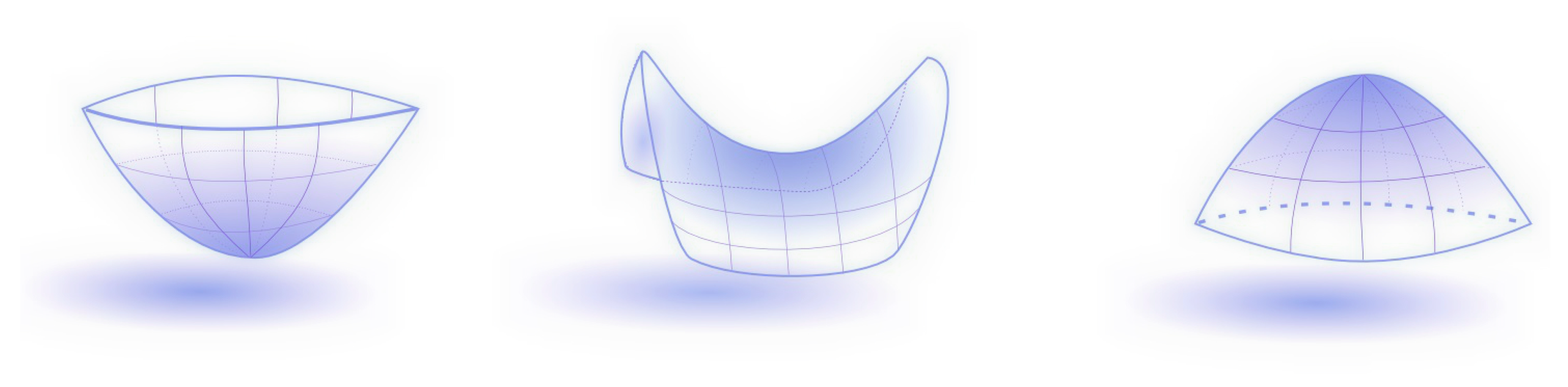
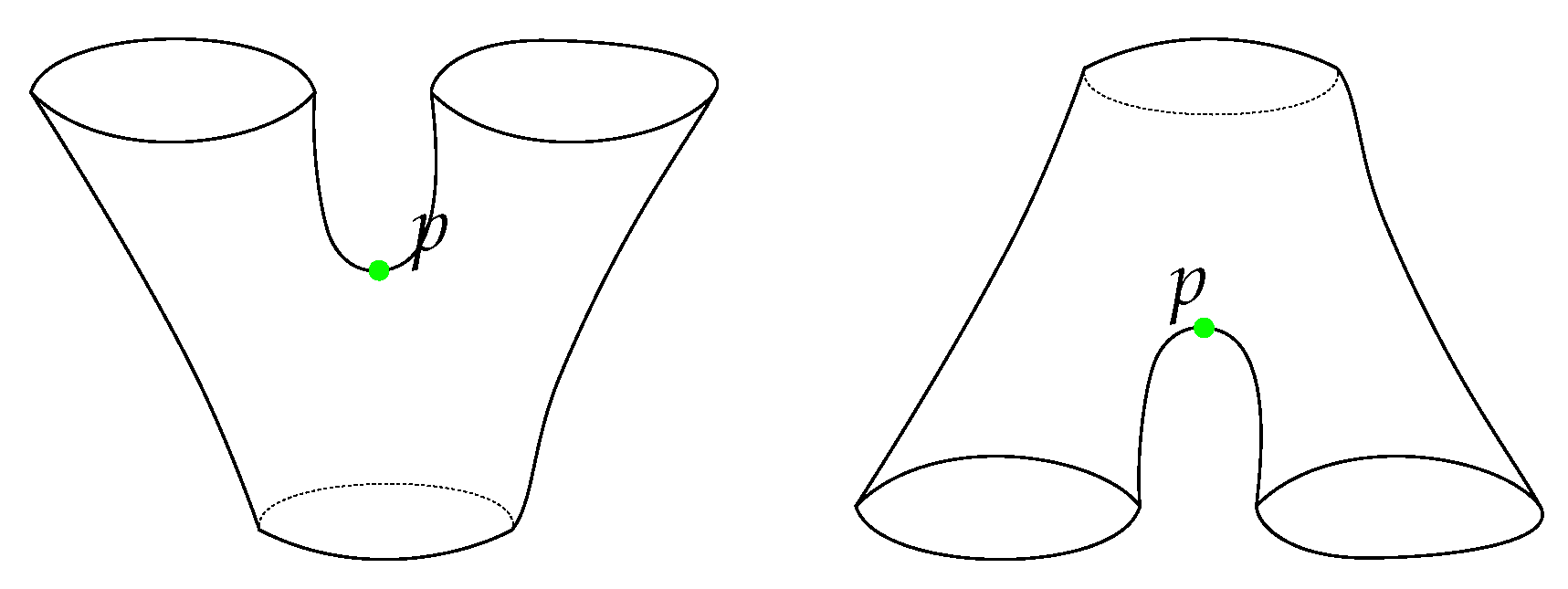
If f is a Morse function on a surface, then, up to a change of coordinates, the surface around a critical point f has one of the simple forms as appear in Figure 1. More formally, we have the following important Lemma:
Lemma 1.
(Morse Lemma) Let M be a smooth surface, be a smooth function, and p be a non-degenerate critical point of f. We can choose a chart around p, such that takes exactly one of the following three forms:
- 1.
- Local minimum—
- 2.
- Saddle—
- 3.
- Local maximum—
An analogous lemma holds for Morse functions on higher dimensional smooth manifolds. See [66] for more details. Morse Lemma implies that a Morse function around a critical point looks simple, and it is exactly one of the forms given in the Lemma above, up to a change of coordinates. Notice that the number of minus signs in the standard form of the function f around p is equal to the index of the critical point p.
2.2. Reeb Graphs
Let M be a topological space and let be a scalar function defined on M. The Reeb graph of the pair f and M gives a summary of the topological information encoded in by tracking changes occurring to the connected components of the level sets of f. More precisely, the Reeb graph of M and f is the quotient space of M defined, as follows. We say that the x and y are equivalent in M, and write , if and only if they belong to the same connected component of for some . The quotient space with the quotient space topology induced by the quotient map is called the Reeb graph of M and f. Here, recall that the map takes a point x in M to its equivalence class in . Given a point p in , it is often important in practice to retrieve the set of points in M that map to p via . In this article, we provide an efficient method to retrieve the data in M that are associated with a point on a Reeb graph.
The map induces a continuous function , where if . This map is well defined, since , whenever .
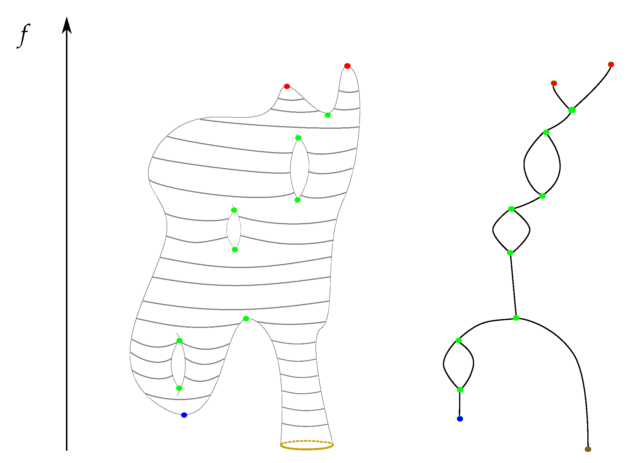
When M is a manifold and f is Morse, then exhibits certain additional properties. For instance, in this case, every vertex of arises from a critical point of f or a boundary component. Furthermore, every maximum or minimum of f gives rise to a degree 1-node of . Saddle points for a Morse function f defined on a 2-manifold have degree 3-node. This is not guaranteed if the scalar function is not Morse. See Figure 2 for an example of a Reeb graph.
3. Reeb Graphs on Triangulated Surfaces
3.1. Morse Functions in the Piece-Wise Linear Setting
In this paper, we will be working with triangulated surfaces. We will denote the set of vertices, edges, and faces of a triangulated mesh M by , , and , respectively. Banchoff provided the extension of Morse theory to triangulated manifolds [70]. Let M be a triangulated 2-manifold and let be a piece-wise linear function on M. We will use the abbreviation PL for “piece-wise linear”. The star of v, denoted by , is the set of simplices that intersect with the vertex v. The closure of is the smallest simplicial subcomplex of M that contains . The link consists of the subcomplex of M of simplices belonging to , but not to . The upper link of v is defined to be the set:
the lower link is defined similarly by:
and mixed link
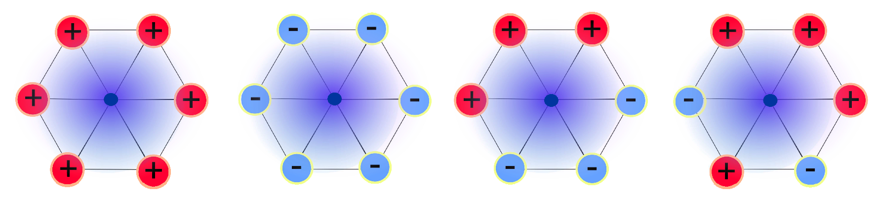
Using the link definitions, we classify vertices of M, as follows. A vertex v in M is PL regular if the cardinality of is equal to 2. If , then v is a PL maximum vertex with index 1, and if , then v is a PL minimum with index 0. If , then v is a PL saddle with index 1 and multiplicity . See Figure 3. A PL function is a PL Morse function if each vertex is either PL regular or PL simple, and the function values of the vertices are distinct. Similar to the smooth case, when , we further assume that f satisfies: (1) and (2) there are no critical points on .
3.2. Reeb Graphs of General Simplicial Complexes
Reeb graph can be defined naturally on arbitrary simplicial complexes. Let K be a simplicial complex and be a map defined on the vertices of K. The map f can be linearly extended to all simplices of K to PL function, which we will also denote denote by f. Using this function, the Reeb graph of can be defined as before.
4. Reeb Graph Sequential Algorithm on Triangulated Surfaces
In this section, we assume that we are given a PL function defined on a triangulated surface M possibly with a non-empty boundary . This includes the case when f is a Morse function. Subsequently, we discuss the degenerate case when f has non-simple saddles.
The algorithm above relies on Morse theory to find a finite set of paths traced concurrently inside parts of the manifold where the topology of the manifold with respect to a given scalar function does not change. The sequential algorithm that we present here is similar to the Reeb graph algorithm that is given in [26], where tracing paths inside cylinders were used to construct the Reeb graph. We provide the sequential version of the algorithm because it has some key differences from the algorithm given [26] that will be utilized later in our parallel algorithm.
The main idea of the algorithm is the construction of a sub-simplicial complex X of M, such that the Reeb graph of X with respect to , the restriction of f on X, is identical to the Reeb graph . The constructed simplicial complex X does not only provide us with a Reeb graph of , but also immediately implies an algorithm to compute the map that allows for us to extract the manifold data given the corresponding Reeb graph points. The main two ingredients of the algorithm are the critical sets and the ascending paths. We introduce these two concepts next.
4.1. Critical Sets and Ascending Paths
We start by giving the definition of critical sets. Subsequently, we provide the definition of ascending paths.
Critical Sets.
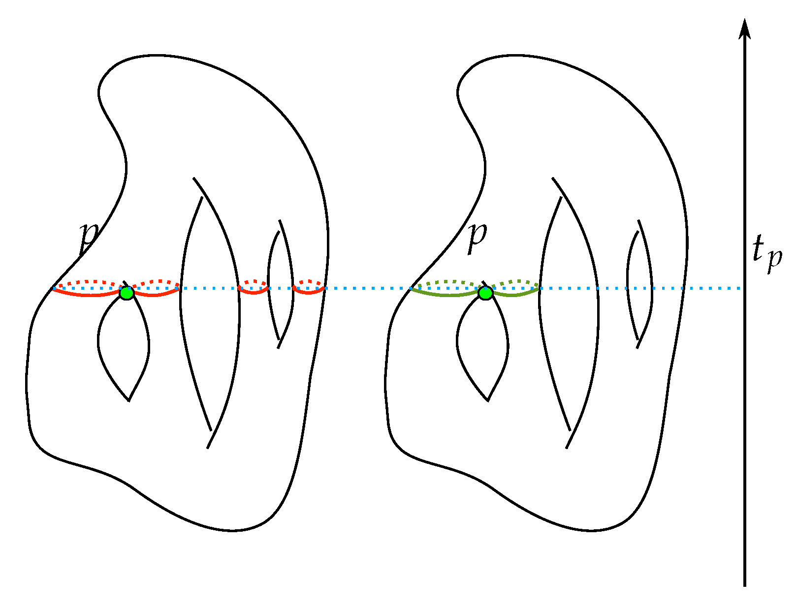
Let p be a saddle point of f, and let be its corresponding critical value. Consider the connected components of the set . The connected components of consist of a collection of simple closed curves embedded in M, as well as a single component, which contains a singularity. This singular set consists of multiple circles that intersect at the critical point p. We will denote this singular set by . See Figure 4 for an example. Note that, for critical value t might merely consist of the critical set (with no other simple closed curves).
Choose small enough, such that the interval has only the critical value . As we move from to , the singular set becomes a non-singular one consisting of a disjoint union of simple closed curves , for . By convention, we will consider the sets to be the connected components of the singular set , and we will refer to them as such for the rest of the paper. We talk more about the components of a critical set and show exactly how to determine them in the piece-wise linear setting in Section 4.2.1. The following Lemma asserts that the number of connected components of of for a simple saddle point of a Morse function defined on the surface is either 1 or 2.
Lemma 2.
Let M be a compact connected orientable surface with more than one boundary component. Let be a Morse function on M such that . If f has a unique saddle point, then M is homeomorphic to a pair of pants. See Figure 5.
For a regular value t, we will denote the number of simple closed curves of by . Lemma 2 implies that, for a sufficiently small enough and for any saddle point p on a Morse function f, one has . In other words, as we are passing through a saddle point p, two circles merge or split. Figure 5 shows two types of saddles: a split saddle and a merge saddle. A saddle point p is a split saddle if , and it is a merge saddle if .
The sequential version of the algorithm relies on Lemma 2 to handle the case when the function f is Morse and it only has simple saddle points. The case when f has saddle points with higher multiplicities will be handled in Section 4.5.
Remark 1.
If p is a maximum or minimum point, then by definition, will be the set that consists of the point p itself.
Ascending Paths.
The second main ingredient of the sequential Reeb graph algorithm is a collection of curves that we trace inside the manifold M using the function values. More precisely, an ascending path from a non-maximum vertex , denoted by , is defined to be a finite sequence of consecutive edges on M, such that is an edge on M for , , and is a maximum, a boundary or a saddle vertex.
4.2. Outline of the Sequential Algorithm
Now, we present the outline of the sequential Reeb graph algorithm. We assume that we are given a triangulated PL Morse function defined on triangulated mesh M without boundary. The case when the function f is not Morse, or when the M has a boundary, will be discussed in later sections.
The sequential Reeb graph algorithm is given in the following steps:
- We start by sorting the critical points of f by their critical values. Let be the set of the sorted critical points of f in an ascending order.
- For each critical point of the function f, we define a node in the Reeb graph . In other words, the node set of the graph precisely corresponds to the set of critical points of the function f defined on M.
- For each critical point v in , we compute the critical set .
- For each saddle or a minimum vertex v in , we associate one or two ascending paths on the mesh: one ascending path if v is a minimum or a merge saddle, and two paths if v is a split saddle. For each ascending path, we march with until this path intersects with the first critical set with a higher critical value than of . At this point, we insert an edge for the Reeb graph between the vertex v and vertex w.
Figure 6 illustrates the steps of the algorithm. It remains to describe two aspects of the previous algorithm: the construction of the critical sets mentioned in step (3) and the construction of the ascending paths that are mentioned in step (4).
4.2.1. Construction of the Critical Sets
We now describe how to compute the critical set of a critical point in the piece-wise setting. As before, we assume that a piece-wise linear function is defined on a triangulated surface M, and it takes distinct values on the vertices of M. This assumption will guarantee that, for a given value t, the level curve intersects with, at most, one vertex of M.
Now, let . The cross simplices of the value t is the union of all simplices of M, which intersect with the level curve . This is the set of vertices, edges, and faces in M, which intersect with the level curve . We define to be the closure of the smallest subcomplex of M, which contains . If for a vertex v in , then we define the subcomplex as above, but we also add to it the simplices of .
When t is the maximal or the minimal value, then consists of a single vertex . In this case, is simply . When t is a regular value, then is a disjoint union of topological cylinders, that is, appears as a “thickened” band around the curve Note that, when the value t that corresponds to a vertex v in with for some v in M, then the set of simplices in the intersection is simply the vertex . When t is the critical value of a saddle point, then the curve consists of a finite collection of simple close curves that meet at the saddle point, and the set can be seen as the thickened band of these curves. See Figure 7.
The ower level of the cross subsimplex of a value t, denoted by , is the set of vertices and edges in , which have values less than or equal to t. Similarly, the higher level of the cross subsimplex of a value t, denoted by , is the set of vertices and edges in , which have values higher than or equal to t. See Figure 7.
Recall the notion of the connected component of a critical set from Section 4.1. Specifically, for a critical vertex v with a critical value , we talked about the connected components of the critical set . Using the definitions that are introduced in this section, we can compute the connected components of the critical set in the piece-wise linear setting by considering the connected components of .
4.2.2. Construction of the Ascending Paths
The ascending paths from a critical point are specified, as follows:
- If is a merge saddle or a minimum, then we initiate a single ascending path specified, as follows. Let be a vertex in such that . At the kth iteration, consists of with for .
- If is a split saddle, then we start two ascending paths and originating from the point p specified as follows. Divide the set into two disconnected components A and B. Choose the vertex in A, such that for all , and choose the vertex in a similar manner. At the kth iteration, consists of with for (here we assume ). The path is similarly constructed.
4.2.3. Termination of an Ascending Path
The condition at which we terminate the ascending paths we initiated in step is specified as follows. Assume that we initiated an ascending path from a critical vertex v. Let w be the critical vertex with the critical value right after the critical value of v. Assume that, at the kth iteration, an ascending path starting from the vertex v is . We continue this iteration until we arrive at an edge with and . At this point, we check the condition . If this condition is satisfied, then we insert an edge for the Reeb graph between the vertex v and the vertex w. If , then we keep marching until an edge in the ascending path meets a critical point w that satisfy these two conditions. Note that w can be either a saddle or maximum vertex.
The check of intersection between the edge in an ascending path and a critical set , as mentioned in step (4), can be done by checking if belongs with .
Remark 2.
It is important to notice how an ascending path corresponds to an edge in the Reeb graph. The ascending path starts at a critical point p with a critical value and terminates at a critical set that corresponds to a critical point q with a critical value with . More precisely, an ascending path starts at one of the connected components of the upper link of a critical point p and ends at one of the connected components of the critical sets . If two ascending paths start at two different connected components of the upper link of p, but still end up in the same connected component of , then these two paths correspond to the exact same edge in the Reeb graph. Therefore, only one of these ascending paths corresponds to an edge in the final Reeb graph. For this reason, we say that each ascending path starting from a connected component of the upper star of a vertex gives rise to a potential edge in the Reeb graph. We provide more details on this point in Section 4.5.
4.3. Surfaces with Boundaries
In the case when the surface M has a boundary, we modify the previous algorithm, as follows. In this case, is not empty and consists of a finite collection of simply closed curves. We treat each connected component of as a minimal point, and we treat the boundary as a maximum point. More precisely, the following modifications are added to the previous algorithm from Section 4.2.
- In step , each connected component in is considered a vertex in the Reeb graph vertex set.
- In step , for each boundary component in , we pick an arbitrary vertex on the boundary and initiate an ascending path that starts from that vertex.
- In step , if an ascending path starting at a vertex v reaches a boundary vertex w in one of the connected components, say , of , then we insert an edge in the Reeb graph between the vertex v and vertex in that corresponds to .
We denote the subcomplex obtained from M using the previous algorithm by . In other words, consists of the critical sets for all critical points p, as well as the ascending paths we initiated at the saddle, minimum, or boundary vertices. When M and f are clear from the context, we will denote simply by X.
4.4. Correctness of the Sequential Algorithm
For a function and define:
Note that we allow to be empty. Moreover, we define:
The correctness of our algorithm relies on the following two facts:
- The only topological changes to the level sets of f occur when as pass a critical point. This is formally stated in Theorem 1.
- The structure of the manifold around a critical point is completely determined by the index of that critical point. We give this in Theorem 2.
The proof of Theorems 1 and 2 can be found in [69].
Theorem 1.
Let be a smooth function on a smooth surface M. For two reals with , if f has no critical values in the interval , then the surfaces and are homeomorphic.
The above algorithm relies on Theorem 1. Namely, as we trace an ascending path, we assume that no topological change occurs until we reach the next critical point. The ascending path may not terminate at the next critical point, provided the part of the manifold in which this path is traveling in has not changed its topology. This will become more evident after we provide the next theorem, which shows the exact structure of around a critical point.
Theorem 2.
Let M be a compact connected surface, possibly with a boundary, and let be a Morse function on M. Let p be a critical point and let t be its corresponding critical value. Let be small enough, so that has only the critical value t.
- 1.
- If is equal to 0 or 2, then is homeomorphic to a disjoint union of a disk and a finite number of topological cylinders (that is a genus zero surface with two boundary components).
- 2.
- If , then is homeomorphic to a pair of pants and a finite number of topological cylinders.
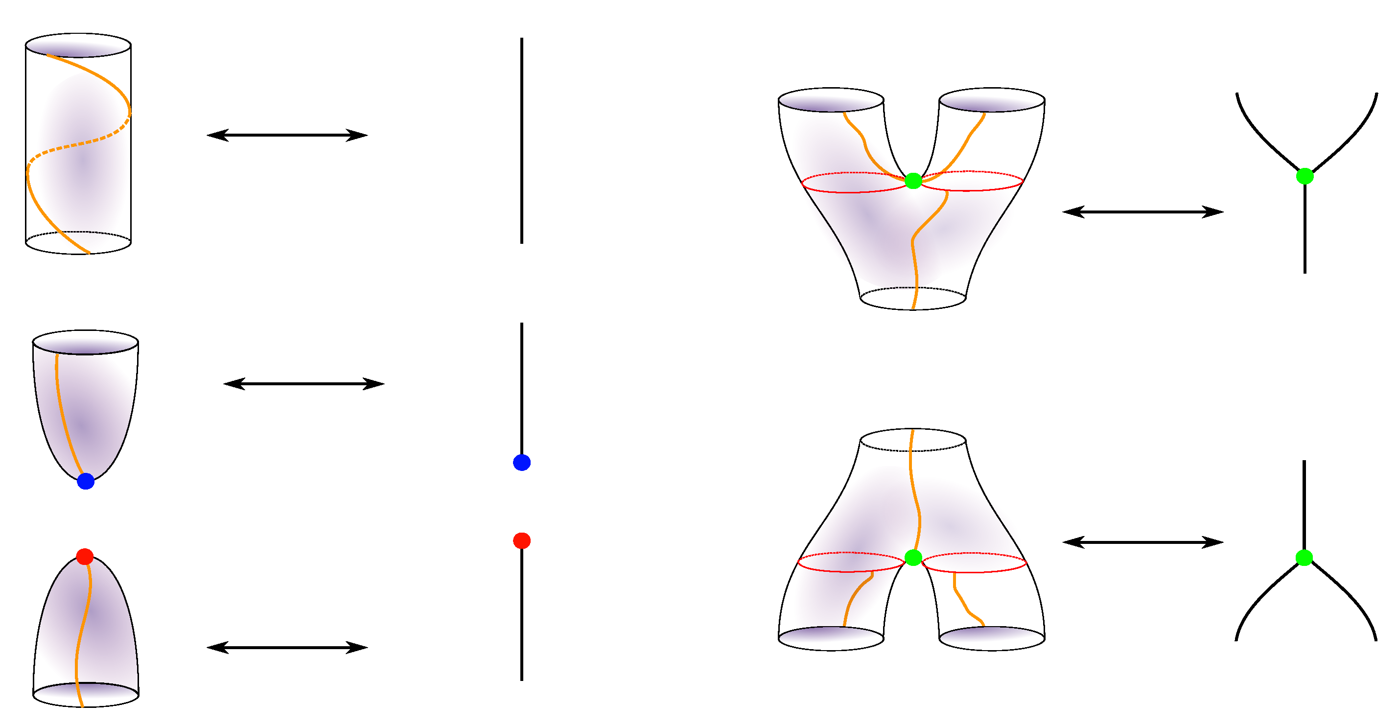
The previous two theorems show that for a given Morse f function on M, we can arrange M so that at each critical point, only a single topological event occurs, and this topological event occurs around the critical point. Moreover, we know exactly what topological event occurs by considering the index of the critical point. Figure 8 illustrates this.
Moreover, subcomplex constructed in the algorithm has the same Reeb graph structure of that of M around the critical points. See Figure 10.
This shows that any two-manifold can be built from the building blocks in Figure 9. Moreover, Theorem 2 shows that the restriction of f on has the shapes that are given in Figure 10. In other words, this gives us the structure of the Reeb graph around an interval that contains a single critical value.
Now, let be an edge in a Reeb graph connecting between the two nodes p and q, which correspond to critical points of f. For each such edge, we can find a preimage arc E in M that is mapped to via the map . The preimages of the value p and q under are the critical set and in M, respectively. Hence, each arc E must start at a point A in and end at a point in B in . Each arc on M characterizes the edge e.
An ascending path that is constructed in the sequential algorithm essentially traces an arc in the way described above. Namely, for a critical point p, with a critical value , an ascending path created at a point p will terminate at a critical point q with . This termination occurs when we pass through the critical set of the point q.
4.5. Dealing with Degenerate Cases
It is possible in practice to obtain a scalar function with saddle points that have multiplicity . The algorithm that we present in Section 4.2 can be extended to handle such cases. We need to make the following modifications.
- In step (3), we calculate the connected components of the critical set . Here, it is not enough to calculate the critical set . We also need to compute the connected components of this set. Section 4.2.1 explains this.
- We create an ascending path for each connected component in when the multiplicity m of a split saddle p is greater than or equal to 2.
In the non-degenerate case, every ascending path corresponds to an edge in the Reeb graph. This is not the case anymore in the degenerate case. Nect, we describe the sequential algorithm of the Reeb graph when f has degenerate critical points.
- Sort the critical points of f an in ascending order. Let be this set. This represents the vertex set of the Reeb graph, as we did before.
- For each v in , compute the connected components of and include all of these components in a single container . We will denote, by , the connected component j of the critical set . In this way, we index all of the elements in .
- Declare each set of as not visited.
- For each critical point in and for each component in , we initiate an ascending path P as described in Section 4.2.2. For each such path, we determine the connected component in , which the path terminates, as described in Section 4.2.1. We have two cases:
- (a)
- If the connected component is not visited, then we insert an edge between and and mark the component as visited.
- (b)
- If the connected component is visited, then we do not make any changes to the Reeb graph and terminate the current ascending path. In this case, the ascending path corresponds to an edge that already exists in the Reeb graph. See Remark 2.
Note that the above procedure can be used to determine the edges that originate from a simple saddle. Namely, we do not need to check the type of the simple saddle point (merge or split) in step (3) of the algorithm given in Section 4.2, and for any saddle point, we use the above procedure instead.
5. Parallelization of the Algorithm
In this section, we give the details of our strategy to compute the Reeb graph in parallel. We describe the three stages of the parallel algorithm as follows.
- The Partition Stage. In this stage, we partition the manifold M into submanifolds, such that the vertices counts of each submanifold are approximately equal to each other.
- Computing the Reeb Graph for the Submanifold Stage. Computing the Reeb graphs for each submanifold obtained from stage one concurrently.
- The Gluing Stage. In this step, we glue the Reeb graphs that were obtained from stage 2.
5.1. The Partition Stage
In this first stage of the parallel algorithm, we sort the vertices of the manifold with respect to the function f. This step can be done efficiently in parallel [77,78]. The critical sets for saddle points are then determined by assigning a thread to each saddle point. This computation is only necessary to determine the number of ascending paths that we need to initiate from that saddle point. Next, we partition the manifold M to submanifolds along with certain regular values of the scalar function f. More precisely, the partition stage is given, as follows:
- Compute the critical points of f by assigning a thread to each vertex in M. Let be the list of critical points of f, and let be their corresponding critical values.
- We choose k regular values of f. These values will be utilized to slice the manifold M into submanifolds , such that the vertex counts of the submanifolds are approximately equal to each other. We also need to determine the connected components for in C. The connected components of the regular value can be computed in linear time with respect to the number of edges in M, as follows. We visit all edges of M and detect if an edge crosses one of the values . If such an edge is found at a level , then we keep rotating around to find all other edges crossing the value within the same connected component of . After visiting all edges, we have also determined the connected components of for each . We will denote the set of all connected components of for by . We also call an edge in M that crosses a crossing edge. See Figure 11 for an illustration.
- Divide the surface M into partitions along the level sets for all . We obtain a list of submanifolds ,…,. Here, we set and . We will denote to by . The set will be denoted by .
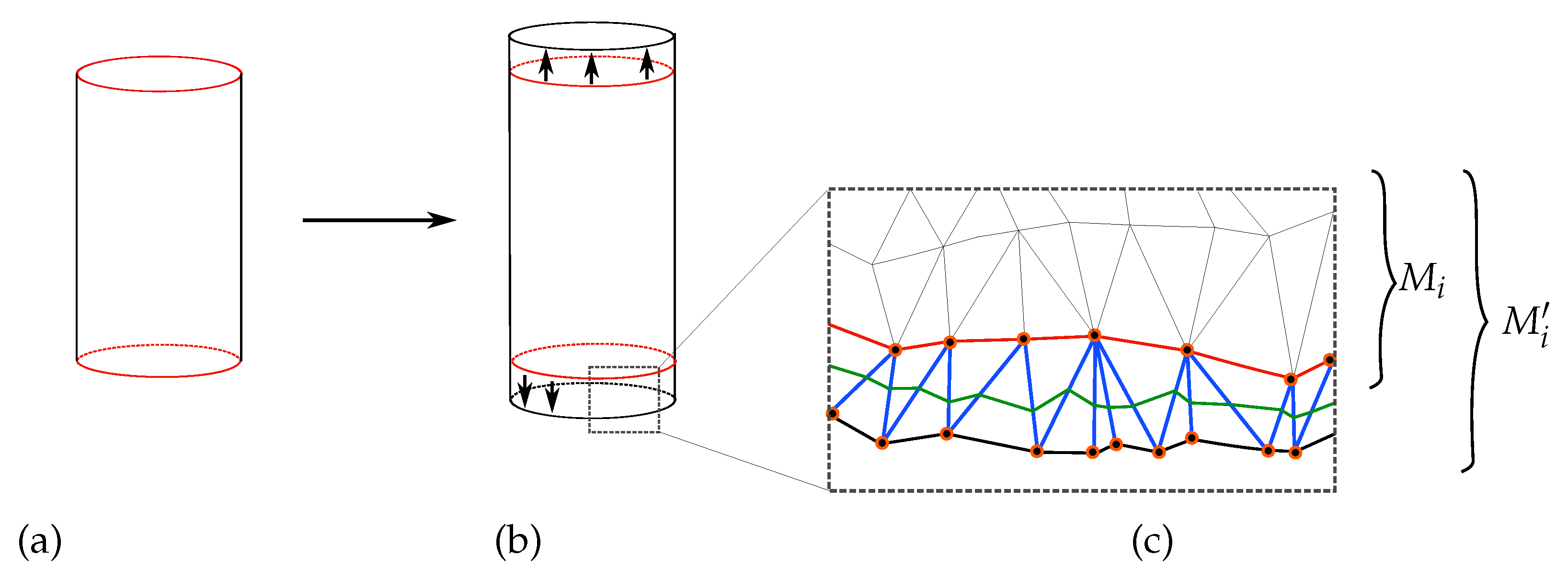
- Next, we extend by adding other vertices in M as follows. Let and be the edges in M that intersect with and , respectively. The submanifold is obtained from by adding the vertices from and . We call the edges and the boundary edges of . Note that every two consecutive submanifolds from intersect with each other along their boundary edges. See Figure 12 for an illustration.
The purpose of extending the submanifolds to in step (3) will be justified in the gluing stage in Section 5.3.
5.2. Computing the Reeb Graph of Each Submanifold
The manifold is, in general, homeomorphic to the manifold , since the former is obtained from the latter by slightly extending its boundary. However, in the piece-wise linear case, the extension specified in the previous section may change the topology of the manifold. This will occur when a crossing edge in or contains a critical vertex of f. When this case occurs, we exclude this vertex from in order to keep it homeomorphic to . Using this convention, we can assume that the Reeb graph of the restriction of f on is identical to the Reeb graph of the restriction of the Reeb graph of f on .
Computing the Reeb graphs for , for , now goes, as follows. To each connected component in for , we assign a thread and the Reeb graph on the submanifold , which can be concurrently computed.
An ascending path that starts at a crossing edge or ends at a crossing edge will be treated specially. We call the Reeb graph edge that corresponds to such an ascending path a crossing arc. Furthermore, if the starting or the ending edge of this ascending path is a crossing edge, then we will call the corresponding node in the Reeb graph a crossing node. Every crossing node is determined by its crossing edge. In other words, given a crossing edge, we can recover its crossing node in the graphs for . In practice, we need to be able to do this in constant time, so we create a global map G that takes as an input a crossing edge and returns its corresponding crossing node. In the case when a single crossing edge is associated with two crossing nodes from two consecutive submanifolds, then the map G associates that edge crossing edge to the two crossing nodes (this occur when the ending edge of a crossing arc and the starting edge of the crossing arc in the consequent submanifold are the same). If the crossing edge is not associated with any crossing node, then this map returns a constant value indicating that this edge is not a starting or an ending crossing edge for any ascending path. Note that each connected component in has either two crossing edges that are associated with two crossing nodes or a single crossing edge that is associated with two crossing nodes. This map will be utilized in the gluing stage.
5.3. The Gluing Stage
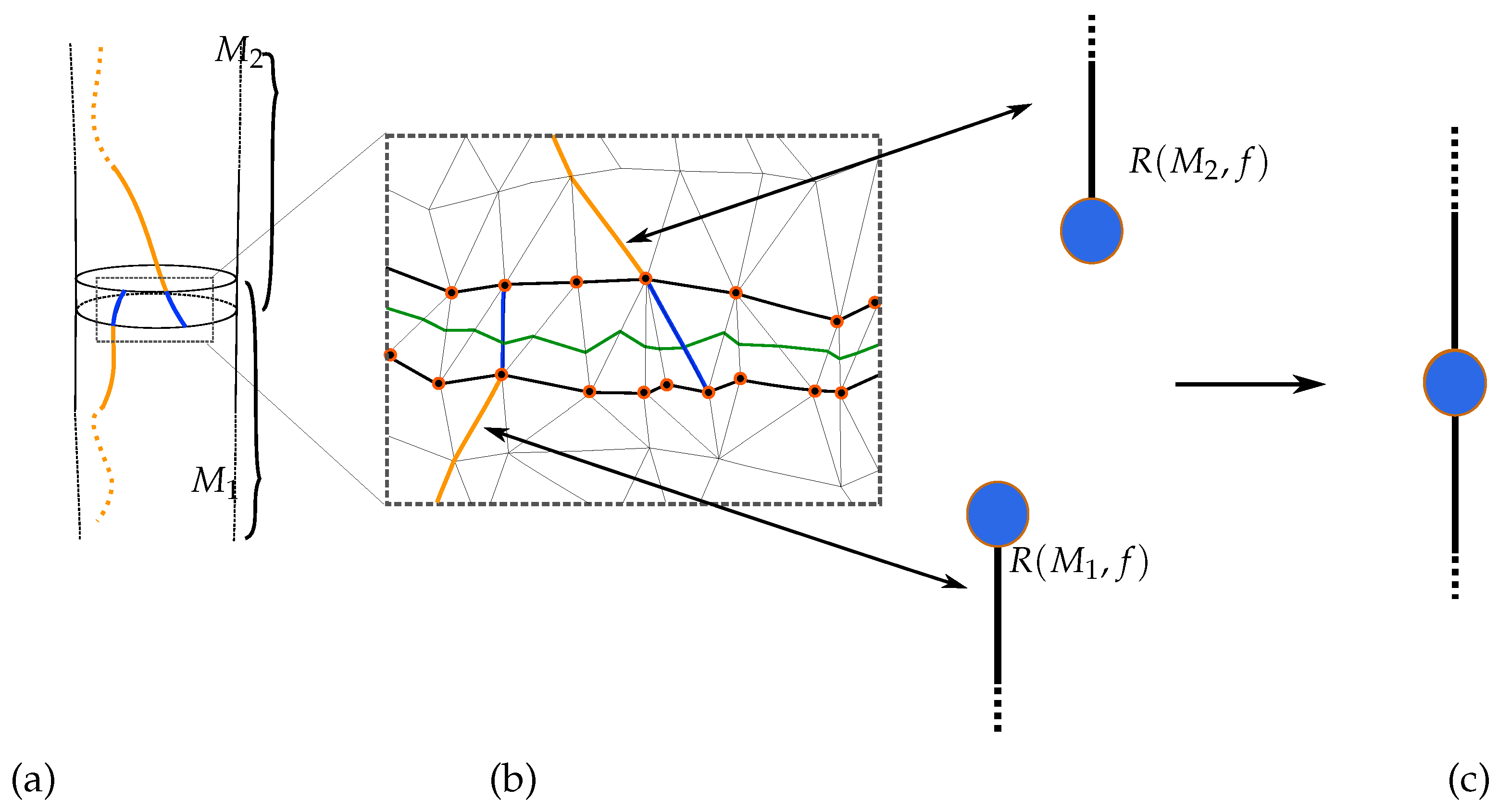
For the gluing stage, we need to glue the nodes of the Reeb graphs that occur in duplication . For this purpose, we utilize the function G that we constructed in Section 5.2. For each connected component in , we visit its crossing edges and check whether two edges within that connected component have been flagged by G. If this is the case, then we retrieve the crossing nodes that correspond to these two edges via the function G and glue them. In the case when a connected component of has a single crossing edge, then we retrieve the two crossing nodes that are associated with that edge and glue them. When we finish visiting all connected components of , all duplicate nodes will have been glued, and the final graph is . See Figure 12 for an illustration of this process.
6. Augmented Reeb Graph Computations: Going from the Reeb Graph to the Manifold
In this section, we give an algorithm that describes an explicit computation of the map . The computation of this map, alongside the computation of the Reeb graph, is usually called the augmented Reeb graph [17]. Our algorithm here is the first parallel augmented Reeb graph algorithm that we are aware of. This map associates every vertex v in the graph to the critical set associated to that critical point. More importantly, for each interior point p of an edge in , we want to associate a simple closed curve in M, such that .
6.1. Building the Augmentation Map
In the construction above, for our Reeb graph algorithm, an edge of the graph is traced as a sequence of edges on the mesh running between two critical sets of the function f. This immediately gives an embedding of the edges of the Reeb graph on the surface. This embedding is used to get the circle corresponding to any points on the graph. More precisely, we have the following correspondence. Let e be an edge of the graph . By the construction of our algorithm, every edge in is determined by two critical points and a sequence of oriented edges on the mesh. Let be the sequence of oriented edges on the mesh M that corresponds to the edge e. If , then we will denote by to . Let be the summation , where .
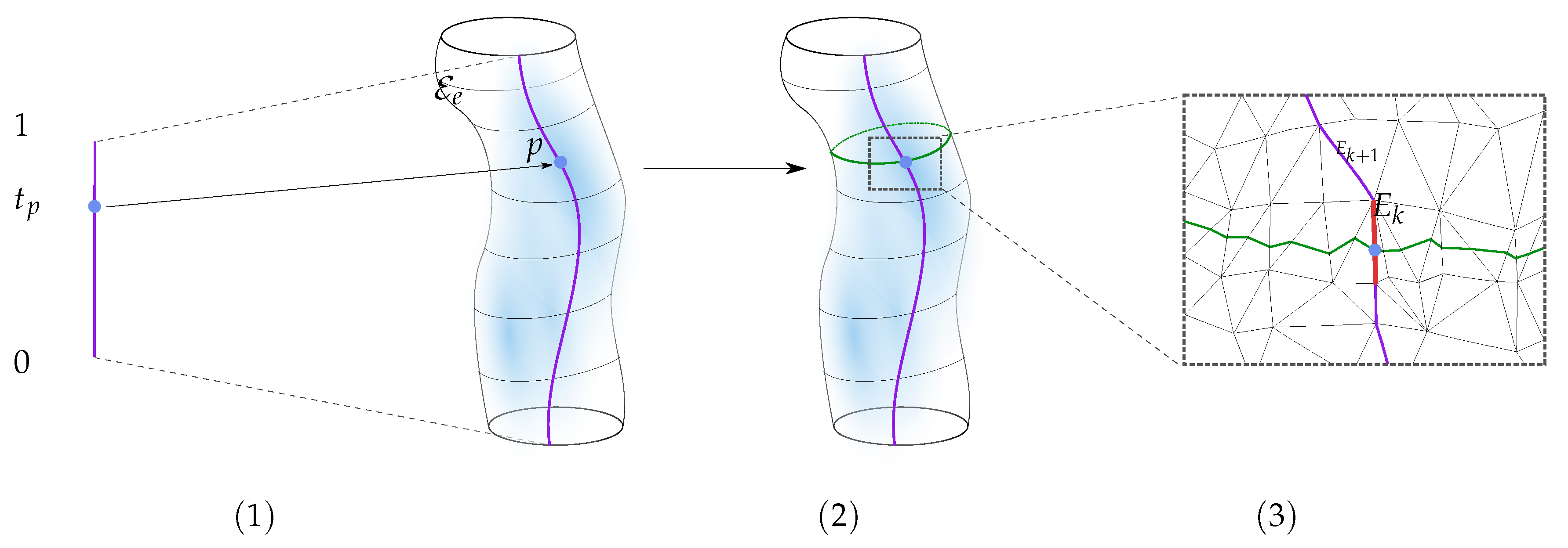
An interior point p, on the edge e, is specified by giving a value in the interval . We do the following procedure to obtain the circle on the mesh M that correspond to p:
- Map the interval linearly to the interval .
- Use the constructed linear function that is computed in step (1) to map to its corresponding value in .
- Determine the edge in , such that .
- Now, we need to find the value t, in the range of , the range of f, such that contains . We know that this value corresponds to , which lies in the interval . The required t lies in interval . Hence, we map the interval linearly to and determine the value t in that corresponds to .
- The required circle is precisely the connected component of that contains the edge .
See Figure 13 for an illustration of the main parts of the previous procedure.
Note that, in the previous procedure, we rely on the fundamental assumption that f takes different values on the vertices of the mesh.
6.2. Consistent Parameterization of the Edges of the Reeb Graph
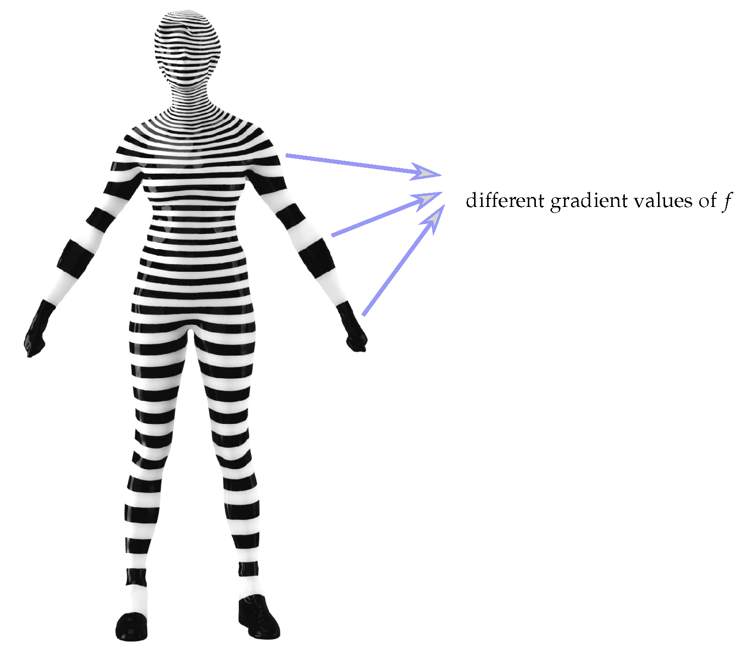
Going back to Section 6.1 we observe that the mapping between and depends on the gradient of the function f. More specifically, recall that . Hence the values of for a given edge E can be interpreted as the gradient of f along that edge. Hence, the derivative of the function in not constant in general. This variability in the derivative can make it difficult and less intuitive to choose a value t in that corresponds to a specific curve on the mesh, because, while the mapping between is linear, the function is not linear in general. See Figure 14 for an illustration of the gradient problem.
To this end for a given function f, we want to construct another function that has the following two properties:
- The levels sets of the function are parallel the level sets of f.
- The function has uniform gradient everywhere.
We need to recall the definitions of gradient and divergence of a triangulated mesh quickly before we give the construction of .
6.2.1. Gradient and Divergence of a PL Function on a Triangulated Mesh
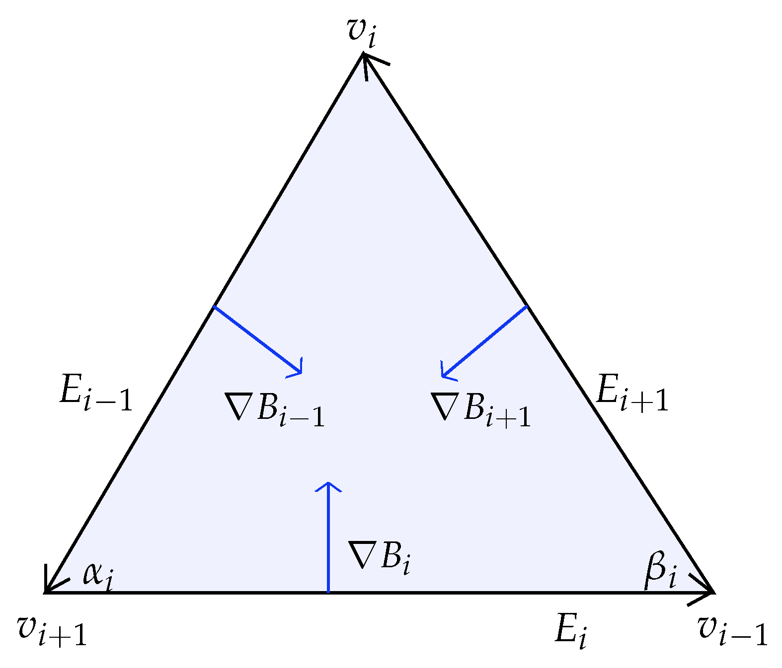
Let f be a PL scalar function on a triangulated manifold M. Let be a face in M. Denote by the counterclockwise oriented edge opposite to the vertex . See Figure 15. Let be the hat function on the vertex defined by for . The gradient of f is a constant and tangential vector on given by [79]:
where
Here, is a unit vector perpendicular to the vector and oriented so that it points into the face and is the area of the face . See Figure 15.
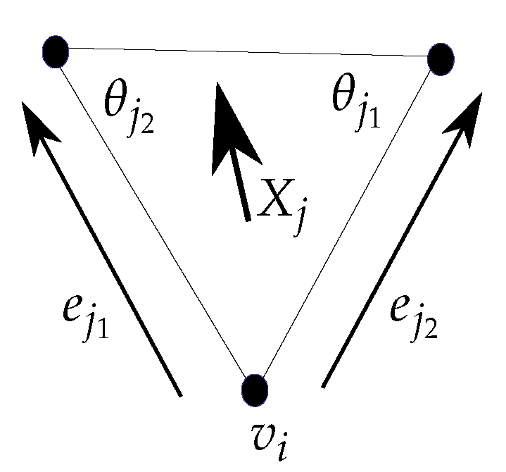
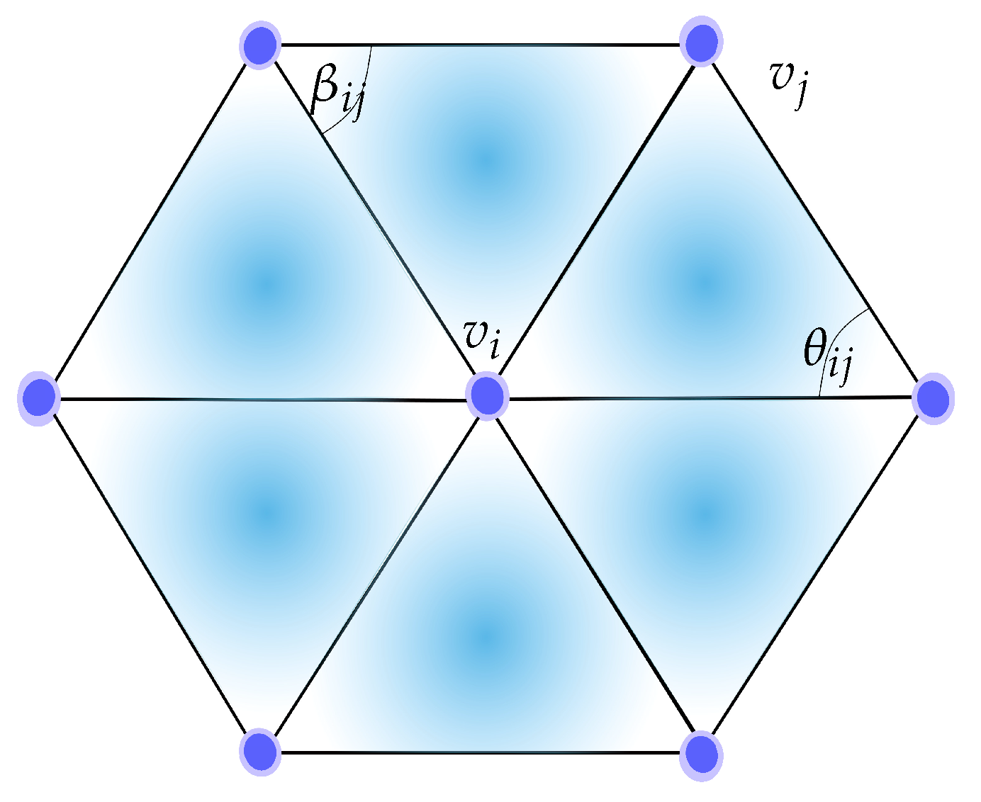
The divergence of a vector field X defined on the vertices on M was given in [80] and it can be computed via the formula:
where is the set of indices of all faces that are incident to the vertex , are the two vectors in face j that contain the vertex and are the angles that are opposite the edges and , respectively. See Figure 16.
6.2.2. Unit Gradient Scalar Fields
Now, given a function on a triangulated mesh M, we are interested in finding a function with the following two properties:
- The levels sets of the function are parallel to the level sets of f.
- The function has uniform gradient everywhere.
The above two conditions are equivalent to constructing a function such that . Setting finding such can be obtained by solving the following Poisson equation:
which is equivalent to solving , where is the Laplacian of the mesh M. Hence, finding the function can be reduced to the following two simple steps:
- Compute
- Solve the Poisson equation .
The previous algorithm works on any generic function f, such that the gradient of f is not zero. Moreover, Step (2) can be easily solved while using the definitions of the gradient and the divergence provided earlier. The above simple procedure is a generalization of the geodesic in heat method [81], where the desired function represents a distance function.
Figure 17 illustrates an example of such a procedure. The right model in the figure shows a solution for a scalar function obtained as a Poisson equation where X is the normalized gradient of the original function f shown on the left. Observe that the level sets of both f and are parallel, but now the gradient of is constant.
7. Run-Time Analysis and Implementation
We tested the presented algorithm on meshes with various complexities. In particular, we performed the speedup analysis of the parallel algorithm to our implementation of the sequential version given [26]. Our experiments were done on an AMD FX 6300 6-Core with 32 GB memory. The algorithm was implemented in C++, and the Windows platform was used.
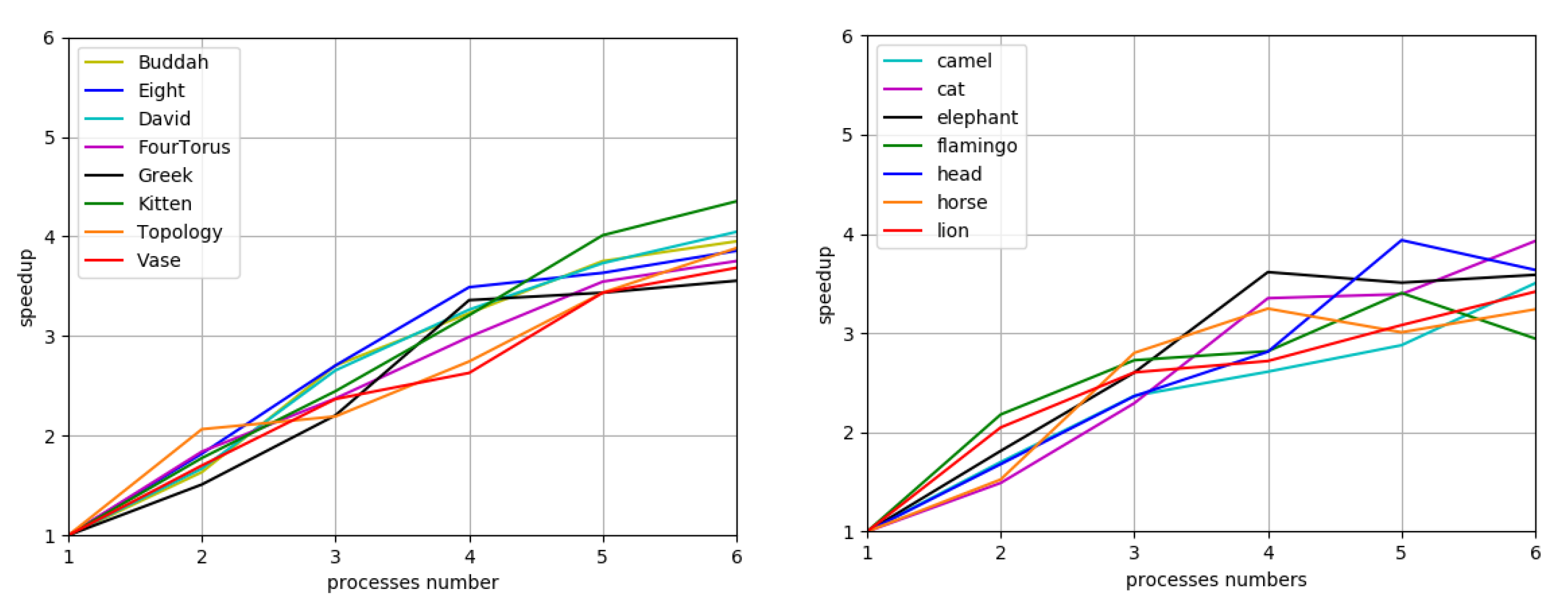
We test our parallel algorithm with two datasets: the AIM@SHAPE Repository as well as the MeshDeform dataset available in [82]. The initial attempt did not give us an increase of performance over the sequential algorithm for most of the meshes available in the above datasets. We tested our algorithm on high resolution meshes in order to take advantage of the parallel implementation. Specifically, we uniformly increase the resolution of the meshes available these two datasets to 200 k. On the AIM@SHAPE library our implementation gave us a minimum speedup of 3.6, a maximum one of 4.3, and an average speedup of 3.8 on six cores. Using this, we obtain a average parallel efficiency. One the MeshDeform dataset we obtained a minimum speedup of 2.9, a maximum one of 3.9, and an average speedup of 3.5 on siz cores. This dataset gives a average parallel efficiency on six cores. Figure 18 provides the details. The x-axis represents the number of processes, and the y-axis shows the speedup.
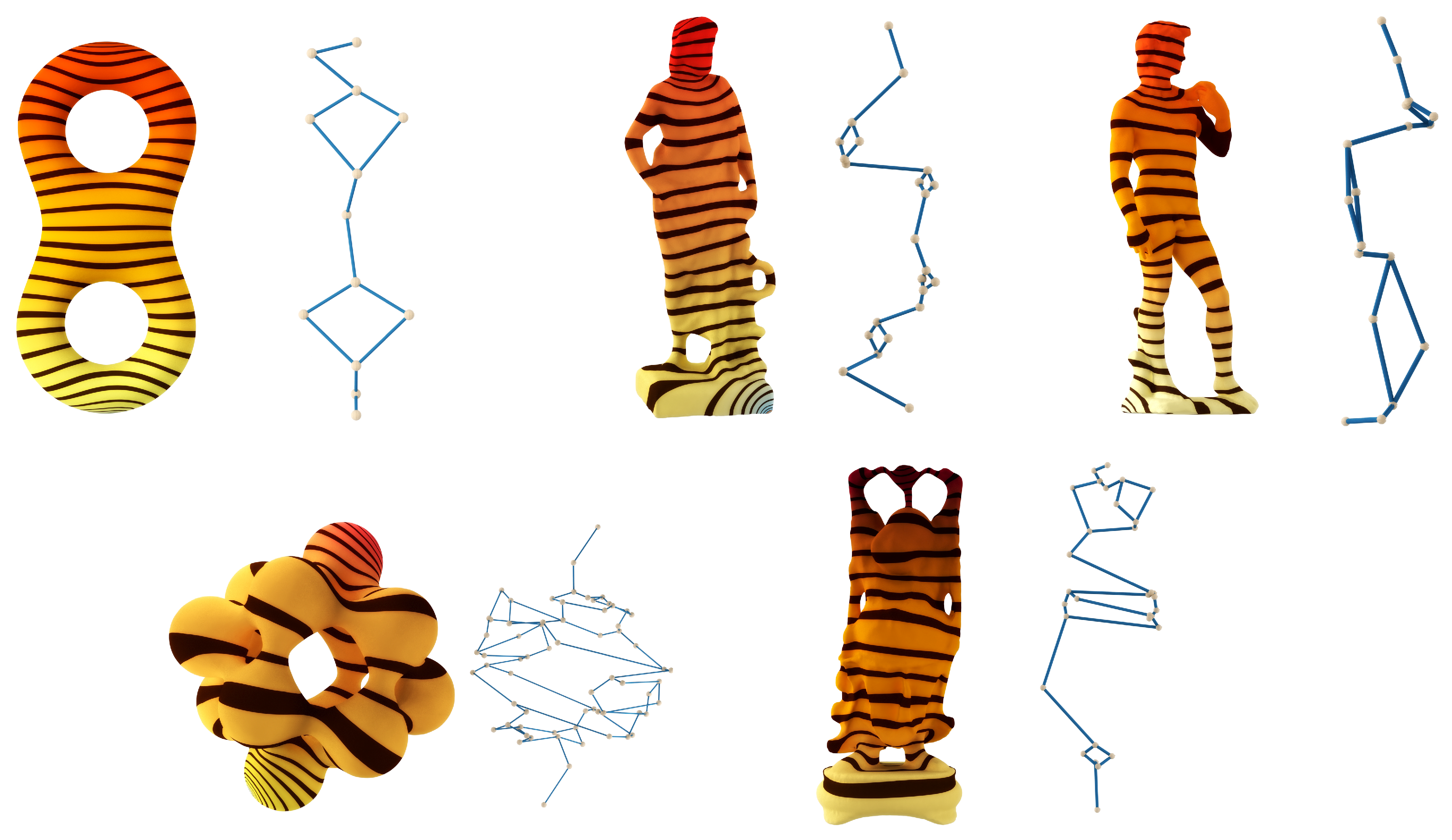
Figure 19 shows a few examples of the meshes that we utilized in our tests above, along with their corresponding Reeb graphs.
8. Applications
Reeb graphs on a surface M encode a rich amount of topological information from the original surface. In this section, we show how the Reeb graph of a surface M gives rise to a natural collection of simple closed curves on M. The applications that we present can be described in terms of these curves. We first define these curves and show their relation with the Reeb graph. We then give a procedure to extract them by utilizing the tools that we described in Section 6. Finally, the curves are utilized to obtain two higher genus surface mesh segmentation algorithms. Other Reeb graph-based segmentation algorithms can be found in [54,83,84].
Let be a surface M and a scalar function f. The edges of the Reeb graph determine the following types of simple closed curves on M:
- Cutting system curves.
- Pants decomposition curves.
- Branch curves.
We describe how a Reeb graph on a surface can be used for realizing these curves next.
Cutting System Curves.
Reeb graphs can also be used to determine the so-called cutting system. A cutting system for a connected, closed, orientable surface M of genus g is a collection of unordered disjoint simple closed loops embedded in M whose complement is a sphere with 2 g boundary components [85]. Segmenting a surface along a cutting system curve yields a genus zero surface with multiple boundary components. Hence, this can be used to aid in mesh parametrization. See, for instance, [86] and the references therein. Here, we describe a Reeb graph-based algorithm to obtain a cutting system. The algorithm is illustrated in the Figure 20 and it goes, as follows:
- Let T be a spanning tree of and consider the edges in .
- Select an interior point in , for .
- Each interior point selected in the previous step determines a loop , which can be obtained using the Reeb graph algorithm we described here.
The steps of the cutting system algorithm are described in Figure 20.
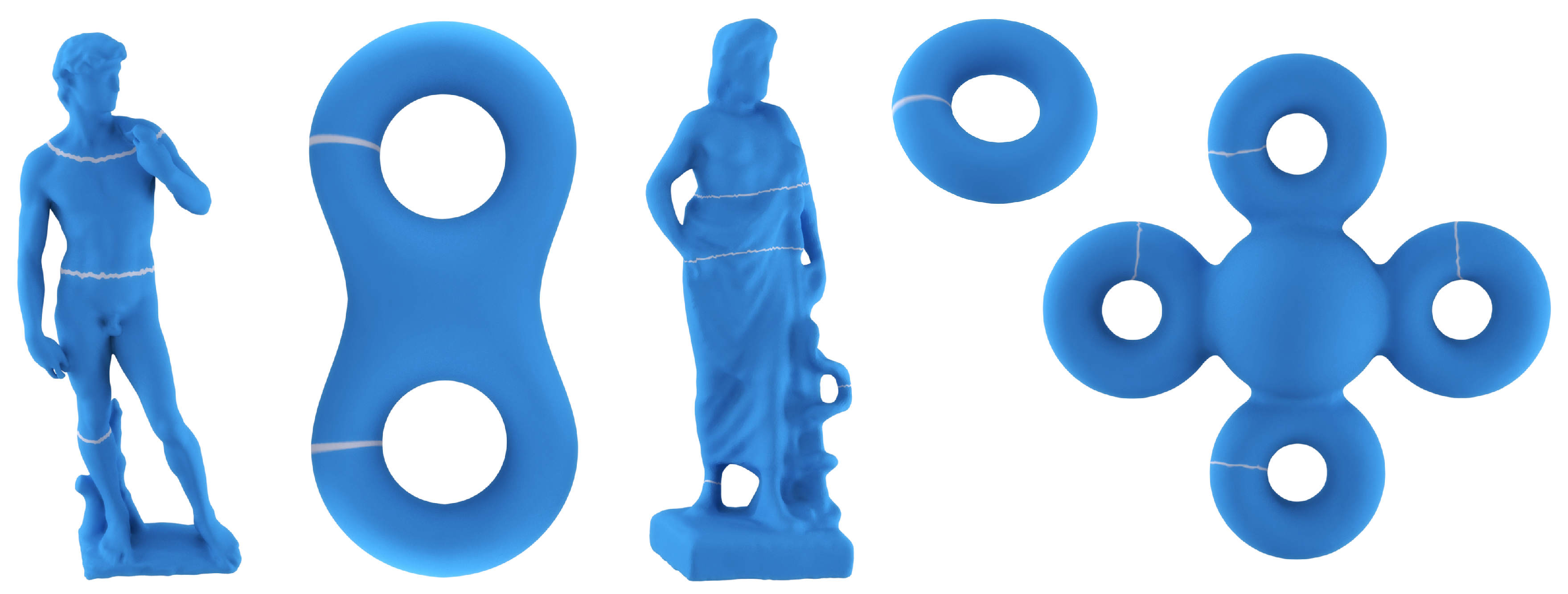
Figure 21 shows multiple examples of cutting system curves on triangulated surfaces.
Pants Decomposition Curves.
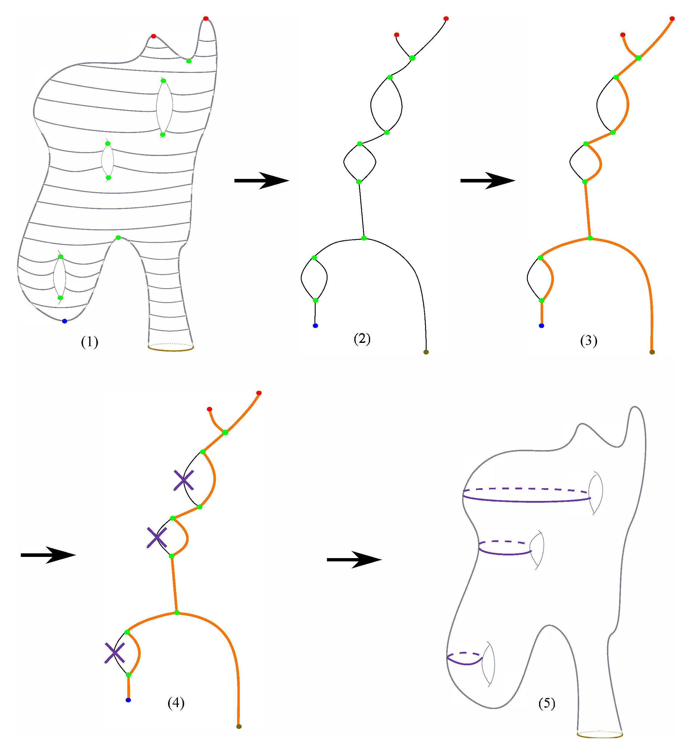
A Reeb graph naturally gives rise to a collection of curves that can be used to decompose a surface into a pair of pants. A pair of pants is a genus zero surface with three boundary components. Beside surface segmentation [87], surface pants decomposition has found applications in mesh parametrization [88], surface matching [89], and surface classification and indexing [90]. The method for obtaining a pants decomposition from the Reeb graph is illustrated in Figure 22 and is described, as follows:
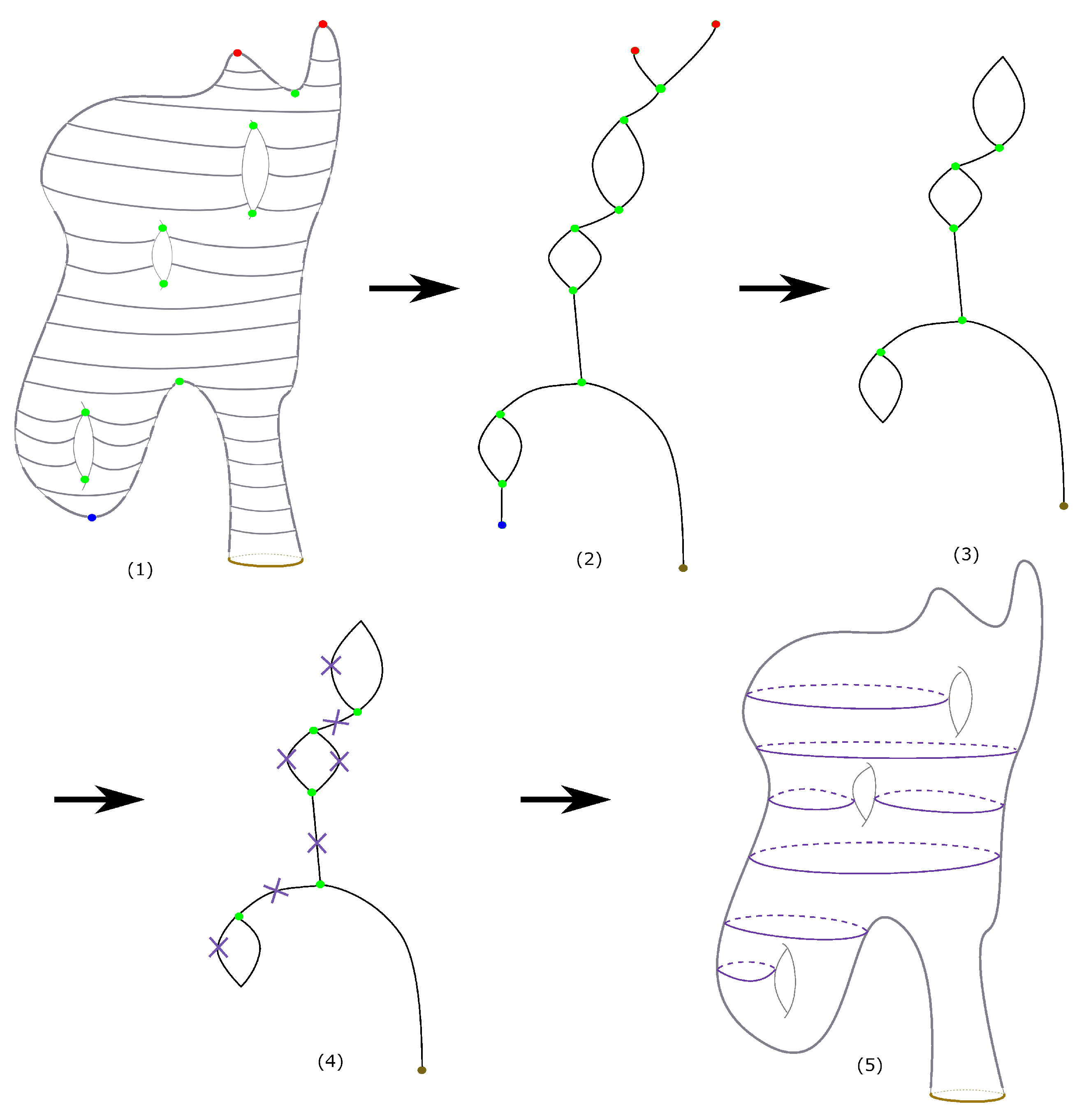
- Let be the deformation retract of . This graph can be obtained by recursively deleting nodes with valency one from and the edge attached to them until no such indices exist. We exclude from this deletion the 1-valence nodes originating from the boundary of M. We also delete all of the nodes with valency 2 and combine the two edges that meet at that node to form a single edge. This step is illustrated in step Figure 23.
- We select one interior point from each edge in , provided that this edge does not have a node of valency one.
- We use our Reeb algorithm to determine the curves on the surface that correspond to the points that we selected on the graph in the previous step.
The results of the previous algorithm were tested on triangulated meshes with various topological complexities. We show some examples in Figure 23.
Branch Curves.
A branch curve on a surface M is a simple closed curve that bounds a topological disk on M. Such a curve is also called null homotopic. A branch curve is determined by a Reeb graph edge, which has a vertex of valence one. Note that cutting the surface along a branch curve increases the number of connected components of the surface. Cutting along such curves can be used for the segmentation of a genus zero surfaces. There are many Reeb graph-based segmentation algorithms in the literature for segmentation of genus zero surfaces, such as the surface obtained from a humanoid character. See, for instance, [54,83,84]. Because this type of curves is essentially utilized elsewhere in the literature, we simply list it here for completeness of our discussion. However, all of these methods lack the description of a method to extract the manifold data from the Reeb graph data.
8.1. Choosing Morse Scalar Functions
The cutting system and pant decomposition curves that we presented in this section depend on the choice of the scalar function used to define the Reeb graph in the following way. In particular, the choice of these curves affects the final quality of the segmented mesh. For this reason, it is important to choose a scalar function with certain desirable properties. By desirable properties, we mean the following:
- The scalar function has a small number of critical vertices.
- The level sets of the scalar function follow the geometry of the mesh as closely as possible.
- The scalar function requires minimal input from the user.
We briefly discuss several scalar functions with the above properties.
8.1.1. Harmonic Functions
Condition 1 is desirable, because it leads, in general, to a simpler Reeb graph. For a surface mesh M of genus g one can always construct a scalar function f on M with critical points. This can be done by the so-called Harmonic functions. Recall that a harmonic map on a triangulated surface M is a scalar function that satisfies the Laplace equation subject to the Dirichlet boundary conditions for all . Here, the set is a list of constrained vertices and have known scalar values providing the boundary conditions. The reason for our interest in Harmonic functions is that they satisfy the so-called maximum principle property [91], which asserts that the solution for the above system has no local extrema other than the constrained vertices. To achieve this setting in practice, one has to be careful about the choice of the weights utilized to define the Laplacian. More specifically, for a triangulated mesh M, the standard discretization for the Laplacian operator at a vertex is given by:
where is a scalar weight assigned to the edge , such that . Choosing the weights , such that for all edges guarantees the solution of the Laplace equation has no local extrema other than at constrained vertices [92]. These conditions are satisfied by the mean value weights:
where the angles and are the angles on either sides of the edge at the vertex . Mean value weights are used to approximate harmonic map and they have the advantage that they are always non-negative, which prevents any introduction of extrema on non-constrained vertices in the solution of the Laplace equation that is specified above. Such a function can be obtained as a solution for Laplace equation with mean value weights and with only two constrained vertices such that . For instance, all functions shown in Figure 19 are obtained by solving the Laplace equation with exactly two constrained vertices.
8.1.2. The Poisson Equation
The Poisson equation on a triangulated mesh with Dirichlet boundary condition is defined by:
where is a set of constrained vertices and is a known function. The cardinality of the set must be at least 1 in order for system (1) to have a unique solution. With the appropriate choice of h, we can use the Poisson equation for our purpose. Indeed, if we choose the function h as suggested by Dong et al. in [93], then the solution f of the Poisson equation gives us a scalar field whose level sets follow one of the principal curvatures of the underlying manifold. Specifically, this can be done by solving:
where is the mean curvature at the vertex v:
here, the angles and are given in Figure 24, and is the surface mixed area around the vertex [94]. Examples of Poisson fields on triangulated meshes are shown in Figure 25.
9. Conclusions and Future Work
The parallelization of topological data analysis algorithms is still in its infancy. There are plenty of existing topological machineries, such as Morse theory, which offer a plethora of tools that can be utilized to obtain robust and efficient parallel algorithms. In this paper, we presented a work that utilizes Morse theory to obtain a parallel algorithm for augmented Reeb graphs.
The parallel algorithm that we present here has elements that make it generalizable to a Reeb graph algorithm on a general simplicial complex. However, we thought that this would make the discussion more complicated in many parts of the algorithm. We plan to pursue this direction in future work.
Author Contributions
Conceptualization, M.H. and P.R.; funding acquisition, P.R.; software, M.H. All authors have read and agreed to the published version of the manuscript.
Funding
This work was supported in part by the National Science Foundation (IIS-1513616 and IIS-1845204).
Conflicts of Interest
The authors declare no conflict of interest.
References
- Carlsson, G. Topology and data. Bull. Am. Math. Soc. 2009, 46, 255–308. [Google Scholar] [CrossRef] [Green Version]
- Carlsson, G.; Mémoli, F. Persistent clustering and a theorem of J. Kleinberg. arXiv 2008, arXiv:0808.2241. [Google Scholar]
- Reeb, G. Sur les Points Singuliers d’une Forme de Pfaff Completement Intergrable ou d’une Fonction Numerique (On the Singular Points of a Complete Integral Pfaff Form or of a Numerical Function). C. R. Acad. Sci. Paris 1946, 222, 847–849. [Google Scholar]
- Boyell, R.L.; Ruston, H. Hybrid techniques for real-time radar simulation. In AFIPS ’63 (Fall): Proceedings of the November 12–14, 1963, Fall Joint Computer Conference; Association for Computing Machinery: New York, NY, USA, 1963; pp. 445–458. [Google Scholar]
- Hétroy, F.; Attali, D. Topological quadrangulations of closed triangulated surfaces using the Reeb graph. Graph. Models 2003, 65, 131–148. [Google Scholar] [CrossRef] [Green Version]
- Attene, M.; Biasotti, S.; Spagnuolo, M. Shape understanding by contour-driven retiling. Vis. Comput. 2003, 19, 127–138. [Google Scholar] [CrossRef]
- Biasotti, S.; Falcidieno, B.; Spagnuolo, M. Extended reeb graphs for surface understanding and description. In Discrete Geometry for Computer Imagery; Springer: Berlin/Heidelberg, Germany, 2000; pp. 185–197. [Google Scholar]
- Patane, G.; Spagnuolo, M.; Falcidieno, B. Para-Graph: Graph-Based Parameterization of Triangle Meshes with Arbitrary Genus. In Computer Graphics Forum; Wiley Online Library: Hoboken, NJ, USA, 2004; Volume 23, pp. 783–797. [Google Scholar]
- Zhang, E.; Mischaikow, K.; Turk, G. Feature-based surface parameterization and texture mapping. ACM Trans. Graph. 2005, 24, 1–27. [Google Scholar] [CrossRef]
- Werghi, N.; Xiao, Y.; Siebert, J.P. A functional-based segmentation of human body scans in arbitrary postures. IEEE Trans. Syst. Man Cybern. Part B Cybern. 2006, 36, 153–165. [Google Scholar] [CrossRef] [Green Version]
- Kanongchaiyos, P.; Shinagawa, Y. Articulated Reeb graphs for interactive skeleton animation. In Multimedia Modeling: Modeling Multimedia Information and Systems; World Scientific: Singapore, 2000; pp. 451–467. [Google Scholar]
- Takahashi, S.; Takeshima, Y.; Fujishiro, I. Topological volume skeletonization and its application to transfer function design. Graph. Models 2004, 66, 24–49. [Google Scholar] [CrossRef]
- Carr, H.; Snoeyink, J.; van de Panne, M. Simplifying flexible isosurfaces using local geometric measures. In Proceedings of the IEEE Visualization, Austin, TX, USA, 10–15 October 2004; pp. 497–504. [Google Scholar]
- Rosen, P.; Wang, B.; Seth, A.; Mills, B.; Ginsburg, A.; Kamenetzky, J.; Kern, J.; Johnson, C.R. Using Contour Trees in the Analysis and Visualization of Radio Astronomy Data Cubes. arXiv 2017, arXiv:1704.04561. [Google Scholar]
- Kweon, I.S.; Kanade, T. Extracting topographic terrain features from elevation maps. CVGIP Image Underst. 1994, 59, 171–182. [Google Scholar] [CrossRef]
- Bajaj, C.; Pascucci, V.; Schikore, D. The contour spectrum. In Proceedings of the IEEE Visualization, Phoenix, AZ, USA, 24–24 October 1997; pp. 167–173. [Google Scholar]
- Harvey, W.; Wang, Y.; Wenger, R. A randomized O (m log m) time algorithm for computing Reeb graphs of arbitrary simplicial complexes. In SoCG ’10: Proceedings of the Twenty-Sixth Annual Symposium on Computational Geometry; ACM: New York, NY, USA, 2010; pp. 267–276. [Google Scholar]
- Shinagawa, Y.; Kunii, T.L. Constructing a Reeb graph automatically from cross sections. IEEE Comput. Graph. Appl. 1991, 11, 44–51. [Google Scholar] [CrossRef]
- Cole-McLaughlin, K.; Edelsbrunner, H.; Harer, J.; Natarajan, V.; Pascucci, V. Loops in Reeb graphs of 2-manifolds. In SCG ’03: Proceedings of the Nineteenth Annual Symposium on Computational Geometry; ACM: New York, NY, USA, 2003; pp. 344–350. [Google Scholar]
- Tierny, J.; Gyulassy, A.; Simon, E.; Pascucci, V. Loop surgery for volumetric meshes: Reeb graphs reduced to contour trees. IEEE Trans. Vis. Comput. Graph. 2009, 15, 1177–1184. [Google Scholar] [CrossRef]
- Chiang, Y.J.; Lenz, T.; Lu, X.; Rote, G. Simple and optimal output-sensitive construction of contour trees using monotone paths. Comput. Geom. 2005, 30, 165–195. [Google Scholar] [CrossRef] [Green Version]
- Edelsbrunner, H.; Harer, J.; Mascarenhas, A.; Pascucci, V. Time-varying reeb graphs for continuous space-time data. In SCG ’04: Proceedings of the Twentieth Annual Symposium on Computational Geometry; ACM: New York, NY, USA, 2004; pp. 366–372. [Google Scholar]
- Pascucci, V.; Scorzelli, G.; Bremer, P.T.; Mascarenhas, A. Robust on-line computation of Reeb graphs: Simplicity and speed. ACM Trans. Graph. 2007, 26, 58. [Google Scholar] [CrossRef]
- Doraiswamy, H.; Natarajan, V. Efficient algorithms for computing Reeb graphs. Comput. Geom. 2009, 42, 606–616. [Google Scholar] [CrossRef] [Green Version]
- Parsa, S. A deterministic O(m log m) time algorithm for the Reeb graph. In SoCG ’12: Proceedings of the Twenty-Eighth Annual Symposium on Computational Geometry; ACM: New York, NY, USA, 2012; pp. 269–276. [Google Scholar]
- Doraiswamy, H.; Natarajan, V. Efficient output-sensitive construction of Reeb graphs. In International Symposium on Algorithms and Computation; Springer: Berlin/Heidelberg, Germany, 2008; pp. 556–567. [Google Scholar]
- Hilaga, M.; Shinagawa, Y.; Kohmura, T.; Kunii, T.L. Topology matching for fully automatic similarity estimation of 3D shapes. In SIGGRAPH ’01: Proceedings of the 28th Annual Conference on Computer Graphics and Interactive Techniques; ACM: New York, NY, USA, 2001; pp. 203–212. [Google Scholar]
- Ge, X.; Safa, I.I.; Belkin, M.; Wang, Y. Data skeletonization via Reeb graphs. In Proceedings of the Advances in Neural Information Processing Systems, Granada, Spain, 13–15 December 2011; pp. 837–845. [Google Scholar]
- Tung, T.; Schmitt, F. Augmented reeb graphs for content-based retrieval of 3d mesh models. In Proceedings of the Shape Modeling Applications, Genova, Italy, 7–9 June 2004; pp. 157–166. [Google Scholar]
- Biasotti, S.; Giorgi, D.; Spagnuolo, M.; Falcidieno, B. Reeb graphs for shape analysis and applications. Theor. Comput. Sci. 2008, 392, 5–22. [Google Scholar] [CrossRef] [Green Version]
- Raichel, B.; Seshadhri, C. Avoiding the global sort: A faster contour tree algorithm. arXiv 2014, arXiv:1411.2689. [Google Scholar] [CrossRef] [Green Version]
- Van Kreveld, M.; van Oostrum, R.; Bajaj, C.; Pascucci, V.; Schikore, D. Contour trees and small seed sets for isosurface traversal. In SCG ’97: Proceedings of the Thirteenth Annual Symposium on Computational Geometry; ACM: New York, NY, USA, 1997; pp. 212–220. [Google Scholar]
- Tarasov, S.P.; Vyalyi, M.N. Construction of contour trees in 3D in O (n log n) steps. In SSCG ’98: Proceedings of the Fourteenth Annual Symposium on Computational Geometry; ACM: New York, NY, USA, 1998; pp. 68–75. [Google Scholar]
- Pascucci, V.; Cole-McLaughlin, K.; Scorzelli, G. Multi-resolution computation and presentation of contour trees. In Proceedings of the IASTED International Conference on Visualization, Imaging, and Image Processing, Marbella, Spain, 6–8 September 2004. [Google Scholar]
- Weber, G.; Scheuermann, G. Topology-based transfer function design. In Proceedings of the IASTED International Conference on Visualization, Imaging, and Image Processing, Marbella, Spain, 3–5 September 2002; pp. 527–532. [Google Scholar]
- Besl, P.J.; McKay, N.D. Method for registration of 3-D shapes. In Proceedings of the Sensor fusion IV: Control paradigms and data structures, Boston, MA, USA, 30 April 1992; pp. 586–606. [Google Scholar]
- Gupta, S.K.; Regli, W.C.; Nau, D.S. Manufacturing feature instances: Which ones to recognize? In SMA ’95: Proceedings of the Third ACM Symposium on Solid Modeling and Applications; ACM: New York, NY, USA, 1995; pp. 141–152. [Google Scholar]
- Gueunet, C.; Fortin, P.; Jomier, J. Contour forests: Fast multi-threaded augmented contour trees. In Proceedings of the IEEE Symposium on Large Data Analysis and Visualization (LDAV), Baltimore, MD, USA, 23–28 October 2016; pp. 85–92. [Google Scholar]
- Carr, H. Topological Manipulation of Isosurfaces. Ph.D. Thesis, University of British Columbia, Vancouver, BC, Canada, 2004. [Google Scholar]
- Dey, T.K.; Sun, J.; Wang, Y. Approximating cycles in a shortest basis of the first homology group from point data. Inverse Probl. 2011, 27, 124004. [Google Scholar] [CrossRef]
- Chazal, F.; Oudot, S. Towards persistence-based reconstruction in Euclidean spaces. In SCG ’08: Proceedings of the Twenty-Fourth Annual Symposium on Computational Geometry; ACM: New York, NY, USA, 2008; pp. 232–241. [Google Scholar]
- Dey, T.K.; Li, K. Cut locus and topology from surface point data. In SCG ’09: Proceedings of the Twenty-Fifth Annual Symposium on Computational Geometry; ACM: New York, NY, USA, 2009; pp. 125–134. [Google Scholar]
- Natali, M.; Biasotti, S.; Patanè, G.; Falcidieno, B. Graph-based representations of point clouds. Graph. Models 2011, 73, 151–164. [Google Scholar] [CrossRef]
- Chazal, F.; Guibas, L.J.; Oudot, S.; Skraba, P. Analysis of scalar fields over point cloud data. In Proceedings of the ACM-SIAM Symposium on Discrete Algorithms, New York, NY, USA, 4–6 January 2009; pp. 1021–1030. [Google Scholar]
- Singh, G.; Mémoli, F.; Carlsson, G. Topological methods for the analysis of high dimensional data sets and 3d object recognition. In Eurographics/IEEE VGTC Symposium on Point-Based Graphics; The Eurographics Association: Munich, Germany, 2007; pp. 91–100. [Google Scholar]
- Lum, P.; Singh, G.; Lehman, A.; Ishkanov, T.; Vejdemo-Johansson, M.; Alagappan, M.; Carlsson, J.; Carlsson, G. Extracting insights from the shape of complex data using topology. Sci. Rep. 2013, 3, 1236. [Google Scholar] [CrossRef] [Green Version]
- Nicolau, M.; Levine, A.J.; Carlsson, G. Topology based data analysis identifies a subgroup of breast cancers with a unique mutational profile and excellent survival. Proc. Natl. Acad. Sci. USA 2011, 108, 7265–7270. [Google Scholar] [CrossRef] [PubMed] [Green Version]
- Robles, A.; Hajij, M.; Rosen, P. The Shape of an Image: A Study of Mapper on Images. In Proceedings of the International Conference on Computer Vision Theory and Applications (VISAPP), Funchal, Portugal, 27–29 January 2018. [Google Scholar]
- Rosen, P.; Hajij, M.; Tu, J.; Arafin, T.; Piegl, L. Inferring Quality in Point Cloud-based 3D Printed Objects using Topological Data Analysis. Comput.-Aided Des. Appl. 2019, 16, 519–527. [Google Scholar] [CrossRef]
- Carrière, M.; Oudot, S. Structure and stability of the 1-dimensional mapper. arXiv 2015, arXiv:1511.05823. [Google Scholar]
- Dey, T.K.; Memoli, F.; Wang, Y. Topological Analysis of Nerves, Reeb Spaces, Mappers, and Multiscale Mappers. arXiv 2017, arXiv:1703.07387. [Google Scholar]
- Munch, E.; Wang, B. Convergence between categorical representations of reeb space and mapper. arXiv 2015, arXiv:1512.04108. [Google Scholar]
- Hajij, M.; Wang, B.; Rosen, P. MOG: Mapper on Graphs for Relationship Preserving Clustering. arXiv 2018, arXiv:1804.11242. [Google Scholar]
- Xiao, Y.; Siebert, J.P.; Werghi, N. A discrete Reeb graph approach for the segmentation of human body scans. In Proceedings of the International Conference on 3-D Digital Imaging and Modeling (3DIM), Banff, AB, Canada, 6–10 October 2003; pp. 378–385. [Google Scholar]
- Tung, T.; Schmitt, F. The augmented multiresolution Reeb graph approach for content-based retrieval of 3D shapes. Int. J. Shape Model. 2005, 11, 91–120. [Google Scholar] [CrossRef]
- Mohamed, W.; Hamza, A.B. Reeb graph path dissimilarity for 3D object matching and retrieval. Vis. Comput. 2012, 28, 305–318. [Google Scholar] [CrossRef]
- Biasotti, S.; Mortara, M.; Spagnuolo, M. Surface compression and reconstruction using Reeb graphs and shape analysis. In Proceedings of the Spring Conference on Computer Graphics, Budmerice, Slovakia, 3–6 May 2000; pp. 174–185. [Google Scholar]
- Dey, T.K.; Li, K.; Sun, J.; Cohen-Steiner, D. Computing geometry-aware handle and tunnel loops in 3D models. ACM Trans. Graph. 2008, 27, 45. [Google Scholar] [CrossRef] [Green Version]
- Wood, Z.; Hoppe, H.; Desbrun, M.; Schröder, P. Removing excess topology from isosurfaces. ACM Trans. Graph. 2004, 23, 190–208. [Google Scholar] [CrossRef]
- Lewis, R.H.; Zomorodian, A. Multicore Homology via Mayer Vietoris. arXiv 2014, arXiv:1407.2275. [Google Scholar]
- Lipsky, D.; Skraba, P.; Vejdemo-Johansson, M. A spectral sequence for parallelized persistence. arXiv 2011, arXiv:1112.1245. [Google Scholar]
- Morozov, D.; Weber, G. Distributed contour trees. In Topological Methods in Data Analysis and Visualization III; Springer: Cham, Switzerland, 2012. [Google Scholar]
- Morozov, D.; Weber, G. Distributed merge trees. In Proceedings of the 18th ACM SIGPLAN Symposium on Principles and Practice of Parallel Programming, Shenzhen, China, 23–27 February 2013; Volume 48, pp. 93–102. [Google Scholar]
- Masood, T.B.; Ray, T.; Natarajan, V. Parallel computation of alpha complexes for biomolecules. Comput. Geom. 2020, 90, 101651. [Google Scholar] [CrossRef]
- Hajij, M.; Assiri, B.; Rosen, P. Distributed Mapper. arXiv 2017, arXiv:1712.03660. [Google Scholar]
- Matsumoto, Y. An Introduction to Morse Theory; American Mathematical Society: Providence, RI, USA, 2002; Volume 208. [Google Scholar]
- Banyaga, A.; Hurtubise, D. Lectures on Morse Homology; Springer Science & Business Media: New York, NY, USA, 2013; Volume 29. [Google Scholar]
- Morse, M. The Calculus of Variations in the Large; American Mathematical Society: Providence, RI, USA, 1934; Volume 18. [Google Scholar]
- Milnor, J.W. Morse Theory; Number 51; Princeton University Press: Princeton, NJ, USA, 1963. [Google Scholar]
- Banchoff, T. Critical points and curvature for embedded polyhedra. J. Diff. Geom. 1967, 1, 245–256. [Google Scholar] [CrossRef]
- Guo, X.; Li, X.; Bao, Y.; Gu, X.; Qin, H. Meshless thin-shell simulation based on global conformal parameterization. IEEE Trans. Vis. Comput. Graph. 2006, 12, 375–385. [Google Scholar] [PubMed]
- Ni, X.; Garland, M.; Hart, J.C. Fair morse functions for extracting the topological structure of a surface mesh. ACM Trans. Graph. 2004, 23, 613–622. [Google Scholar] [CrossRef]
- Dong, S.; Bremer, P.T.; Garland, M.; Pascucci, V.; Hart, J.C. Spectral surface quadrangulation. ACM Trans. Graph. 2006, 25, 1057–1066. [Google Scholar] [CrossRef]
- Stander, B.T.; Hart, J.C. Guaranteeing the topology of an implicit surface polygonization for interactive modeling. In SIGGRAPH ’97: Proceedings of the 24th Annual Conference on Computer Graphics and Interactive Techniques; ACM Press: New York, NY, USA, 1997; pp. 279–286. [Google Scholar]
- Yamazaki, I.; Natarajan, V.; Bai, Z.; Hamann, B. Segmenting point sets. In Proceedings of the IEEE International Conference on Shape Modeling and Applications 2006, Matsushima, Japan, 14–16 June 2006; p. 6. [Google Scholar]
- Wang, H.; He, Y.; Li, X.; Gu, X.; Qin, H. Geometry-aware domain decomposition for T-spline-based manifold modeling. Comput. Graph. 2009, 33, 359–368. [Google Scholar] [CrossRef]
- Tsigas, P.; Zhang, Y. A simple, fast parallel implementation of quicksort and its performance evaluation on SUN enterprise 10000. In Proceedings of the Euromicro Conference on Parallel, Distributed, and Network-Based Processing, Genova, Italy, 5–7 February 2003; pp. 372–381. [Google Scholar]
- Singler, J.; Sanders, P.; Putze, F. MCSTL: The multi-core standard template library. In European Conference on Parallel Processing; Springer: Berlin/Heidelberg, Germany, 2007; pp. 682–694. [Google Scholar]
- Pinkall, U.; Polthier, K. Computing discrete minimal surfaces and their conjugates. Exp. Math. 1993, 2, 15–36. [Google Scholar] [CrossRef]
- Polthier, K. Polyhedral Surfaces of Constant Mean Curvature. Ph.D. Thesis, Habilitationsschrift TU, Berlin, Germany, 2002. [Google Scholar]
- Crane, K.; Weischedel, C.; Wardetzky, M. Geodesics in heat: A new approach to computing distance based on heat flow. ACM Trans. Graph. 2013, 32, 1–11. [Google Scholar] [CrossRef]
- Sumner, R.W.; Popović, J. Deformation transfer for triangle meshes. ACM Trans. Graph. 2004, 23, 399–405. [Google Scholar] [CrossRef]
- Xiao, Y.; Werghi, N.; Siebert, J.P. A topological approach for segmenting human body shape. In Proceedings of the International Conference on Image Analysis and Processing, Mantova, Italy, 17–19 September 2003; pp. 82–87. [Google Scholar]
- Tierny, J.; Vandeborre, J.P.; Daoudi, M. Topology driven 3D mesh hierarchical segmentation. In Proceedings of the IEEE International Conference on Shape Modeling and Applications 2007 (SMI ’07), Lyon, France, 13–15 June 2007; pp. 215–220. [Google Scholar]
- Hatcher, A.; Thurston, W. A presentation for the mapping class group of a closed orientable surface. Topology 1980, 19, 221–237. [Google Scholar] [CrossRef] [Green Version]
- Zeng, W.; Yin, X.; Zhang, M.; Luo, F.; Gu, X. Generalized Koebe’s method for conformal mapping multiply connected domains. In SIAM/ACM Joint Conference on Geometric and Physical Modeling; ACM: New York, NY, USA, 2009; pp. 89–100. [Google Scholar]
- Hajij, M.; Dey, T.; Li, X. Segmenting a surface mesh into pants using Morse theory. Graph. Models 2016, 88, 12–21. [Google Scholar] [CrossRef] [Green Version]
- Kwok, T.H.; Zhang, Y.; Wang, C.C. Constructing common base domain by cues from Voronoi diagram. Graph. Models 2012, 74, 152–163. [Google Scholar] [CrossRef]
- Li, X.; Gu, X.; Qin, H. Surface mapping using consistent pants decomposition. IEEE Trans. Vis. Comput. Graph. 2009, 15, 558–571. [Google Scholar] [CrossRef]
- Jin, M.; Zeng, W.; Ding, N.; Gu, X. Computing Fenchel-Nielsen coordinates in teichmuller shape space. In Proceedings of the 2009 IEEE International Conference on Shape Modeling and Applications, Beijing, China, 26–28 June 2009; pp. 193–200. [Google Scholar]
- Rosenberg, S. The Laplacian on a Riemannian Manifold: An Introduction to Analysis on Manifolds; Number 31; Cambridge University Press: Cambridge, UK, 1997. [Google Scholar]
- Floater, M.S. Mean value coordinates. Comput. Aided Geom. Des. 2003, 20, 19–27. [Google Scholar] [CrossRef]
- Dong, S.; Kircher, S.; Garland, M. Harmonic functions for quadrilateral remeshing of arbitrary manifolds. Comput. Aided Geom. Des. 2005, 22, 392–423. [Google Scholar] [CrossRef]
- Meyer, M.; Desbrun, M.; Schröder, P.; Barr, A.H. Discrete differential-geometry operators for triangulated 2-manifolds. In Visualization and Mathematics III; Springer: Berlin/Heidelberg, Germany, 2003; pp. 35–57. [Google Scholar]
Figure 1.
Minimum, Saddle, and Maximum, respectively.

Figure 2.
An example of a Reeb graph (right) of a scalar function (left) defined on a surface with a boundary.
Figure 2.
An example of a Reeb graph (right) of a scalar function (left) defined on a surface with a boundary.

Figure 3.
The types of vertices on a triangulated mesh. From left to right: minimum, maximum, regular vertex, and saddle.
Figure 3.
The types of vertices on a triangulated mesh. From left to right: minimum, maximum, regular vertex, and saddle.

Figure 4.
For a critical value, on the left, the set consists of a singular set and two of simple closed curves. On the right, only the critical set is shown, which is the connected component of that contains the critical point p.
Figure 4.
For a critical value, on the left, the set consists of a singular set and two of simple closed curves. On the right, only the critical set is shown, which is the connected component of that contains the critical point p.

Figure 5.
A split saddle on the left and a merge saddle on the right.

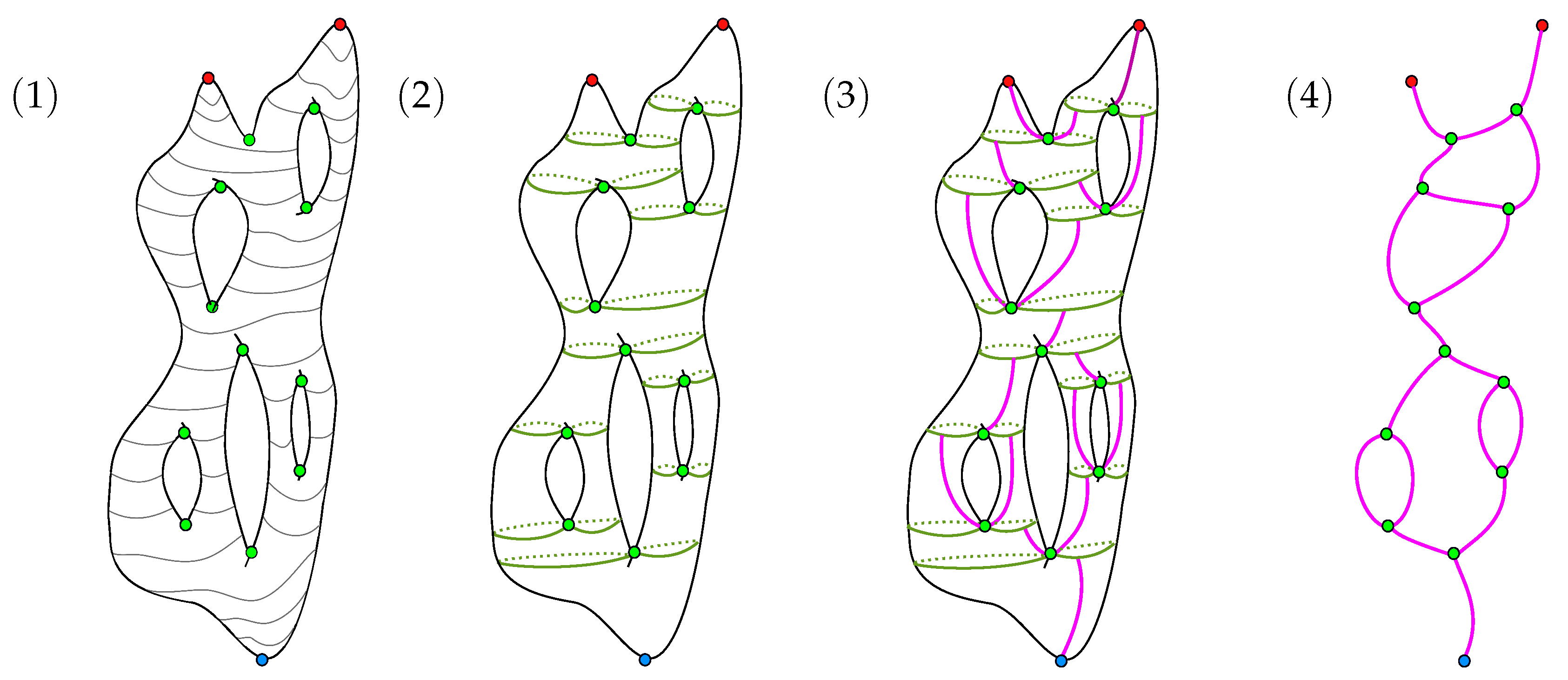
Figure 6.
Summary of the sequential algorithm. (1) The input of the algorithm is a manifold M with a scalar function f. (2) Computing the critical sets. (3) For each saddle point or minimum, we compute the ascending paths (4) creating the edges of the Reeb graph by the information encoded in the start vertex of the ascending vertex and its termination critical set.

Figure 7.
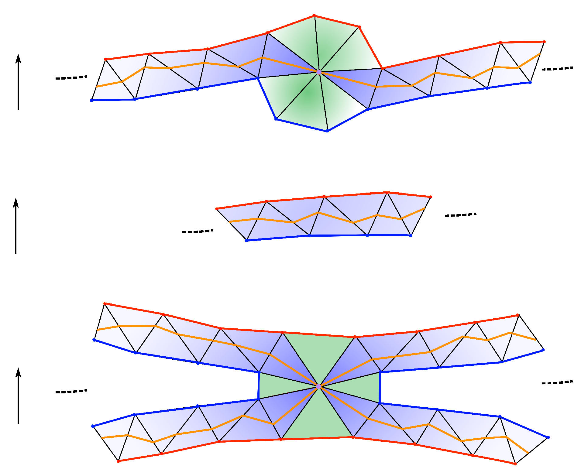
The set of vertices, edges, and faces in the mesh M, which intersects. The top two figures depict cases where t is a regular value. The top figure shows an example of when there exists a vertex v in M, such that . The second figure shows the case where no such a vertex exists. In other words, intersects only edges and faces of M. The third figure is an example of the local neighborhood, a critical point of f or when contains a critical point. The purple simplices represent the set . The union of the green and purple simplices represents the set . The blue edges and nodes are the edges in the complexes that are shown in the figure and nodes in , which have f-values less than or equal to t. The red edges and nodes are the edges in the complexes shown in the figure and nodes in , which have f-values that are higher than or equal to t.
Figure 7.
The set of vertices, edges, and faces in the mesh M, which intersects. The top two figures depict cases where t is a regular value. The top figure shows an example of when there exists a vertex v in M, such that . The second figure shows the case where no such a vertex exists. In other words, intersects only edges and faces of M. The third figure is an example of the local neighborhood, a critical point of f or when contains a critical point. The purple simplices represent the set . The union of the green and purple simplices represents the set . The blue edges and nodes are the edges in the complexes that are shown in the figure and nodes in , which have f-values less than or equal to t. The red edges and nodes are the edges in the complexes shown in the figure and nodes in , which have f-values that are higher than or equal to t.

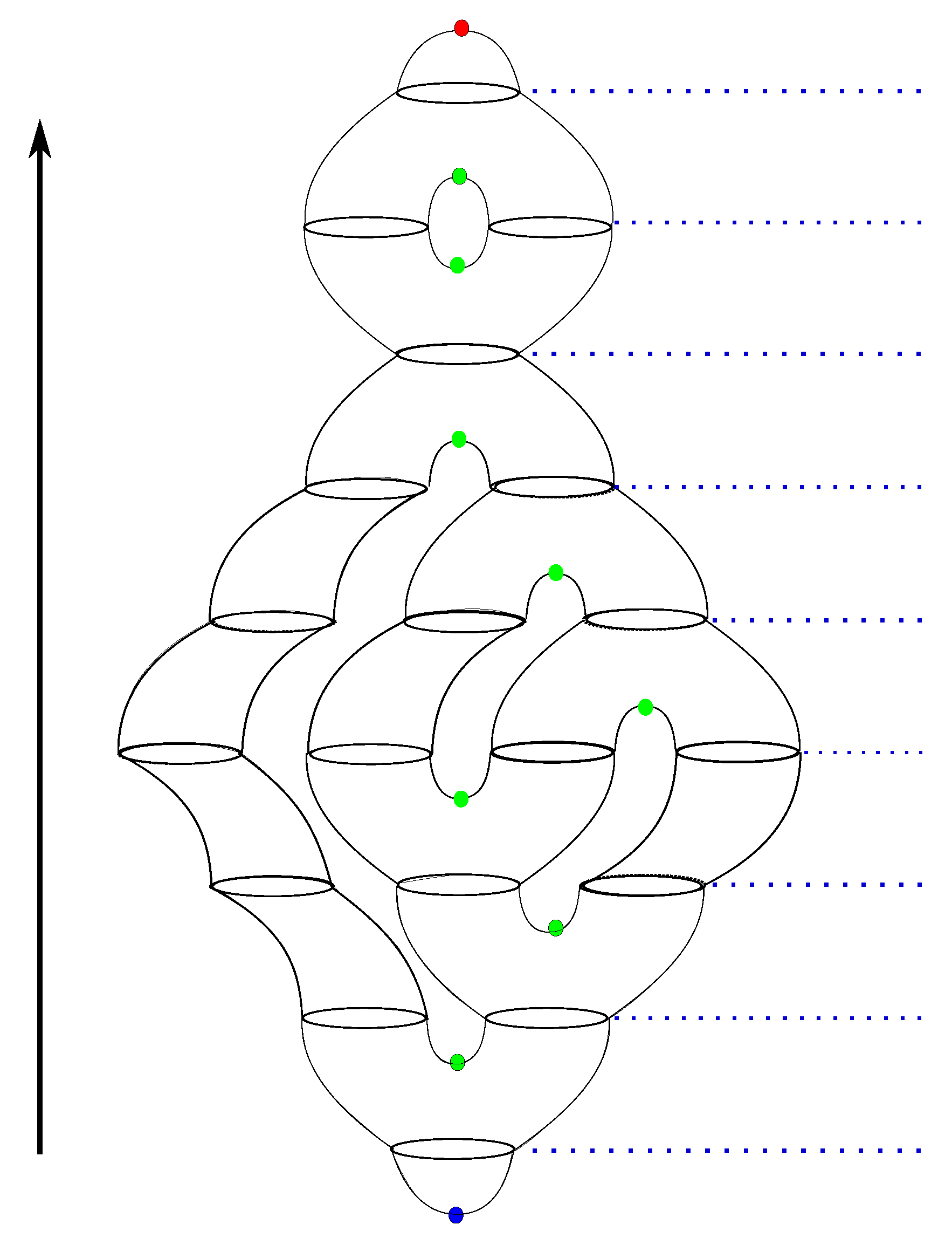
Figure 8.
Given a Morse function f on a surface M, we can slice M, so that, around each critical value t, the submanifold is a disjoint union of simple building blocks: pair of pants, topological cylinders, and topological disks.
Figure 8.
Given a Morse function f on a surface M, we can slice M, so that, around each critical value t, the submanifold is a disjoint union of simple building blocks: pair of pants, topological cylinders, and topological disks.

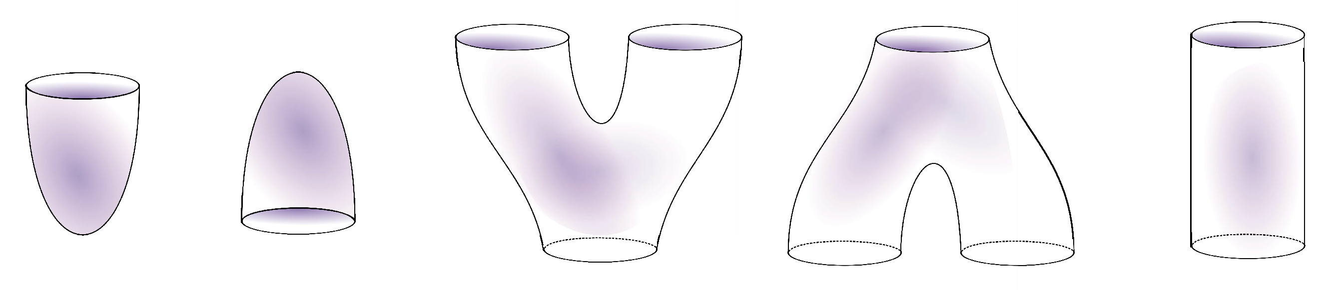
Figure 9.
The building blocks of a surface. Given a scalar function f defined on a surface M, Theorem 2 asserts that we can decompose the surface into the building block pieces appear in above. These pieces are genus zero surfaces with a single boundary component (disk), genus zero surfaces with three boundary components (pair of pants), and a genus zero surface with two boundary components (cylinder).

Figure 10.
The restriction of the Reeb graph on the building blocks of a surface along with the part of the ascending paths in that part of the surface. Around each critical point, the structure of the ascending curves (orange) is identical to the structure of the Reeb graph. More precisely, the quotient space of the restriction of the function on the ascending curves the critical sets around a critical point (these are the curves highlighted by orange and red in the figure) is identical to the quotient space of the manifold locally.

Figure 11.
An illustration of the partition stage. (a) A connected component of the submanifold is obtained. (b) is extended to by adding the crossing edges. (c) A closeup of the crossing edges of the manifold . The blue edges represent the crossings edges of and the green curve represents the portion of the curve within the closeup region.

Figure 12.
An illustration of the gluing stage. (a) At this stage, two ascending paths from all submanifolds have been calculated. In the case when two consecutive submanifolds share a crossing edge, such as the case in the illustrative figure, the ascending path of the lower submanifold gets terminated at the at a crossing edge. Similarly, an ascending path from the higher submanifold gets initiated at a crossing edge. (b) A zoomed version of Figure (a) shows the two crossing edges that determine uniquely two nodes in the Reeb graphs and . The fact that these two edges belong to the same connected component in the inverse image of the regular crossing value is used to glue the graphs and along the blue nodes to obtain the graph in Figure (c).

Figure 13.
An illustration of the data retrieval procedure. (1) A value is selected from the interval . (2) This value is used to determine a point p on the Reeb graph edge . (3) This point is contained in an edge on the mesh M. This edge is used to determine the circle
Figure 13.
An illustration of the data retrieval procedure. (1) A value is selected from the interval . (2) This value is used to determine a point p on the Reeb graph edge . (3) This point is contained in an edge on the mesh M. This edge is used to determine the circle

Figure 14.
The arm of the female character mesh corresponds to a single arc in the Reeb graph associated with the scalar function indicated on the mesh. Observe that the gradient of this scalar function varies along this arm, which makes it hard to parametrize the mapping between the Reeb graph and the corresponding regions on the mesh.

Figure 15.
The gradients of hat functions of a triangle.

Figure 16.
Computing the divergence at vertex .

Figure 17.
Obtaining a unit gradient scalar field.

Figure 18.
Speedups obtained by our parallel Reeb graph algorithm.

Figure 19.
Some of the meshes that we used for our parallel Reeb graph computations.

Figure 20.
The steps of the cutting system algorithm. (1) mesh M with a scalar function defined on it are given. (2) The Reeb graph is computed. (3) We compute a spanning tree of . (4) We select all edges in the graph that do not belong the spanning tree we computed in (3) and then we select an interior point on each one of these edges. (5) For each interior point, we used our augmented Reeb graph algorithm to compute the circle that corresponds to it on the mesh.

Figure 21.
Examples of cut system curves on triangulated surfaces.

Figure 22.
A Reeb graph can be used to segment a surface into a collection of topologically consistent patches. (1) The surface M, with a scalar function f, is given as an input. (2) The Reeb graph of is calculated. (3) The deformation retract graph of the graph is calculated. (4) For each edge in the graph , we select a point. (5) We select the curves on the manifold M that corresponds to the points that were selected in the previous step.

Figure 23.
Examples of segmentation of higher genus surfaces into a pair of pants using our Reeb graph algorithm.
Figure 23.
Examples of segmentation of higher genus surfaces into a pair of pants using our Reeb graph algorithm.

Figure 24.
The angles and are defined with respect to an edge .

Figure 25.
Example of Poisson fields on Triangulated meshes. In both characters, a single vertex, which is the highest node in the head of the character, was chosen to be the constrained vertex required to solve the Poisson equation. Observe how this scalar function follows the geometry of the mesh.

© 2020 by the authors. Licensee MDPI, Basel, Switzerland. This article is an open access article distributed under the terms and conditions of the Creative Commons Attribution (CC BY) license (http://creativecommons.org/licenses/by/4.0/).
Share and Cite
MDPI and ACS Style
Hajij, M.; Rosen, P. An Efficient Data Retrieval Parallel Reeb Graph Algorithm. Algorithms 2020, 13, 258. https://0-doi-org.brum.beds.ac.uk/10.3390/a13100258
AMA Style
Hajij M, Rosen P. An Efficient Data Retrieval Parallel Reeb Graph Algorithm. Algorithms. 2020; 13(10):258. https://0-doi-org.brum.beds.ac.uk/10.3390/a13100258
Chicago/Turabian StyleHajij, Mustafa, and Paul Rosen. 2020. "An Efficient Data Retrieval Parallel Reeb Graph Algorithm" Algorithms 13, no. 10: 258. https://0-doi-org.brum.beds.ac.uk/10.3390/a13100258
Note that from the first issue of 2016, this journal uses article numbers instead of page numbers. See further details here.