Investigating Social Contextual Factors in Remaining-Time Predictive Process Monitoring—A Survival Analysis Approach


School of Computer Science and Engineering, University of Westminster, London W1W 6UW, UK
*
Author to whom correspondence should be addressed.
Algorithms 2020, 13(11), 267; https://0-doi-org.brum.beds.ac.uk/10.3390/a13110267
Submission received: 17 September 2020
/
Revised: 14 October 2020
/
Accepted: 19 October 2020
/
Published: 22 October 2020
(This article belongs to the Special Issue Process Mining and Emerging Applications)
Abstract
:Predictive process monitoring aims to accurately predict a variable of interest (e.g., remaining time) or the future state of the process instance (e.g., outcome or next step). The quest for models with higher predictive power has led to the development of a variety of novel approaches. However, though social contextual factors are widely acknowledged to impact the way cases are handled, as yet there have been no studies which have investigated the impact of social contextual features in the predictive process monitoring framework. These factors encompass the way humans and automated agents interact within a particular organisation to execute process-related activities. This paper seeks to address this problem by investigating the impact of social contextual features in the predictive process monitoring framework utilising a survival analysis approach. We propose an approach to censor an event log and build a survival function utilising the Weibull model, which enables us to explore the impact of social contextual factors as covariates. Moreover, we propose an approach to predict the remaining time of an in-flight process instance by using the survival function to estimate the throughput time for each trace, which is then used with the elapsed time to predict the remaining time for the trace. The proposed approach is benchmarked against existing approaches using five real-life event logs and it outperforms these approaches.
1. Introduction
Effectively predicting process outcomes in operational business management is essential for customer relationship management (e.g., ‘will this customer’s order be completed on time?’), enterprise resource planning (e.g., ‘what level of resourcing will be required to manage running cases/process instances?’) and operational process improvement (e.g., ‘what are the common attributes of cases that consistently complete late?’), among others. Predicting the remaining time of a process instance is also very useful. It is essential for effective scheduling of sequentially dependent processes and is a crucial determinant of consumer choice (e.g., where two or more services are identical in price and quality).
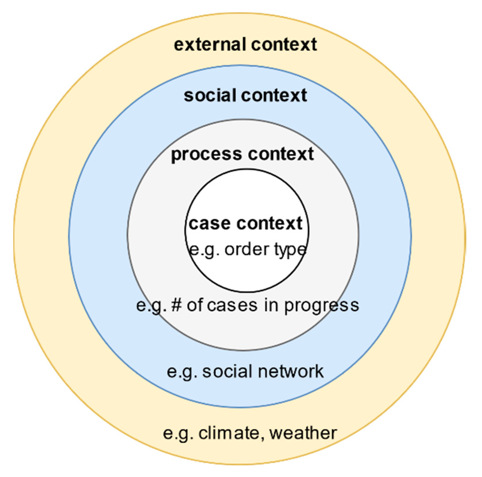
Reference [1] highlights the importance of contextual factors in predictive process monitoring and identifies four pertinent contextual types:
- Case context: the properties or attributes of a case.
- Process context: similar cases that may be competing for the same resources.
- Social context: the way human resources collaborate in an organisation to work on the process of interest.
- External context: factors in the broader ecosystem that impacts the process, e.g., weather, legislation, and location.
Figure 1 shows the relationship between the various contextual types.
To highlight the importance of social contextual factors, [1] argues that “activities are executed by people that operate in a social network. Friction between individuals may delay process instance, and the speed at which people work may vary.” It further adds that “process mining techniques tend to neglect the social context even though it is clear that this context directly impacts the way cases are handled”. The same argument could be made about process monitoring. This study aims to address that gap by empirically investigating the impact of social contextual factors in the predictive process monitoring workflow.
To date, numerous approaches have been used to predict process remaining time, including deep learning [2], queuing theory [3] and annotated transition systems [4], among others. This study uses the survival analysis approach, also referred to as “time-to-event” analysis. This approach dates back to work by John Graunt published in his 1662 book ‘Natural and Political Observations upon the Bill of Mortality’ which suggested that the time of death should be considered an event that deserved systematic study [5]. While the majority of applications of the approach have been in the healthcare research field, by replacing the event of “death” with other events, the approach has been successfully applied in others fields, such as human resources management to determine the time-to-employee-attrition [6], marketing to model time-to-customer-churn [7], and credit risk management to determine the time-to-default [8]. However, as yet, time-to-event methods have not been utilised in predictive process monitoring. This study intends to address that gap by proposing an approach that uses survival analysis to predict the remaining time for process instances from several event logs. The primary advantage survival analysis offers over other approaches is that it can deal well with censored observations, i.e., observations where time to the event of interest is unavailable. This contrasts with standard regression approaches which tend to produce results that are neither accurate nor reliable if a high percentage of cases are incomplete. Moreover, survival analysis approaches can handle covariates well. We propose a method for censoring event log for use in survival analysis by treating the completion of a process instance as the event of interest.
A review of the literature reveals three primary predictive process monitoring approaches: model-based approaches [4,9], sequence-to-feature encoding (STEP) approaches [10,11], and simulation-based approaches [12,13].
STEP approaches encode event log into feature-outcome pairs using a variety of techniques such as last state, aggregation, index-based or tensor encoding [11,14]. However, it is worth mentioning a subset of STEP approaches that have become popular in recent years, i.e., neural network-based approaches [2,15,16,17]. These state-of-the-art models make it relatively easy to include additional features into the prediction model. While the majority of these approaches focus on the next activity as the prediction target, the approach proposed by [2] utilises an LSTM (a particular type of a recurrent neural network) to iteratively predict the remaining activities till case completion and associated timestamps. This enables estimation of the remaining time of the process instance.
With regard to social contextual factors, [18] proposes an approach for discovering social networks from an event log and several metrics based on potential causality, joint cases/activities and special event types. They also apply these concepts to a real-life event log. In [19], the authors build on these and extend the approach to discover organisational models from event logs. In [20], the authors explore the relationship between the effect of workload and service time utilising regression analysis on historical event log data. In [21], the authors extend the standard network centrality measures (degree, closeness and betweenness centrality) which had hitherto been applied to individuals to groups and classes as well.
With regard to survival analysis, [22] compares approaches that utilise linear regression and survival analysis to model loan recovery rate and amounts. The authors propose an approach to determine the optimal quantile for taking a point estimate from the survival curve. In [9], the authors extend that approach to predict the time-to-default for credit data sets from Belgian and UK financial institutions.
In this paper, we utilise the STEP approach together with a survival analysis technique to build a predictive process monitoring framework utilising the Weibull model.
The remainder of the paper is structured as follows. Section 2 defines vital terms built on throughout the paper and describes the proposed approach, while Section 3 details the evaluation results of the proposed approach. The penultimate section summarises the findings and describes the threats to the validity of the study, while the final section suggests further research areas for extending these.
2. Materials and Methods
2.1. Definitions
2.1.1. Event, Traces and Event Logs
Several key terms to be built on throughout this review are formally defined. We adopt the standard notation defined in [1].
Definition 1.
Event. Let ε represents the event universe and Τ the time domain, A represents the set of activities, and P represents the set of performers (i.e., individuals and teams).
An event e is a tuple (#case_identifier(e), #activity(e), #start_time(e), #completion_time(e), #attribute1(e)..#attributen(e)). The elements of the tuple represent the attributes associated with the event. Though an event is minimally defined by the triplet ((#case_identifier(e), #activity(e), #completion_time(e)), it is common and desirable to have additional attributes such as #performer(e) indicating the performer associated with the event and #trans(e) indicating the transaction type associated with the event, amongst others. For each of these attributes, there is a function which assigns the attribute to the event. e.g., attrstart_time assigning a start time to the event, attrcompletion_time assigning a completion time to the event, attractivity assigning an activity label to the event and attrperformer , a partial function assigning a performer (or resource) to events. Note that attrperformer is a partial function as some events may not be associated with any performers.
An event is often identified by the activity label (#activity(e)) which describes the work performed on a process instance (or case) that transforms input(s) to output(s).
Definition 2.
Terminal activities. Letrepresent the set of valid terminal activity labels.
where en is a valid terminal event if #activity_label(en) This event indicates a ‘clean’ completion of the process instance. Otherwise, the process instance is still in-flight or abandoned.
Definition 3.
Trace. A trace is a (time-increasing) sequence of events, σ ∈ ε ∗ such that each event appears only once, i.e., for 1 ≤ i < j ≤ |σ|: σi ≠ σj and ≤ .
A partial trace (σp) has a non-valid terminal event as the final event (). It indicates an in-flight (pre-mortem) process instance.
A full trace (σf) ends with a terminal event (). It details the journey through the value chain that the particular process instance followed and indicates a completed (post-mortem) process instance.
Definition 4.
Censored traces. Let C represent the set of all possible traces and #censored(σ) represent a binary variable indicating whether a trace is censored or not respectively. A functionwhich assigns the appropriate value to a trace is defined as follows:
Definition 5.
Event log. An event log is a set of traces (full and partial) L for a particular process such that each event appears at least once in the log, i.e., for any σ1, σ2 .
Definition 6.
Remaining time. Let σf represent a full trace, τ.en represent the completion time associated with the terminal event, #completion_time(en), and t represents the prediction point. For t < τ.en, the remaining time τrem = t − τ.en. It indicates the remaining time to completion of case/process instance. Note that predicting at or after the completion time (i.e., t τ.en) is pointless.
Definition 7.
Elapsed time. Let σf represent a full trace, τ.e1 represent the start time associated with the start event, #start_time(e1), and t represents the prediction point. For t > τ.e1, the elapsed time τela = t − τ.e1. It indicates the elapsed time from the start of case/process instance to the prediction time.
Definition 8.
Cycle time. Let σf represent a full trace, τ.e1 represent the start time associated with the start event, #start_time(e1) and τ.en represent the completion time associated with the terminal event, #completion_time(en), The trace cycle time τcyc = . It indicates the time taken to complete the process instance from start to finish.
2.1.2. Survival Functions and Social Networks
Definition 9.
Survival Function. Let L represent an event log with a set of trace cycle times {τcyc.1…. τcyc.n}, a trace σi with cycle time τi.cyc and a random time, tr, the survival function S(t) = P (τi.cyc > tr). It gives the probability that the random time, tr exceeds the trace cycle time.
Weibull model: Let T = t denote the time-to-completion of a trace , f(t) the probability density function of T, the probability density function of the Weibull model is given by
where represents the trace completion rate parameter, and represents the scale or shape parameter.
Definition 10.
Handover of work. Let P represent the set of performers, E represents a set of directed edges andrepresent an incidence function mapping edges to vertices.
A handover-of-work graph is a directed multigraph permitting loops G = (P, E, ). For our study, the incidence function maps the handover of work from one performer to another. A handover of work from performer a to performer b occurs if there are subsequent events (ei and ei+1) and a completes #activity(ei), while b completes #activity(ei+1). Note that the incidence function permits a performer to hand over work to themself, i.e., complete #activity (ei) and (ei+1).
Definition 11.
Group Centrality Measures. Let L represent an event log, P represents the set of performers and G represent a handover of work graph derived from the log. For a trace σi , X = {# performer (e1)……# performer (en)}. This denotes the subset of performers who completed the activities in a trace.
Group degree centrality: The group degree centrality of X is defined as follows:
If the group is defined as the subset of performers who worked on the trace, the group degree centrality specifies the number of non-group members that are connected to group members.
Group between centrality: Let gu,v represent the number of geodesics connecting vertices u to v and gu,v(X) represent the number of geodesics between u and v passing through some vertex of X. The group betweenness centrality of X is defined as follows:
This measure shows “the proportion of geodesics connecting pairs of non-group members that pass through the group” [21].
Group closeness centrality: The group closeness centrality is defined as follows:
where denotes the distance between X and a vertex v defined as , where is the shortest path between u and v. This measures how close group members are to other non-group members.
Group eigenvector centrality: Let X* represent a super vertex such N(X*) = N(x1)UN(x2)…UN(xn) where N() denotes the neighbourhood of the vertex and xi denotes the members of the set X. The group eigenvector centrality is defined as follows:
where is a set of neighbours of X* and λ is a constant
This is a measure of how connected the members of the group are to influential vertices outside the group.
To illustrate the terms above, consider a process for reporting and remediating defects to public goods, e.g., potholes, streetlight outages. The set of valid activity labels is as follows: {‘Create Service Request’, ‘Initial Review’, ‘Assign Service Request’, ‘Assign Crew’, ‘Contact Citizen’, ‘Put Service Request On Hold’, ‘Close Service Request’}. The set of valid terminal activity labels for the process consists of the sole activity: {‘Close Service Request’}. An example of a full trace for a process instance would be {‘Create Service Request’, ‘Review’, ‘Assign Service Request’, ‘Assign Crew’, ‘Contact Citizen’, ‘Close Service Request’}. This case would be considered ‘non-censored’ as the terminal event for the case was recorded in the event log. An example of a partial trace for a process instance would be {‘Create Service Request’, ‘Initial View’, ‘Assign Service Request’}. This case would be considered ‘censored’ as the terminal event is missing from the event log. Note that, while this case is censored because it is in-flight, the same is true of cases that are abandoned, cancelled, withdrawn, or fail to complete for any reason.
2.2. Overview
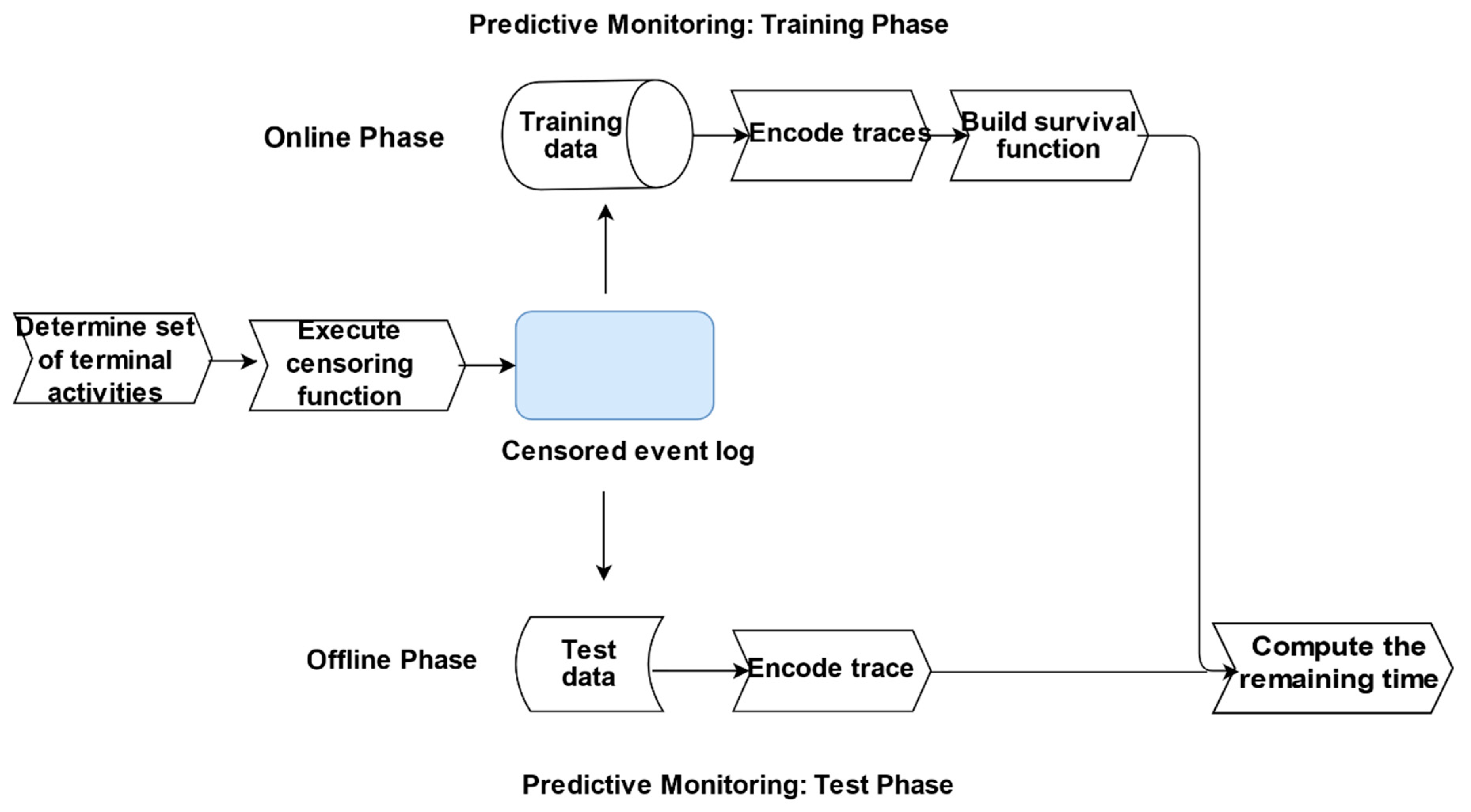
Figure 2 provides an overview of the proposed approach used in building and evaluating the predictive model (see Section 2.4). The initial step is the determination of the set of terminal activity labels which indicate the ‘successful’ completion of a trace. This set serves as input into the censoring function, which outputs a log where each trace is deemed censored or otherwise. We subsequently encode the log traces and build a survival model using the censored log. We recommend that these steps are performed offline to improve runtime performance.
Subsequently, in the offline phase, the remaining time for in-flight cases are predicted using the survival model.
2.3. Pre-Processing
To determine the set of terminal activity labels, we examine the process description and trace attributes of the respective datasets. However, in practice, this should be determined in conjunction with process subject matter experts. We utilise a function which examines whether the activity label associated with the terminal event for each trace, en (see Definition 2) is present within the set of terminal activity labels. If it is not, the trace is considered censored; otherwise, it is.
2.4. Predictive Monitoring
The approach consists of two phases: offline and online (see Figure 2). In the offline phase, the traces in the event log are encoded. We utilise a novel encoding approach, where we compute the grouped centrality measures for each trace (see Definition 11) using all the performers (#performer(e1)…. # performer(en)) associated with that trace as well as the start and end event activity labels. While we adopt that approach to explore the impact of social contextual factors on process cycle time, we acknowledge that other encoding approaches, such as index-based encoding which is “lossless” [9], could also be equally adopted. Our approach is in effect a combination of aggregation and last state encoding [14] where the aggregation function computes the group degree, betweenness, closeness, and eigenvalue centrality for each trace based on the set of performers who executed the events in that trace. This approach enables us to treat the performers who execute the activities in a trace as a team and builds on the approach in “the team effectiveness literature where researchers have used several internal team composition variables to predict performance” [21]. We utilise the parametric Weibull model to build the survival model. Even though it requires that certain assumptions regarding the distribution of the process cycle time are satisfied, this method offers several unique benefits in that it is “simultaneously both proportional and accelerated so that both relative event rates and relative extension in” process cycle “time can be estimated” [23].
In the online phase, the in-flight traces are encoded utilising the same approach as in the online phase. The survival model built in the offline phase is used to estimate the total cycle time for the trace, and the remaining time for the trace is computed by subtracting the elapsed time from the estimated cycle time.
Algorithm 1 details the survival analysis predictive modelling algorithm.
| Algorithm 1 Survival Algorithm. | |
| Input: | An event log L over some trace universe σ with the associated feature elapsed time τela, cycle time τcyc, a target measure remaining time τrem, a set of terminal activity labels (T), an estimation quantile q and a survival analysis (SURV) method |
| Output: | A Survival Analysis predictive model (SA-PM) for L |
| 1 | Associate a binary variable #censored(σ) with each trace σ ϵ L using #activity(en), T (see definition 3) |
| 2 | Encode each trace using a suitable encoding function |
| 3 | Induce a survival function sa-pm out of L using method SURV {#censored(σi), # cycle time(σi) …..# attributen(σi)} as input value |
| 4 | Let σ1… σn denote each trace |
| 5 | For each σi do |
| 6 | Estimate the cycle time τi.cyc_pred for each trace from sa-pm utilising q |
| 7 | Estimate the remaining time for each trace τi.rem_pred: τi.cyc_pred − τela |
| 8 | End |
| 9 | Return c {τrem_pred1……. τrem_predn} |
2.5. Evaluation
In this section, we perform two sets of experiments to address the research questions of interest in this study. In the first set of experiments, we evaluate the impact of social contextual features on the cycle time of process traces. In the second set of experiments, we evaluate the proposed survival analysis predictive monitoring techniques against similar predictive monitoring techniques. Specifically, we seek to address the following research questions:
RQ1: What is the relationship between social contextual factors and process completion time?
RQ2: How does the survival analysis predictive process monitoring approach compare with existing approaches?
In the following section, we provide further details about the experimental setup and how we answer the research questions.
2.5.1. Datasets
Five real-life event logs from the Business Process Intelligence Challenge (BPIC) were used for the experiments as follows: BPIC12 [24], BPIC14 [25], BPIC15(3) [26], BPIC17 [27], BPIC18 [28]. The logs were from a variety of domains covering diverse processes. To manage memory requirements, a subset of each event log (except for [24,26] where the entire log was used) was selected for the analysis. The event logs were selected on the basis that information about the performer (i.e., the individual resource or team) that executed each event (#performer (e)) is present in the log. This enabled us to create the social networks required to address the research questions. For example, [29] is not suitable as the resource attribute is abstracted to a high-level role (e.g., staff member). Moreover, basic feature engineering was performed to add required features such as elapsed time and remaining time to each log.
See Table 1 for a summary of the logs used for the experiments.
It is worth highlighting that, unlike the other logs, [25] had resources information at the team levels, so the handover of work was computed at a team rather than at an individual level.
2.5.2. Experimental Setup
As input into both sets of experiments, we created a social network from the handover of work from one performer to the next in each trace. We subsequently created an adjacency matrix and computed four grouped centrality measures—degree, betweenness, eigenvalue and closeness based on the approach recommended in [21]. In the initial sets of experiments, we performed some exploratory analysis by assigning each trace to a cluster using its four grouped centrality score. Before clustering the grouped centrality scores using a centroid-based clustering method (k-means), we empirically estimated the optimal numbers of clusters, k, from each dataset using the elbow method. We subsequently computed a survival curve for each cluster to visually determine how the grouped centrality scores impact the process cycle time. We subsequently created a case network to determine the relationship between these factors and case cycle times. We concluded by exploring the relationship between each group centrality measure and the cycle time.
For the second set of experiments, we implemented a survival analysis predictive monitoring approach named survival in R (as described in Section 2.4) which enables evaluation of this approach vis-à-vis similar existing approaches. The code and data for the experiments are located in the following GitHub repository (see https://github.com/etioro/SocialNetworks.git). We evaluated the survival analysis approach against two clustering-based remaining-time approaches identified in the literature (see [30,31]) and a couple of methods which used a zero prefix-bucketing combined with a gradient boosting machine (gbm) and multilayer perceptron (mlp) neural network regressors respectively to predict the remaining time for each trace [14]. The same set of features were used to build and evaluate all the models in the experiment.
We encode the traces as described in Section 2.4. Though this encoding is ‘lossy’, we adopt this approach as it enables us to capture the social contextual factors associated with each trace and adequately address the research questions
We split each event log into test and training sets (75:25 split, respectively), then used the training set to build the survival function and the test set for making remaining-time predictions, which are subsequently evaluated. As the survival curve gives a distribution of cycle time estimates, it was necessary to determine an optimal quantile for estimating the cycle time. We explored the approach suggested by [8,22] for selecting this quantile. This entails fitting a survival curve to the training set and determining which quantile minimised the MAE and RSME. This quantile is used to estimate the cycle time in the test set. However, we found that, compared to the median, this method performed poorly. Hence, we used the median as the optimal quantile for estimating the cycle time.
As with the methodology used in [14], the training and test set were not temporally disjoint.
We chose to utilise the mean absolute error (MAE) to evaluate the accuracy as other measures such as the root mean square error (RSME) are susceptible to outliers and mean percentage error (MAPE) would be skewed towards the end of a case where remaining time tends towards zero [9]. We filter the test set to use only non-censored traces to evaluate the MAE, as these are completed traces, whereas censored traces were abandoned or in-flight as at the time of log extraction.
3. Results
3.1. Experimental Results
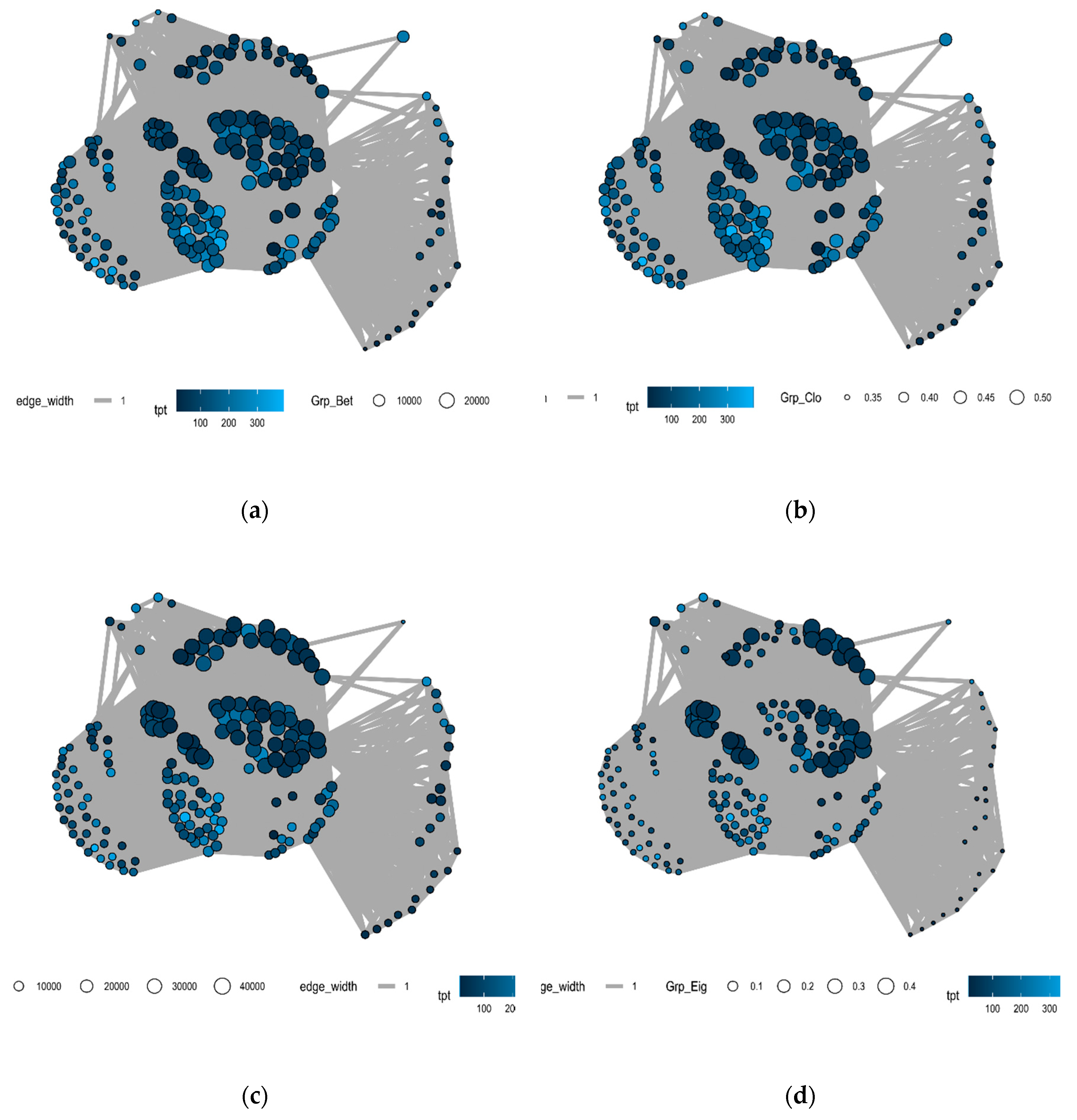
In the first set of experiments, to explore which of the group centrality factors have the most impact on the cycle, we created a network that visually illustrates the effect high and low values of the grouped centrality measures on case cycle times (see Figure 3a–d below). Each node represents a case, with cases which share common performers connected and the edges weighted by the number of shared performers. The size of the nodes is proportional to the relevant grouped centrality measure. The network appears to show an inverse relationship between cycle time and group degree and eigenvector centrality while the opposite is the case with the group closeness and betweenness centrality measures.
We explore these apparent relationships between the group centrality measures and trace cycle times further. Table 2 shows the Spearman rank correlation between each group centrality measure and the trace cycle time (with all the values statistically significant at the 95% confidence level in bold font). This test was selected to determine the strength and direction of the monotonic relationship between these measures. The group closeness centrality is the most strongly correlated measure to the trace cycle time, followed by the group eigenvector centrality. The group betweenness and closeness centrality were generally positively correlated while the group eigenvector centrality was generally negatively correlated.
We delve into the team effectiveness literature to sheds some light on these results. As [21] posits, “maintaining strong ties with people outside the team is an important determinant of team success”. We argue that these results may have implications for team setup as they shed light on the nature of these “ties”. For example, many organisations create specialised cells or SWAT teams to handle certain types of cases, e.g., complex cases. As a result, these teams could become isolated from other process performers which increases their probability of “failing” [32]. The results would seem to imply that connecting the teams to other influential performers in the organisation (high eigenvector centrality) will result in shorter cycle times, perhaps as a result of the ability of these performers to resolve issues relatively quickly. This would suggest that where such cells exist, it would be desirable to work cases with performers outside their cell periodically. Intuitively, this will increase the sharing of knowledge and experience across the organisation.
On the other hand, lower group betweenness across groups appears linked to lower cycle times. This measure is a proxy for how much the group is becoming a bottleneck across the organisation; perhaps because the performers are perceived as possessing certain desirable traits, e.g., viewed as experts or dependable. Lower group closeness centrality (a measure of the distance of the group to other performers) is also correlated with lower processing time as it indicates greater connectedness between performers.
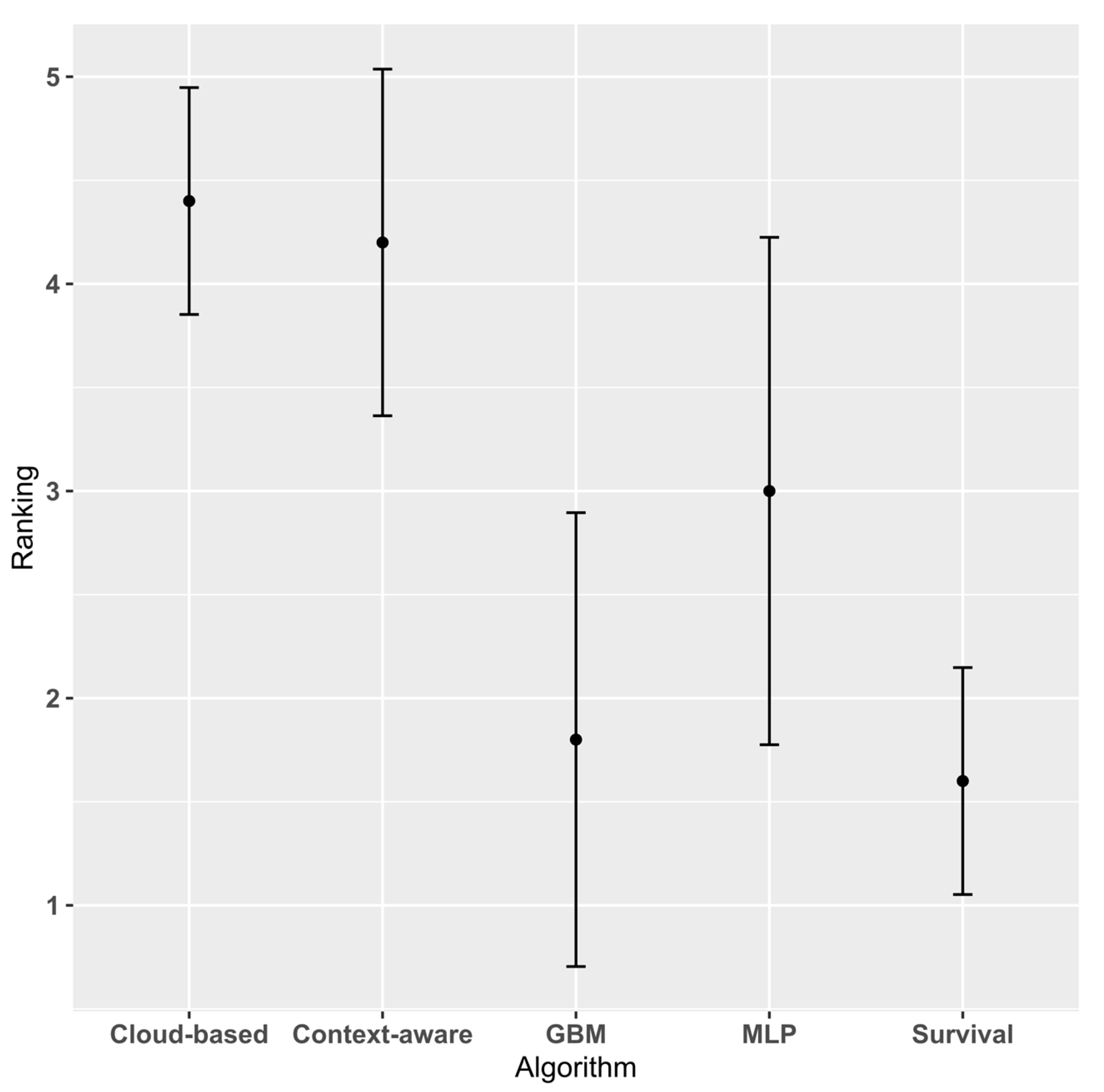
Progressing to the second set of experiments, Table 3 details the Global MAE and standard deviation (SD) for each dataset/algorithm pair. The performance of the algorithms is visualised in Figure 4, which displays the average ranking of each algorithm over the datasets with associated error bars. Over the five datasets, the survival analysis approach outperforms all the other approaches.
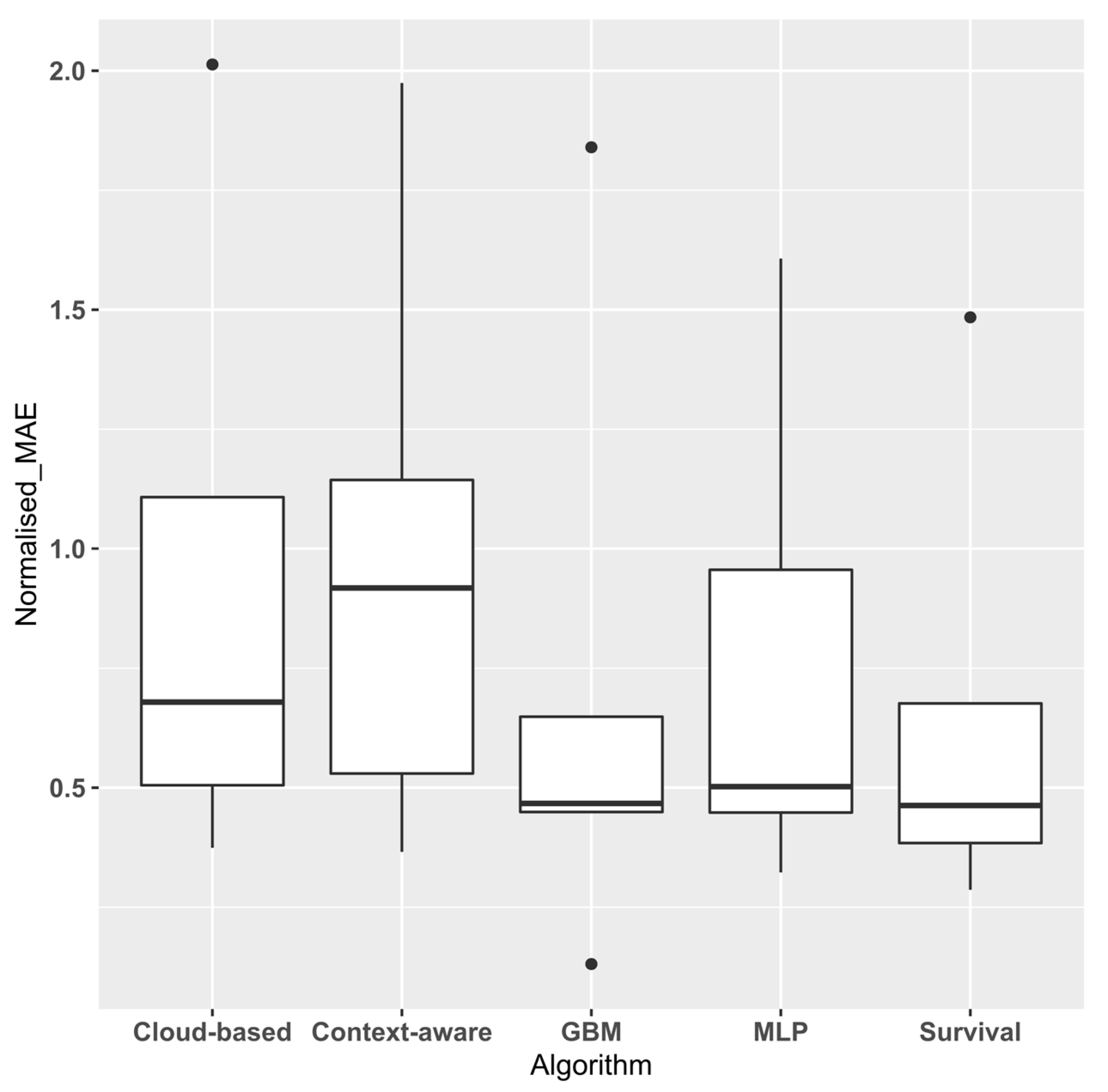
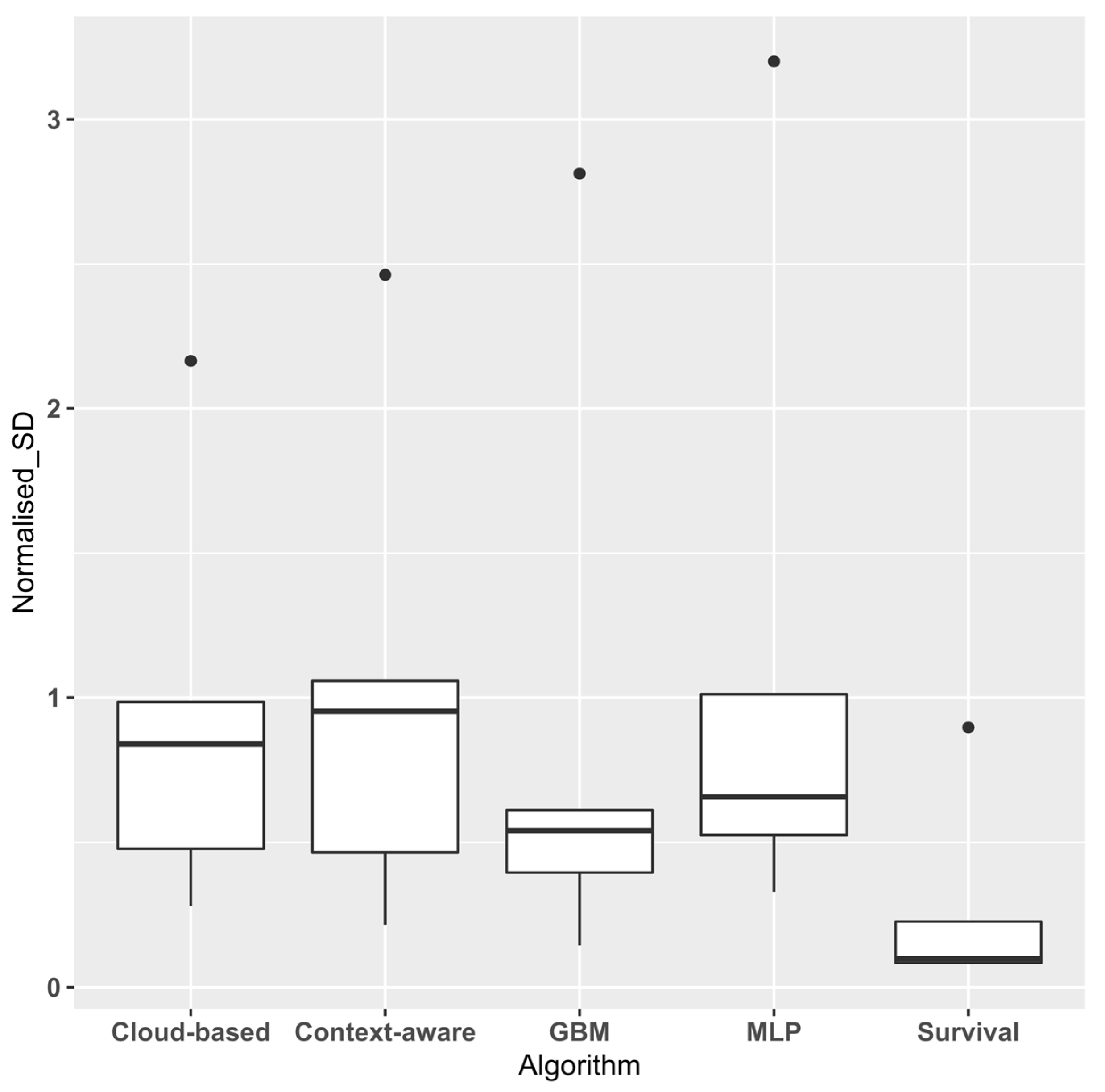
Figure 5 and Figure 6 show the aggregated error values obtained by dividing the Global MAE and SD by the average throughput time for each event log. Normalising these values enables them to be directly comparable [14]. The survival approach has the lowest normalised mean and median MAE (0.659 and 0.463, respectively), providing further confirmation of its superior performance.
As recommended by [33], the non-parametric Friedman test was performed on the ranked data to determine whether there was a significant difference between the algorithms. The test results indicate a statistically significant difference between the various algorithms at the 95% confidence level (p = 0.008687). To determine which algorithms differ from the others, we utilise the Quade post-hoc test to perform a pairwise comparison between the various algorithms. Table 4 shows the results of the pairwise comparisons (with all the values statistically significant at the 95% confidence level in bold font). The results indicate that the survival methods significantly outperformed all the existing methods except for gbm (see results in bold). To determine the explanation for this, we observe that event logs typically contain a portion of incomplete traces which are filtered out by existing approaches as they do not contribute any information towards accurately predicting the remaining time of the trace. Intuition supports this approach as we cannot determine whether an incomplete trace will finish in the next hour, day or year.
Ref. [14] provides a detailed discussion of generative and discriminative approaches for process monitoring. Discriminative approaches infer a conditional probability P(Y|X) from the training data set where X = ( …} denotes the set of feature variables and Y = {τrem_pred1, τrem_pred2….. τrem_predn} represents the prediction target. The resulting probability distribution is used to make predictions for the test set. However, when there is a significant proportion of incomplete traces in the training data, this approach is not useful as the target (Y), i.e., the remaining time for the trace, is unknown. This is the reason why these traces are typically removed from the training set. However, generative approaches, such as the survival analysis approach proposed, calculate a joint distribution P(X,Y) which is then utilised to derive the conditional probability P(Y|X). This approach can generate synthetic values of X by sampling from the joint distribution. As a result, this approach performs better when an event log has a significant proportion of incomplete trace.
In our experimental data, the percentage of incomplete traces ranged from 39% (BPIC 14) to 69% (BPIC 12). However, the survival analysis approach enables us to “account for (incomplete traces (i.e., censored data)) in the analysis” as this approach is able to extract information from them [34]. This is the main advantage of the approach we propose as it delivers better accuracy for event logs with a significant proportion of incomplete traces
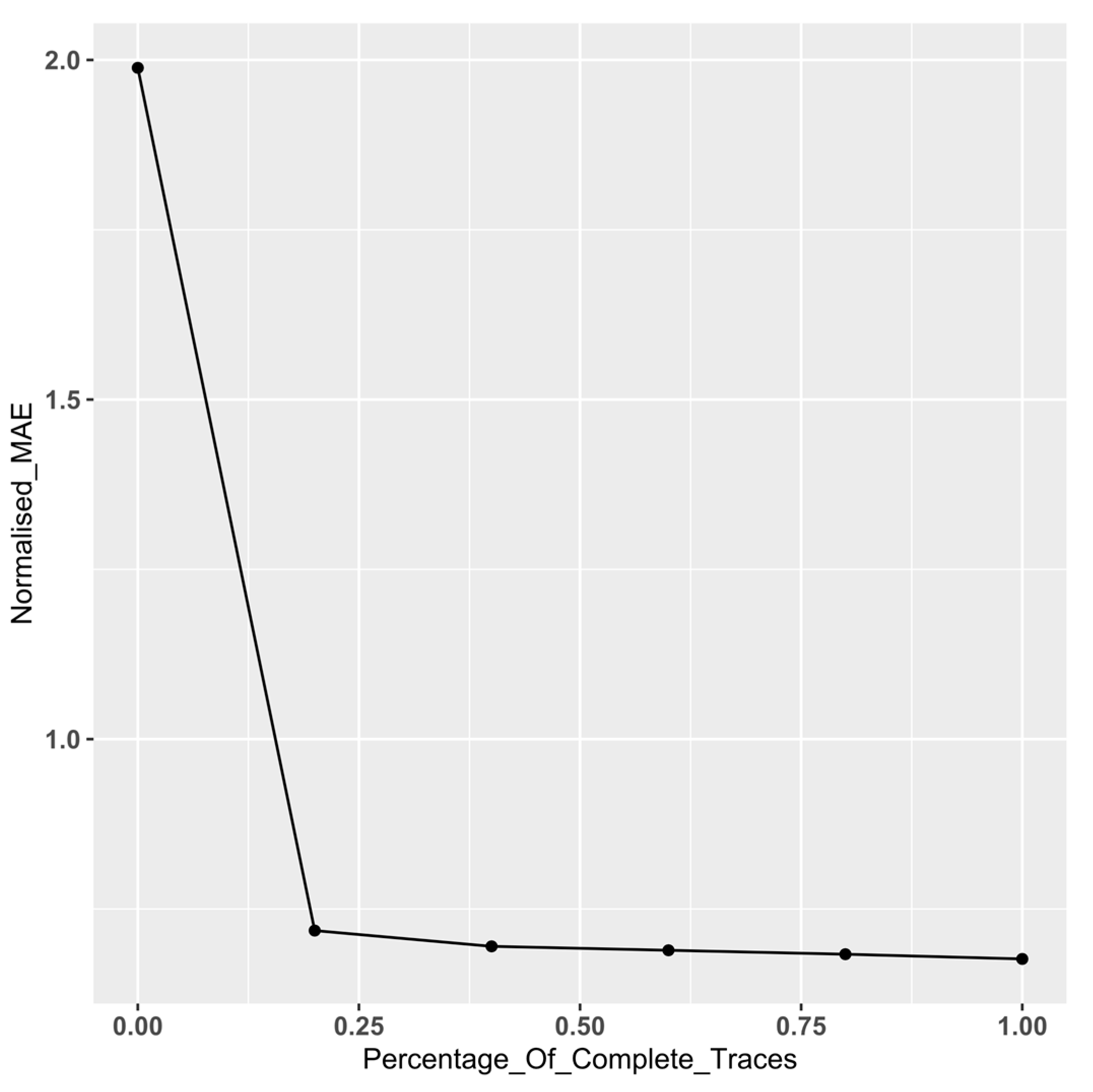
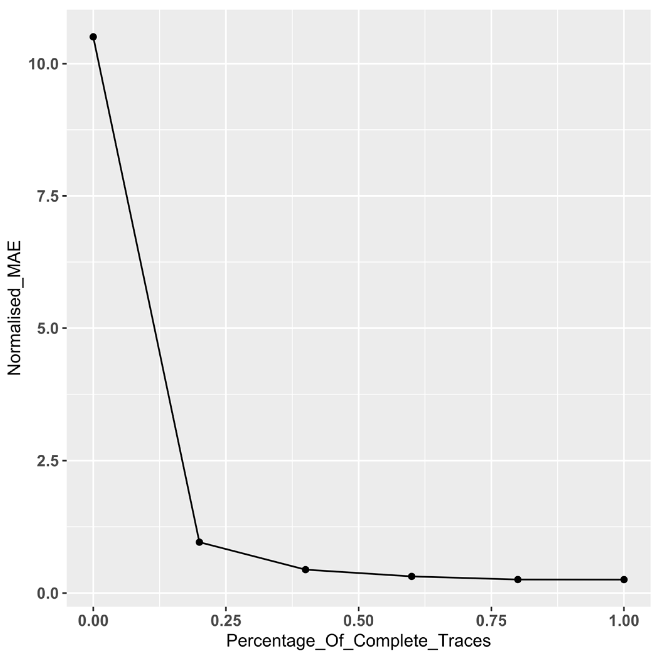
To explore the effect of the proportion of incomplete traces on performance, we perform an additional set of experiment utilising a subset of data from a couple of event logs (BPIC12 and BPIC18), selected as they are on opposite spectrums of event log complexity (see [1]). Keeping the size of the event log constant, we incrementally increase the percentage of incomplete traces in the log in steps of 20%, starting from 0% through to 100% (the baseline). We subsequently calculate the normalised MAE for each log using the proposed survival approach. Figure 7 and Figure 8 display the plots of the normalised MAE by the proportion of incomplete traces in the event log. As expected, both plots indicate a dramatic improvement in performance as the proportion of complete traces in the log increases. However, we observe that this improvement begins to level off once the proportion of complete traces exceeds c.60 %, after which the gain is less significant.
To test this effect, we utilise the non-parametric Kruskal–Wallis to determine whether there is a significant difference in the MAE for each log. As expected, there is a significant difference in the MAE for both logs (For BPIC 12, p = 3.282 × 10⁻⁹; for BPIC 18, p < 2.2 × 10⁻¹⁶). We subsequently run pairwise comparisons using Wilcoxon rank-sum test to determine which proportions differ significantly from the baseline (i.e., the log with 100% complete traces).
Table 5 shows the results of the pairwise comparisons against the baseline.
For BPIC 12, we notice that there is a significant difference until the point at which there is 40% incomplete traces (see results in bold). However, with BPIC 18, we notice that there is a significant difference between the MAE for all logs with incomplete traces against the baseline. To understand the results, we consider the event logs metrics (see Table 1). We observe that, despite having roughly the same number of events, BPIC 18 is more complex than BPIC 12 particularly in terms of mean trace length (×4) and the number of distinct activities (×6). We postulate that for complex event logs, our approach delivers a significant difference compared to the baseline, even when there is a high proportion of complete traces. However, for simpler logs, the difference is less pronounced, levelling out when there the proportion of complete cases approaches c.40%.
3.2. Threats to Validity
We encoded the traces using an aggregation encoding technique to enable us to address the research question regarding which social contextual factors were the most important. However, we acknowledge that this encoding technique is quite lossy, which may adversely impact prediction accuracy. As such, we would recommend combining this with other encoding approaches for real-life use.
The final threat to validity is related to the choice of grouped centrality measures selected as social contextual. We selected the most widely used centrality measures in the literature [18,21]. We, however, acknowledge that there are additional grouped centrality measures that we could have included (e.g., diffusion and fragmentation centrality) which may have shed further insight. We intend to explore the impact of these in future research studies.
4. Conclusions
This study has proposed an approach to censor an event log to facilitate its use for building a survival function. We explored the impact of social contextual factors as covariates in the survival function. We found that group betweenness and closeness centrality were generally positively correlated while the group eigenvector centrality was generally negatively correlated. We also found that survival analysis approaches perform comparably with start-of-the-art predictive process monitoring techniques.
In terms of further research, we propose a couple of areas for further exploration. Firstly, as an increasing number of automated agents augment the human workforce, we believe there is value in exploring how social networks between these categories of workers differ and the implications of these. Secondly, we propose an exploration of the effect the feature values of neighbouring nodes have on behaviour. For example, we could explore the temporal effect of a high workload on workers in an individual or group’s neighbourhood. This would enable a better understanding of workload distribution in the social network over time. In future work, we intend to attempt to tackle a number of these opportunities.
Author Contributions
Conceptualization, N.O.; methodology, N.O.; software, N.O. validation, A.B. and T.C.; formal analysis, N.O.; investigation, N.O.; resources, N.O., A.B. and T.C.; data curation, N.O.; writing—original draft preparation, N.O.; writing—review and editing, A.B. and T.C.; visualization, N.O.; supervision, A.B. and T.C.; project administration, N.O. All authors have read and agreed to the published version of the manuscript.
Funding
This research received no external funding.
Conflicts of Interest
The authors declare no conflict of interest.
References
- Van der Aalst, W.M. Process Mining: Data Science in Action, 2nd ed.; Springer: Berlin/Heidelberg, Germany, 2016. [Google Scholar]
- Tax, N.; Verenich, I.; La Rosa, M.; Dumas, M. Predictive business process monitoring with LSTM neural networks. In Proceedings of the International Conference on Advanced Information Systems Engineering, Essen, Germany, 12–16 June 2017; pp. 477–492. [Google Scholar]
- Aslan, A. Combining Process Mining and Queueing Theory for the ICT Ticket Resolution Process at LUMC. Master’s Thesis, University of Twente, Enschede, The Netherlands, 2017. [Google Scholar]
- Rogge-Solti, A.; Weske, M. Prediction of remaining service execution time using stochastic petri nets with arbitrary firing delays. In International Conference on Service-Oriented Computing; Springer: Berlin/Heidelberg, Germany, 2013; pp. 389–403. [Google Scholar]
- Akritas, M.G. Non-parametric survival analysis. Stat. Sci. 2004, 19, 615–623. [Google Scholar] [CrossRef] [Green Version]
- Somers, M.J. Modelling employee withdrawal behaviour over time: A study of turnover using survival analysis. J. Occup. Organ. Psychol. 1996, 69, 315–326. [Google Scholar] [CrossRef]
- Larivière, B.; Van den Poel, D. Investigating the role of product features in preventing customer churn, by using survival analysis and choice modeling: The case of financial services. Expert Syst. Appl. 2004, 27, 277–285. [Google Scholar] [CrossRef]
- Dirick, L.; Claeskens, G.; Baesens, B. Time to default in credit scoring using survival analysis: A benchmark study. J. Oper. Res. Soc. 2017, 68, 652–665. [Google Scholar] [CrossRef] [Green Version]
- Verenich, I.; Nguyen, H.; La Rosa, M.; Dumas, M. White-box prediction of process performance indicators via flow analysis. In Proceedings of the 2017 International Conference on Software and System Process Pages, ACM, Paris, France, 5–7 July 2017; pp. 85–94. [Google Scholar]
- Folino, F.; Guarascio, M.; Pontieri, L. Discovering Context-Aware Models for Predicting Business Process Performances. In On the Move to Meaningful Internet Systems, Proceedings of OTM 2012. OTM, Rome, Italy, 10–14 September 2012; Meersman, R., Panetto, H., Dillon, T., Rinderle-Ma, S., Dadam, P., Zhou, X., Pearson, S., Ferscha, A., Bergamaschi, S., Cruz, I.F., Eds.; Springer: Berlin/Heidelberg, Germany, 2012. [Google Scholar]
- Senderovich, A.; Di Francescomarino, C.; Ghidini, C.; Jorbina, K.; Maggi, F.M. ‘Intra and Inter-case Features in Predictive Process Monitoring: A Tale of Two Dimensions’. In Lecture Notes in Computer Science, Proceedings of Business Process Management. BPM 2017, Barcelona, Spain, 10–15 September 2017; Carmona, J., Engels, G., Kumar, A., Eds.; Springer: Cham, Switzerland, 2017; Volume 10445. [Google Scholar]
- Rozinat, A.; Wynn, M.T.; van der Aalst, W.M.; ter Hofstede, A.H.; Fidge, C.J. Workflow simulation for operational decision support. Data Knowl. Eng. 2009, 68, 834–850. [Google Scholar] [CrossRef]
- Veldhoen, J. The Applicability of Short-term Simulation of Business Processes for the Support of Operational Decisions. Master’s Thesis, Technische Universiteit Eindhoven, Eindhoven, The Newzerlands, March 2011. Available online: http://alexandria.tue.nl/extra2/afstversl/tm/Veldhoen%202011.pdf (accessed on 22 April 2020).
- Verenich, I.; Dumas, M.; La Rosa, M.; Maggi, F.M.; Teinemaa, I. Survey and Cross-Benchmark Comparison of Remaining Time Prediction Methods in Business Process Monitoring. Available online: https://arxiv.org/abs/1805.02896 (accessed on 11 May 2018).
- Breuker, D.; Matzner, M.; Delfmann, P.; Becker, J. Comprehensible Predictive Models for Business Processes. MIS Q. 2016, 40, 1009–1034. [Google Scholar] [CrossRef] [Green Version]
- Evermann, J.; Rehse, J.R.; Fettke, P. Predicting process behaviour using deep learning. Decis. Support Syst. 2017, 100, 129–140. [Google Scholar] [CrossRef] [Green Version]
- Pasquadibisceglie, V.; Appice, A.; Castellano, G.; Malerba, D. Using Convolutional Neural Networks for Predictive Process Analytics. In Proceedings of the 2019 International Conference on Process Mining (ICPM), Aachen, Germany, 24–26 June 2019; pp. 129–136. [Google Scholar]
- Van Der Aalst, W.M.; Reijers, H.A.; Song, M. Discovering social networks from event logs. Comput. Supported Coop. Work (CSCW) 2005, 14, 549–593. [Google Scholar] [CrossRef]
- Song, M.; Van der Aalst, W.M. Towards comprehensive support for organisational mining. Decis. Support Syst. 2008, 46, 300–317. [Google Scholar] [CrossRef] [Green Version]
- Nakatumba, J.; van der Aalst, W.M. Analysing resource behavior using process mining. In Proceedings of the International Conference on Business Process Management, Vienna, Austria, 1–6 September 2019; pp. 69–80. [Google Scholar]
- Everett, M.G.; Borgatti, S.P. The centrality of groups and classes. J. Math. Sociol. 1999, 23, 181–201. [Google Scholar] [CrossRef]
- Zhang, J.; Thomas, L.C. Comparisons of linear regression and survival analysis using single and mixture distributions approaches in modelling LGD. Int. J. Forecast. 2012, 28, 204–215. [Google Scholar] [CrossRef] [Green Version]
- Carroll, K.J. On the use and utility of the Weibull model in the analysis of survival data. Control. Clin. Trials 2003, 24, 682–701. [Google Scholar] [CrossRef]
- van Dongen, B.F. BPI Challenge 2012. 4TU. Centre for Research Data. Dataset. Available online: https://data.4tu.nl/articles/BPI_Challenge_2012/12689204 (accessed on 4 May 2020).
- van Dongen, B.F. BPI Challenge 2014. 4TU. Centre for Research Data. Dataset. Available online: https://data.4tu.nl/collections/BPI_Challenge_2014/5065469 (accessed on 4 May 2020).
- van Dongen, B.F. BPI Challenge 2015 Municipality 3. Eindhoven University of Technology. Dataset. Available online: https://data.4tu.nl/articles/dataset/BPI_Challenge_2015_Municipality_3/12718370 (accessed on 4 May 2020).
- van Dongen, B.F. BPI Challenge 2017. Eindhoven University of Technology. Dataset. Available online: https://data.4tu.nl/articles/BPI_Challenge_2017/12696884 (accessed on 4 May 2020).
- van Dongen, B.F. BPI Challenge 2018. Eindhoven University of Technology. Dataset. Available online: https://data.4tu.nl/articles/BPI_Challenge_2018/12688355 (accessed on 4 May 2020).
- van Dongen, B.F. BPI Challenge 2020. 4TU. Centre for Research Data. Dataset. 2020. Available online: https://data.4tu.nl/collections/BPI_Challenge_2020/5065541 (accessed on 26 May 2020).
- Bevacqua, A.; Carnuccio, M.; Folino, F.; Guarascio, M.; Pontieri, L. A Data-Driven Prediction Framework for Analysing and Monitoring Business Process Performances. In Lecture Notes in Business Information Processing, Proceedings of Enterprise Information Systems. ICEIS 2013, Angers, France, 4–7 July 2013; Hammoudi, S., Cordeiro, J., Maciaszek, L., Filipe, J., Eds.; Springer: Cham, Switzerland, 2014; Volume 190. [Google Scholar]
- Cesario, E.; Folino, F.; Guarascio, M.; Pontieri, L. A Cloud-Based Prediction Framework for Analyzing Business Process Performances; Springer: Cham, Switzerland, 2016. [Google Scholar]
- Ancona, D.G. Outward bound: Strategic for team survival in an organization. Acad. Manag. J. 1990, 33, 334–365. [Google Scholar] [CrossRef]
- Demšar, J. Statistical comparisons of classifiers over multiple data sets. J. Mach. Learn. Res. 2006, 7, 1–30. [Google Scholar]
- Linden, A.; Yarnold, P.R. Modeling time-to-event (survival) data using classification tree analysis. J. Eval. Clin. Pract. 2017, 23, 1299–1308. [Google Scholar] [CrossRef] [PubMed]
Figure 1.
Contextual Factors and Relationship—(Adapted from [1]).
Figure 1.
Contextual Factors and Relationship—(Adapted from [1]).

Figure 2.
Overview of the proposed approach.

Figure 3.
(a) BPIC 14 Group Between Centrality Graph; (b) BPIC 14 Group Closeness Centrality Graph; (c) BPIC 14 Group Degree Centrality Graph; (d) BPIC 14 Group Eigenvalue Centrality Graph.
Figure 3.
(a) BPIC 14 Group Between Centrality Graph; (b) BPIC 14 Group Closeness Centrality Graph; (c) BPIC 14 Group Degree Centrality Graph; (d) BPIC 14 Group Eigenvalue Centrality Graph.

Figure 4.
Average Algorithm Ranking with associated error bars.

Figure 5.
Average Normalised MAE.

Figure 6.
Average Normalised Standard Deviation.

Figure 7.
BPIC 12—Normalised MAE by proportion of incomplete traces.

Figure 8.
BPIC 18—Normalised MAE by proportion of incomplete traces.


Table 1.
Event Log Overview.
| BPIC 18 | BPIC 17 | BPIC 15(3) | BPIC 14 | BPIC 12 | |
|---|---|---|---|---|---|
| Number of events | 267,830 | 233,928 | 59,681 | 277,577 | 262,200 |
| Number of cases | 3285 | 9453 | 1409 | 13,985 | 13,087 |
| Number of traces | 3277 | 5211 | 1350 | 13,942 | 4366 |
| Number of distinct activities | 141 | 26 | 277 | 39 | 24 |
| Mean trace length | 81.53 | 24.75 | 42.36 | 19.85 | 20.04 |
| Mean throughput time (days) | 580.63 | 24.11 | 62.23 | 12.93 | 8.62 |
| Throughput time SD (days) | 580.62 | 14.893 | 97.64 | 27.94 | 12.13 |
| Domain | Public Admin | Financial services | Public Admin | Financial services | Financial services |
Table 2.
Spearman Rank Correlation between group centrality measure and trace cycle time.
| GB | GC | GE | GD | |
|---|---|---|---|---|
| BPIC 18 | −0.058 | −0.014 | 0.248 | 0.107 |
| BPIC 17 | 0.063 | 0.176 | 0.063 | 0.093 |
| BPIC 15(3) | 0.289 | 0.414 | −0.208 | −0.045 |
| BPIC 14 | 0.078 | 0.119 | −0.183 | −0.171 |
| BPIC 12 | 0.877 | 0.848 | −0.475 | −0.003 |
Table 3.
Global Mean Average Error ± Standard Deviation.
| Survival | MLP | GBM | Cloud-Based | Context-Aware | |
|---|---|---|---|---|---|
| BPIC 18 | 166.27 ± 46.6 | 187.37 ± 190.62 | 76.09 ± 84.18 | 217.27 ± 162.30 | 212.34 ± 124.37 |
| BPIC 17 | 11.158 ± 2.03 | 12.11 ± 12.67 | 10.83 ± 9.54 | 12.18 ± 11.53 | 12.77 ± 11.23 |
| BPIC 15(3) | 23.91 ± 6.12 | 27.88 ± 40.91 | 29.07 ± 33.63 | 42.26 ± 52.27 | 57.12 ± 59.31 |
| BPIC 14 | 19.19 ± 11.6 | 20.78 ± 41.39 | 23.79 ± 36.37 | 26.03 ± 27.99 | 25.53 ± 31.84 |
| BPIC 12 | 5.83 ± 1.95 | 8.24 ± 8.72 | 5.59 ± 5.27 | 9.55 ± 8.49 | 9.86 ± 9.12 |
Table 4.
Pairwise comparisons using posthoc-Quade test.
| Survival | MLP | GBM | Cloud-Based | |
|---|---|---|---|---|
| MLP | 0.04173 | |||
| GBM | 0.75592 | 0.07598 | ||
| Cloud-based | 0.00042 | 0.04173 | 0.00082 | |
| Context-aware | 0.00082 | 0.07598 | 0.00159 | 0.75592 |
Table 5.
Pairwise Comparisons against the baseline using Wilcoxon rank-sum test.
| % of Complete Traces in Event Log | |||||
|---|---|---|---|---|---|
| 0% | 20% | 40% | 60% | 80% | |
| BPIC 12 | 1.2 × 10⁻⁷ | 0.0003 | 0.1158 | 0.0737 | 0.0909 |
| BPIC 18 | <2 × 10⁻¹⁶ | <2 × 10⁻¹⁶ | <2 × 10⁻¹⁶ | 2.5 × 10⁻¹⁶ | 6.0 × 10⁻¹² |
Publisher’s Note: MDPI stays neutral with regard to jurisdictional claims in published maps and institutional affiliations. |
© 2020 by the authors. Licensee MDPI, Basel, Switzerland. This article is an open access article distributed under the terms and conditions of the Creative Commons Attribution (CC BY) license (http://creativecommons.org/licenses/by/4.0/).
Share and Cite
MDPI and ACS Style
Ogunbiyi, N.; Basukoski, A.; Chaussalet, T. Investigating Social Contextual Factors in Remaining-Time Predictive Process Monitoring—A Survival Analysis Approach. Algorithms 2020, 13, 267. https://0-doi-org.brum.beds.ac.uk/10.3390/a13110267
AMA Style
Ogunbiyi N, Basukoski A, Chaussalet T. Investigating Social Contextual Factors in Remaining-Time Predictive Process Monitoring—A Survival Analysis Approach. Algorithms. 2020; 13(11):267. https://0-doi-org.brum.beds.ac.uk/10.3390/a13110267
Chicago/Turabian StyleOgunbiyi, Niyi, Artie Basukoski, and Thierry Chaussalet. 2020. "Investigating Social Contextual Factors in Remaining-Time Predictive Process Monitoring—A Survival Analysis Approach" Algorithms 13, no. 11: 267. https://0-doi-org.brum.beds.ac.uk/10.3390/a13110267
Note that from the first issue of 2016, this journal uses article numbers instead of page numbers. See further details here.