Translating Workflow Nets to Process Trees: An Algorithmic Approach

Abstract

Since their introduction, process trees have been frequently used as a process modeling formalism in many process mining algorithms. A process tree is a (mathematical) tree-based model of a process, in which internal vertices represent behavioral control-flow relations and leaves represent process activities. Translation of a process tree into a sound workflow net is trivial. However, the reverse is not the case. Simultaneously, an algorithm that translates a WF-net into a process tree is of great interest, e.g., the explicit knowledge of the control-flow hierarchy in a WF-net allows one to reason on its behavior more easily. Hence, in this paper, we present such an algorithm, i.e., it detects whether a WF-net corresponds to a process tree, and, if so, constructs it. We prove that, if the algorithm finds a process tree, the language of the process tree is equal to the language of the original WF-net. The experiments conducted show that the algorithm’s corresponding implementation has a quadratic time complexity in the size of the WF-net. Furthermore, the experiments show strong evidence of process tree rediscoverability.

1. Introduction

Process mining [1] is concerned with distilling knowledge of the execution of processes by analyzing the event data generated during the execution of these processes, i.e., stored in modern-day information systems. In the field, different (semi-)automated techniques have been developed that allow one to distill knowledge of a process from event data, ranging from automated process discovery algorithms to conformance checking algorithms. In automated process discovery, the main aim is to translate observed process behavior, i.e., as stored in the information system, into a process model that accurately describes the behavior of the process. In this context, the discovered process model should strike an adequate balance between accounting for unobserved, yet likely, process behavior (i.e., avoiding overfitting) and being precise (i.e., avoiding underfitting) at the same time. Conformance checking techniques allow us to compute to what degree the observed behavior is in line with a given reference process model (either designed by hand or discovered using an automated process discovery technique). Since processes are the cornerstone of process mining, so are the models that allow us to represent them (and reason about their behavior and quality). As such, various process modeling formalisms exist, e.g., BPMN [2], EPCs [3], etc., some of which are heavily used in practice.

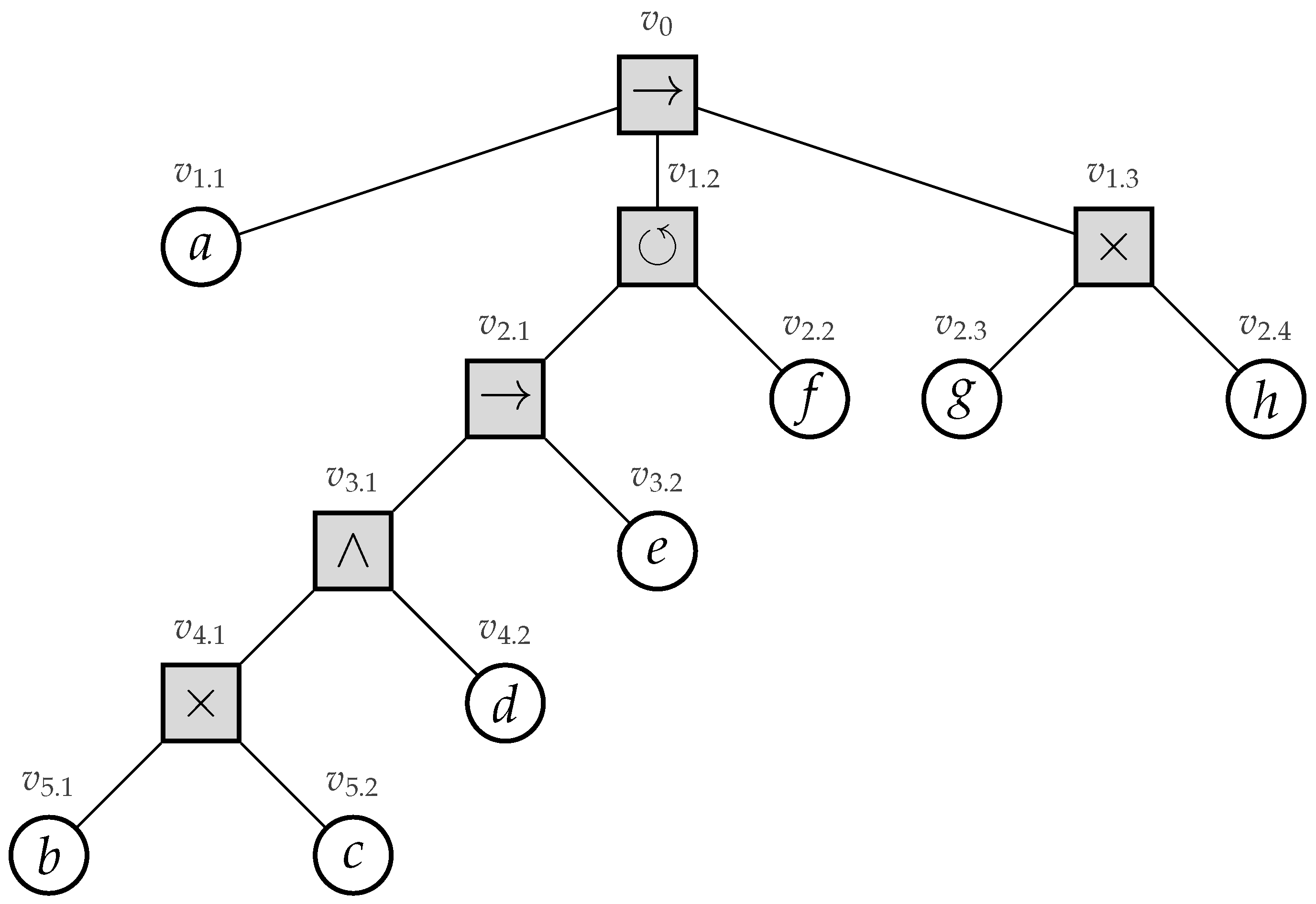
Recently, process trees were introduced [4]. A process tree is a hierarchical representation of a process corresponding to the mathematical notion of a rooted tree, i.e., a connected undirected acyclic graph with a designated root vertex. The internal vertices of a process tree represent how their children relate to each other regarding their control-flow behavior (i.e., their sequential scheduling). The leaves of the tree represent the activities of the process. Consider Figure 1, in which we depict an example process tree.

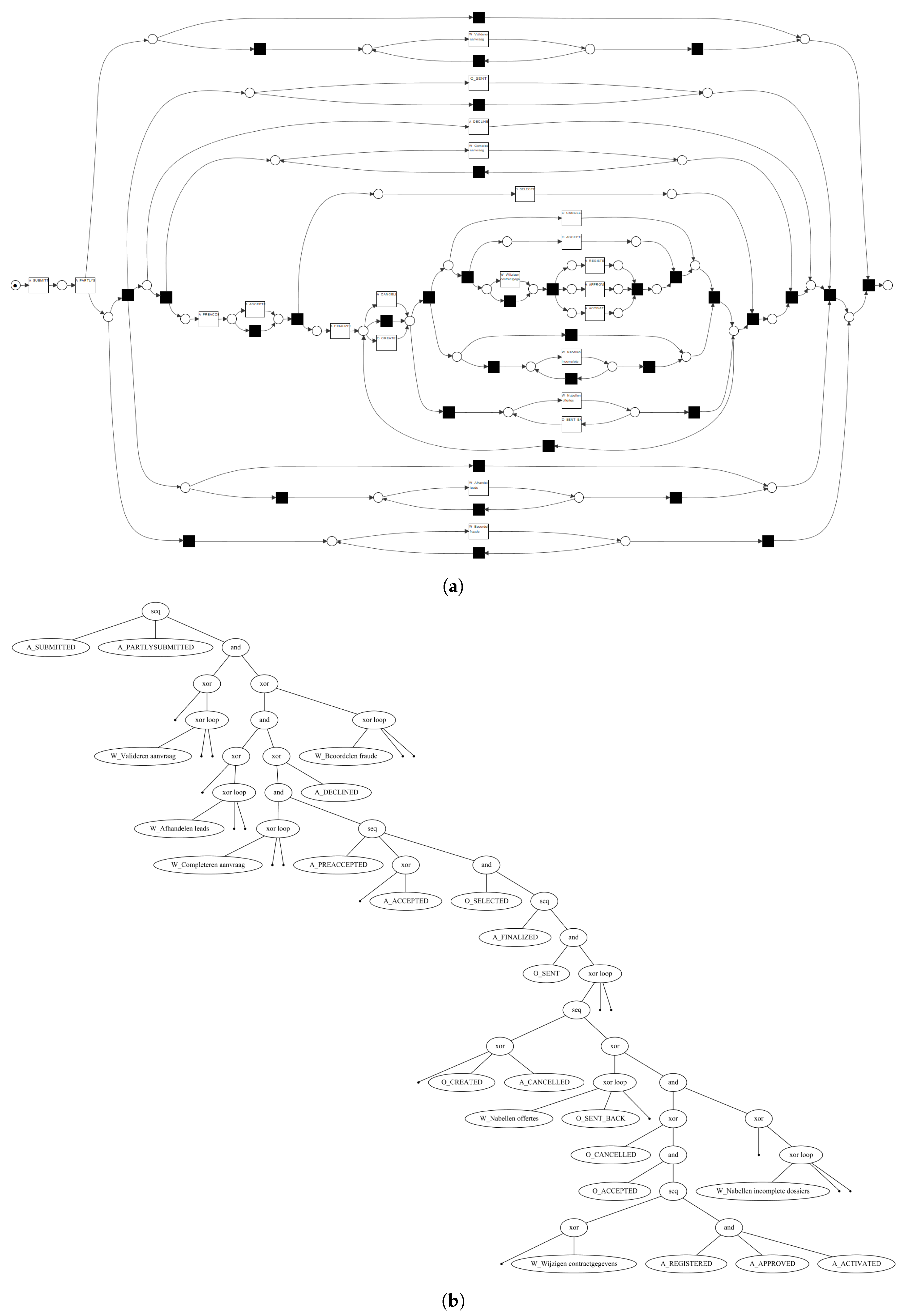
Its root vertex has label →, specifying that first its leftmost child, i.e., activity a, needs to be executed, secondly its middle child, and, finally, its rightmost child. Its middle child has a ⥀ label, specifying cyclic behavior, i.e., its leftmost child is always executed, whereas the execution of its rightmost child stipulates that we need to repeat its leftmost child. The ×-label in a process tree represents an exclusive choice, e.g., vertex $v_{1.3}$ specifies that we either executed activity g or h, yet not both. Finally, the ∧-label refers to concurrency, i.e, the children of a vertex with such a label are allowed to be executed simultaneously, i.e., at the same time. Furthermore, consider the two models depicted in Figure 2 (page 3), i.e., a Workflow net (WF-net) and a process tree (note that the activity labels within the model are not depicted in a readable fashion, i.e., the main aim of the figure is to illustrate the structural differences between WF-nets and process trees). The models represent the same behavior, based on a real-life event log. Clearly, the hierarchy of the process tree allows one to more easily understand the main control-flow of the process.

The previous examples show the relative simplicity at which one can reason on the behavior of a process tree. Furthermore, it is straightforward to translate process trees into other process modeling formalisms, e.g., WF-nets, BPMN models, etc. By definition, a process tree corresponds to a sound WF-net, i.e., a WF-net with desirable behavioral properties, e.g., the absence of deadlocks. The reverse, i.e., translating a given WF-net into a process tree (if possible), is less trivial. At the same time, obtaining such a translation is of great interest, e.g., it allows us to discover control-flow-aware hierarchical structures within a WF-net. Such structures can, for example, be used to hide certain parts of the model, i.e., leading to a more understandable view of the process model. Furthermore, any algorithm optimized for process trees, e.g., by exploiting the hierarchical structure, can also be applied to WF-nets of such a type. For example, in [5], it is shown that the computation time of alignments [6], i.e., explanations of observed behavior in terms of a reference model, can be significantly reduced by applying Petri net decomposition on the basis of model hierarchies. Hence, computing a process tree representation of the WF-net can be exploited to reduce the computational complexity of the calculations mentioned. Furthermore, recently, an alignment approximation technique was proposed that explicitly exploits the tree structure of a process tree [7]. Additionally, computing the underlying canonical process tree structure of two different process models allows us to decide whether or not the two models are behaviorally equivalent, e.g., as studied in [8,9]. In a similar fashion, the process tree representation of a workflow net can be exploited to translate it to a different process modeling formalism, i.e., known as process model transformation [10].

In this paper, we present an algorithm that determines whether a given WF-net corresponds to a process tree, and, if so, constructs it. We prove that, if the algorithm finds a process tree, the original WF-net is sound, and the obtained process tree’s language is equal to the language of the original WF-net. A corresponding implementation, extending the process mining framework PM4Py [11], is publicly available. Using the implementation, we conducted several experiments that show a quadratic time complexity in terms of the WF-net size. Furthermore, our experiments indicate that the algorithm can rediscover process trees, i.e., the process models used to generate the input for the experiments are rediscovered by the algorithm.

The remainder of this paper is structured as follows. In Section 2, we present preliminary concepts and notation. In Section 3, we present the proposed algorithm, including the proofs with respect to soundness preservation and language preservation. In Section 4, we evaluate our approach. In Section 5, we discuss related work. In Section 6, we discuss various aspects of our approach, e.g., extensibility, in more detail. Section 7 concludes the paper.

2. Preliminaries

In this section, we present basic preliminary notions that ease the readability of this paper. In Section 2.1, we present the basic notation used in this paper. In Section 2.2, we introduce Workflow nets. Finally, in Section 2.3, we present the notion of process trees and their relation to Workflow nets.

2.1. Basic Notation

Given set X, $\mathcal{P}(X)=\left\{X^{\prime }\subseteq X\right\}$ denotes its powerset. Given a function $f:X\to Y$ and $X^{\prime }\subseteq X$, we extend function application to sets, i.e., $f(X^{\prime })=\{y\mid \exists x\in X^{\prime }(f(x)=y)\}$. Furthermore, ${f|}_{X^{\prime }}:X^{\prime }\to Y$ restricts f to $X^{\prime }$. A multiset over set X, i.e., $m:X\to \mathbb{N}\cup \{0\}$, contains multiple instances of an element. We write a multiset as $m=[x_1^i,x_2^j,\dots ,x_n^k]$, where $m(x_1)=i,m(x_2)=j,\dots ,m(x_n)=k$, for $i,j,\dots ,k>1$ (in case, $m(x_i)=1$, we omit its superscript; in case $m(x_i)=0$, we omit $x_i$). The set of all multisets over X is written as $\mathcal{M}(X)$. Given $m\in \mathcal{M}(X)$, we write $x{\in }_{+}m$ if $m(x)>0$, and, $x{\notin }_{+}m$ if $m(x)=0$, and, $\overline{m}=\{x|x{\in }_{+}m\}$. For example, the multiset $[x^2,y]$ consists of two instances of x, one instance of y, and zero instances of z. The sum of two multisets $m_1,m_2$ is written as $m_1\uplus m_2$, e.g., $[x^2,y]\uplus [x^3,y,z]=[x^5,y^2,z]$, and their difference is written as $m_1-m_2$, e.g., $[x^2,y]-[x,y,z]=[x]$. A set is considered a multiset in which each element appears only once. Hence, we also apply the operations defined for multisets on sets, and, on combinations of sets and multisets, e.g., $\{x,y,z\}\uplus [x^2]=[x^3,y,z]$.

A sequence is an ordered collection of elements, e.g., a sequence $\sigma$ of length n over base set X is a function $\sigma :\{1,\dots ,n\}\to X$. We write $\left|\sigma \right|$ to denote the length of $\sigma$, e.g., $\left|\sigma \right|=n$. We write $\sigma =\langle \sigma (1),\sigma (2),\dots ,\sigma (|\sigma |)\rangle$, where $\sigma (i)$ denotes the element at position i, ($1\le i\le \left|\sigma \right|$). $ϵ$ denotes the empty sequence, i.e., $\left|ϵ\right|=0$. We extend the notion of element inclusion to sequences, e.g., $x\in \langle x,y,z\rangle$. $X^{*}$ denotes the set of all sequences over members of set X. Concatenation of sequences $\sigma ,{\sigma }^{\prime }\in X^{*}$ is written as $\sigma ·{\sigma }^{\prime }$. We let $\sigma \leftrightharpoons {\sigma }^{\prime }$ denote the set of all possible order-preserving merges, i.e., the shuffle operator, of $\sigma$ and ${\sigma }^{\prime }$, e.g., given ${\sigma }_1=\langle b,p\rangle$, ${\sigma }_2=\langle m\rangle$, then ${\sigma }_1\leftrightharpoons {\sigma }_2=\left\{\langle b,p,m\rangle ,\langle b,m,p\rangle ,\langle m,b,p\rangle \right\}$. It is easy to see that $\sigma \leftrightharpoons {\sigma }^{\prime }={\sigma }^{\prime }\leftrightharpoons \sigma$ (the operator is commutative). We extend the shuffle operator to sets (and overload notation), i.e., given $S,S^{\prime }\in X^{*}$, $S\leftrightharpoons S^{\prime }=\{\sigma \in {\sigma }_1\leftrightharpoons {\sigma }_2\mid {\sigma }_1\in S_1\wedge {\sigma }_2\in S_2\}$. Note that $(\sigma \leftrightharpoons {\sigma }^{\prime })\leftrightharpoons \{{\sigma }^{\prime \prime }\}=\{\sigma \}\leftrightharpoons ({\sigma }^{\prime }\leftrightharpoons {\sigma }^{\prime \prime })$ (associative); hence, we write the application of the shuffle operation on n sequences as ${\sigma }_1\leftrightharpoons {\sigma }_2\leftrightharpoons \cdots \leftrightharpoons {\sigma }_n$. Similarly, we write $S_1\leftrightharpoons S_2\leftrightharpoons \cdots \leftrightharpoons S_n$ for sets of sequences $S_1,S_2,\dots S_n\in X^{*}$. Given a function $f:X\to Y$ and a sequence $\sigma \in X^{*}$, we overload notation for function application, i.e., $f(\sigma )=\langle f(\sigma (1),f(\sigma (2)),\dots ,f(\sigma \left|\sigma \right|)\rangle$. We extend the notion of sequence application to sets of sequences, i.e., given $f:X\to Y$ and $X^{\prime }\subseteq X^{*}$, $f(X^{\prime })=\{\sigma \in Y^{*}\mid \exists {\sigma }^{\prime }\in X^{\prime }\left(f({\sigma }^{\prime })=\sigma \right)\}$. Furthermore, given $X^{\prime }\subseteq X$ and a sequence $\sigma \in X^{*}$, we define ${\sigma }_{{\downarrow }_{X^{\prime }}}$, where (recursively) ${ϵ}_{{\downarrow }_{X^{\prime }}}=ϵ$, ${(\langle x\rangle ·\sigma )}_{{\downarrow }_{X^{\prime }}}=x·{\sigma }_{{\downarrow }_{X^{\prime }}}$ if $x\in X^{\prime }$ and ${(\langle x\rangle ·\sigma )}_{{\downarrow }_{X^{\prime }}}={\sigma }_{{\downarrow }_{X^{\prime }}}$ if $x\notin X^{\prime }$.

2.2. Workflow Nets

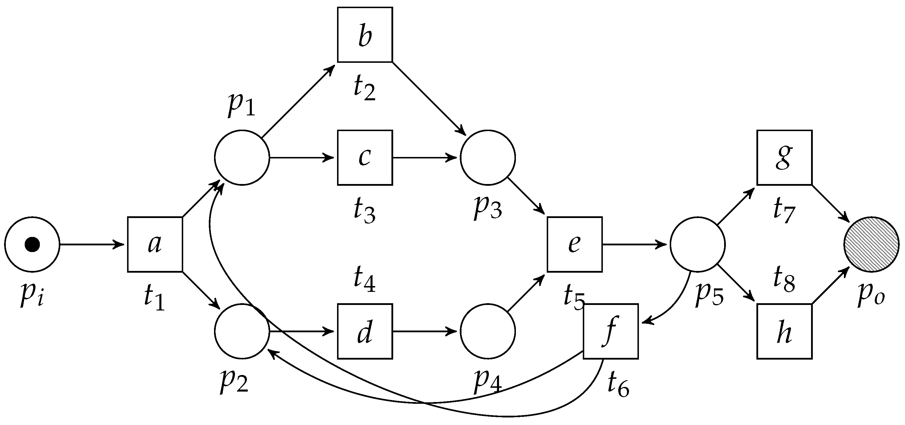
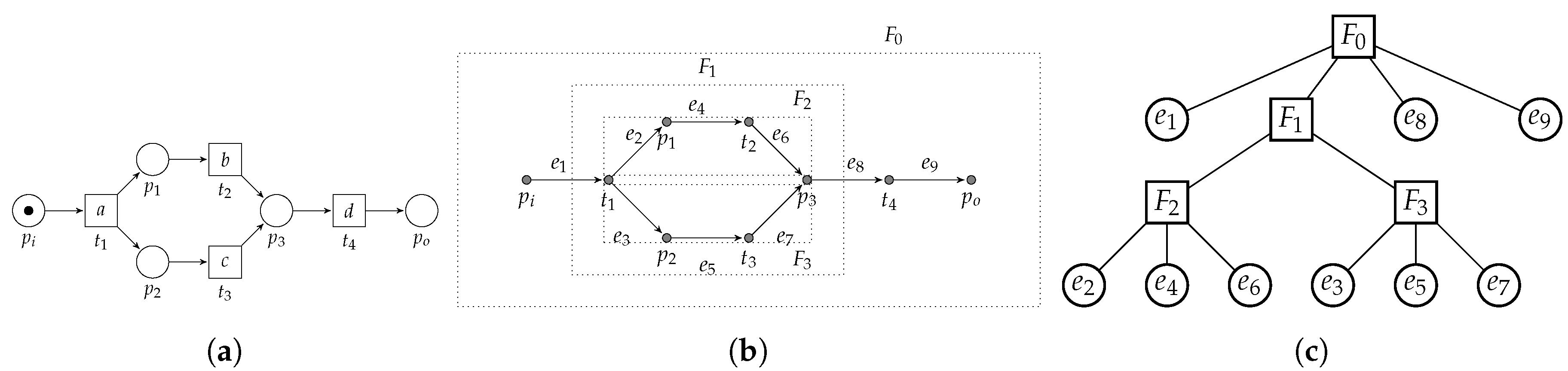
Workflow nets (WF-nets) [15] extend the more general notion of Petri nets [16]. A Petri net is a directed bipartite graph containing two types of vertices, i.e., places and transitions. We visualize places as circles, whereas we visualize transitions as boxes. Places only connect to transitions and vice versa. Consider Figure 3, depicting an example Petri net (which is also a WF-net). We let $N=(P,T,F,\ell )$ denote a labeled Petri net, where, P denotes a set of places, T denotes a set of transitions and $F\subseteq (P\times T)\cup (T\times P)$ represents the arcs. Furthermore, given a set of labels $\Sigma$ and the symbol $\tau \notin \Sigma$, $\ell :T\to \Sigma \cup \{\tau \}$ is the net’s labelling function, e.g., in Figure 3, $\ell (t_1)=a$, $\ell (t_2)=b$, etc. Given an element $x\in P\cup T$, $•x=\left\{y\mid (y,x)\in F\right\}$ denotes the pre-set of x, whereas $x•=\left\{y|(x,y)\in F\right\}$ denotes its post-set, e.g., in Figure 3, $•t_1=\left\{p_i\right\}$ and $p_1•=\left\{t_2,t_3\right\}$. We lift the •-notation to the level of sets, i.e., given $X\subseteq P\cup T$, $•X=\left\{y\mid \exists x\in X\left(y\in •x\right)\right\}$ and $X•=\left\{y\mid \exists x\in X\left(y\in x•\right)\right\}$. Let $N=(P,T,F,\ell )$ be a Petri net and let $P^{\prime }\subseteq P$, $T^{\prime }\subseteq T$ and $F^{\prime }=F\cap ((P^{\prime }\times T^{\prime })\cup (T^{\prime }\times P^{\prime }))$. The Petri net $N^{\prime }=\left(P^{\prime },T^{\prime },F^{\prime }{,\ell |}_{T^{\prime }}\right)$ is a subnet of N, written $N^{\prime }⊑N$. In the context of this paper, we refer to a subnet $N^{\prime }⊑N$ as a fragment if it is weakly connected. Furthermore, a fragment $N^{\prime }⊑N$ is place-bordered iff the only vertices of $N^{\prime }$ (i.e., members of $P^{\prime }\cup T^{\prime }$) that are connected to vertices that do not belong to $N^{\prime }$ (i.e., members of $P\cup T\backslash (P^{\prime }\cup T^{\prime })$) are places, i.e., $\{x\in P^{\prime }\cup T^{\prime }\mid (x,y)\in F\backslash F^{\prime }\vee (y,x)\in F\backslash F^{\prime }\}\subseteq P^{\prime }$. Furthermore, we refer to $P_i^{\prime }=\{x\in P^{\prime }\mid (y,x)\in F\backslash F^{\prime }\}$ and $P_o^{\prime }=\{x\in P^{\prime }\mid (x,y)\in F\backslash F^{\prime }\}$ to the input and output places of the place-bordered fragment. For example, in Figure 3, the subnet formed by places $p_1$, $p_2$, $p_3$, $p_4$, $p_5$, transitions $t_2$, $t_3$, $t_4$, $t_5$ and the arcs $(p_1,t_2),(p_1,t_3),\dots ,(t_5,p_5)$ is a place-bordered fragment. Observe that, if we remove place $p_5$ (and the corresponding arc $(t_5,p_5)$), the subnet is still a fragment, yet, no longer place-bordered. If we also remove $t_5$ and the arcs $(p_3,t_5)$ and $(p_4,t_5)$, the subnet is not a fragment as it is no longer weakly connected. We let $\mathcal{N}$ denote the universe of Petri nets.

The state of a Petri net is expressed by means of a marking, i.e., a multiset of places. A marking is visualized by drawing the corresponding number of dots in the place(s) of the marking, e.g., the marking in Figure 3 is $[p_i]$ (one black dot is drawn inside place $p_i$). Given a Petri net $N=(P,T,F,\ell )$ and marking $M\in \mathcal{M}(P)$, $(N,M)$ denotes a marked net. Given a marked net $(N,M)$, a transition $t\in T$ is enabled, written $(N,M)[t\rangle$, if $\forall p\in •t\left(M(p)>0\right)$. If a transition is not enabled in marking M, we write $(N,M)[ⱦ\rangle$. An enabled transition can fire, leading to a new marking $M^{\prime }=\left(M-•t\right)\uplus t•$, written $(N,M)\stackrel{t}{\to }(N,M^{\prime })$. A sequence of transition firings $\sigma =\langle t_1,t_2,\dots ,t_n\rangle$ is a firing sequence of $(N,M)$, yielding marking $M^{\prime }$, written $(N,M)\stackrel{\sigma }{\twoheadrightarrow }(N,M^{\prime })$, iff $\exists M_1,M_2,\dots ,M_{n-1}\in \mathcal{M}(P)$ s.t. $(N,M)\stackrel{t_1}{\to }(N,M_1)\stackrel{t_2}{\to }(N,M_2)\dots (N,M_{n-1})\stackrel{t_n}{\to }(N,M^{\prime })$. We write $(N,M)\stackrel{\sigma }{\twoheadrightarrow }\circ$, in case $\sigma$ is a firing sequence in $(N,M)$, yet, we are not interested in the marking it leads to. In some cases, we simply write $(N,M)⇝(N,M^{\prime })$, if $\exists \sigma \in T^{*}\left((N,M)\stackrel{\sigma }{\twoheadrightarrow }(N,M^{\prime })\right)$. ${\mathcal{L}}_{\mathcal{N}}(N,M,M^{\prime })=\left\{\sigma \in T^{*}\mid (N,M)\stackrel{\sigma }{\twoheadrightarrow }(N,M^{\prime })\right\}$ denotes all firing sequences starting from marking M, leading to marking $M^{\prime }$. The labeled-language of N, conditional to markings M and $M^{\prime }$, is defined as ${\mathcal{L}}_{\mathcal{N}}^{\nu }(N,M,M^{\prime })=\ell {({\mathcal{L}}_{\mathcal{N}}(N,M,M^{\prime }))}_{{\downarrow }_{\Sigma }}$. Finally, $\mathcal{R}(N,M)=\left\{M^{\prime }\in \mathcal{M}(P)\mid \exists \sigma \in T^{*}\left((N,M)\stackrel{\sigma }{\twoheadrightarrow }(N,M^{\prime })\right)\right\}$ denotes the reachable markings.

Given a Petri net $N=\left(P,T,F,\ell \right)$, and a designated initial and final marking $M_i,M_f\in \mathcal{M}(P)$, the triple $SN=(N,M_i,M_f)$ denotes a system net. As system net $SN=(N,M_i,M_f)$ is formed by N, we write $SN$ as a replacement for N, e.g., $(SN,M)$ denotes a marked system net. Clearly, $\mathcal{R}(SN,M)$, ${\mathcal{L}}_{\mathcal{N}}(SN,M,M^{\prime })$, etc., are readily defined for arbitrary markings $M,M^{\prime }\in \mathcal{M}(P)$. The language of $SN$ is referred to as ${\mathcal{L}}_{\mathcal{N}}(SN,M_i,M_f)$, for which we simply write ${\mathcal{L}}_{\mathcal{N}}(SN)$ (respectively, ${\mathcal{L}}_{\mathcal{N}}^{\nu }(SN)$,$\mathcal{R}(SN)$, etc.), i.e., we drop $M_i$ and $M_f$ from the notation as they are clear from context. $\mathcal{SN}$ denotes the universe of system nets.

A WF-net is a special type of Petri net, i.e., it has one unique start and one unique end place. Furthermore, every place/transition in the net is on a path from the start to the end place. We formally define a WF-net as follows.

Definition 1 (Labeled Workflow net (WF-net)).

Let Σ denote the universe of (activity) labels, let $\tau \notin \Sigma$ and let $\ell :T\to \Sigma \cup \{\tau \}$. Let $N=(P,T,F,\ell )\in \mathcal{N}$ and let $p_i\ne p_o\in P$. Tuple $W=(P,T,F,p_i,p_o,\ell )$ is a Workflow net (WF-net), iff:

1. 

$•p_i=\varnothing \wedge \nexists p\in P\backslash \{p_i\}\left(•p=\varnothing \right)$;$p_i$is the unique source place.

2. 

$p_o•=\varnothing \wedge \nexists p\in P\backslash \{p_o\}\left(p•=\varnothing \right)$;$p_o$is the unique sink place.

3. 

Each element$x\in P\cup T$is on a path from$p_i$to$p_o$.

We let $\mathcal{W}$ denote the universe of WF-nets.

Observe that a WF-net is a system net with $M_i=[p_i]$ and $M_f=[p_o]$. Hence, since a WF-net is formed by an underlying Petri net, and, has a well-defined initial and final marking, i.e., $[p_i]$ and $[p_o]$, we write ${\mathcal{L}}_{\mathcal{N}}(W)$ (respectively, ${\mathcal{L}}_{\mathcal{N}}^{\nu }(W)$,$\mathcal{R}(W)$, etc.) as a shorthand notation for ${\mathcal{L}}_{\mathcal{N}}(W,[p_i],[p_o])$.

Of particular interest are sound WF-nets, i.e., WF-nets that are guaranteed to be free of deadlocks, livelocks and dead transitions. We formalize the notion of soundness as follows.

Definition 2 (Soundness).

Let$W=(P,T,F,p_i,p_o,\ell )\in \mathcal{W}$. W is sound iff:

1. 

$(W,[p_i])$is safe,i.e., $\forall M\in \mathcal{R}(W,[p_i])\left(\forall p\in P\left(M(p)\le 1\right)\right)$,

2. 

$[p_o]$can always be reached, i.e.,$\forall M\in \mathcal{R}(W,[p_i])\left((W,M)⇝(W,[p_o])\right)$.

3. 

Each$t\in T$is enabled, at some point, i.e.,$\forall t\in T\left(\exists M\in \mathcal{R}(W,[p_i])\left(M[t\rangle \right)\right)$.

Observe that the Petri net depicted in Figure 3 is a sound WF-net, i.e., it adheres to all three requirements of Definition 2.

2.3. Process Trees

Process trees allow us to model processes that comprise a control-flow hierarchy. A process tree is a mathematical tree, where the internal vertices are operators, and leaves are (non-observable) activities. Operators specify how their children, i.e., sub-trees, need to be combined from a control-flow perspective. Several operators can be defined; however, in this work, we focus on four basic operators, i.e., the →, ×, ∧ and ⥀-operator. The sequence operator (→) specifies sequential behavior. First, its left-most child is executed, then its second left-most child, and so on until finally its right-most child. For example, the root operator in Figure 4 specifies that first activity a is executed, then its second sub-tree (⥀) and finally its third sub-tree (×). The exclusive choice operator $(\times )$, specifies an exclusive choice, i.e., one (and exactly one) of its sub-trees is executed. Concurrent/parallel behavior is represented by the concurrency operator (∧), i.e., all children are executed simultaneously/in any order. Finally, we represent repeated behavior by the loop operator ⥀. Whereas the →-, ×-, and ∧-operators have an arbitrary number of children, the ⥀-operator has two children. Its left child (the “do-child”) is always executed. Secondly, executing its right child (the “re-do-child”) is optional. After executing the re-do-child, we again execute the do-child. We are allowed to repeat this, yet we always finish with the do-child. Note that, various definitions of the loop operator exist, i.e., with three/an arbitrary number of children (e.g., [1] Definition 3.13). All of these definitions can be rewritten into the binary loop operator, i.e., as considered in this paper.

Note that, the process tree in Figure 4, describes the same language as the WF-net in Figure 3.

The root of the tree, i.e., $v_0$, is a sequence operator, specifying that first, its left-most child ($v_{1.1}$) is executed. Its middle child, i.e., $v_{1.2}$, represents a loop operator. The left sub-tree of the loop operator (i.e., having vertex $v_{2.1}$ as its root) is always executed. Vertex $v_{2.2}$ represents the “redo” part of the loop operator. The last part of the tree is represented by $v_{1.3}$, i.e., specifying a choice construct between executing activity g or h.

Definition 3 (Process Tree).

Let Σ denote the universe of (activity) labels and let $\tau \notin \Sigma$. Let ⨁ denote the universe of process tree operators. A process tree Q, is defined (recursively) as any of:

1. 

$x\in \Sigma \cup \{\tau \}$; an (non-observable) activity,

2. 

$\oplus (Q_1,\dots ,Q_n)$, for$\oplus \in ⨁$, $n\ge 1$, where$Q_1,\dots ,Q_n$are process trees;

We let $\mathcal{Q}$ denote the universe of process trees.

Given a process tree $Q\in \mathcal{Q}$, its language is of the form ${\mathcal{L}}_{\mathcal{Q}}(Q)\subseteq {\Sigma }^{*}$, which is recursively defined in terms of of the languages of the children of a process tree. For example, the language of the →-operator, is formed by concatenating any element of the language of its first child, with any element of its second child, etc. We formally define the language of a process tree as follows.

Definition 4 (Process Tree Language).

Let$Q\in \mathcal{Q}$be a process tree. The language of Q, i.e.,${\mathcal{L}}_{\mathcal{Q}}(Q)\subseteq {\Sigma }^{*}$, is defined recursively as:

$$\begin{array}{c}\hfill {\mathcal{L}}_{\mathcal{Q}}(Q)=\{ϵ\}, \mathrm{if} Q=\tau \\ \hfill {\mathcal{L}}_{\mathcal{Q}}(Q)=\{\langle a\rangle \} \mathrm{if} Q=a\in \Sigma \\ \hfill {\mathcal{L}}_{\mathcal{Q}}(Q)=\{\sigma ={\sigma }_1·{\sigma }_2\cdots {\sigma }_n\mid {\sigma }_1\in {\mathcal{L}}_{\mathcal{Q}}(Q_1),{\sigma }_2\in {\mathcal{L}}_{\mathcal{Q}}(Q_2),...,{\sigma }_n\in {\mathcal{L}}_{\mathcal{Q}}(Q_n)\} \mathrm{if} Q=\to \left(Q_1,Q_2,...,Q_n\right)\\ \hfill {\mathcal{L}}_{\mathcal{Q}}(Q)=\bigcup _{i=1}^n{\mathcal{L}}_{\mathcal{Q}}(Q_n) \mathrm{if} Q=\times \left(Q_1,Q_2,...,Q_n\right)\\ \hfill {\mathcal{L}}_{\mathcal{Q}}(Q)={\mathcal{L}}_{\mathcal{Q}}(Q_1)\leftrightharpoons {\mathcal{L}}_{\mathcal{Q}}(Q_2)\cdots \leftrightharpoons {\mathcal{L}}_{\mathcal{Q}}(Q_n) \mathrm{if} Q=\wedge \left(Q_1,Q_2,...,Q_n\right)\\ \hfill {\mathcal{L}}_{\mathcal{Q}}(Q)=\{{\sigma }_1·{\sigma }_1^{\prime }·{\sigma }_2·{\sigma }_2^{\prime }\cdots {\sigma }_n\mid n\ge 1\wedge \forall 1\le i\le n\left({\sigma }_i\in {\mathcal{L}}_{\mathcal{Q}}(Q_1)\right)\wedge \forall 1\le i<n\left({\sigma }_i^{\prime }\in {\mathcal{L}}_{\mathcal{Q}}(Q_2)\right)\} \mathrm{if} Q=⥀\left(Q_1,Q_2\right)\end{array}$$

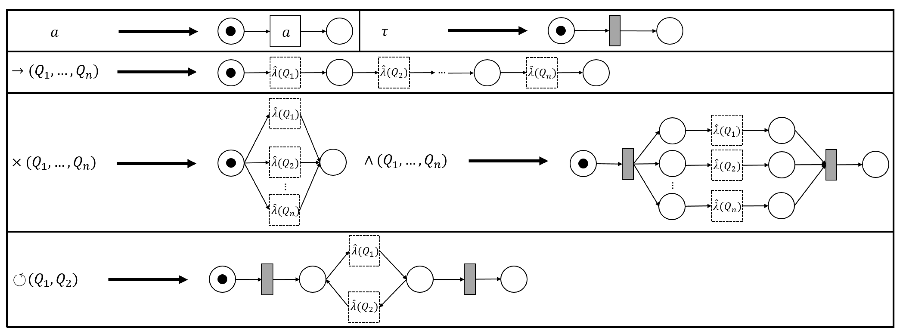
The process tree operators that we consider in this paper (→, ×, ∧ and ⥀) are easily translated to sound WF-nets (cf. Figure 5). Hence, we define a generic process tree to WF-net translation function, s.t., the language of the two is the same.

Definition 5 (Process Tree Transformation Function).

Let$Q\in \mathcal{Q}$be a process tree. A process tree transformation function λ, is a function$\lambda :\mathcal{Q}\to \mathcal{W}$, s.t., ${\mathcal{L}}_{\mathcal{N}}^{\nu }(\lambda (Q))={\mathcal{L}}_{\mathcal{Q}}(Q)$. We let$\widehat{\lambda }:\mathcal{Q}\to \mathcal{N}$, where, given$\lambda (Q)=W=(P,T,F,p_i,p_o,\ell )$, $\widehat{\lambda }(Q)=(P^{\prime },T,F^{\prime },\ell )$, with, $P^{\prime }=p\backslash \{p_i,p_o\}$and$F^{\prime }=F\backslash \left(\{(p_i,t)\in F\}\cup \{(t,p_o)\in F\}\right)$.

Given an arbitrary process tree $Q\in \mathcal{Q}$, there are several ways to translate it to a sound WF-net W, s.t., ${\mathcal{L}}_{\mathcal{N}}^{\nu }(W)={\mathcal{L}}_{\mathcal{Q}}(Q)$, i.e., instantiating $\lambda$ and $\widehat{\lambda }$. As an example, consider the translation functions, depicted in Figure 5.

Note that each transformation function in Figure 5 is sound by construction. Interestingly, recursively inserting the $\widehat{\lambda }$-generated fragments of the sub-trees of a given process tree, corresponds to the sequential application of WF-net composition, as described in [17], [Section 7]. Hence, we deduce that their recursive composition also results in a sound WF-net [17], [Theorem 3.3]. Note that, in the remainder of this paper, we explicitly assume the use of $\lambda$, as presented in Figure 5, i.e., certain proofs presented later build upon the recursive nature of the translations ad presented in Figure 5.

3. Translating Workflow Nets to Process Trees

In this section, we describe our approach. In Section 3.1, we sketch the main idea of the approach, using a small example. In Section 3.2, we present PTree-nets, i.e., Petri nets with $rng(\ell )=\mathcal{Q}$, which we exploit in our approach. In Section 3.3, we present Petri net fragments, used to identify process tree operators within the net, together with a generic reduction function. Finally, in Section 3.4, we provide an algorithmic description that allows us to find process trees, including correctness proofs.

3.1. Overview

The core idea of the approach concerns searching for fragments in the given WF-net that represent behavior that is expressible as a process tree. The patterns we look for bear significant similarity with the translation patterns defined in Figure 5, i.e., they can be considered as a strongly generalized reverse of those patterns. When we find a pattern, we replace it with a smaller net fragment representing the process tree that was identified. We continue to search for patterns in the reduced net until we are not able to find any more patterns. As we prove in Section 3.4, in the case the final WF-net contains just one transition, its label carries a process tree with the same labeled-language as the original WF-net.

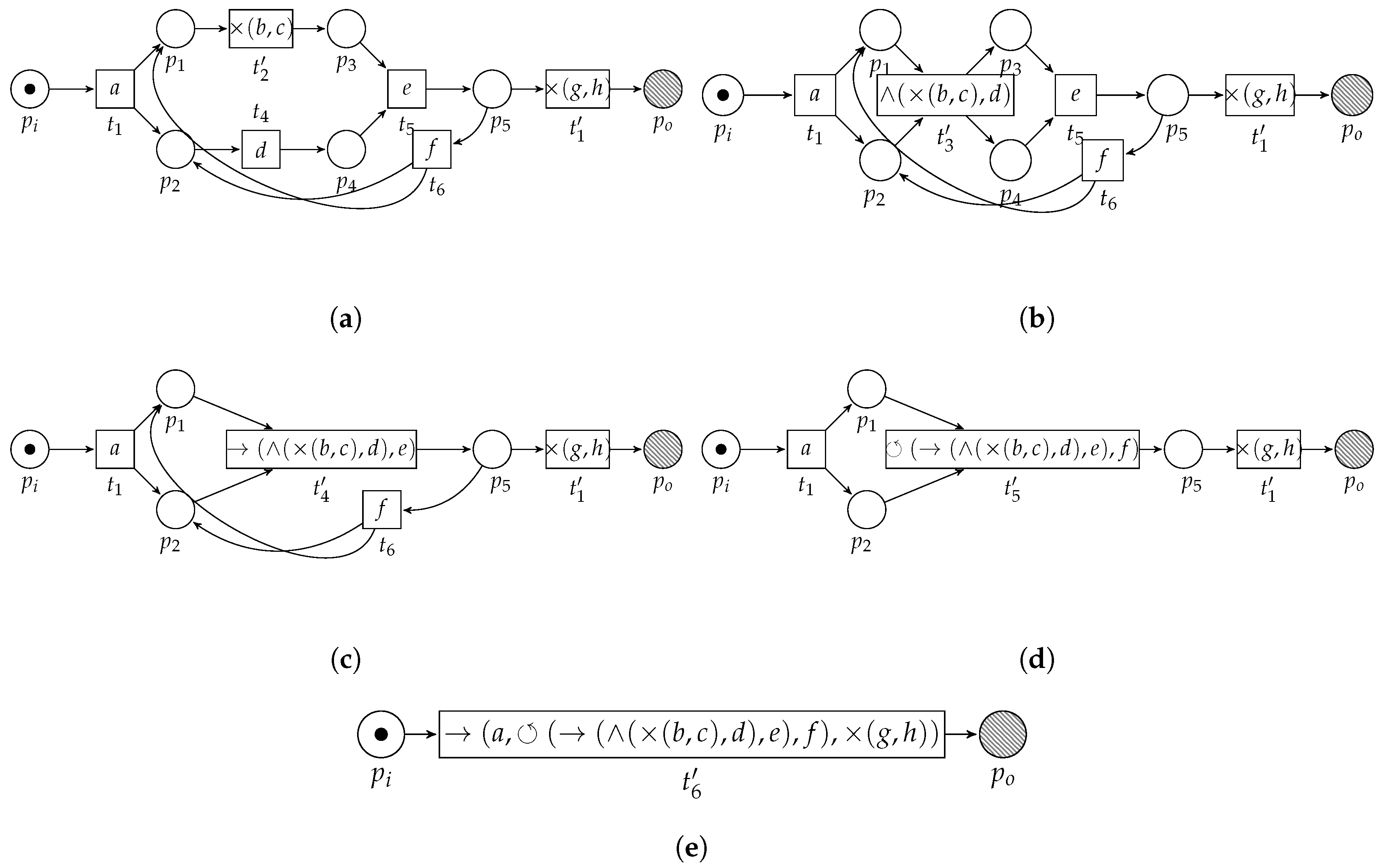
Consider Figure 6, in which we sketch the basic idea of the algorithm, applied on the example WF-net $W_1$ (Figure 3). First, the algorithm detects two choice constructs, i.e., one between the transitions labeled b and c and one between the transitions labeled g and h. The algorithm replaces the fragments by means of two new transitions, carrying labels $\times (b,c)$ and $\times (g,h)$, respectively (Figure 6a). Subsequently, a concurrent construct is detected, i.e., between the transitions labeled $\times (b,c)$ and d. Again, the pattern is replaced (Figure 6b). A sequential pattern is detected and replaced (Figure 6c), after which a loop construct is detected (Figure 6d). The resulting process tree, i.e., carried by the remaining transition in Figure 6e, $\to (a,⥀(\to (\wedge (\times (b,c),d),e),f),\times (g,h))$, is equal to Figure 4.

3.2. PTree-Nets and Their Unfolding

As indicated, we aim to find Petri net fragments in the WF-net representing behavior equivalent to a process tree. As illustrated in Section 3.1, the patterns found in the WF-net are replaced by transitions with a label carrying a corresponding process tree. In the upcoming section, we present four different fragment characterizations, corresponding to the basic process tree operators considered. However, in this section, we first briefly present PTree-nets, i.e., a trivial extension of Petri nets, in which labels are process trees.

Definition 6 (Process Tree-labeled Petri-net (PTree-net)).

Let$\mathcal{Q}$denote the universe of process trees. Let P denote a set of places, let T denote a set of transitions, let$F\subseteq (P\times T)\cup (T\times P)$denote the arc relation and let$\kappa :T\to \mathcal{Q}$. Tuple$N=(P,T,F,\kappa )$is a Process Tree-labeled Petri net (PTree-net). ${\mathcal{N}}_{\mathcal{Q}}$denotes the universe of PTree-nets.

Given $N\in {\mathcal{N}}_{\mathcal{Q}}$, for any marking $M,M^{\prime }$, we have $\kappa \left({\mathcal{L}}_{\mathcal{N}}\left(N,M,M^{\prime }\right)\right)\in {\mathcal{Q}}^{*}$ and ${\mathcal{L}}_{\mathcal{Q}}\left(\kappa \left({\mathcal{L}}_{\mathcal{N}}\left(N,M,M^{\prime }\right)\right)\right)\in {\Sigma }^{*}$, i.e., the definition of ${\mathcal{L}}_{\mathcal{Q}}$ ignores $\tau \notin \Sigma$ (observe: ${\mathcal{L}}_{\mathcal{N}}^{\nu }\left(N,M,M^{\prime }\right)=\kappa {\left({\mathcal{L}}_{\mathcal{N}}\left(N,M,M^{\prime }\right)\right)}_{{\downarrow }_{\Sigma }}={\mathcal{L}}_{\mathcal{Q}}\left(\kappa \left({\mathcal{L}}_{\mathcal{N}}\left(N,M,M^{\prime }\right)\right)\right)$). Clearly, since PTree-nets extend the labelling function to $\mathcal{Q}$, PTree-System-nets, and PTree-WF-nets are readily defined. We let ${\mathcal{SN}}_{\mathcal{Q}}$ and ${\mathcal{W}}_{\mathcal{Q}}$ represent their respective universes. Note that we use a different symbol to indicate whether a labeling function maps to $\mathcal{Q}$ or $\Sigma \cup \{\tau \}$, i.e., $\kappa :T\to \mathcal{Q}$, whereas $\ell :T\to \Sigma \cup \{\tau \}$.

Since a PTree-net contains process trees as its labels, which can be translated into a Petri net fragment, we define a PTree-net unfolding, cf. Definition 7, which maps a PTree-net onto a corresponding conventional Petri net.

Definition 7 (PTree-net Unfolding).

A PTree-net unfolding$\mathrm{\Lambda }:{\mathcal{N}}_{\mathcal{Q}}\to \mathcal{N}$is a function where, given$N=(P,T,F,\kappa )\in {\mathcal{N}}_{\mathcal{Q}}$, $\mathrm{\Lambda }(N)=(P^{\prime },T^{\prime },F^{\prime },\ell )$, with:

Let$\lambda (\kappa (t))=(P_t,T_t,F_t,p_{i_t},p_{o_t},{\ell }_t)$and$\widehat{\lambda }(\kappa (t))=({\widehat{P}}_t,{\widehat{T}}_t,{\widehat{F}}_t,{\widehat{\ell }}_t),\forall t\in T$,

1. 

$P^{\prime }=P\cup {\displaystyle \bigcup _{t\in T}}{\widehat{P}}_t$,

2. 

$T^{\prime }={\displaystyle \bigcup _{t\in T}}{\widehat{T}}_t$,

3. 

$F^{\prime }={\displaystyle \bigcup _{t\in T}}{\widehat{F}}_t\cup {\displaystyle \bigcup _{t\in T}}\{(p,t)\mid p\in •t\wedge t\in p_{i_t}•\}\cup {\displaystyle \bigcup _{t\in T}}\{(t,p)\mid p\in t•\wedge t\in •p_{o_t}\}$,

4. 

$\ell ={\displaystyle \bigcup _{t\in T}}{\widehat{\ell }}_t$. (Since functions are binary Cartesian products, we write set operations here).

Observe that, under the assumption that we use the instantiation of $\lambda$ as shown in Figure 5, indeed, each transition in the unfolding of a PTree-net has a corresponding label in $\Sigma \cup \{\tau \}$. Furthermore, note that unfolding the WF-net in Figure 6a yields the original model in Figure 3. The unfolding of the other WF-nets in Figure 6 yields a different WF-net. However, the language of all unfolded WF-nets remains equal to the language of the WF-net in Figure 3.

3.3. Pattern Reduction

In this section, we describe four patterns used to identify and replace process tree behavior. Furthermore, we propose a corresponding overarching reduction function, which shows how to reduce a PTree-WF-net containing any of these patterns. However, first, we present the general notion of a feasible pattern. Such a feasible pattern is a system net, formed by a place-bordered fragment of a given PTree-net. Furthermore, the language of the unfolding of the system net needs to be equal to the language of the process tree it represents. We formalize the notion of a feasible pattern as follows.

Definition 8 (Feasible Pattern).

Let ⨁ denote the universe of process tree operators. Let $N=(P,T,F,\kappa )\in {\mathcal{N}}_{\mathcal{Q}}$, let $N^{\prime }=(P^{\prime },T^{\prime }=\left\{t_1,\dots ,t_n\right\},F^{\prime },\kappa {|}_{T^{\prime }})⊑N$ be a place-bordered fragment of N ($N^{\prime }⊑N$) with corresponding input places $P_i^{\prime }$ and output places $P_o^{\prime }$. Let $M_i=P_i$ and $M_f=P_o$. Given $\oplus \in ⨁$, $SN=(N^{\prime },M_i,M_f)\in {\mathcal{SN}}_{\mathcal{Q}}$ is a feasible ⊕-pattern, written ${\theta }_{\oplus }(N,SN)$, iff:

$${\mathcal{L}}_{\mathcal{Q}}\left(\oplus \left(\kappa \left(t_1\right),...,\kappa \left(t_n\right)\right)\right)={\mathcal{L}}_{\mathcal{N}}^{\nu }\left(\mathrm{\Lambda }\left(N^{\prime }\right),M_i,M_f\right)$$

(1)

Observe that any place-bordered fragment of a WF-net that describes the same local language as its corresponding process tree representation is a feasible pattern. As such, any feasible pattern is locally language-preserving. Transforming such a detected pattern within the given WF-net is straightforward, i.e., we add a new transition $t^{\prime }$ to the WF-net with label $\oplus \left(\kappa \left(t_1\right),\dots ,\kappa \left(t_n\right)\right)$ and pre-set $P_i$ and post-set $P_o$. For example, consider the reduction of the choice construct between transitions $t_2$ and $t_3$ of Figure 3, i.e., depicted in Figure 6a, in which places $p_1$ and $p_3$ serve as the pre- and post-set of the newly added transition $t_2^{\prime }$ with label $\times (b,c)$. We formally define the notion of feasible pattern reduction as follows.

Definition 9 (Pattern Reduction).

Let$\oplus \in \{\to ,\times ,\wedge ,⥀\}$, let$N=(P,T,F,\kappa )\in {\mathcal{N}}_{\mathcal{Q}}$, let$N^{\prime }=(P^{\prime },T^{\prime }=\left\{t_1,\dots ,t_n\right\},F^{\prime },\kappa {|}_{T^{\prime }})⊑N$be a place-bordered fragment of N with corresponding input places$P_i$and output places$P_o$. Let$M_i=P_i$, $M_f=P_o$and let$SN=\left(N^{\prime },M_i,M_f\right)$s.t.${\theta }_{\oplus }(N,SN)$. We let${\Theta }_{\oplus }(N,SN)=N^{\prime \prime }=(P^{\prime \prime },T^{\prime \prime },F^{\prime \prime },{\kappa }^{\prime })$denote the${\theta }_{\oplus }(N,SN)$-reduced PTree-net, with, for$t^{\prime }\notin T$:

$$\begin{array}{c}\hfill P^{\prime \prime }=(P\backslash P^{\prime })\cup P_i\cup P_o\\ \hfill T^{\prime \prime }=\left(T\backslash T^{\prime }\right)\cup \{t^{\prime }\}\\ \hfill F^{\prime \prime }=(F\backslash F^{\prime })\cup \{(p,t^{\prime })\mid p\in P_i\}\cup \{(t^{\prime },p)\mid p\in P_o\}\\ \hfill {\kappa }^{\prime }{=\kappa |}_{T\backslash T^{\prime }}\cup \{(t^{\prime },\oplus (\kappa (t_1),...,\kappa (t_n)))\}\end{array}$$

A feasible pattern${\theta }_{\oplus }(N,SN)$is globally language preserving iff$\forall M,M^{\prime }\in \mathcal{M}(P^{\prime \prime })\left({\mathcal{L}}_{\mathcal{N}}^{\nu }(\mathrm{\Lambda }(N),M,M^{\prime })={\mathcal{L}}_{\mathcal{N}}^{\nu }(\mathrm{\Lambda }(N^{\prime \prime }),M,M^{\prime })\right)$

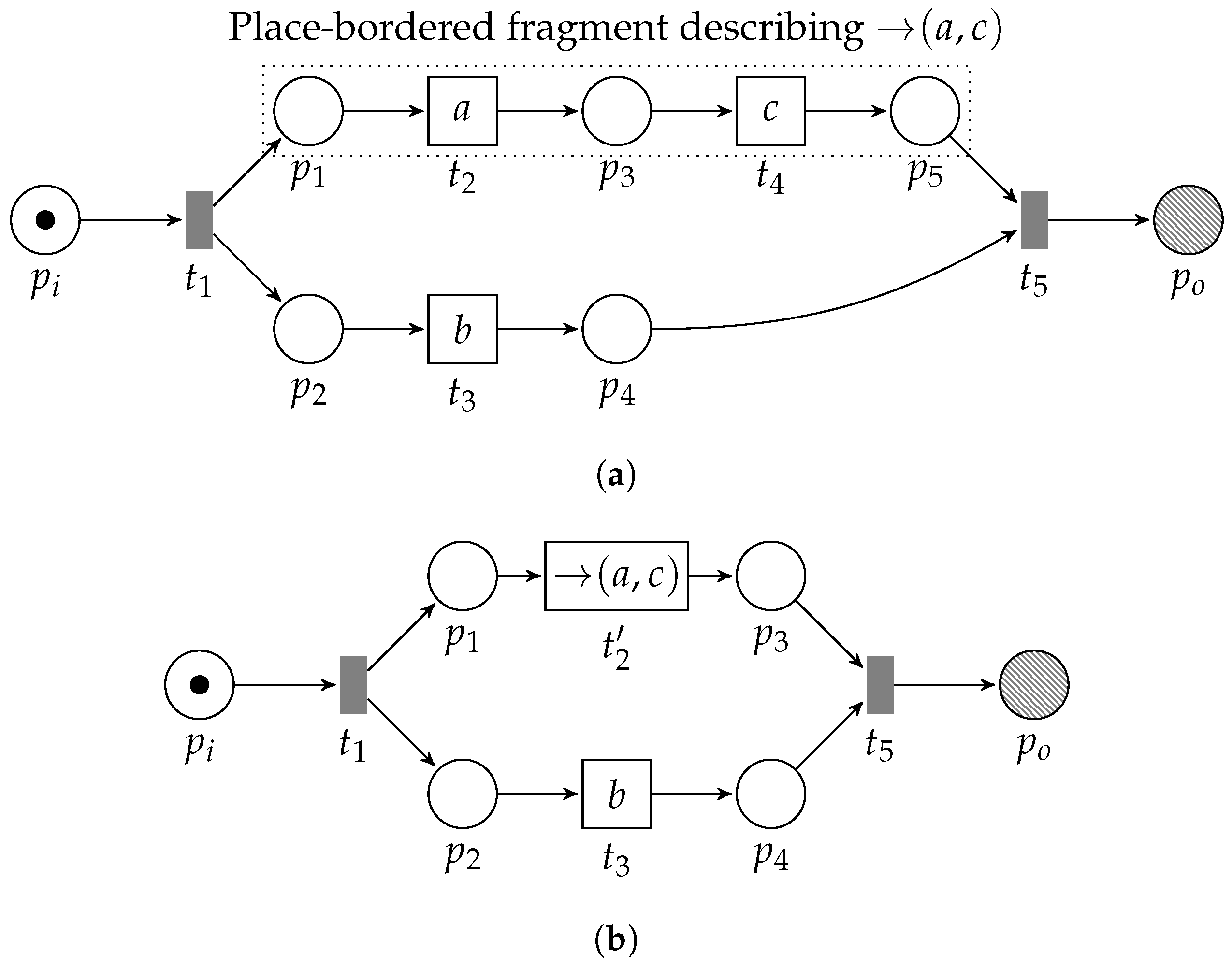
It is important to note that the notion of globally language-preserving is defined on the unfolding of a net and its corresponding reduced net. For example, consider Figure 7. In the WF-net in Figure 7a, we observe concurrent behavior between a sequential construct between a and c, and, activity b. The fragment formed by $p_1$, $p_3$, $p_5$, $t_2$, and $t_4$, is a feasible sequence pattern. In Figure 7b, we depict the reduced counterpart of the net in Figure 7a, in which transitions $t_2$ and $t_4$, and the place connecting them, i.e., $p_3$, are replaced by transition $t_2^{\prime }$ with label $\to (a,c)$. Observe that the language of the original net (Figure 7a) is $\{\langle t_1,t_2,t_3,t_4,t_5\rangle ,\langle t_1,t_3,t_2,t_4,t_5\rangle ,\langle t_1,t_2,t_4,t_3,t_5\rangle \}$, whereas the language of the corresponding reduced net (Figure 7b) is $\{\langle t_1,t_2^{\prime },t_3,t_5\rangle ,\langle t_1,t_3,t_2^{\prime },t_5\rangle \}$. Consequently, the corresponding labeled languages are $\{\langle a,b,c\rangle ,\langle b,a,c\rangle ,\langle a,c,b\rangle \}$ and $\{\langle \to (a,c),b\rangle ,\langle b,\to (a,c)\rangle \}$, respectively. The labeled language of the reduced net, after evaluating the process tree fragments inside, yields $\{\langle a,c,b\rangle ,\langle b,a,c\rangle \}$, i.e., the trace $\langle a,b,c\rangle$ is not in the corresponding language. However, if we first unfold the label of $t_2^{\prime }$ in Figure 7b, i.e., yielding the model in Figure 7a (modulo renaming of transitions), the labeled languages of the two nets are indeed equal, i.e., they both describe $\{\langle a,b,c\rangle ,\langle b,a,c\rangle ,\langle a,c,b\rangle \}$.

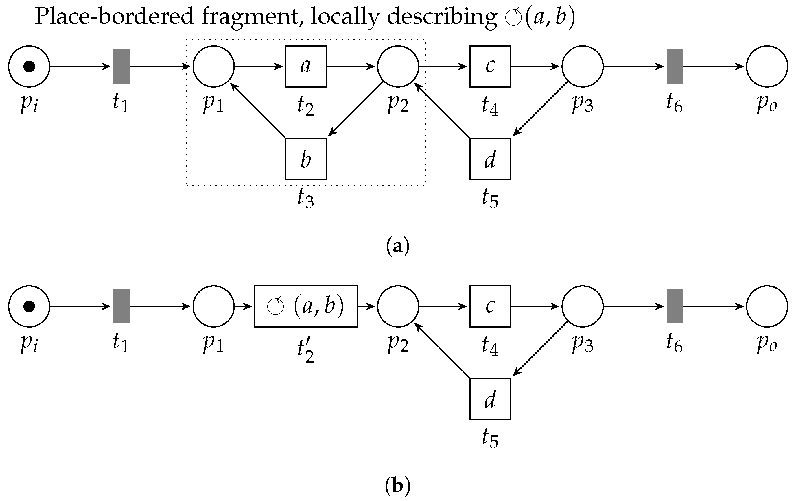
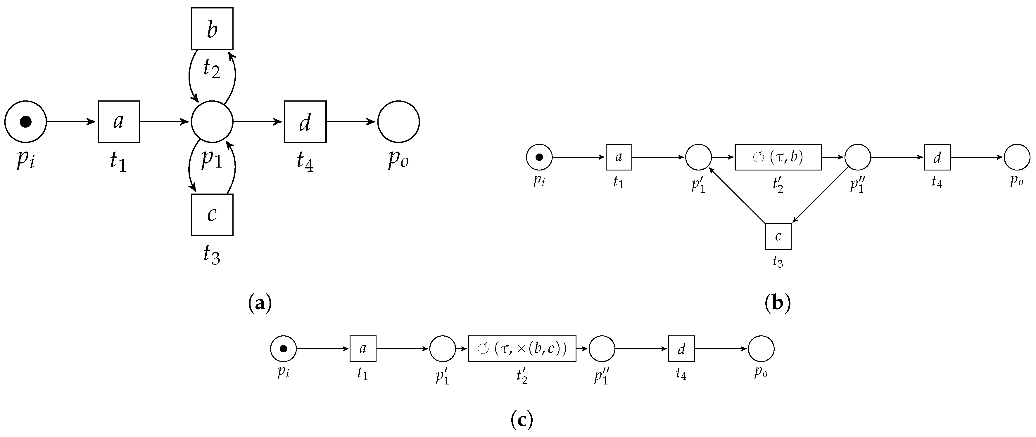
Furthermore, observe that there exist feasible patterns that are locally language-preserving, yet, not globally language-preserving. For example, consider the WF-net in Figure 8. The place-bordered fragment formed by the subnet consisting of places $p_1$ and $p_2$ and transitions $t_2$ and $t_3$ (with the arcs connecting them), form a feasible pattern corresponding to $⥀(a,b)$ (with $M_i=[p_1]$ and $M_f=[p_2]$). However, note that, after reduction, i.e., by inserting $t_2^{\prime }$, we obtain a WF-net that no longer has the same language as the original model. This is because, before reduction, executing transition $t_5$ allows us to enable transition $t_3$. After reduction, however, this is no longer possible. Hence, whereas the observed feasible pattern is locally language preserving, i.e., when considering the elements it is composed of, it is not globally language-preserving.

In the upcoming paragraphs, we characterize an instantiation of a global language preserving feasible pattern for each process tree operator considered in this paper. For each proposed pattern, we prove that it is both locally and globally language preserving.

3.3.1. Sequential Pattern

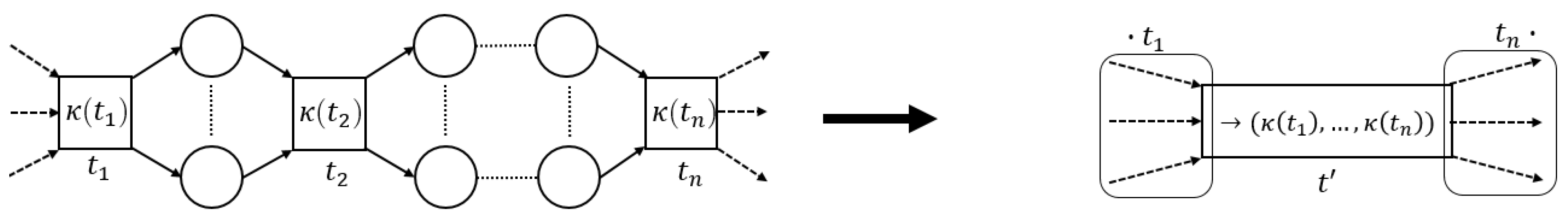
The →-operator, i.e., $\to \left(Q_1,...,Q_n\right)$, describes sequential behavior, hence, any subnet describing strictly sequential behavior, describes the same language. If a transition $t_1$ always, uniquely, enables transition $t_2$, which in turn enables transition $t_3,\dots ,t_n$, and, whenever $t_1$ has fired, the only way to consume all tokens from $t_1•$ is by means of firing $t_2$, and, similarly, the only way to consume all tokens from $t_2•$ is by means of firing $t_3$, etc.; then, $t_1,\dots ,t_n$ are in a sequential relation. We visualize the →-pattern in the left-hand side of Figure 9. Note that, in the visualization, we omit $P_i$ and $P_o$, respectively, i.e., $•t_1$ and $t_n•$.

We formally define the notion of a sequential pattern as follows

Proposition 1 (→-Pattern).

Let$N=(P,T,F,\kappa )\in {\mathcal{N}}_{\mathcal{Q}}$and let$T^{\prime }=\left\{t_1,\dots ,t_n\right\}\subseteq T$ ($n\ge 2$). If and only if:

1. 

$\forall 1\le i<n\left(|t_i•|\ge 1\wedge t_i•=•t_{i+1}\right)$, transition$t_i$enables$t_{i+1}$; and

2. 

$\forall 1\le i<n\left(\forall p\in t_i•\left(•p=\{t_i\}\wedge p•=\{t_{i+1}\}\right)\right)$, enabling is unique,

then, system net $SN=(N^{\prime }=(P^{\prime },T^{\prime },F^{\prime },\kappa {|}_{T^{\prime }}),•t_1,t_n•)$ ($P_i=•t_1$ and $P_o=t_n•$), with $P^{\prime }=•t_1\cup •t_2\cup \dots •t_n\cup t_n•$, $F^{\prime }=\{(x,y)\in F\mid y\in T^{\prime }\vee x=t_n\}$, is a feasible →-pattern.

Proof. 

Observe that $t_1$ is the only enabled transition in marking $M_i=P_i$. By definition of the proposed pattern, after firing $t_i$ ($1\le i<n$), the only enabled transition is $t_{i+1}$. After firing $t_n$, we reach the final marking $M_f$, which is a deadlock marking (the only deadlock marking) of the place-bordered subnet. Hence, any firing sequence of $\mathrm{\Lambda }(N^{\prime })$ can be written as ${\sigma }_1·{\sigma }_2\cdots {\sigma }_n$, s.t., $(\mathrm{\Lambda }(N^{\prime }),M_i)\stackrel{{\sigma }_1}{\twoheadrightarrow }(\mathrm{\Lambda }(N^{\prime }),t_1•)\stackrel{{\sigma }_2}{\twoheadrightarrow }\cdots \stackrel{{\sigma }_n}{\twoheadrightarrow }(\mathrm{\Lambda }(N^{\prime }),M_f)$. Observe that each element of ${\sigma }_1$ is a transition in $\lambda (\kappa (t_1))$, each element of ${\sigma }_2$ is a transition in $\lambda (\kappa (t_2))$, etc. Furthermore, by definition of λ, ${\sigma }_1$ is a firing sequence describing (when projected on its visible labels) a memmber of ${\mathcal{L}}_{\mathcal{Q}}(\kappa (t_1))$, ${\sigma }_2$ describes as sequence in ${\mathcal{L}}_{\mathcal{Q}}(\kappa (t_1))$, etc. Hence, the set of all firing sequences projected on their visible labels equals ${\mathcal{L}}_{\mathcal{Q}}(\to (\kappa (t_1),\kappa (t_2),\dots ,\kappa (t_n)))$. □

Lemma 1 (→-Pattern (Proposition 1) is Globally Language-Preserving).

Let$N=(P,T,F,\kappa )\in {\mathcal{N}}_{\mathcal{Q}}$and let$SN=(N^{\prime }=(P^{\prime },T^{\prime }=\{t_1,t_2,\dots ,t_n\},F^{\prime },\kappa {|}_{T^{\prime }}),•t_1,t_n•)$s.t.${\theta }_{\to }(N,SN)$according to$Proposition$ 1. The feasible pattern ${\theta }_{\to }(N,SN)$ is globally language-preserving.

Proof. 

Let $N^{\prime \prime }$ denote the net obtained after reduction (cf. Definition 9) and let $P^{\prime \prime }=(P\backslash P^{\prime })\cup P_i\cup P_o$. We need to prove that $\forall M,M^{\prime }\in \mathcal{M}(P^{\prime \prime })\left({\mathcal{L}}_{\mathcal{N}}^{\nu }(\mathrm{\Lambda }(N),M,M^{\prime })={\mathcal{L}}_{\mathcal{N}}^{\nu }(\mathrm{\Lambda }(N^{\prime \prime }),M,M^{\prime })\right)$.

Observe that $\mathrm{\Lambda }(N)$ and $\mathrm{\Lambda }(N^{\prime \prime })$ are identical, except for $\mathrm{\Lambda }(N^{\prime })$ in N and $\widehat{\lambda }(t^{\prime })$ (the transition-bordered unfolding of the newly added transition $t^{\prime }$) in $N^{\prime \prime }$, respectively. The only connections between $N^{\prime }$ in N and $t^{\prime }$ in $N^{\prime \prime }$ with the identical parts of the two nets are through $P_i$ and $P_o$. Hence, if there exists a visible firing sequence in ${\mathcal{L}}_{\mathcal{N}}^{\nu }(\mathrm{\Lambda }(N),M,M^{\prime })$ that is not in ${\mathcal{L}}_{\mathcal{N}}^{\nu }(\mathrm{\Lambda }(N^{\prime \prime }),M,M^{\prime })$, this can only be due to different behavior described by $\mathrm{\Lambda }(N^{\prime })$ and $\lambda (t^{\prime })$. However, this directly contradicts feasibility of the pattern. □

3.3.2. Exclusive Choice Pattern

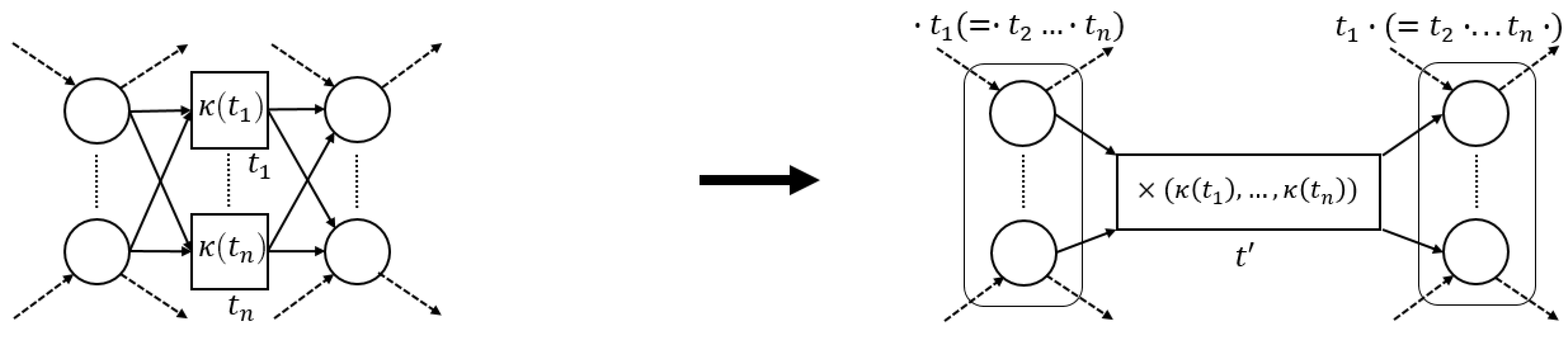
The ×-operator, i.e., $\times (Q_1,\dots ,Q_n)$, describes “execute one of $Q_1,\dots ,Q_n$”. In terms of a Petri net fragment, transitions $t_1,\dots ,t_n$ are in an exclusive choice pattern if their pre- and post-sets are equal (yet non-overlapping). Consider Figure 10, in which we schematically depict the ×-pattern.

We formalize the ×-pattern as follows.

Proposition 2 (×-Pattern).

Let$N=(P,T,F,\kappa )\in {\mathcal{N}}_{\mathcal{Q}}$and let$T^{\prime }=\left\{t_1,\dots ,t_n\right\}\subseteq T$ ($n\ge 2$). If and only if:

1. 

$•t_1=•t_2=\cdots =•t_n$, all pre-sets are shared among the members of the pattern;

2. 

$t_1•=t_2•=\cdots =t_n•$, all post-sets are shared among the members of the pattern; and

3. 

$\forall 1\le i\le n\left(•t_i\ne t_i•\right)$, self-loops are not allowed,

then, system net $SN=\left(N^{\prime }=\left(P^{\prime },T^{\prime },F^{\prime }{,\kappa |}_{T^{\prime }}\right),•t_1,t_1•\right)$ ($P_i=•t_1$ and $P_o=t_1•$), with $P^{\prime }=•t_1\cup t_1•$, $F^{\prime }=\{(x,y)\in F\mid x\in T^{\prime }\vee y\in T^{\prime }\}$, is a feasible ×-pattern.

Proof. 

Observe that $t_1,t_2,\dots ,t_n$ are the only enabled transitions in $N^{\prime }$ in marking $M_i=P_i$. When we fire any one of these transitions, we immediately mark $P_o$, which is the final marking of the system net. Hence, the set of firing sequences of the system net is the union of the set of sequences $(\mathrm{\Lambda }(N^{\prime }),M_i)\stackrel{\sigma }{\twoheadrightarrow }(\mathrm{\Lambda }(N^{\prime }),M_i)$, where σ either corresponds to a labelled language of ${\mathcal{L}}_{\mathcal{Q}}(\kappa (t_1)$, or ${\mathcal{L}}_{\mathcal{Q}}(\kappa (t_2)$, …, or ${\mathcal{L}}_{\mathcal{Q}}(\kappa (t_n)$. Observe that, indeed, this set corresponds to ${\mathcal{L}}_{\mathcal{Q}}(\times (\kappa (t_1),\kappa (t_2),\dots ,\kappa (t_n)))$. □

Lemma 2 (×-Pattern (Proposition 2) is Globally Language-Preserving).

Let$N=(P,T,F,\kappa )\in {\mathcal{N}}_{\mathcal{Q}}$and let$SN=(N^{\prime }=(P^{\prime },T^{\prime }=\{t_1,t_2,\dots ,t_n\},F^{\prime },\kappa {|}_{T^{\prime }}),•t_1,t_1•)$s.t.${\theta }_{\times }(N,SN)$according to$Proposition$ 2. The feasible pattern ${\theta }_{\times }(N,SN)$ is globally language-preserving.

Proof. 

Let $N^{\prime \prime }$ denote the net obtained after reduction (cf. Definition 9) and let $P^{\prime \prime }=(P\backslash P^{\prime })\cup P_i\cup P_o$. Observe that, similar to the sequential pattern, $\mathrm{\Lambda }(N)$ and $\mathrm{\Lambda }(N^{\prime \prime })$ are identical, except for $\mathrm{\Lambda }(N^{\prime })$ and $\widehat{\lambda }(t^{\prime })$, respectively. Again, the only connections between $N^{\prime }$ and $t^{\prime }$ with the identical parts of the two nets are through $P_i$ (“entering”) and $P_o$(“exiting”). Hence, if there exists a visible firing sequence in ${\mathcal{L}}_{\mathcal{N}}^{\nu }(\mathrm{\Lambda }(N),M,M^{\prime })$ that is not in ${\mathcal{L}}_{\mathcal{N}}^{\nu }(\mathrm{\Lambda }(N^{\prime \prime }),M,M^{\prime })$, this can only be due to different behavior described by $\mathrm{\Lambda }(N^{\prime })$ and $\lambda (t^{\prime })$, again contradicting the feasibility of the pattern. □

3.3.3. Concurrent Pattern

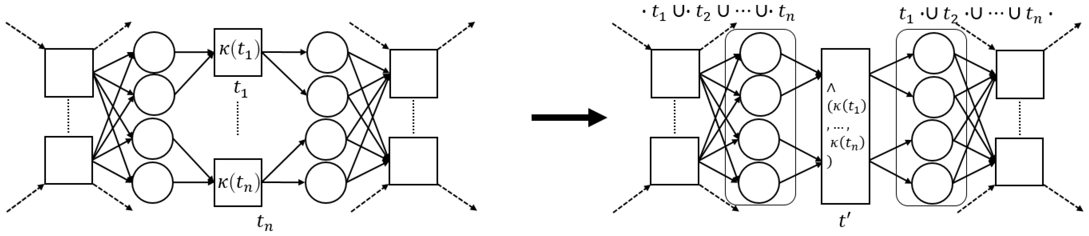
The concurrent pattern is the most complicated pattern that we consider in this paper. In the concurrent pattern, interference between its transitions is possible. The interference is achieved by requiring that the pre-sets and post-sets of the transitions do not have any overlap. Furthermore, the pre-set of the transition’s pre-set places needs to be shared by all of these places, and, symmetrically, the post-set of the transition’s post-set places needs to be shared by all of these places. That is, the enabling of the transitions in the pattern needs to be the same, and their post-set should jointly block any further action (i.e., within its local scope) until all places in their joint post-set are marked. Consider the left-hand side of Figure 11, in which we schematically depict the concurrent pattern, which we formalize in Proposition 3.

Proposition 3 (∧-Pattern).

Let$N=(P,T,F,\kappa )\in {\mathcal{N}}_{\mathcal{Q}}$and let$T^{\prime }=\left\{t_1,\dots ,t_n\right\}\subseteq T$ ($n\ge 2$). If and only if:

1. 

$\forall 1\le i<j\le n\left(•t_i\cap •t_j=\varnothing \right)$, no interaction between the member’s pre-sets;

2. 

$\forall 1\le i<j\le n\left(t_i•\cap t_j•=\varnothing \right)$, no interaction between the member’s post-sets;

3. 

$\forall 1\le i\le n\left(\forall p\in •t_i\left(p•=\left\{t_i\right\}\right)\right)$, pre-set places uniquely connect to a member;

4. 

$\forall 1\le i\le n\left(\forall p\in t_i•\left(•p=\left\{t_i\right\}\right)\right)$, post-set places uniquely connect to a member;

5. 

$\forall p\in •T\left(•p\cap \{t_1,...,t_n\}=\varnothing \right)$, members do not influence other members;

6. 

$\forall p,p^{\prime }\in •T\left(•p=•p^{\prime }\right)$, member’s pre-sets share their pre-set;

7. 

$\forall p\in T•\left(p•\cap \{t_1,...,t_n\}=\varnothing \right)$, member firing does not affect other members;

8. 

$\forall p,p^{\prime }\in T•\left(p•=p^{\prime }•\right)$, member’s post-sets share their post-set;

9. 

$\forall t,t^{\prime }\in •\left(•T\right)\left(•t=•t^{\prime }\right)$, pre-sets of enablers are equal;

10. 

$\forall t,t^{\prime }\in \left(T•\right)•\left(t•=t^{\prime }•\right)$, post-sets of enablers are equal,

then, system net $SN=\left(N^{\prime }=\left(P^{\prime },T^{\prime },F^{\prime }{,\kappa |}_{T^{\prime }}\right),•T^{\prime },T^{\prime }•\right)$ ($P_i=•T^{\prime }$, $P_o=T^{\prime }•$), with $P^{\prime }=•T\cup T•$, $F^{\prime }=\{(x,y)\in F\mid (x\in P^{\prime }\wedge y\in T^{\prime })\vee (x\in T^{\prime }\wedge y\in P^{\prime })\}$ is a feasible ∧-pattern.

Proof. 

Observe that $t_1,t_2,\dots ,t_n$ are the only enabled transitions in $N^{\prime }$ in marking $M_i=P_i$. Furthermore, since none of the transitions share any of their presets, the transitions can be fired in any order. Note that, by definition of the pattern, after all transitions have fired, we reach final marking $M_f$ (which is a deadlock in the place-bordered system net). Hence, the labeled language described by the pattern equals ${\mathcal{L}}_{\mathcal{Q}}(\kappa (t_1))\leftrightharpoons {\mathcal{L}}_{\mathcal{Q}}(\kappa (t_2))\cdots \leftrightharpoons {\mathcal{L}}_{\mathcal{Q}}(\kappa (t_n))$, which equals $\wedge \left(\kappa (t_1),\kappa (t_2),...,\kappa (t_n)\right)$. □

Lemma 3 (∧-Pattern (Proposition 3) is Globally Language-Preserving).

Let$N=(P,T,F,\kappa )\in {\mathcal{N}}_{\mathcal{Q}}$and let$SN=(N^{\prime }=(P^{\prime },T^{\prime }=\{t_1,t_2,\dots ,t_n\},F^{\prime },\kappa {|}_{T^{\prime }}),•t_1,t_1•)$s.t.${\theta }_{\wedge }(N,SN)$according to$Proposition$ 3. The feasible pattern ${\theta }_{\wedge }(N,SN)$ is globally language-preserving.

Proof. 

Observe that $\mathrm{\Lambda }(N)$ and $\mathrm{\Lambda }(N^{\prime \prime })$ are identical, except for $\mathrm{\Lambda }(N^{\prime })$ and $\widehat{\lambda }(t^{\prime })$, respectively. Again, the only connections between $N^{\prime }$ and $t^{\prime }$ with the identical parts of the two nets are through $P_i$ (“entering”) and $P_o$(“exiting”). Hence, if there exists a visible firing sequence in ${\mathcal{L}}_{\mathcal{N}}^{\nu }(\mathrm{\Lambda }(N),M,M^{\prime })$ that is not in ${\mathcal{L}}_{\mathcal{N}}^{\nu }(\mathrm{\Lambda }(N^{\prime \prime }),M,M^{\prime })$, this can only be due to different behavior described by $\mathrm{\Lambda }(N^{\prime })$ and $\lambda (t^{\prime })$, again contradicting the feasibility of the pattern. □

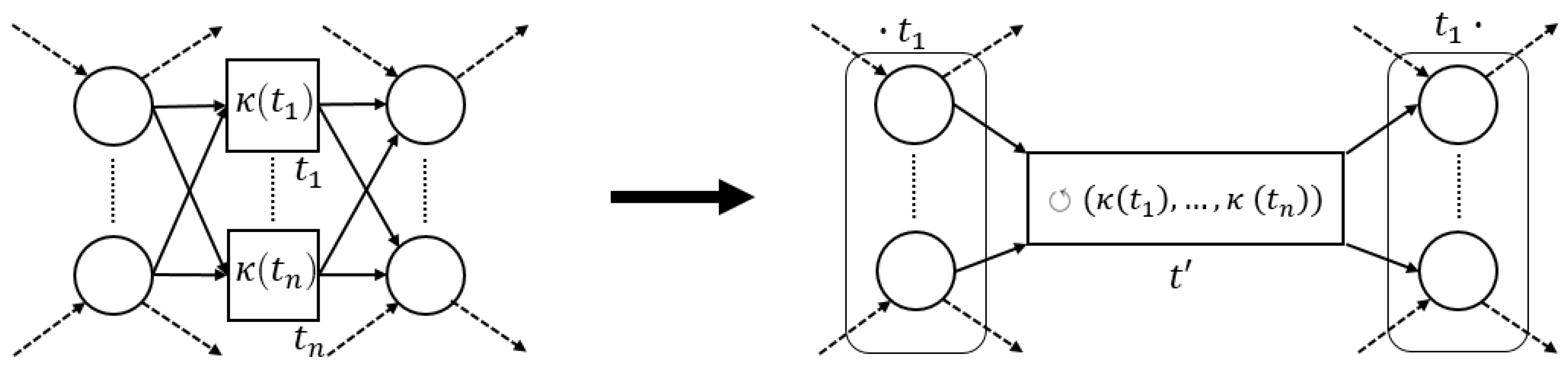
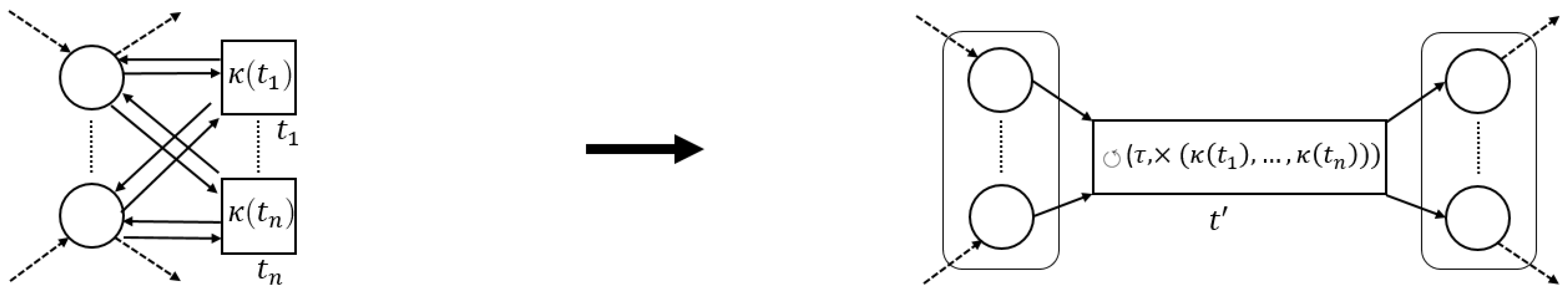
3.3.4. Loop Pattern

The final operator we consider is the ⥀-operator, i.e., the only operator with just two children. Hence, the fragments representing a loop pattern in the Ptree-net consist of two transitions. Consider the left-hand side of Figure 12, in which we schematically depict the loop pattern fragment. Conceptually, the loop operator requires us first to execute its leftmost child (the “do-part”). Secondly, its rightmost child is optionally executed (the “redo-part”). However, we always finish with the leftmost child. As such, the post-set of a transition corresponding to the do-part needs to be the pre-set of the transition that represents the redo-part. Furthermore, there should be no other way to enable the redo-part. Hence, the do-part needs to be the only transition that marks the pre-set of the redo-part. Similarly, to guarantee global language preservation, the do-part should be the only element in the post-set of its pre-set, i.e., no other transition may be enabled by the pre-set of the do-part. Reconsider Figure 8. Observe that $p_2$ contains multiple incoming and outgoing arcs; hence, it describes neither a loop-pattern for transitions $t_2$ and $t_3$ nor for transitions $t_4$ and $t_5$.

Proposition 4 (⥀-Pattern).

Let$N=(P,T,F,\kappa )\in {\mathcal{N}}_{\mathcal{Q}}$and let$t_1\ne t_2\in T$. Iff:

1. 

$•t_1=t_2•$, pre-set of$t_1$is the post-set of$t_2$;

2. 

$t_1•=•t_2$, pre-set of$t_2$is the post-set of$t_1$;

3. 

$\forall p\in •t_1\left(p•=\{t_1\}\right)$, $t_1$is the only transition in the post-set of its pre-set;

4. 

$\forall p\in t_1•\left(•p=\{t_1\}\right)$; $t_1$, is the only transition in the pre-set of its post-set,

then, system net$SN=\left(N^{\prime }=\left(P^{\prime },T^{\prime },F^{\prime }{,\kappa |}_{\{t_1,t_2\}}\right),•t_1,t_1•\right)$ ($P_i=•t_1$, $P_o=t_o•$), with $P^{\prime }=•t_1\cup t_1•$, $T^{\prime }=\{t_1,t_2\}$, $F^{\prime }=\{(x,y)\in F\mid x\in \{t_1,t_2\}\vee y\in \{t_1,t_2\}\}$ is a feasible ⥀-pattern.

Proof. 

Observe that $t_1$ is the only enabled transition in $N^{\prime }$ in marking $M_i=P_i$. When we fire it, we immediately mark $P_o$, which is the final marking of the place-bordered system net. In the aforesaid marking, $t_2$ is the only enabled transition. Firing $t_2$ yields us with marking $M_i$ again. We can repeat this infinitely. Hence, the labeled language described by the pattern is $\{{\sigma }_1·{\sigma }_1^{\prime }·{\sigma }_2·{\sigma }_2^{\prime }\cdots {\sigma }_n\mid n\ge 1\wedge \forall 1\le i\le n\left({\sigma }_i\in {\mathcal{L}}_{\mathcal{Q}}(\kappa (t_1))\right)\wedge \forall 1\le i<n\left({\sigma }_i^{\prime }\in {\mathcal{L}}_{\mathcal{Q}}(\kappa (t_2))\right)\}$, which equals $⥀\left({\mathcal{L}}_{\mathcal{Q}}(\kappa (t_1)),{\mathcal{L}}_{\mathcal{Q}}(\kappa (t_2))\right)$ □

Lemma 4 (⥀-Pattern (Proposition 4) is Globally Language-Preserving).

Let$N=(P,T,F,\kappa )\in {\mathcal{N}}_{\mathcal{Q}}$and let$SN=(N^{\prime }=(P^{\prime },T^{\prime }=\{t_1,t_2,\dots ,t_n\},F^{\prime },\kappa {|}_{T^{\prime }}),•t_1,t_1•)$s.t.${\theta }_{⥀}(N,SN)$according to$Proposition$ 4. The feasible pattern ${\theta }_{⥀}(N,SN)$ is globally language-preserving.

Proof. 

Let $N^{\prime \prime }$ denote the net obtained after reduction (cf. Definition 9) and let $P^{\prime \prime }=(P\backslash P^{\prime })\cup P_i\cup P_o$. Observe that $\mathrm{\Lambda }(N)$ and $\mathrm{\Lambda }(N^{\prime \prime })$ are identical, except for $\mathrm{\Lambda }(N^{\prime })$ and $\widehat{\lambda }(t^{\prime })$, respectively. Again, the only connections between $N^{\prime }$ and $t^{\prime }$ with the identical parts of the two nets are through $P_i$ (“entering”) and $P_o$(“exiting”). In particular, when $P_i$ is marked, the only way to mark $P_o$ is by firing $t_1$, followed by an arbitrary number of $\langle t_2,t_1\rangle$ repetitions. Hence, if there exists a visible firing sequence in ${\mathcal{L}}_{\mathcal{N}}^{\nu }(\mathrm{\Lambda }(N),M,M^{\prime })$ that is not in ${\mathcal{L}}_{\mathcal{N}}^{\nu }(\mathrm{\Lambda }(N^{\prime \prime }),M,M^{\prime })$, this can only be due to different behavior described by $\mathrm{\Lambda }(N^{\prime })$ and $\lambda (t^{\prime })$, contradicting the feasibility of the pattern. □

3.4. Algorithm

In this section, we present an algorithm that iteratively applies the reductions defined in Section 3.3. By doing so, the algorithm is able to translate a WF-net into a process tree. We prove that, if the algorithm terminates correctly, i.e., it finds a process tree, the input WF-net is sound. Moreover, we show that the language of the input WF-net equals the language of the process tree found.

Consider Algorithm 1, in which we present an algorithmic description of the reduction algorithm, on the basis of the proposed patterns in Section 3.3.

Algorithm 1: WF-net reduction

As an input, the algorithm needs any WF-net W, which, by definition, is also a PTWF-net. Initially, the elements of W, excluding the initial and final place, are copied into variables $P^{\prime },T^{\prime },F^{\prime },\kappa$. In case any pattern of the form ${\theta }_{\oplus }(N,SN)$ is found in N, the corresponding reduction ${\Theta }_{\oplus }(N,SN)$ is applied (line 1). If no more pattern is found, the algorithm returns $(N,p_i,p_o,\kappa )$. The algorithm returns the most recent reduction, if no more pattern is found. Observe that, intentionally, the order and size of the patterns to be reduced is not specified, i.e., it is of no relevance to any of the lemmas and the theorems regarding the algorithms properties and correctness.

In the case the obtained PTree-WF-net consists of just one transition, i.e., connected to place $p_i$ (incoming) and place $p_o$ (outgoing) (cf. Figure 6e), the label of the transition represents a process tree, describing the same language as the original WF-net. Furthermore, we can conclude that the original WF-net is, in fact, a sound WF-net. We prove these observations in Theorem 1. However, before this, we first present two useful lemmas. In Lemma 5, we prove that the proposed reduction rules are bidirectionally soundness preserving, i.e., if a PTree-WF-net is sound, the reduced PTree-WF-net is sound (and vice versa). In Lemma 6, we prove that, if we are able, from the initial marking $[p_i]$, to enable the observed fragment (enabling differs per fragment), then the language of the original net and the reduced net is equal (and vice versa). Observe that, trivially, the reduction rules applied on a PTree-WF-net yield a PTree-WF-net, i.e., none of the requirements of Definition 1 are violated on the resulting net.

Lemma 5 (Pattern Reduction is Soundness Preserving).

Let$\oplus \in \{\to ,\times ,\wedge ,⥀\}$, let$W=(P,T,F,p_i,p_o,\kappa )\in {\mathcal{W}}_{\mathcal{Q}}$, let$SN\in {\mathcal{SN}}_{\mathcal{Q}}$, s.t., ${\theta }_{\oplus }(W,SN)$, and let$W^{\prime }=(P^{\prime },T^{\prime },F^{\prime },p_i,p_o,{\kappa }^{\prime })={\Theta }_{\oplus }(W,SN)\in {\mathcal{W}}_{\mathcal{Q}}$. $W^{\prime }$is sound iff W is sound.

Proof. 

(⇒) Let $t^{\prime }\in T^{\prime }\backslash T$. Assume that W is sound, yet $W^{\prime }$ is not sound. By definition of any reduction ${\Theta }_{\oplus }(W,SN)$, if $W^{\prime }$ is not safe, then W is not safe. For any $t\in T\cap T^{\prime }$, if $\nexists M\in \mathcal{R}(W^{\prime },[p_i])\left((W^{\prime },M)[t\rangle \right)$, then also $\nexists M\in \mathcal{R}(W,[p_i])\left((W,M)[t\rangle \right)$. Similarly, if $\nexists M\in \mathcal{R}(W^{\prime },[p_i])\left((W^{\prime },M)[t^{\prime }\rangle \right)$, then this is also holds for the transitions in $SN$. In the case $\exists M\in \mathcal{R}(W^{\prime },[p_i])$ s.t. $\nexists \sigma \in T^{\prime *}\left((W^{\prime },M)\stackrel{\sigma }{\twoheadrightarrow }(W^{\prime },[p_o])\right)$, again, by definition of the reductions, also $M\in \mathcal{R}(W^{\prime },[p_i])$ and $\nexists \sigma \in T^{\prime *}\left((W,M)\stackrel{\sigma }{\twoheadrightarrow }(W,[p_o])\right)$, contradicting soundness of W.

(⇐) Assume that $W^{\prime }$ is sound, yet W is not sound. Given that $W^{\prime }$ and W only differ on $t^{\prime }$ and $SN$, respectively, the “non-sound” part of W needs to be part of $SN$. However, it is easy to see that none of the patterns defined in Section 3.3 do not describe any non-sound construct. Hence, replacing $SN$, implies that $W^{\prime }$ needs to be unsound, which contradicts the assumption. □

Lemma 6 (Pattern Reduction is Language Preserving in $\mathrm{\Lambda }$).

Let$\oplus \in \{\to ,\times ,\wedge ,⥀\}$, let$W=(P,T,F,p_i,p_o,\kappa )\in {\mathcal{W}}_{\mathcal{Q}}$, let$SN\in {\mathcal{SN}}_{\mathcal{Q}}$, s.t., ${\theta }_{\oplus }(W,SN)$, and, let$W^{\prime }=(P^{\prime },T^{\prime },F^{\prime },p_i,p_o,{\kappa }^{\prime })={\Theta }_{\oplus }(W,SN)\in {\mathcal{W}}_{\mathcal{Q}}$. ${\mathcal{L}}_{\mathcal{N}}^{\nu }(\mathrm{\Lambda }(W))={\mathcal{L}}_{\mathcal{N}}^{\nu }(\mathrm{\Lambda }(W^{\prime }))$.

Proof. 

It rrivially follows from Lemmas 1–4. □

Theorem 1 (Algorithm 1 is able to find Language-Equal Process Trees).

Let$W=\left(P,T,F,p_i,p_o,\ell \right)\in \mathcal{W}$and let$W^{\prime }=(P^{\prime },T^{\prime },F^{\prime },{p^{\prime }}_i,{p^{\prime }}_o,\kappa )\in {\mathcal{W}}_{\mathcal{Q}}$be the resulting WF-net of Algorithm 1 on W. If$P^{\prime }=\{P_i,P_o\}$, $T^{\prime }=\{t\}$, and$F=\left\{\left(p_i,t\right),\left(t,p_o\right)\right\}$, then${\mathcal{L}}_{\mathcal{Q}}(\kappa (t))={\mathcal{L}}_{\mathcal{N}}^{\nu }(W)$.

Proof. 

Observe that W is sound. Lemma 5 implies that if we (continuously) revert the reductions applied by Algorithm 1, i.e., corresponding to all intermediate assignments of W in Algorithm 1, all reverted nets are sound. As a corollary of this fact, it follows that W is sound. Observe that Lemma 6 proves that the language of the unfoldings of all the intermediate WF-nets found is the same as well. Since the labels of the initial WF-net are all members of $\Sigma \cup \{\tau \}$, their unfolding remains the same. Hence, we deduce ${\mathcal{L}}_{\mathcal{Q}}(\kappa (t))={\mathcal{L}}_{\mathcal{N}}^{\nu }(W)$. □

It is important to note that neither the algorithm nor the supporting lemmas and proofs specify any condition on order and the size of the pattern(s) to be reduced. In fact, the size of the pattern reduced is not of influence with respect to any of the correctness proofs. Note that, indeed, $\to \left(Q_1,\to \left(Q_2,\to \left(Q_3,\tau \right)\right)\right)$ corresponds to $\to \left(Q_1,Q_2,Q_3\right)$, and, hence, whether we iteratively find the first pattern or apply some form of pattern maximization strategy to instantly find the latter pattern is not at all of influence with respect to correctness of the proposed algorithm.

4. Evaluation

In this section, we evaluate the proposed algorithm. We briefly present the implementation, after which we discuss the experimental setup and the results.

4.1. Implementation

An implementation of Algorithm 1 is available (https://github.com/s-j-v-zelst/pm4py-source/blob/pn_to_pt/scripts/pn_to_pt.py), i.e., built on top of the process mining framework PM4Py [11]. As indicated, the size of the patterns identified has no influence on the correctness of the algorithm. Hence, the implementation searches for binary patterns, yielding binary trees. Such a tree can be further reduced, e.g., $\to \left(Q_1,\to \left(Q_2,\to \left(Q_3,\tau \right)\right)\right)$ corresponds to $\to \left(Q_1,Q_2,Q_3\right)$.

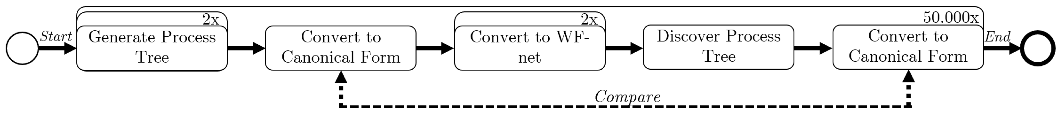
4.2. Experimental Setup

Here, we briefly discuss the experimental setup of our experiments. Consider Figure 13, in which we present a graphical overview. Using an implementation of PTandLogGenerator [18,19], we generate process trees, using two triangular distributions for the number of activities, i.e., $\{10,20,30\}$ and $\{40,50,60\}$. The process trees are translated to WF-nets, using two different translations. One translation creates invisible start and end transitions for each operator; the other translation only does so when required (similar to Figure 5). The first translation generates larger nets in terms of transitions/places/arcs. In general, the sizes of the respective WF-nets generated differs significantly.For each triangular distribution/translation combination, we generate $50.000$ process trees (yielding $200.000$ experiments). Finally, we compare the generated process tree in canonical form [20] [Section 5.1], to the resulting process tree in canonical form.

4.3. Results

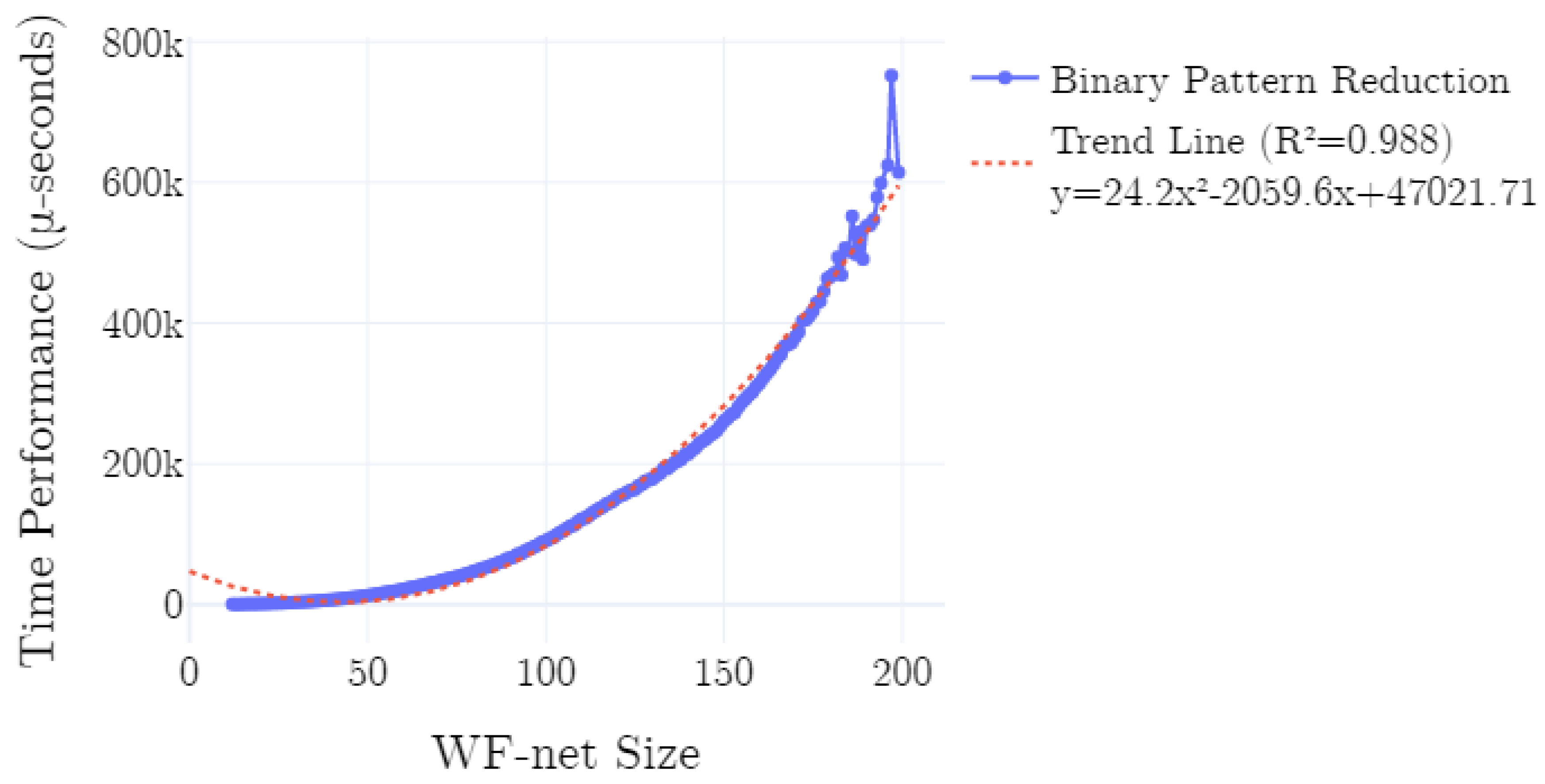
Here, we briefly discuss the results of the conducted experiments. Consider Figure 14, in which we present the average time performance of the implementation on the data as generated according to the described experimental setup. We plot the time performance, conditional to the size of the input WF-net. Additionally, we plot a polynomial trend-line, computed using polynomial least squares. As is clearly observable in Figure 14, the time performance is quadratic in the size of the net ($\left|P\right|+\left|T\right|$). This is confirmed by the $R^2$-score of the trend-line, i.e., ∼0.988. Note that, the fluctuations in the right-hand-side of the chart are explained by a relative smaller amount of experiments conducted with models of the corresponding sizes. In all experiments, the canonical form of the generated process tree equals the canonical form of the (re)discovered process tree.

5. Related Work

Process trees are often used in the domain of process mining. However, a complete overview of the field is outside of scope, i.e., we refer to [1] for a gentle introduction. Similarly, we refer to [21] for an in-depth overview of process discovery algorithms, and, we refer to [22] for an overview of the sub-field of conformance checking.

The conceptual idea of transforming a given process model in a certain formalism F into an alternative process modeling formalism $F^{\prime }$ is well-studied. Transformations of graph-oriented modeling formalisms, e.g., Petri nets, and block-oriented modeling formalisms, e.g., Process Trees, are often studied. In [10], the authors generalize work that transforms (both ways) graph-based process modeling formalisms into Business Process Execution Language for Webservices (BPEL) (an XML-based format). The authors characterize several strategies for such translations. In this context, the work presented in this paper belongs to the structure-identification category.

Of particular interest is the work of van der Aalst and Lassen [23,24], i.e., on translating of WF-nets to BPEL. In the work, XML fragments of BPEL are generated on the basis of a given WF-net. Since XML, by definition, is a tree-like data representation, BPEL and process trees are conceptually close. The algorithm replaces components, i.e., connected, complete subnets with a unique start and end element, i.e., such a start/end element can be either a place or a transition. The authors prove that “folding” a WF-net based on an identified component, under certain conditions, yields a sound WF-net. The folding operator for components as defined in [23] can be regarded as being very similar to the reduction (cf. Definition 9) presented in this paper. However, note that the proofs in [23] only hold for components, i.e., subnets with a single entry and exit. The algorithm described in [23] is similar to the algorithm presented in this paper, i.e., searching and replacing patterns until either a WF-net with a single transition is found, or no more pattern is found. However, within the algorithm, a specific ordering for the patterns and a maximization of the pattern-size is applied. Observe that, whereas the work in [23,24] is conceptually close to the work presented here, there are several differences as well. For example, in this work, we use system nets to represent patterns, i.e., lifting the single source/sink requirement for pattern recognition. As such, the algorithm presented in this paper is able to detect process tree fragments in WF-nets, in which the algorithm reported on in [23,24] would not find any fragments. Similarly, the algorithm presented in this paper does not impose any order on the reduction of the patterns identified, nor on their size. However, there is no clear motivation provided in [23] on the underlying reasons for imposing an order and maximization with respect to pattern detection.

In [25,26], the notion of the Refined Process Structure Tree (RPST) and its computation is introduced. The RPST is a hierarchical grouping of the edges present in a process model (defined as a workflow graph). As such, the given process model can be decomposed, i.e., on the basis of the hierarchy described by the RPST. Similar to the work in [23,24], the identified model-fragments need a single source and a single sink element. The works in [25,26] exemplify computing the RPST of a given BPMN model (which complies with the definition of the workflow graphs mentioned earlier), yet indicate that the concepts can be generalized to WF-nets. However, as we show in Section 6.2, the fact that the RPST, by definition, ignores the semantics of the model provided as an input leads the algorithm to find tree structures in unsound Workflow nets. The RPST decomposition has been exploited in various noteworthy other studies. In [27,28], the authors used the RPST to “structure acyclic process models”. The core idea is to compute an RPST decomposition of a given acyclic model, which is possibly unstructured. An unstructured part of the model is recognized as a rigid component in the RPST decomposition. Subsequently, the behavioral ordering relations of the rigid component are computed, and a corresponding structured process model is synthesized. Since there exist process models that do not have an equivalent well-structured representation, the aforementioned work is further extended in [29], in which the authors exploited the RPST decomposition to compute a maximally structured version of the input process model. In [30], the authors extended the notion of RPSTs for sound free-choice Wf-nets, i.e., referred to as a WF-tree. Within a WF-Tree, certain internal vertices can be labeled as being either place-bordered, transition-bordered, or as a loop construct. As such, the authors partially annotated the RPST with behavioral information. Whereas the RPST is computed on the basis of a tree of triconnected components, other similar tree-based abstractions of process models have been considered as well. In [31], the authors proposed to exploit the tree of biconnected components to check whether a given workflow net is sound on the basis of its structure. In particular, the authors show that it is sufficient to show that one biconnected subnet of the workflow net is not safe and sound, to conclude that the WF-net as a whole is not sound.

The reductions presented in this paper, alternatively to the different works on translating process modeling formalisms into each other, bear similarity to various reduction rules established on general Petri nets. The general idea of Petri net reduction (or the opposite, expansion) is a substitution of elements of a Petri net, i.e., either by a smaller or larger newly added subnet, while preserving the behavioral properties of the net. For example, in [32], the authors proposed step-wise refinements of both transitions and places in Petri nets, while preserving liveness and boundedness properties of the Petri net. Similarly, in [33], the author proposed a set of reduction rules for Colored WF-nets, i.e., WF-nets with additional data flow semantics. In [34], the authors presented a set of reduction rules for free-choice probabilistic WF-nets, i.e., WF-nets in which transitions have an associated probability and reward. In particular, the reduction rules are proposed in order to preserve the expected reward of the workflow.

Clearly, the work presented in this paper bears similarity with the different works mentioned. However, the works in the area of process model transformation are typically not defined for WF-nets, e.g., the RPST decomposition, or are more restrictive on the patterns to be replaced, e.g., the maximized unique source/sink patterns of [23]. Similarly, whereas the reduction patterns defined here do preserve the soundness of the WF-net, i.e., if the given WF-net is sound, the core of the related work in the field focuses more on the preservation of various behavioral properties.

6. Discussion

In this section, we discuss various aspects of the algorithm proposed in this paper. Firstly, in Section 6.1, we discuss the degree of extensibility of the framework, e.g., we discuss the detection of self-loops. Secondly, in Section 6.2, we provide an in-depth discussion of the relation of the proposed algorithm with respect to computation of the RPST decomposition. Finally, in Section 6.3, we discuss the reducibility of arbitrary WF-nets in the context of our proposed algorithm, i.e., we show an example of simple sound WF-nets for which the algorithm cannot find a corresponding process tree.

6.1. Extensibility

Since correctness of the proposed algorithm (cf. Theorem 1) holds for any feasible pattern (cf. Definition 8) that is globally language preserving, the algorithm presented in this paper is easily extended with additional reduction rules. Hence, any system net that describes a language that is equal to the language of a process tree can be reduced (conditional to the aforementioned global language preservation). For example, consider the self-loop reduction visualized in Figure 15.

Opposed to the other patterns presented and defined earlier, observe that, directly applying the reduction as defined in Definition 9, again yields a self-loop. Hence, in the reduction, we split-up the places, i.e., one group of places, forming the preset of the newly generated transition $t^{\prime }$ copies all incoming arcs of the places of the pattern (excluding the connections to $t_1,\dots ,t_2$). The other “freshly” added place copies all outgoing arcs of the places of the pattern (again excluding the connections to $t_1,\dots ,t_2$).

Consider Figure 16, in which we depict a simple example of the application of the self-loop reduction as described. The transitions $t_2$ and $t_3$ in the WF-net depicted in Figure 16a are self-loops on place $p_1$. In Figure 16b, the reduction is applied only on $t_2$. Note that, in this model, a loop reduction can be applied yielding $⥀(⥀(\tau ,b),c)$. Note that first reducing $t_3$ is symmetrical, i.e., eventually yielding $⥀(⥀(\tau ,c),b)$. Note that both process trees, indeed, describe the language ${(b^{*}{c}^{*})}^{*}$ (i.e., when described as a regular expression). In Figure 16c, we show the application of the self-loop reduction when it is applied directly using $T=\{t_2,t_3\}$. In this case, the reduction yields a new transition $t_2^{\prime }$ with label $⥀(\tau ,\times (b,c))$. Again, the language described by the process tree discovered can be described by ${(b^{*}{c}^{*})}^{*}$. Finally, let X denote any of the three process tree fragments discoverable in the example describing ${(b^{*}{c}^{*})}^{*}$. Observe that the reduction algorithm discovers $\to (a,X,d)$ (or any binary form thereof), which corresponds to the regular expression $a(b^{*}{c}^{*})d$, which is indeed the language of the WF-net depicted in Figure 16a.

Observe that the self-loop pattern shows that the algorithm proposed is extensible. However, in this case, the reduction step needs to be altered to avoid iteratively adding self-loop places (i.e., indefinitely). Any pattern can be reduced, as long as it is a feasible pattern that is globally language-preserving. For example, in some cases, the inclusive or operator is considered in the context of process trees, i.e., $\vee (Q_1,\dots ,Q_n)$. An inclusive or structure dictates that at least one of its children $Q_1,\dots ,Q_n$ is executed, yet, possibly, all are executed. The order in which the children are executed is irrelevant. Similarly, the interleaved operator is sometimes considered, i.e., $\leftrightarrow (Q_1,\dots ,Q_n)$. This operator requires that all its children are executed in any order, however, the behavior of the respective children cannot be shuffled, i.e., this is allowed by $\wedge (Q_1,\dots ,Q_n)$. Since both operators have a translation to a Petri net structure, these patterns can serve as a basis for reduction (potentially in a generalized form). However, note that these patterns are more involved with respect to the four basic patterns (and the self-loop pattern) presented in this paper.

6.2. Relation to Refined Process Structure Tree

One of the works that is conceptually very close to the work presented in this paper, is the work on the Refined Process Structure Tree (RPST) [25,26]. An RPST describes a hierarchy of sub-workflows of a workflow graph, such that each sub-workflow represents a connected subgraph with a single entry and single exit of control. In this context, a workflow graph is simply a two-terminal graph (TTG), i.e., a directed graph without self-loops with a unique source $(s)$ and sink node $(t\ne s)$, s.t. each node in the TTG is on a path from s to t. Note that a WF-net, i.e., from a graph-theoretical perspective, is a workflow graph. However, various other process modeling formalisms, e.g., BPMN, are also considered a workflow graph. Hence, an RPST can be computed on a much wider variety of process modeling formalisms, i.e., compared to the approach presented in this paper.

Formally, given a workflow graph $G_W=(V,E,w)$ (a multi-graph in which w assigns each edge in E to an ordered pair of nodes) an RPST is a hierarchy of fragments. A fragment is a subset $E^{\prime }\subseteq E$ of arcs, s.t., the subgraph formed by $E^{\prime }$ (including their incident vertices) is connected. Furthermore, the fragment should only contain one unique entry vertex and one unique exit vertex. A vertex is an entry vertex iff none of its incoming arcs are part of $E^{\prime }$ or all of its outgoing arcs are part of $E^{\prime }$. A vertex is an exit vertex iff none of its outgoing arcs are part of $E^{\prime }$ or all of its incoming arcs are part of $E^{\prime }$. The RPST of a workflow graph is the set of canonical fragments, i.e., those fragments that completely contain other fragments or are completely contained by other fragments, i.e., any overlap between fragments is not allowed. In [26], the authors showed that computation of an RPST is equivalent to computing the tree of triconnected components on a normalized variant of $G_W$ (normalization is performed by splitting vertices with multiple different incoming and outgoing edges into two nodes).

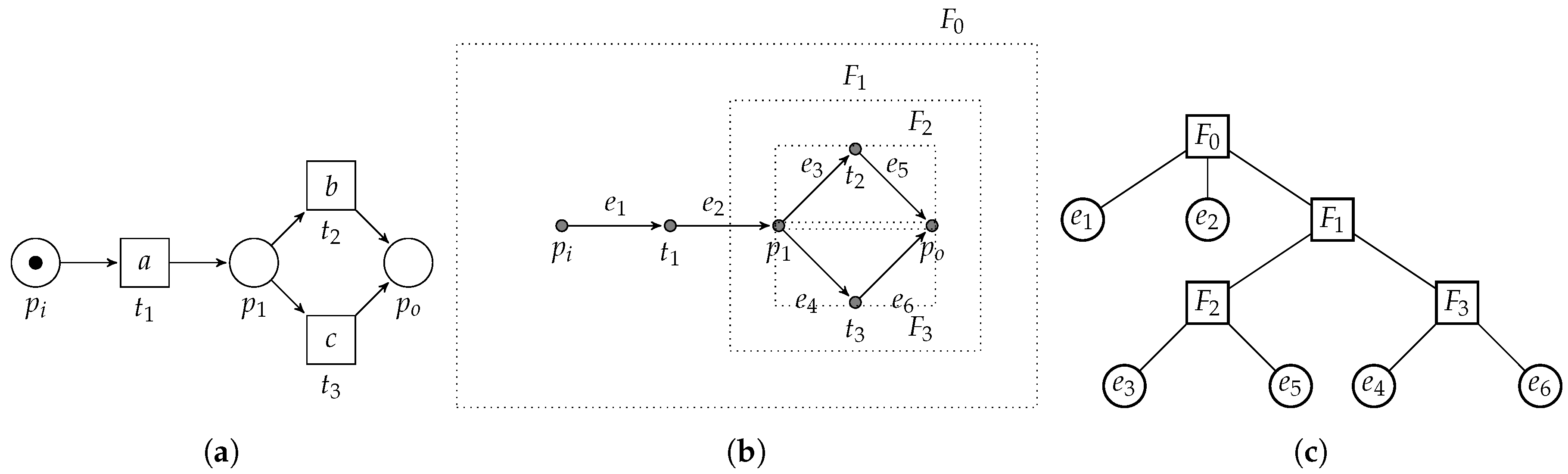
Clearly, each individual edge of a workflow graph is a fragment. Similarly, the complete set of arcs E defines a fragment. As an example, consider Figure 17, in which we present a simple example WF-net (Figure 17a) and its corresponding RPST decomposition (Figure 17b,c).

The edges $(p_i,t_1)$ and $(t_1,p_1)$, visualized as $e_1$ and $e_2$ are part of the root fragment, i.e., $F_0$, which is the complete edge set of the WF-net/workflow graph. The choice construct, i.e., connecting place $p_1$ and $p_o$ to transitions $t_2$ and $t_3$, respectively, comprises fragment $F_1$, which is further subdivided into fragments $F_2$ and $F_3$. Note that the process tree corresponding to $W_2$ is $\to (a,\times (b,c))$, i.e., consisting of 5 vertices. Hence, to translate the RPST to the corresponding process tree, we need to “collapse” $F_2$ and $F_3$ into b and c, respectively. Similarly, $F_1$ needs to be transformed to × and, $F_0$ needs to be transformed to →. Finally, $e_1$ and $e_2$ need to be merged into a.

The previous example illustrates that there is no general direct correspondence between the RPST of a WF-net and a corresponding process tree that describes the same language. Furthermore, it shows that translation of the RPST to a process tree is a non-trivial operation. As the RPST decomposition ignores the semantics of a WF-net, i.e., contributing to its more general applicability with respect to the algorithm presented in this paper (only applicable to process models that can be transformed into a WF-net), it also exists for WF-nets that are unsound.

Due to the generic nature of the RPST, i.e., it defines a graph-theoretical property of a workflow graph, it (largely) ignores the semantics and graph-theoretical properties of Petri nets. In particular, as an activity in a BPMN model only consists of a single entry and exit arc, within the underlying workflow graphs these activities are simply presented as a single edge. Since transitions in Petri nets represent process activities, and transitions are able to have multiple incoming and outgoing arcs, transitions in a WF-net cannot be represented as a single arc in the corresponding WF graph.

For example, consider Figure 18, in which we show the RPST of a WF-net that is not well-handled, i.e., $t_1$ generates concurrent behavior, place $p_3$ merges both branches of concurrent behavior. Since the RPST decomposition is not aware of the conceptual difference between places and transitions, the RPST subdivides the graph into several fragments. However, this is rather inconvenient, since the WF-net is not sound at all. Hence, from the RPST decomposition itself, one cannot judge whether a corresponding process tree exists.

The reverse is also possible, i.e., given a WF-net with a corresponding process tree representation, finding an RPST can be challenging. For example, when computing the RPST of the running example used in this paper, i.e., Figure 3, the behavior formed by the loop transition $t_6$ cannot be decomposed into smaller chunks (in terms of the RPST, the loop structure is generating a rigid fragment). Observe that the algorithm proposed in this paper is able to find the loop behavior due to the simplification of the reduction steps executed prior to the loop detection in Figure 6c.

Note that the aforementioned examples are not intended to disqualify the application of the RPST decomposition for the purpose of transforming WF-nets into process trees. However, they merely indicate that using the RPST decomposition as a basis for such translation is not a trivial adoption.

6.3. Reducibility of WF-Nets

Thus far, we have considered various system net based patterns that we reduce into a corresponding process tree notation. We have shown that, if the algorithm returns a WF-net with a specific structure, its label captures a process tree describing the same language as the original WF-net. However, it remains an open question what class of WF-nets are guaranteed to result in a process tree.

Since the basic operators considered in this paper all correspond to free-choice WF-nets, i.e., WF-nets s.t., $\forall p\in P\left(|p•|=1\vee •(p•)=\{p\}\right)$ (a place either has one outgoing arc, or it is the sole incoming arc of all transitions it connects to). Hence, intuitively, we suspect that the class of free choice nets always yields a corresponding process tree.

However, consider Figure 19, in which we depict a free-choice WF-net, which the proposed algorithm is not able to reduce.

Observe that the model consists of two concurrent branches, i.e., enabled by transition $t_1$. However, execution of transition $t_5$ is conditional to execution of $t_2$, i.e., firing both $t_3$ and $t_2$ enables transition $t_5$. One can look at this type of condition, i.e., induced by place $p_7$, as a non-local behavioral relation. There is interaction between members of the “upper part” and the “lower part” of the concurrent construct. Such a type of interaction cannot be modeled using a tree-based process modeling formalism.

Based on the previous example, we conclude that any class extending free-choice Petri nets might represent various WF-nets that cannot be reduced by the algorithm proposed. The notion of block-structured WF-nets seems to be an adequate subclass of free-choice WF-nets that can always be reduced by the model, i.e., they are often used interchangeable with process trees. However, an exact structural definition of the aforesaid class of WF-nets does not exist in the literature (yet). For example, in [20], an informal description of block-structured WF-nets is proposed: “A workflow net is block structured if for every place or transitions with multiple outgoing arcs, there is a corresponding place or transition with multiple incoming arcs. The parts of the net between the outgoing and incoming arcs form regions, and no arcs can exist between regions, i.e., the regions have a single entry and a single exit.” However, transforming this description into a formal, graph-theoretical property is not trivial for cyclic models.

7. Conclusions

In this paper, we present an algorithm to construct a process tree on the basis of a Workflow net (WF-net). The proposed algorithm replaces fragments of the WF-net that correspond to a process tree operator, i.e., by means of reduction rules. If the algorithm reduces the WF-net into a net, containing just one transition, there exists a corresponding process tree for the given WF-net, with the same language. The reduction rules proposed are bidirectionally soundness preserving. Hence, in the case a process tree is found, the original WF-net is sound. The contribution enables a wide variety of applications, e.g., improved computation performance of commonly used process mining artifacts, process model comparison and process model transformation. We conducted experiments using a prototypical implementation, indicating quadratic time complexity in the net and process tree rediscoverability.

Future Work We aim to extend the work presented in this paper in the following directions. We aim to provide diagnostics with respect to the reason a given WF-net cannot be reduced further, e.g., by assessing if removal of certain elements of the WF-net allows for further reduction. Alternatively, it is interesting to “wrap” certain fragments of the net into an encapsulating transition, after which the search to process tree fragments is continued. Another interesting direction, as briefly discussed in Section 6, is the search for structural properties of WF-nets that directly indicate whether a given WF-net corresponds to a process tree.

References

- van der Aalst, W.M.P. Process Mining—Data Science in Action, 2nd ed.; Springer: New York, NY, USA, 2016. [Google Scholar]
- Dijkman, R.M.; Dumas, M.; Ouyang, C. Semantics and analysis of business process models in BPMN. Inf. Softw. Technol. 2008, 50, 1281–1294. [Google Scholar] [CrossRef] [Green Version]
- van der Aalst, W.M.P. Formalization and verification of event-driven process chains. Inf. Softw. Technol. 1999, 41, 639–650. [Google Scholar] [CrossRef]
- van der Aalst, W.M.P.; Buijs, J.C.A.M.; van Dongen, B.F. Towards Improving the Representational Bias of Process Mining. In Proceedings of the SIMPDA, Campione d’Italia, Italy, 29 June–1 July 2011; pp. 39–54. [Google Scholar]
- Lee, W.L.J.; Verbeek, H.M.W.; Munoz-Gama, J.; van der Aalst, W.M.P.; Sepúlveda, M. Recomposing conformance: Closing the circle on decomposed alignment-based conformance checking in process mining. Inf. Sci. 2018, 466, 55–91. [Google Scholar] [CrossRef]
- van Zelst, S.J.; Bolt, A.; van Dongen, B.F. Computing Alignments of Event Data and Process Models. ToPNoC 2018, 13, 1–26. [Google Scholar]
- Schuster, D.; van Zelst, S.J.; van der Aalst, W.M.P. Alignment Approximation for Process Trees (forthcoming). In Proceedings of the 5th International Workshop on Process Querying, Manipulation, and Intelligence (PQMI 2020), Padua, Italy, 18 August 2020. [Google Scholar]
- van der Aalst, W.M.P.; de Medeiros, A.K.A.; Weijters, A.J.M.M. Process Equivalence: Comparing Two Process Models Based on Observed Behavior. In Proceedings of the Business Process Management, 4th International Conference, BPM 2006, Vienna, Austria, 5–7 September 2006; pp. 129–144. [Google Scholar]
- van Dongen, B.F.; Dijkman, R.M.; Mendling, J. Measuring Similarity between Business Process Models. In Seminal Contributions to Information Systems Engineering, 25 Years of CAiSE; Krogstie, J., Pastor, O., Pernici, B., Rolland, C., Sølvberg, A., Eds.; Springer: New York, NY, USA, 2013; pp. 405–419. [Google Scholar]
- Mendling, J.; Lassen, K.B.; Zdun, U. On the transformation of control flow between block-oriented and graph-oriented process modelling languages. IJBPIM 2008, 3, 96–108. [Google Scholar] [CrossRef]
- Berti, A.; van Zelst, S.J.; van der Aalst, W.M.P. Process Mining for Python (PM4Py): Bridging the Gap Between Process-and Data Science. In Proceedings of the ICPM Demo Track 2019, Aachen, Germany, 24–26 June 2019; pp. 13–16. [Google Scholar]
- Leemans, S.J.J.; Fahland, D.; van der Aalst, W.M.P. Discovering Block-Structured Process Models from Event Logs—A Constructive Approach. In Proceedings of the Application and Theory of Petri Nets and Concurrency—34th International Conference, Milan, Italy, 24–28 June 2013; pp. 311–329. [Google Scholar]
- Verbeek, E.; Buijs, J.C.A.M.; van Dongen, B.F.; van der Aalst, W.M.P. ProM 6: The Process Mining Toolkit. In Proceedings of the Business Process Management 2010 Demonstration Track, Hoboken, NJ, USA, 14–16 September 2010. [Google Scholar]
- van Dongen, B.F. BPI Challenge 2012; Eindhoven University of Technology: Eindhoven, The Netherlands, 2012. [Google Scholar] [CrossRef]
- van der Aalst, W.M.P. The Application of Petri Nets to Workflow Management. J. Circuits Syst. Comput. 1998, 8, 21–66. [Google Scholar] [CrossRef] [Green Version]
- Murata, T. Petri nets: Properties, analysis and applications. Proc. IEEE 1989, 77, 541–580. [Google Scholar] [CrossRef]
- van der Aalst, W.M.P. Workflow Verification: Finding Control-Flow Errors Using Petri-Net-Based Techniques. In Proceedings of the Business Process Management, Models, Techniques, and Empirical Studies, Berlin, Germany, 19 April 2000; pp. 161–183. [Google Scholar]
- Jouck, T.; Depaire, B. PTandLogGenerator: A Generator for Artificial Event Data. In Proceedings of the BPM Demo Track 2016, Rio de Janeiro, Brazil, 21 September 2016; pp. 23–27. [Google Scholar]
- Jouck, T.; Depaire, B. Generating Artificial Data for Empirical Analysis of Control-flow Discovery Algorithms—A Process Tree and Log Generator. Bus. Inf. Syst. Eng. 2019, 61, 695–712. [Google Scholar] [CrossRef]
- Leemans, S. Robust Process Mining with Guarantees. Ph.D. Thesis, Department of Mathematics and Computer Science, Eindhoven University of Technology, Eindhoven, The Netherlands, 2017. [Google Scholar]
- Augusto, A.; Conforti, R.; Dumas, M.; Rosa, M.L.; Maggi, F.M.; Marrella, A.; Mecella, M.; Soo, A. Automated Discovery of Process Models from Event Logs: Review and Benchmark. IEEE Trans. Knowl. Data Eng. 2019, 31, 686–705. [Google Scholar] [CrossRef] [Green Version]
- Carmona, J.; van Dongen, B.F.; Solti, A.; Weidlich, M. Conformance Checking—Relating Processes and Models; Springer: New York, NY, USA, 2018. [Google Scholar]
- van der Aalst, W.M.P.; Lassen, K.B. Translating unstructured workflow processes to readable BPEL: Theory and implementation. Inf. Softw. Technol. 2008, 50, 131–159. [Google Scholar] [CrossRef]
- Lassen, K.B.; van der Aalst, W.M.P. WorkflowNet2BPEL4WS: A Tool for Translating Unstructured Workflow Processes to Readable BPEL. In Proceedings of the CoopIS, DOA, GADA, and ODBASE, OTM Confederated International Conferences, Montpellier, France, 29 October–3 November 2006; pp. 127–144. [Google Scholar]
- Vanhatalo, J.; Völzer, H.; Koehler, J. The refined process structure tree. Data Knowl. Eng. 2009, 68, 793–818. [Google Scholar] [CrossRef]
- Polyvyanyy, A.; Vanhatalo, J.; Völzer, H. Simplified Computation and Generalization of the Refined Process Structure Tree. In Proceedings of the WS-FM 2010, Hoboken, NJ, USA, 16–17 September 2010; pp. 25–41. [Google Scholar]
- Polyvyanyy, A.; García-Bañuelos, L.; Dumas, M. Structuring Acyclic Process Models. In Proceedings of the Business Process Management—8th International Conference, Hoboken, NJ, USA, 13–16 September 2010; pp. 276–293. [Google Scholar]
- Polyvyanyy, A.; García-Bañuelos, L.; Dumas, M. Structuring acyclic process models. Inf. Syst. 2012, 37, 518–538. [Google Scholar] [CrossRef]
- Polyvyanyy, A.; García-Bañuelos, L.; Fahland, D.; Weske, M. Maximal Structuring of Acyclic Process Models. Comput. J. 2014, 57, 12–35. [Google Scholar] [CrossRef] [Green Version]
- Weidlich, M.; Polyvyanyy, A.; Mendling, J.; Weske, M. Causal Behavioural Profiles—Efficient Computation, Applications, and Evaluation. Fundam. Inform. 2011, 113, 399–435. [Google Scholar] [CrossRef] [Green Version]
- Polyvyanyy, A.; Weidlich, M.; Weske, M. The Biconnected Verification of Workflow Nets. In Proceedings of the On the Move to Meaningful Internet Systems: OTM 2010—Confederated International Conferences: CoopIS, IS, DOA and ODBASE, Hersonissos, Crete, Greece, 25–29 October 2010; pp. 410–418. [Google Scholar]
- Suzuki, I.; Murata, T. A Method for Stepwise Refinement and Abstraction of Petri Nets. J. Comput. Syst. Sci. 1983, 27, 51–76. [Google Scholar] [CrossRef] [Green Version]
- Esparza, J.; Hoffmann, P. Reduction Rules for Colored Workflow Nets. In Proceedings of the Fundamental Approaches to Software Engineering—19th International Conference, FASE 2016, Held as Part of the European Joint Conferences on Theory and Practice of Software, Eindhoven, The Netherlands, 2–8 April 2016; pp. 342–358. [Google Scholar]
- Esparza, J.; Hoffmann, P.; Saha, R. Polynomial analysis algorithms for free choice Probabilistic Workflow Nets. Perform. Evaluation 2017, 117, 104–129. [Google Scholar] [CrossRef] [Green Version]
Figure 1.
A simple example process tree [1], describing all basic control-flow constructs.
Figure 2.
The same process model, obtained by applying the Inductive Miner [12] implementation of ProM [13] on a real event dataset [14], in different process modeling formalisms. Because of its hierarchical nature, the process tree formalism easily allows us to spot the main control-flow behavior. (a) The process, represented as a WF-net; (b) The process, represented as a process tree.
Figure 3.
WF-net [1] with initial marking and final marking .
Figure 4.
Process tree [1], describing the same language as the WF-net in Figure 3 (reprint of Figure 1).
Figure 5.
Instantiations of (5). The -functions for operators are defined recursively, using the -values of their children, i.e., a place “entering”/“exiting” a fragment, connects to / (respectively) of .
Figure 6.
Application of the algorithm on the running example, i.e., . The label of , i.e., , depicted in Figure 6e, is the resulting process tree. The resulting process tree, i.e., , is equal to Figure 4. (a) Result of the first two rounds of the algorithm. The first two patterns that can be found are choice constructs, between b and c and between g and h, respectively. (b) Result of the third round of the algorithm on the running example. We find a concurrent construct between transition and . (c) Result of the fourth round of the algorithm. We find a sequential construct. (d) Result of the fifth round of the algorithm. We find a loop construct. (e) Result of the final round of the algorithm. We find a sequence construct.
Figure 7.
Example WF-net (and a corresponding reduction) in which we are able to detect the feasible pattern . The language of the original net (Figure 7a) is . The language of the reduced net (Figure 7b) is . Applying the label functions on the firing sequences yields different labeled languages. (a) A WF-net describing concurrent behavior between a sequential construct between a and c and activity b. Observe that the fragment formed by , , , , and is a feasible sequence pattern. (b) The (PTree)WF-net after reduction of the sequential pattern between , and .
Figure 8.
Example WF-net (and a corresponding reduction) in which we are able to detect feasible patterns ( and ) that are not globally language preserving. In the exemplary reduced net (Figure 8b), once we have executed , we are only able to execute the loop construct between , and . (a) The WF-net containing two local language equivalent feasible patterns. (b) The (PTree)WF-net after reduction of the loop pattern between , and .
Figure 9.
Schematic visualization of the →-pattern reduction (dashed arcs are allowed to be part of the pattern, solid arcs are required). The post-set of each transition acts as the pre-set of (). The transition replacing the identified pattern inherits and (these corresponding places are not explicitly visualized in this figure). The label of is formed by the sequence operator defined on top of the labels of , respectively.
Figure 10.
Visualization of the ×-pattern reduction (dashed arcs are allowed to be part of the pattern, while solid arcs are required). All transitions in the pattern share the same pre- and post-set. The replacing transition inherits the aforesaid pre- and post-set.
Figure 11.
Visualization of the ∧-pattern reduction. Transitions have disjunct pre-sets, yet, their pre-sets have the exact same pre-sets. The same holds for the post-sets of transitions . The replacing transition inherits all pre- and post-sets of .
Figure 12.
Visualization of the ⥀-pattern reduction. The pre-set of transition equals the post-set of and vice versa. The replacing transition inherits the pre- and post-set of transition .
Figure 13.
Overview of the experimental setup of the conducted experiments.
Figure 14.
Average time performance of the implementation. A quadratic relation, in computation time measured in micro-seconds (-seconds), with respect to the size of the WF-net, is observable.
Figure 15.
Schematic visualization of the -pattern reduction. The pre- and post-set of transitions are the same. In the reduction, the places are “split” into two groups, one copying all dashed incoming arcs, one copying all dashed outgoing arcs. The newly added transition is placed in between with label .
Figure 16.
Example application of the self-loop pattern reduction. (a) Simple WF-net, having self loop transitions , and . (b) Self-loop reduction where . (c) Self-loop reduction where .
Figure 17.
Example of an RPST decomposition (Figure 17c) based on the workflow graph (Figure 17b) of a simple sound WF-net (Figure 17a). (a) Simple WF-net . (b) The workflow graph of , including its canonical fragments. (c) The RPST of .
Figure 18.
Example of an RPST decomposition (Figure 18c) based on the workflow graph (Figure 18b) of a simple sound WF-net (Figure 18a). (a) Simple unsound (not well-handled) WF-net . (b) The workflow graph of , including its canonical fragments. (c) The RPST of .
Figure 19.
A Free-Choice WF-net for which the algorithm cannot find a corresponding process tree.
Publisher’s Note: MDPI stays neutral with regard to jurisdictional claims in published maps and institutional affiliations. |
© 2020 by the authors. Licensee MDPI, Basel, Switzerland. This article is an open access article distributed under the terms and conditions of the Creative Commons Attribution (CC BY) license (http://creativecommons.org/licenses/by/4.0/).
Share and Cite
MDPI and ACS Style
van Zelst, S.J.; Leemans, S.J.J. Translating Workflow Nets to Process Trees: An Algorithmic Approach. Algorithms 2020, 13, 279. https://0-doi-org.brum.beds.ac.uk/10.3390/a13110279
AMA Style
van Zelst SJ, Leemans SJJ. Translating Workflow Nets to Process Trees: An Algorithmic Approach. Algorithms. 2020; 13(11):279. https://0-doi-org.brum.beds.ac.uk/10.3390/a13110279
Chicago/Turabian Stylevan Zelst, Sebastiaan J., and Sander J. J. Leemans. 2020. "Translating Workflow Nets to Process Trees: An Algorithmic Approach" Algorithms 13, no. 11: 279. https://0-doi-org.brum.beds.ac.uk/10.3390/a13110279
Note that from the first issue of 2016, this journal uses article numbers instead of page numbers. See further details here.