
Cross-Entropy Method in Application to the SIRC Model


Faculty of Pure and Applied Mathematics, Wrocław University of Science and Technology, Wybrzeże Wyspiańskiego 27, 50-370 Wrocław, Poland
*
Authors to whom correspondence should be addressed.
Algorithms 2020, 13(11), 281; https://0-doi-org.brum.beds.ac.uk/10.3390/a13110281
Submission received: 23 September 2020
/
Revised: 27 October 2020
/
Accepted: 2 November 2020
/
Published: 6 November 2020
(This article belongs to the Special Issue Algorithms for Sequential Analysis)
Abstract
:The study considers the usage of a probabilistic optimization method called Cross-Entropy (CE). This is the version of the Monte Carlo method created by Reuven Rubinstein (1997). It was developed in the context of determining rare events. Here we will present the way in which the CE method can be used for problems of optimization of epidemiological models, and more specifically the optimization of the Susceptible–Infectious–Recovered–Cross-immune (SIRC) model based on the functions supervising the care of specific groups in the model. With the help of weighted sampling, an attempt was made to find the fastest and most accurate version of the algorithm.
Keywords:
optimal stopping; counting process; cross-entropy method; epidemiological models; SIR and SIRC models; cross-immunity and boostingMSC:
Primary: 90C59; Secondary: 49N90; 92D30; 68Q60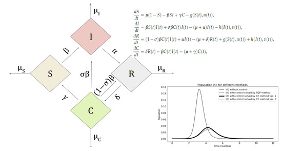
1. Introduction
In this study our aim is to develop the possibilities of numerically solving variational problems that appear in epidemic dynamics models. The algorithm that we will use for this purpose will be a modified Monte Carlo method. In a few sentences, we recall those stages of the Monte Carlo method development and its improvement, which constitute the essence of the applied approach (cf. Section 1.1 of Martino et al. [1]).
Before constructing the computer, the numerical analysis of deterministic models used approximations that aimed, among other things, at reducing and simplifying the calculations. The ability to perform a significantly larger number of operations in a short time led Ulam (cf. Metropolis [2]) to the idea of transforming a deterministic task to an appropriate stochastic task and applying the numerical analysis using the simulation of random quantities of the equivalent model (cf. Metropolis and Ulam [3]). The problem Ulam was working on was part of a project headed by von Neumann, who accepted the idea, and Metropolis gave it the name of the Monte Carlo Method [1] (in Section 1.1).
The resulting idea allowed one to free oneself from difficult calculations, replacing them with a large number of easier calculations. The problem was the errors that could not be solved by increasing the number of iterations. Work on improving the method consisted of reducing the variance of simulated samples, which led to the development of the Importance Sampling (IS) method in 1956 (cf. Marshall [4]).
Computational algorithms in this direction are a rapidly growing field. Currently, the computing power of computers is already large enough to provide an opportunity to solve problems that cannot be solved analytically. However, some problems and methods still require a lot of power. A lot of research is devoted to finding or improving such methods. The development of this field is currently very important. There are many models describing current problems. Not all offer the possibility of an analytical solution. That is why various studies are appearing to find the best methods for accurate results. the cross-entropy method helps to realize IS and it may, among other things, be an alternative to current methods in problems in epidemiological models.
1.1. Sequential Monte Carlo Methods
The CE method was proposed as an algorithm for the estimation of probabilities of rare events. Modifications of cross-entropy to minimize variance were used for this by Rubinstein [5] in his seminal paper [5] in 1997. This is done by translating the “deterministic” optimization problem in the related “stochastic” optimization and then simulating a rare event. However, to determine this low probability well, the system would need a large sample and a long time to simulate.
1.2. Importance Sampling
Therefore, it was decided to apply the importance sampling (IS), which is a technique used for reducing the variance. The system is simulated using other parameter sets (more precisely, a different probability distribution) that helps increase the likelihood of this occurrence. Optimal parameters, however, are very often difficult to obtain. This is where the important advantage of the CE method comes in handy, which is a simple procedure for estimating these optimal parameters using an advanced simulation theory. Sani and Kroese [6] have used the cross-entropy method as the support of the importance sampling to solve the problem of the optimal epidemic intervention of HIV spread. The idea of his paper will be adopted to treat the Susceptible–Infectious–Recovered–Cross-immune (SIRC) models, which has a wide application to modeling the division of population to four groups of society members based on the resistance to infections (v. modeling of bacterial Meningitis transmission dynamics analyzed by Asamoah et al. [7], Vereen [8]). The result will be compared with an analytical solution of Casagrandi et al. [9].
1.3. Cross-Entropy Method
This part will contain information on the methods used in the paper. The cross-entropy method developed in [5] is one of the versions of the Monte Carlo method developed for problems requiring the estimation of events with low probabilities. It is an alternative approach to combinatorial and continuous, multi-step, optimization tasks. In the field of rare event simulation, this method is used in conjunction with weighted sampling, a known technique of variance reduction, in which the system is simulated as part of another set of parameters, called reference parameters, to increase the likelihood of a rare event. The advantage of the relative entropy method is that it provides a simple and fast procedure for estimating optimal reference parameters in IS.
Cross-entropy is the term from the information theory (v. [10,11] (Chapter 2)). It is a consequence of measuring the distance of the random variables based on the information provided by their observation. The relative entropy, a close idea to the cross-entropy, was first defined by Kullback and Leibler [12] as a measure of the distance (v. [11] ((1.6) on p. 9; Definition on Section 2.3 p. 19), [13]) for two distributions p, q and is known also as Kullback–Leibler distance. This idea was studied in detail by Csiszár [14] and Amari [15]. The application of this distance measure in the Monte Carlo refinements is related to a realization of the importance sampling technique.
The CE algorithm can be seen as a self-learning code covering the following two iterative phases:
- Generating random data samples (trajectories, vectors, etc.) according to a specific random mechanism.
- Updating parameters of the random mechanism based on data to obtain a “better” sample in the next iteration.
Now the main general algorithm behind the cross-entropy method will be presented on the examples.
1.4. Application to Optimization Problems
This section is intended to show how extensive the CE method is. The examples will show the transformation of the optimization problems to the Monte Carlo task of estimation for some expected values. The equivalent MC task uses the CE method. Other very good examples can be found in [16].
The first variational problem presented in this context is the specific multiple stopping model. Consider the so-called secretary problem (v. Ferguson [17] or the second author’s paper [18]) for multiple choice, i.e., the issue of selecting the best proposals from a finite set with at most k attempts. There is a set with N objects numbered from 1 to N. By convention, the object with the number 1 is classified as the best and the object with the number N as the worst. Objects arrive one at a time in random order. We can accept this object or reject it. However, if we reject an object, we cannot return. The task is to find such an optimal stopping rule that the sum of the ranks of all selected objects is the lowest (their value is then the highest). So we strive for a designation
Let be the rank of the selected object. The goal is to find a routine for which the value of for , is the smallest. More details are moved to Appendix A.1.
Next, the problem was transformed into the minimization of the mean of the sum of ranks. The details are presented in Appendix A.2. This problem and its solution by CE was described by Polushina [19]. Its correctness was checked and programmed in a different environment by Stachowiak [20].
The second example is presented in detail in Appendix A.3. It is a formulation of the vehicle routing problem (v. [21,22]). This is an example of stochastic optimization where the cross-entropy is used.
1.5. Goal and Organization of This Paper
In the following parts of the paper, we will focus on models of the dynamics of the spread of infection over time when the population consists of individuals susceptible to infection, sick, immune to vaccination or past infection, and partially susceptible i.e., the population is assigned to four compartments of individuals. Actions taken and their impact on the dynamics of the population are important. It is precisely the analysis of the impact of the preventive diagnosis and treatment that is particularly interesting in the model. How the mathematical model covers such actions is presented in Section 2.1. The model created in this way is then adapted for Monte Carlo analysis in Section 2.2 and the results obtained on this basis are found in Section 2.3. The analysis of computational experiments concludes this discussion in Section 3.
2. Optimization of Control for SIRC Model
Let us focus the attention on the introduction of SIRC model and presentation of the logic behind using the CE method to determine functions that optimize the spread of epidemics. The ideology behind the creation of the SIRC model and its interpretation will be presented in order to match the right parameters for calculating the cost functions.
The CE method here is used to solve the variational deterministic problem. Solving such problems has long been undertaken with the help of numerical methods with a positive result. In the position [23] proposals of the route for variational problems for optimization problems in time are presented. The main focus was on the non-convex problems, which often occur with optimal control problems. In the book by Glowinski [24] a review of the methods for solving variational problems was made. Then [25] presented a complicated method of approximating functions for the problem optimization.
2.1. SIRC Model
The subject of the work is to solve the problem of optimizing the spread of the disease, which can be modeled with the SIRC model. This model was proposed by Casagrandi et al. [9]. Its creation was intended to create a better model that would describe the course of influenza type A. Contrary to appearances, this is an important topic because the disease, although it is widely regarded as weak, is a huge problem for healthcare. In the US alone, the cost associated with the influenza epidemic in the season is estimated to exceed USD 10 billion (v. [26]) and the number of deaths is over 21,000 per season (v. [27]).
Various articles have previously proposed many different mathematical models to describe a pandemic of influenza type A. An overview of such models was made by Earn [28]. In general, it came down to combining SIR models with the use of cross-resistance parameters (cf. details in the papers by Andreasen et al. [29] and Lin et al. [30]). The authors of the article write that the main disadvantage of this approach is the difficulty of the analysis and calculations with a large number of strains. The results of their research showed that the classic SIR model cannot be used to model and study influenza epidemics. Instead, they proposed the extension of the SIR model to a new class C that will simulate a state between a susceptible state and a fully protected state. This extension aims to cover situations where vulnerable carriers are exposed to similar stresses as they had before. As a result, their immune system is stronger when fighting this disease.
The SIRC model divides the community into four groups:
- ▪
- S—persons susceptible to infection, who have not previously had contact with this disease and have no immune defense against this strain
- ▪
- I—people infected with the current disease
- ▪
- R—people who have had this disease and are completely immune to this strain
- ▪
- C—people partially resistant to the current strain (e.g., vaccinated or those who have had a different strain)
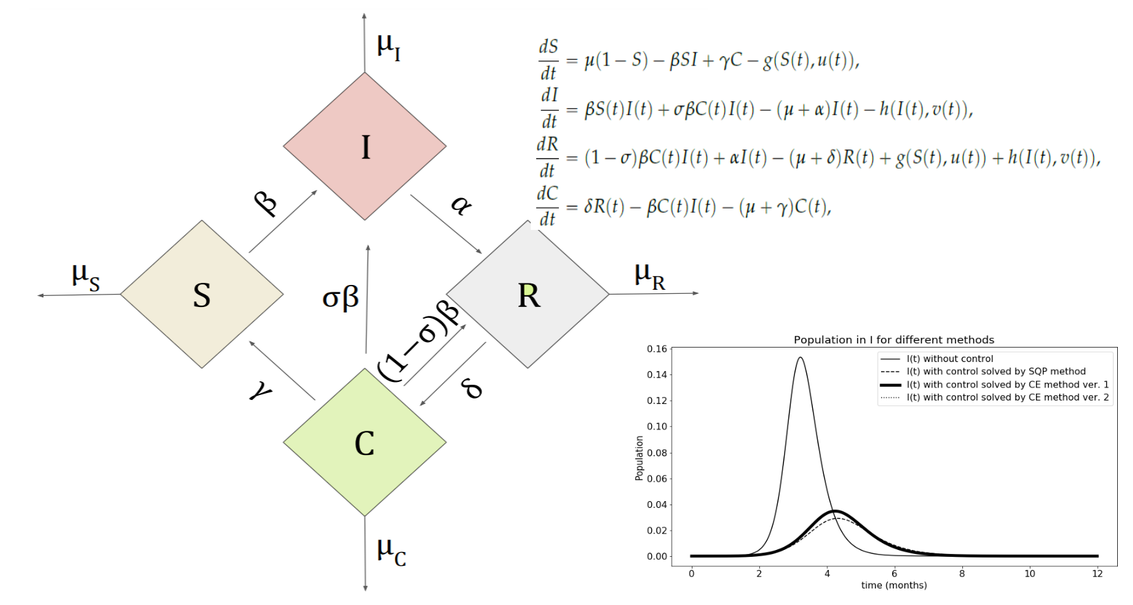
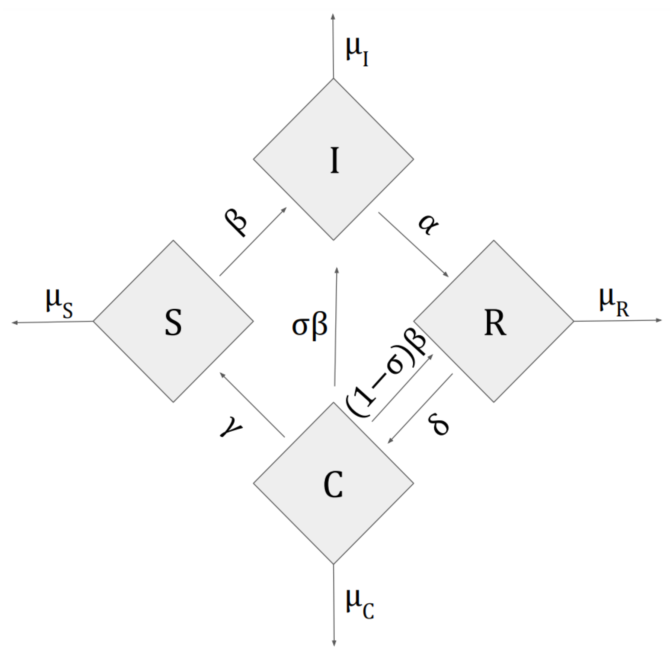
Figure 1 contains a general scheme of this model. The four rhombi represent the four compartments of individuals, the movement between the compartments is indicated by the continuous arrows. The main advantage of this model over other SIR users is the fact that after recovering from a given strain, in addition to being completely resistant to this strain, they are also partly immune to a new virus that will appear later. This allows you to model the resistance and response of people in the group to different types of diseases.
Parameters i can be interpreted as the reciprocal of the average time spent by a person in order of ranges . Parameters with indices represent the natural mortality in each group, respectively. In some versions of the model, additional mortality rates are considered for the group of infected people. Here we assume that this factor is not affected by the disease and we will denote it as in later formulas (). The next one is the likelihood of reinfection of a person who has cross-resistance while the parameter describes the contact indicator.
The SIRC model is represented as a set of four ordinary differential equations. Let , be the number of people in adequate compartments. We have (v. [9])
with initial conditions
2.2. Derivation of Optimization Functions
An approach to optimize this model was proposed by Iacoviello and Stasio [31]. In this article one can find the suggestion concerning performing the calculations as outlined by Zaman et al. [32]. Two functions were proposed in the approach as the parameter or controls. One relates to the susceptible people and the other describes the number of sick people. The method described by Kamien and Schwartz [33] was used to determine the optimal solution. In order to apply it, the set of Equation (1) should be updated accordingly. After these modifications, it has the following form:
where
where represent the percentage of those susceptible who have been taken care of thanks to using control on population and represent the percentage of infected people with the same description, respectively. and are weights that optimize the proportion of given control options. Both functions and in order they can be interpreted as actions performed on people susceptible to the disease and infected. In addition, two new conditions related to optimization functions are added to the initial conditions.
They describe the limits on what part of the population care can be given to. The smallest values and is zero. The existence of the solution is shown by Iacoviello et al. [31] and they are functions that minimize the following cost index:
are used to maintain the balance in the susceptible and infected group. is interpreted as weighting in the cost index. determine the time interval. The square next to the functions and indicates increasing intensity of functions [32]. Thus the function reflects the human value of susceptible and infected persons, taking into account the growing value of funds used over a specified period of time.
The objective function can be changed as long as there is a minimum. The CE method does not impose any restrictions here. However, to compare the results with [31], the function proposed by them is used also here. There, the objective function must be square in order for the quadratic programming techniques to be used. Usually, the quadratic function is good in mathematics, but not in practice. Changing the objective function and impact of it can be considered further.
2.3. Optimization of the Epistemological Model by the CE Method
Sani and Kroese [6] present the way in which the cross-entropy method can be used to solve the optimization of the epistemological model consisting of ordinary differential equations. The main task was to minimize the objective function depending on one optimization function over a certain set U consisting of continuous functions u. The minimum can be saved as:
Parameterizing the minimum problem looks as follows:
where is a function from U, which is parameterized by a certain control vector . Collection C is a set of vectors c. It should be noted that the selected set C should be big enough to get the enough precise solution. Then in such a set there are such —which will be the optimal control vector and —optimal value, respectively.
One way to parameterize a problem is to divide the time interval at small intervals and using these intervals together with control vector points c to define a function . This function can be created by interpolating between points. Such interpolation can be done using e.g., the finite element method, finite difference method, finite volume method or cubic B-Spline. Fang et al. [34] and Caglar et al. [35] show that all of this methods can be used to the two-point boundary value problems. Here the FEM method was used (v. [36]). The results for the other methods have not been checked. The choice of the approximation method is a difficult and interesting issue, but this is not what is consider here. With this function , it takes form
where
Now when is represented as a parameterized function, the value can be counted by solving the system of ordinary differential Equation (3) e.g., by the Runge–Kutta method. The idea of using the CE method in this problem is to use a multi-level algorithm with generated checkpoints , here, from a normal distribution. The CE method does not impose the distribution. Usually it is chosen from the family of density which is expected. Here, it is expected that there will be one high peak at the peak of the epidemic. Hence the normal distribution. Then, update the distribution parameters using the CE procedure using the target indicator as a condition for selecting the best samples. The calculations are carried out until the empirical variance of optimal control function is smaller than the given . This means that the function values are close to the optimal expected value The idea of applying the CE method to the SIRC model is similar. The only difficulty is the fact that when optimizing the SIRC model there are two functions instead of one as in the case of the algorithm described here. In the form of an Algorithm 1, it looks as follows:
| Algorithm 1: (Modification of the Sani and Kroese’s algorthm (v. [6]) to two optimal functions case): |
|
The value of the criterion is calculated in steps 3 and 4. The selection of the function allows us to fit the cost function to the modeled case. Here, the criterion given by (6) is adopted.
3. Description of the Numerical Results
This section will present the results obtained using the cross-entropy method. For the correct comparison the same parameters for the SIRC model were used. These values are:
For optimization functions and the following restrictions have been applied:
Restrictions were proposed by Lenhart and Workman [37]). Their value was explained by the fact that the whole group cannot be controlled. In addition, the weights used for functions have values and
Now, all that’s left is to propose variable values for the objective function:
The parameter values are adjusted using historical data like parameter mortality rate , which is counted as average lifetime of a host or parameters mean the inverted time of belonging to the group and C. A detailed description of determining parameters along with their limitations is presented in the article by Casagrandi et al. [9].
3.1. A Remark about Adjusting the Parameters of the Control Determination Procedure
Here these parameters are given and describe the influenza A epidemics well, because of long historical data sets. However, this may not be the case, and then these parameters are subject to adjustment in the control determination procedure. An overview of applications and accuracy of calibration methods, which can be used, is presented in the article by Hazelbag et al. [38], which provides an overview of the model calibration methods. All parameters in the model are constant and independent of time, so methods that try to optimize a goodness-of-fit (GOF) can be used for this example. GOF is a measure that assesses consistency between model the output and goals. As a result, it gives the best combination of parameters. Examples of such methods are grid search, Nelder–Mead method, the iterative, descent-guided optimization algorithm, sampling from a tolerable range. After finding the appropriate parameters, other algorithms like the profile likelihood method or Fisher information can be used to calculate the confidence intervals for these coefficients. If the epidemic described by the model consists of transition probabilities that cannot be estimated from currently available data, calibrations can be performed to many end points. Then GOF is measured as the mean percentage deviation of the values obtained at the endpoints (v. [39]).
3.2. Proposed Optimization Methods in the Model Analysis
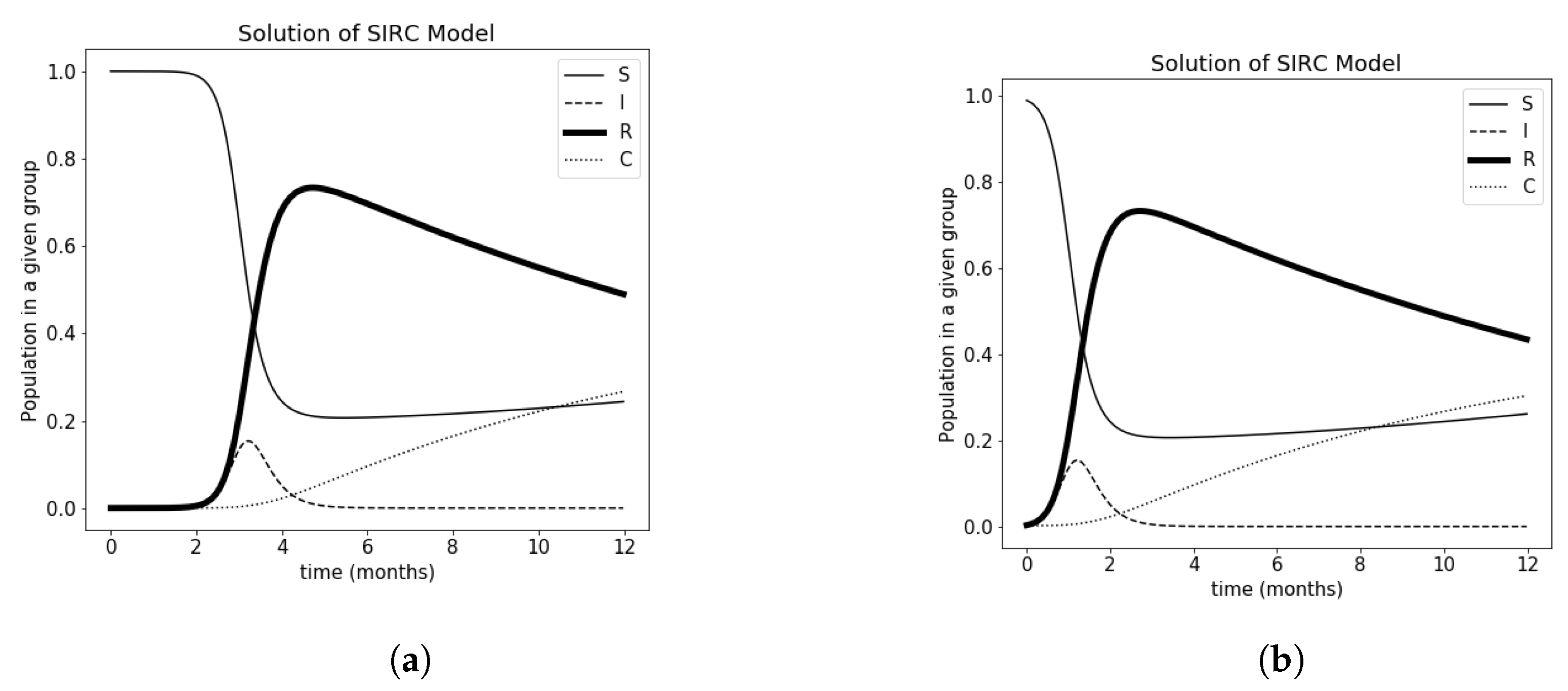
The results will be presented for two moments in the model: at the beginning and in the middle of the epidemic. This is initialized with other initial parameters. For the beginning of the epidemic, they are as follows:
For the widespread epidemic:
The values in the model have been normalized for the entire population, and they add up to 1. The results for both beginning (v. Figure 2a) and during (v. Figure 2b) the epidemic were obtained using the Runge-Kutty method and shown here. The cost index in this case was in order and for the model of the beginning and the development of an epidemic.
In Section 3.3 and Section 3.4 two ways of calculating optimal functions and for the SIRC model will be considered. In the first version, the functions will be calculated separately. In the following, both and will be counted at the same time. All versions will be presented at two moments of the epidemic: when it began and when it has already spread. The results will be compared with those obtained in the article by Iacoviello et al. [31], where the problem was solved using the sequential quadratic programming method using a tool from Matlab. Unfortunately, the article does not specify the cost index value for solving the obtained sequential quadratic programming method. Therefore, in the paper, there were attempts to recreate the form of the function and and the cost index obtained for them ( for the first situation and for the second one) and the model solution.
As can be seen in Figure 3 in the first situation, the control functions helped reduce peak infection, which was previously (without control Figure 2a) occurred between 2 and 4 months. The largest peak was around occurred between 2 and 4 months. Previously, the largest peak was around . In the case of the second situation, the peak also decreased, but not very clearly (it is also visible in the value of the cost index, which for the first situation is , and for the other one ). It can be seen that timely control is also very important to reducing the harmful effects of an epidemic. For more conclusions on how to apply control properly in this model, see [31].
3.3. CE Method Version 1
In the first method, the algorithm is shown at the end of Section 2.3 has been applied twice. Once for the calculation of the optimal function with a fixed , and then with a fixed . In the next step, the results were combined and the result for the SIRC model was calculated using these two functions. This approach is possible due to the lack of a combined restriction on and . Features are not dependent on each other with resources.
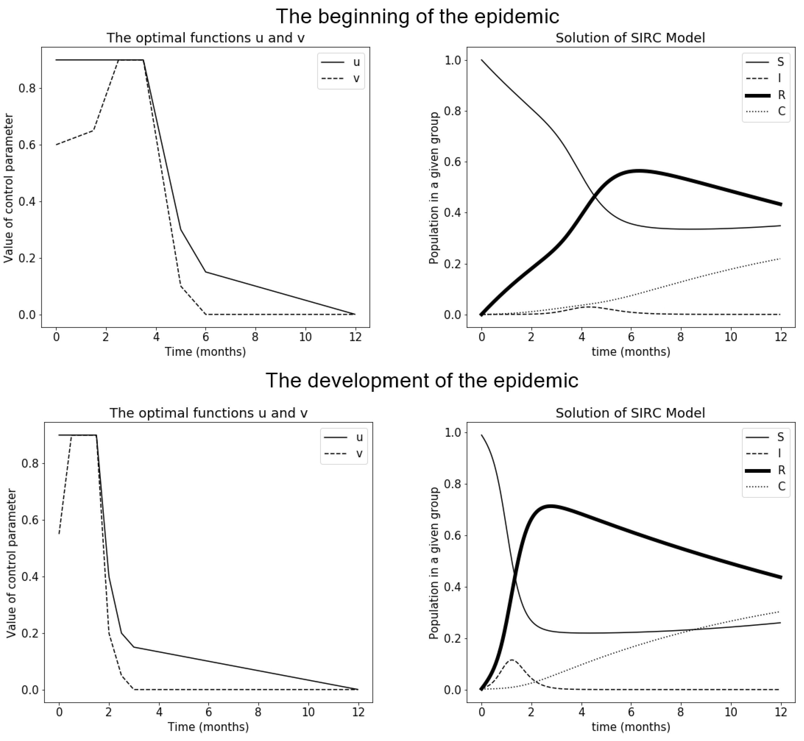
The cost index was for the start of the epidemic and for a developed epidemic. The Figure 4 show the graphs of functions and along with a graph of solutions for both moments during the epidemic.
For functions the results are similar, only the decrease here is more linear. However, the solution of the SIRC model gives the same results. Function is much more interesting. The CE method showed that it should have very low values, even close to 0 throughout the entire period in both cases. However, this does not affect the cost index (it is even smaller than in the previous case) and the SIRC model. More on this subject will be included in the summary.
3.4. CE Method Version 2
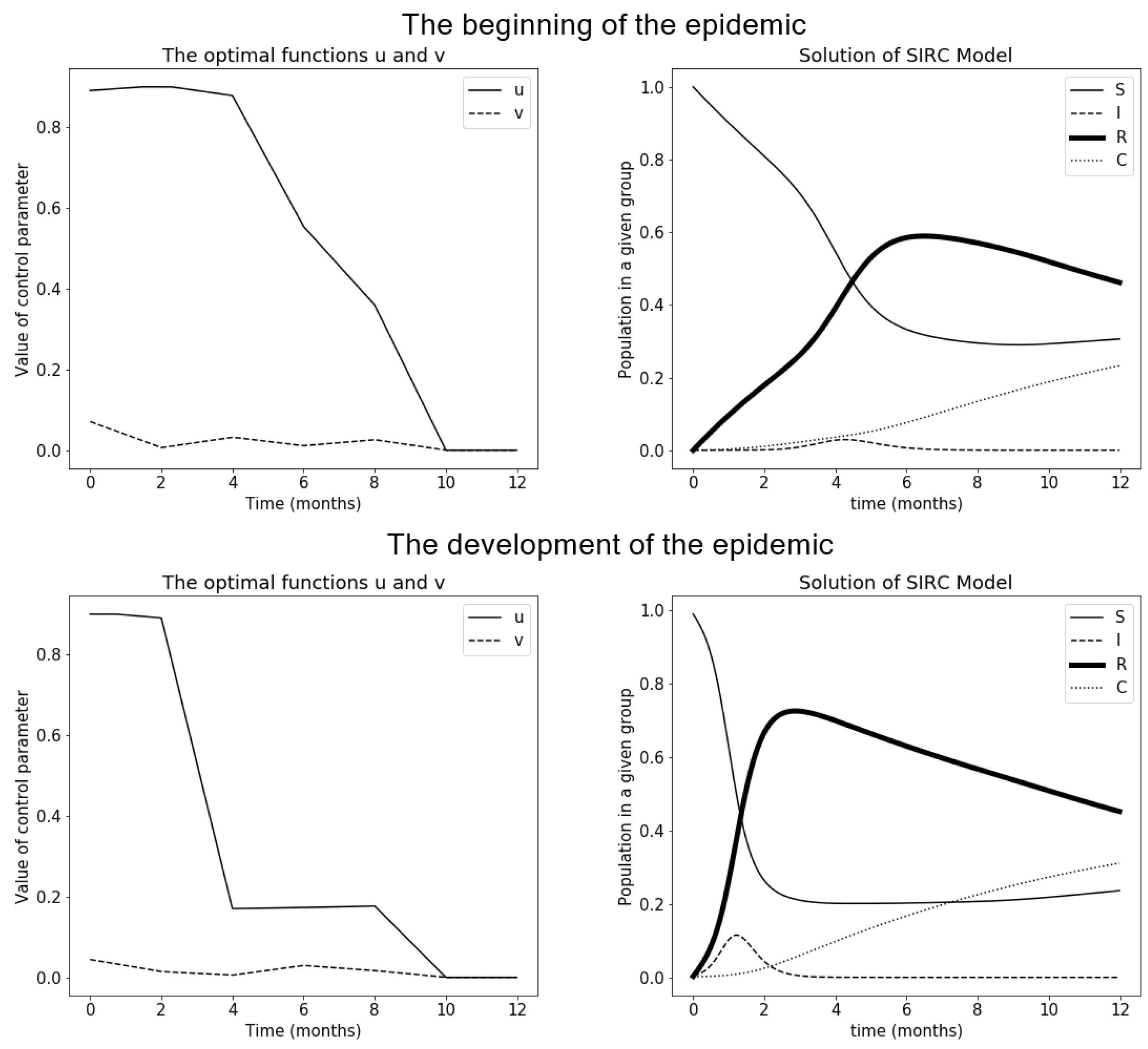
In the second case, it was necessary to change slightly the algorithm from Section 2.3 to be able to use it for two control functions. In point 1 of the algorithm a variable is generated , which serves to designate , where are requested by the user. Here, 2 will need to be initialized and 2 : . Then designate and similarly . Now can be count without problems. Further the algorithm goes the same way, and in point 6, all four parameters are updated. The Figure 5 presents these functions.
In this case, we have very similar results as in the previous section. This can be seen in both the charts and the cost index values ( and ). The only problem here is the need for a large sample to bring the results closer.
3.5. Comparison of Results
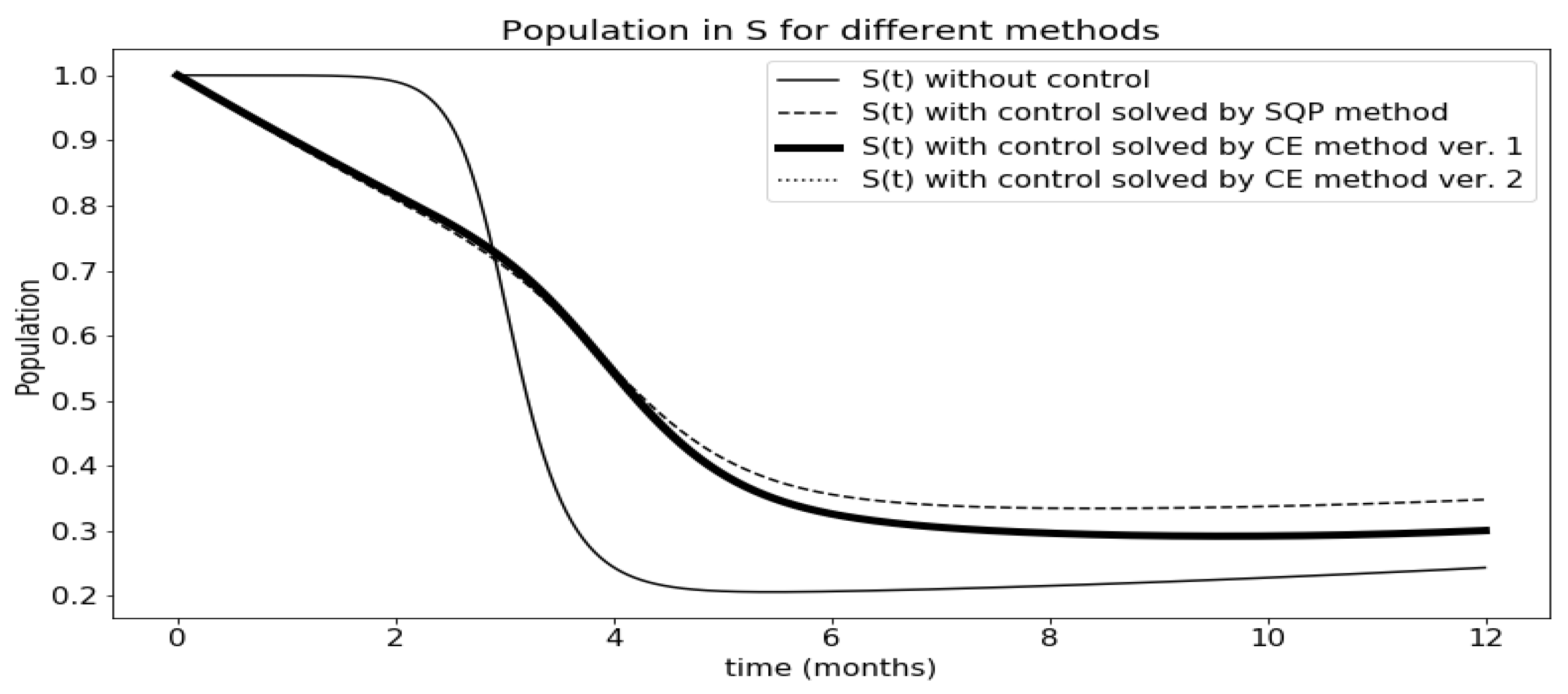
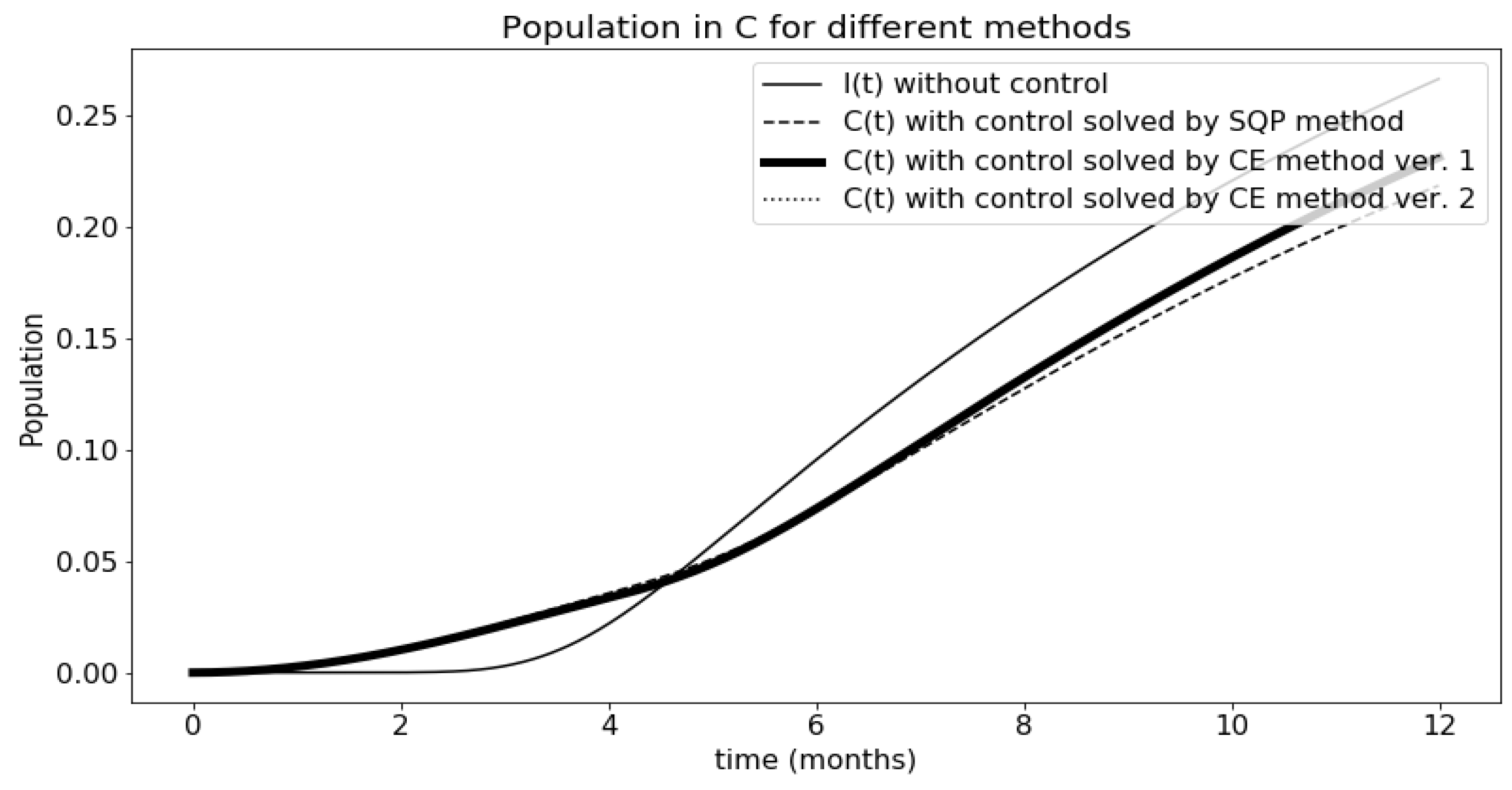
This section gathers the results from each version and compares them with each other. At first, the behavior of each group of the SIRC model was looked at and compared with the solution of the uncontrolled model. This is shown in Figure 6, Figure 7, Figure 8 and Figure 9. The results are presented only for the first situation, where the epidemic begins to spread, because there you can see the results of using control much better.
The most interesting is Figure 7 comparing infected people. You can see here very well how functions and help in the fight against the epidemic. Let two versions of the CE method overlap. The functions obtained by the sequential quadratic programming method give slightly better results. However, they have a worse cost index (the comparison is presented in Table 1). This is probably due to the high value of the function , which increases the cost index. The question remains why there is such a discrepancy between the obtained function values with both methods. In this article [31] weight and impact of functions and were compared. The chart in the article compares the results obtained for the application of both functions, one at a time and none. It turned out that the main influence on the number of infected has control over susceptible persons, i.e., the function . Choosing the optimal values for is not very important for the solution of the model. Therefore, such discrepancies are possible when choosing optimal values.
Table 1 contains a comparison of the cost index values and the duration of the algorithms for each method. The first value is when the epidemic started, and the second is when it has already developed. The article does not specify the algorithm time of the method used.
It can be seen that for each version the cost index values came out very similar. The differences can be seen in time. This is because in the first version of the CE method a smaller sample was simulated because both functions were considered separately. Fortunately, the functions were not closely related and it was possible to consider them separately.
4. Summary
The study examined the possibility of using the CE method to determine the optimal control in the SIRC model. Similar models are being developed to model the propagation of malicious software in computer networks (v. Taynitskiy et al. [40]). However, the number of works with this approach is still relatively small, although its universality should encourage checking its effectiveness. There are two control functions in the model, which, when properly selected, optimize the cost function. The CE method was used in two versions: considering the two functions separately and together. The results were then compared with those obtained by Iacoviello and Stasio [31] using routing of Matlab (Matlab is a paid environment with a number of functions. Unlike other environments and programming languages, additional features are created by developers in a closed environment and can only be obtained through purchase.). The Cross-Entropy method had little problems when considering two functions at the same time. Due to the large number of possibilities, it was necessary to simulate a large sample, which significantly extended the algorithm’s time. The second way came out much better. However, it only worked because the functions were not dependent on each other. In the opposite situation, there is also a possibility to get the result via CE results however, it will be necessary to change the algorithm and the dependence of how the functions depend on each other and add this to the algorithm when initiating optimization functions in the code. The same situation applies to changing the objective function and the density used for approximation. Changing the objective function gives the possibility to use other methods. If it stays quadratic and the constraints are linear, quadratic programming techniques like the sequential quadratic programming method can still be used. If the objective function and the constraints stay convex, we use general methods from convex optimization. The CE method is based on well-known and simply classical rules and is therefore quite problem-independent. There are no rigid formulas, and therefore it requires consideration for each problem separately. So it is very possible to reconsider it in another way, which can be interesting for further work. The CE method may also facilitate the analysis of modifications of epidemiological models related to virus mutation or delayed expression (v. Gubar et al. [41], Kochańczyk et al. [42]).
Author Contributions
K.J.S. gave an idea of application of CE to SIRC model; M.K.S. realized implementation and simulation. All authors have read and agreed to the published version of the manuscript.
Funding
K.J.S. are thankful to Faculty of Pure and Applied Mathematics for research funding.
Conflicts of Interest
The authors declare no conflict of interest.
Abbreviations
The following abbreviations are used in this article:
| CE | Cross-entropy method (v. page 2) |
| FEM | the finite element methods (v. page 6) |
| GOF | a goodness-of-fit (v. page 8) |
| IS | the importance sampling (v. page 2) |
| SIR | The SIR model is one of the simplest compartmental models. The letters means the number of Susceptible–Infected–Removed (and immune) or deceased individuals. (v. [43,44,45,46]). |
| SIRC | The SIR model with the additional group of partially resistant to the current strain people: Susceptible–Infectious–Recovered–Cross-immune (v. page 4). |
Appendix A. Optimization by the Method of Cross-Entropy
Appendix A.1. Multiple Selection to Minimize the Sum of Ranks
Let be a permutation of integers , where all permutations are equally probable. For every will be the number of values , which are . is the relative rank of the i-th object. The decision-maker observe the relative ranks and the real ranks define filtration: . Let be the set of Markov time with respect to . Define
We want to find the optimal procedure and the value of the optimization problem v. Let be -algebra generated by . If we accept
then
The problem is reduced to the problem of stopping sequences multiple times . As shown in [47,48] the solution to the problem is the following strategy:
If there are integer vectors
then
on the set . , . For small N there is a possibility to get accurate values by the analytical method. The CE method solves this problem by changing the estimation problem to the optimization problem. Then by randomizing this problem using a defined family of probability density functions. With this the CE method solves this efficiently by making adaptive changes to this pdf and go in the direction of the theoretically optimal density.
Appendix A.2. Minimization of Mean Sum of Ranks
Let’s consider the following problem of minimizing the mean sum of ranks:
where conditions from (A1) are preserved} is some defined set. is a random permutation of numbers . is an unbiased estimator with the following formula:
where is the nth copy of a random permutation R.
Now, a cross-entropy algorithm can be applied (v. Section 1.3 and [5]). Let’s define the indicator collections on for different levels . Let be the density family on parameterized by the actual parameter value u. For a specific u we can combine (A2) with the problem of estimation
where is a measure of the probability in which the random state X has a density and is a known or unknown parameter. l we estimate using the Kullback–Leibler distance. The Kullback–Leibler distance is defined as follows:
Usually is chosen from the family of density . So here D for g and it comes down to selecting such a reference parameter v for which is the smallest, that is, it comes down to maximization:
After some transformations:
So firstly, let us generate a pair , which we then update until the stopping criterion is met and the optimal pair is obtained . More precisely, arrange and choose not too small and we proceed as follows:
- (1)
- Updating Generate a sample from . Calculate and sort in ascending order. For choose
- (2)
- Updating obtain from the Kullback–Leibler distance, that is, from maximizationsoAs in [49], here a three-dimensional matrix of parameters is consider.It seems thatand then after some transformationswhere , is a random variable from , corresponding to the Formula (A4). Instead of updating a parameter use the following smoothed version
- (3)
- Stopping Criterion The criterion is from [16], which stop the algorithm when (T is last step) has reached stationarity. To identify the stopping point of T, consider the following moving average processwhere K is fixed.Then let us defineandwhere R is fixed.Then the stopping criterion is defined as followswhere K and R are fixed and is not too small.
Appendix A.3. The Vehicle Routing Problem
The classical vehicle-routing problem (VRP) is defined on a graph , where is a set of vertices and , is the arc set. A matrix can be defined on , where the coefficient defines the distance between the nodes and and is proportional to the cost of travelling by the corresponding arc. There can be one or more vehicles starting off from the depot with a given capacity, visiting all or a subset of the vertices, and returning to the depot after having satisfied the demands at the vertices. The Stochastic Vehicle Routing Problem (SVRP) arises when elements of the vehicle routing problem are stochastic—the set of customers visited, the demands at the vertices, or the travel times.
Let us consider that a certain type of a product is distributed from a plant to N customers, using a single vehicle, having a fixed capacity Q. The vehicle strives to visit all the customers periodically to supply the product and replenish their inventories. On a given periodical trip through the network, on visiting a customer, an amount equal to the demand of that customer is downloaded from the vehicle, which then moves to the next site. The demands of a given customer during each period are modeled as independent and identically distributed random variables with known distribution. A reasonable assumption is that all the customers’ demands belong to a certain distribution (say normal) with varying parameters for different customers.
The predominant approach for solving the SVRP class of problems is to use a “here-and-now” optimization technique, where the sequence of customers to be visited is decided in advance. On the given route, if the vehicle fails to meet the demands of a customer, there is a recourse action taken. The recourse action could be in the form of going back to the depot to replenish and fulfill the customers’ demand continue with the remaining sequence of the customers to be visited or any other meaningful formulation. The problem then reduces to a stochastic optimization problem where the sequence with the minimum expected distance of travel (or equivalently, the minimum expected cost) has to be arrived at. The alternative is to use a re-optimization strategy whereupon failure at a node, the optimum route for the remaining nodes is recalculated. The degree of re-optimization varies. At one extreme is the use of a dynamic approach where one can re-optimize at any point, using the newly obtained data about customer demands, or to re-optimize after failure. Neuro Dynamic Programming has been used to implement techniques based on re-optimization (cf. e.g., [50]).
The vehicle departs at constant capacity Q and has no knowledge of the requirements it will encounter on the route, except for the probability distributions of individual orders. Hence, there is a positive probability that the vehicle runs out of the product along the route, in which case the remaining demands of that customer and the remaining customers further along the route are not satisfied (a failure route). Such failures are discouraged with penalties, which are functions of the recourse actions taken. Each customer in the set can have a unique penalty cost for not satisfying the demand. The cost function for a particular route traveled by the vehicle during a period is calculated as the sum of all the arcs visited and the penalties (if any) imposed. If the vehicle satisfies all the demands on that route, the cost of that route will simply be the sum of the arcs visited including the arc from the plant to the first customer visited, and the arc from the last customer visited back to the plant.
Alternatively, if the vehicle fails to meet the demands of a particular customer, the vehicle heads back to the plant at that point, terminating the remaining route. The cost function is then the sum of all the arcs visited (including the arc from the customer where the failure occurred back to the plant) and the penalty for that customer. In addition, the penalties for the remaining customers who were not visited will also be imposed. Thus, a given route can have a range of cost function values associated with it. The objective is to find the route for which the expected value of the cost function is minimum compared to all other routes.
Let us adopt the “here-and-now” optimization approach. It means that the operator decides the sequence of vertices to be visited in advance and independent of the demands encountered. Such an approach leads to a discrete stochastic optimization problem with respect to the discrete set of finite routes that can be taken. Let , where is the deterministic cost function of the route , R – is the discrete and finite (or countable finite) feasible set of values that r can take, and demands are a random variable that may or may not depend on the parameters . The class of discrete stochastic optimization problems we are considering here are those of the form
Thus, is a random variable whose expected value, is usually estimated by Monte Carlo simulation. The global optimum solution set can then be denoted by
The determination of can be done by CE (v. Rubinstein [5,16,51]). In this case, also the basic idea is to connect the underlying optimization problem to a problem of estimating rare-event probabilities (v. [52] in the context of the deterministic optimization). Here the CE method is used in the context of the discrete stochastic optimization and the Monte Carlo techniques are needed to estimate the objective function. In solving the problem by CE methods, some practical issues should be solved, as to when to draw new samples and how many samples to use.
References
- Martino, L.; Luengo, D.; Míguez, J. Introduction. In Independent Random Sampling Methods; Springer International Publishing: Cham, Switzerland, 2018; pp. 1–26. [Google Scholar] [CrossRef]
- Metropolis, N. The beginning of the Monte Carlo method. Los Alamos Sci. 1987, 15, 125–130. [Google Scholar]
- Metropolis, N.; Ulam, S. The Monte Carlo method. J. Am. Stat. Assoc. 1949, 44, 335–341. [Google Scholar] [CrossRef]
- Marshall, A. The use of multistage sampling schemes in Monte Carlo computations. In Symposium on Monte Carlo; Wiley: New York, NY, USA, 1956; pp. 123–140. [Google Scholar]
- Rubinstein, R.Y. Optimization of computer simulation models with rare events. Eur. J. Oper. Res. 1997, 99, 89–112. [Google Scholar] [CrossRef]
- Sani, A.; Kroese, D. Optimal Epidemic Intervention of HIV Spread Using Cross-Entropy Method. In Proceedings of the International Congress on Modelling and Simulation (MODSIM); Oxley, L., Kulasiri, D., Eds.; Modelling and Simulation Society of Australia and New Zeeland: Christchurch, New Zeeland, 2007; pp. 448–454. [Google Scholar]
- Asamoah, J.; Nyabadza, F.; Seidu, B.; Chand, M.; Dutta, H. Mathematical Modelling of Bacterial Meningitis Transmission Dynamics with Control Measures. Comput. Math. Methods Med. 2018, A2657461, 1–21. [Google Scholar] [CrossRef] [PubMed] [Green Version]
- Vereen, K. An SCIR Model of Meningococcal Meningitis. Master’s Thesis, Virginia Commonwealth University, Richmond, VI, USA, 2008. [Google Scholar]
- Casagrandi, R.; Bolzoni, L.; Levin, S.A.; Andreasen, V. The SIRC model and influenza A. Math. Biosci. 2006, 200, 152–169. [Google Scholar] [CrossRef] [PubMed]
- Parry, W. Entropy and Generators in Ergodic Theory; Mathematics Lecture Note Series; W. A. Benjamin, Inc.: Amsterdam, NY, USA, 1969; Volume xii, 124p. [Google Scholar]
- Cover, T.M.; Thomas, J.A. Elements of Information Theory, 2nd ed.; Wiley-Interscience [John Wiley & Sons]: Hoboken, NJ, USA, 2006. [Google Scholar] [CrossRef]
- Kullback, S.; Leibler, R.A. On information and sufficiency. Ann. Math. Stat. 1951, 22, 79–86. [Google Scholar] [CrossRef]
- Inglot, T. Teoria informacji a statystyka matematyczna. Math. Appl. 2014, 42, 115–174. [Google Scholar] [CrossRef]
- Csiszár, I. Information-type measures of difference of probability distributions and indirect observations. Stud. Sci. Math. Hung. 1967, 2, 299–318. [Google Scholar]
- Amari, S.I. Differential-geometrical methods in statistics. In Lecture Notes in Statistics; Springer: New York, NY, USA, 1985; Volume 28. [Google Scholar] [CrossRef]
- Rubinstein, R. The cross-entropy method for combinatorial and continuous optimization. Methodol. Comput. Appl. Probab. 1999, 1, 127–190. [Google Scholar] [CrossRef]
- Ferguson, T.S. Who solved the secretary problem? Stat. Sci. 1989, 4, 282–296. [Google Scholar] [CrossRef]
- Szajowski, K. Optimal choice problem of a-th object. Matem. Stos. 1982, 19, 51–65. (In Polish) [Google Scholar] [CrossRef]
- Polushina, T.V. Estimating Optimal Stopping Rules in the Multiple Best Choice Problem with Minimal Summarized Rank via the Cross-Entropy Method. In Exploitation of Linkage Learning in Evolutionary Algorithms; Chen, Y.-P., Ed.; Springer: Berlin/Heidelberg, Germany, 2010; pp. 227–241. [Google Scholar] [CrossRef]
- Stachowiak, M. The Cross-Entropy Method and Its Applications. Master’s Thesis, Faculty of Pure and Applied Mathematics, Wrocław University of Science and Technology, Wroclaw, Poland, 2019; 33p. [Google Scholar]
- Dror, M. Vehicle Routing with Stochastic Demands: Models & Computational Methods. In Modeling Uncertainty; International Series in Operations Research & Management Science; Dror, M., L’ Ecuyer, P., Szidarovszky, F., Eds.; Springer: New York, NY, USA, 2002; Volume 46, pp. 625–649. [Google Scholar] [CrossRef]
- Chepuri, K.; Homem-de Mello, T. Solving the vehicle routing problem with stochastic demands using the cross-entropy method. Ann. Oper. Res. 2005, 134, 153–181. [Google Scholar] [CrossRef]
- Ekeland, I.; Temam, R. Convex Analysis and Variational Problems; Volume 28 of Classics in Applied Mathematics; Society for Industrial and Applied Mathematics: Philadelphia, PA, USA, 1999. [Google Scholar]
- Glowinski, R. Lectures on Numerical Methods for Non-Linear Variational Problems; Springer Science and Business Media: Berlin/Heidelberg, Germany, 2008. [Google Scholar]
- Mumford, D.; Shah, J. Optimal approximations by piecewise smooth functions and associated variational problems. Commun. Pure Appl. Math. 1989, 42, 577–685. [Google Scholar] [CrossRef] [Green Version]
- Klimov, A.; Simonsen, L.; Fukuda, K.; Cox, N. Surveillance and impact of influenza in the United States. Vaccine 1999, 17, S42–S46. [Google Scholar] [CrossRef]
- Simonsen, L.; Clarke, M.J.; Williamson, G.D.; Stroup, D.F.; Arden, N.H.; Schonberger, L.B. The impact of influenza epidemics on mortality: Introducing a severity index. Am. J. Public Health 1997, 87, 1944–1950. [Google Scholar] [CrossRef] [Green Version]
- Earn, D.J.; Dushoff, J.; Levin, S.A. Ecology and evolution of the flu. Trends Ecol. Evol. 2002, 17, 334–340. [Google Scholar] [CrossRef]
- Andreasen, V.; Lin, J.; Levin, S.A. The dynamics of cocirculating influenza strains conferring partial cross-immunity. J. Math. Biol. 1997, 35, 825–842. [Google Scholar] [CrossRef] [PubMed]
- Lin, J.; Andreasen, V.; Levin, S.A. Dynamics of influenza A drift: The linear three-strain model. Math. Biosci. 1999, 162, 33–51. [Google Scholar] [CrossRef]
- Iacoviello, D.; Stasio, N. Optimal control for SIRC epidemic outbreak. Comput. Methods Programs Biomed. 2013, 110, 333–342. [Google Scholar] [CrossRef]
- Zaman, G.; Kang, Y.H.; Jung, I.H. Stability analysis and optimal vaccination of an SIR epidemic model. BioSystems 2008, 93, 240–249. [Google Scholar] [CrossRef]
- Kamien, M.I.; Schwartz, N.L. Dynamic Optimization: The Calculus of Variations and Optimal Control in Economics and Management, 2nd ed.; Advanced Textbooks in Economics; North-Holland Publishing Co.: Amsterdam, The Netherlands, 1991; Volume 31. [Google Scholar]
- Fang, Q.; Tsuchiya, T.; Yamamoto, T. Finite difference, finite element and finite volume methods applied to two-point boundary value problems. J. Comput. Appl. Math. 2002, 139, 9–19. [Google Scholar] [CrossRef] [Green Version]
- Caglar, H.; Caglar, N.; Elfaituri, K. B-spline interpolation compared with finite difference, finite element and finite volume methods which applied to two-point boundary value problems. Appl. Math. Comput. 2006, 175, 72–79. [Google Scholar] [CrossRef]
- Papadopoulos, V.; Giovanis, D.G. An introduction. In Stochastic Finite Element Methods; Mathematical Engineering; Springer: Cham, Switzerland, 2018. [Google Scholar] [CrossRef]
- Lenhart, S.; Workman, J.T. Optimal Control Applied to Biological Models; Chapman and Hall/CRC: Boca Raton, FL, USA, 2007. [Google Scholar] [CrossRef]
- Hazelbag, C.M.; Dushoff, J.; Dominic, E.M.; Mthombothi, Z.E.; Delva, W. Calibration of individual-based models to epidemiological data: A systematic review. PLoS Comput. Biol. 2020, 16, e1007893. [Google Scholar] [CrossRef]
- Taylor, D.C.; Pawar, V.; Kruzikas, D.; Gilmore, K.E.; Pandya, A.; Iskandar, R.; Weinstein, M.C. Methods of model calibration. Pharmacoeconomics 2010, 28, 995–1000. [Google Scholar] [CrossRef]
- Taynitskiy, V.; Gubar, E.; Zhu, Q. Optimal Impulsive Control of Epidemic Spreading of Heterogeneous Malware. IFAC-PapersOnLine 2017, 50, 15038–15043. [Google Scholar] [CrossRef]
- Gubar, E.; Taynitskiy, V.; Zhu, Q. Optimal Control of Heterogeneous Mutating Viruses. Games 2018, 9, 103. [Google Scholar] [CrossRef] [Green Version]
- Kochańczyk, M.; Grabowski, F.; Lipniacki, T. Dynamics of COVID-19 pandemic at constant and time-dependent contact rates. Math. Model. Nat. Phenom. 2020, 15, 28. [Google Scholar] [CrossRef] [Green Version]
- Kermack, W.; McKendrick, A. Contributions to the mathematical theory of epidemics–I. 1927. Bull. Math. Biol. 1991, 53, 35–55, Reprint of the Proc. R. Soc. Lond. Ser. A 1927, 115, 700–721. [Google Scholar] [CrossRef]
- Kermack, W.; McKendrick, A. Contributions to the mathematical theory of epidemics–II. The problem of endemicity. 1932. Bull Math Biol. 1991, 53, 57–87, Reprint of the Proc. R. Soc. Lond. Ser. A 1932, 138, 55–83. [Google Scholar] [CrossRef]
- Kermack, W.; McKendrick, A. Contributions to the mathematical theory of epidemics–III. Further studies of the problem of endemicity. 1933. Bull Math Biol. 1991, 53, 89–118, Reprint of the Proc. R. Soc. Lond. Ser. A 1933, 141, 94–122. [Google Scholar] [CrossRef]
- Harko, T.; Lobo, F.S.N.; Mak, M.K. Exact analytical solutions of the Susceptible-Infected-Recovered (SIR) epidemic model and of the SIR model with equal death and birth rates. Appl. Math. Comput. 2014, 236, 184–194. [Google Scholar] [CrossRef] [Green Version]
- Nikolaev, M.L. On optimal multiple stopping of Markov sequences. Theory Probab. Appl. 1998, 43, 298–306, Translation from Teor. Veroyatn. Primen. 1998, 43, 374–382. [Google Scholar] [CrossRef]
- Nikolaev, M.L. Optimal multi-stopping rules. Obozr. Prikl. Prom. Mat. 1998, 5, 309–348. [Google Scholar]
- Safronov, G.Y.; Kroese, D.P.; Keith, J.M.; Nikolaev, M.L. Simulations of thresholds in multiple best choice problem. Obozr. Prikl. Prom. Mat. 2006, 13, 975–982. [Google Scholar]
- Secomandi, N. Comparing neuro-dynamic programming algorithms for the vehicle routing problem with stochastic demands. Comput. Oper. Res. 2000, 27, 1201–1225. [Google Scholar] [CrossRef]
- Rubinstein, R.Y. Cross-entropy and rare events for maximal cut and partition problems. ACM Trans. Model. Comput. Simul. 2002, 12, 27–53. [Google Scholar] [CrossRef]
- De Boer, P.T.; Kroese, D.P.; Mannor, S.; Rubinstein, R.Y. A tutorial on the cross-entropy method. Ann. Oper. Res. 2005, 134, 19–67. [Google Scholar] [CrossRef]
Figure 1.
Schematic representation of the Susceptible–Infectious–Recovered–Cross-immune (SIRC) model.
Figure 1.
Schematic representation of the Susceptible–Infectious–Recovered–Cross-immune (SIRC) model.

Figure 2.
Solutions for SIRC models without optimal control: (a) at the beginning of the epidemic (b) when the epidemic is developed.
Figure 2.
Solutions for SIRC models without optimal control: (a) at the beginning of the epidemic (b) when the epidemic is developed.

Figure 3.
Values of control functions and solutions obtained for them. Solved by the sequential quadratic programming method.
Figure 3.
Values of control functions and solutions obtained for them. Solved by the sequential quadratic programming method.

Figure 4.
Values of control functions and solutions obtained for them. Solved by the cross-entropy method—version 1.
Figure 4.
Values of control functions and solutions obtained for them. Solved by the cross-entropy method—version 1.

Figure 5.
Values of control functions and solutions obtained for them. Solved by the cross-entropy method—version 2.
Figure 5.
Values of control functions and solutions obtained for them. Solved by the cross-entropy method—version 2.

Figure 6.
Comparison of results obtained for group S among various methods.

Figure 7.
Comparison of results obtained for group I among various methods.

Figure 8.
Comparison of results obtained for group R among various methods.

Figure 9.
Comparison of results obtained for group C among various methods.


Table 1.
Summary of cost indexes and times for all situations.
| Method | Cost Index | Time |
|---|---|---|
| Results without control functions | 0.00799 | - |
| 0.00789 | ||
| Sequential quadratic programming method | 0.003308 | - |
| 0.006489 | ||
| Cross-entropy method version 1 | 0.003086 | 30 s |
| 0.006443 | ||
| Cross-entropy method version 2 | 0.003044 | 4 min 54 s |
| 0.006451 |
Sample Availability: The implementation codes for the algorithms used in the examples are available from the authors. |
Publisher’s Note: MDPI stays neutral with regard to jurisdictional claims in published maps and institutional affiliations. |
© 2020 by the authors. Licensee MDPI, Basel, Switzerland. This article is an open access article distributed under the terms and conditions of the Creative Commons Attribution (CC BY) license (http://creativecommons.org/licenses/by/4.0/).
Share and Cite
MDPI and ACS Style
Stachowiak, M.K.; Szajowski, K.J. Cross-Entropy Method in Application to the SIRC Model. Algorithms 2020, 13, 281. https://0-doi-org.brum.beds.ac.uk/10.3390/a13110281
AMA Style
Stachowiak MK, Szajowski KJ. Cross-Entropy Method in Application to the SIRC Model. Algorithms. 2020; 13(11):281. https://0-doi-org.brum.beds.ac.uk/10.3390/a13110281
Chicago/Turabian StyleStachowiak, Maria Katarzyna, and Krzysztof Józef Szajowski. 2020. "Cross-Entropy Method in Application to the SIRC Model" Algorithms 13, no. 11: 281. https://0-doi-org.brum.beds.ac.uk/10.3390/a13110281
Note that from the first issue of 2016, this journal uses article numbers instead of page numbers. See further details here.