1. Introduction
Although the odds of crash occurrences are rare, their occurrences could have devastating impacts on the passengers of vehicles. Annually, more than a million people die, and about 50 million are severely injured, resulting in a high number of deaths and injuries worldwide [
1]. Although run-off-the-road (ROTR) crashes account for a significant proportion of the high number of fatalities, traffic barriers could be installed to minimize the severity of those crashes. However, the severity of barriers crashes still persists. Actually, traffic barrier crashes are the third most common cause of fixed-object fatalities, after utility poles and trees [
2].
The literature has mainly concentrated on various environmental or driver characteristics to identify factors impacting the severity of barrier crashes. However, geometric characteristics of barriers have not been investigated adequately even though they are one of the main factors impacting severity of those crashes. For instance, heights of barriers above the recommended range could result in underride crashes, while low barriers heights could result in override crashes. However, due to the unavailability of barriers’ geometric characteristics in past studies, researchers have not considered those geometric characteristics in their analyses. Most studies in the literature determined the impacts of barriers’ geometric characteristics through simulations and limited field studies.
The Wyoming Department of Transportation (WYDOT) conducted a data collection project to measure geometric parameters of more than one million linear feet of barriers. In addition, roadside characteristics of those barriers, such as shoulder width, were documented. After conducting the cost–benefit analysis, another analysis was conducted ranking all barriers in the state from highest to lowest benefit due to crash reduction.
1.1. Methodological Steps
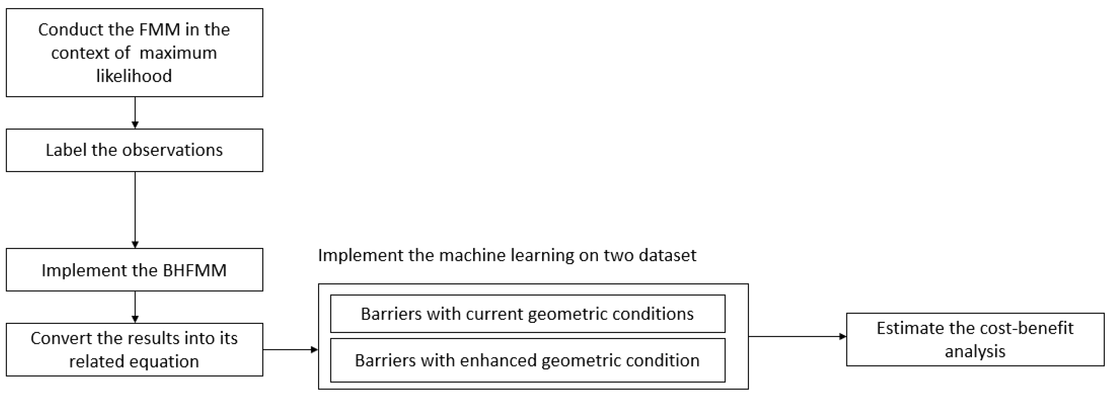
To provide a prioritization process, a monetary evaluation of barrier enhancement was conducted with the help of the machine learning technique. The results of the technique were used to inform policy makers about how much money they would expect to gain after optimizing the underdesigned barriers, and which barriers would be more cost-effective to optimize first. To fulfill these points, several steps were taken in this study, highlighted as follows:
Two barrier types, box beam and W-beam barriers, were aggregated in the dataset on both the state’s highways and the interstate highways. The two barrier types namely: box beam and W-beam, were aggregated in the dataset. It was expected that the data aggregations would result in high heterogeneity. However, to account for the heterogeneity, a finite mixture model (FMM) was used to allocate a cluster to each observation based on their distributions
After a model was trained across all barriers in the state highway and interstate system, the trained model was implemented only on those barriers that were below/above recommended heights
The heights of the barriers were optimized, and the trained model was implemented again to predict costs
The barriers’ optimal heights were selected based on the recommended heights from a literature review
The cost of barrier enhancements were considered in the cost-benefit analysis when barriers were enhanced
All the variables applying the trained model were kept constant, except for shoulder width, barrier height, and their interaction term
After finding predicted EPDOs for years before and after enhancement, the predicted EPDO values were converted to their monetary values so the barrier enhancement cost could be added to the EPDO costs
The barriers were ranked based on their benefits so that WYDOT could first enhance the barriers with higher benefits.
It should be noted that this work is an extension of previous work conducted by the authors [
3]. While the previous work used the Bayesian hierarchical two component model, this method just considers a single component negative binomial. Also, while the previous work could account for zero observations through its first layer, this work, due to its nature, could not optimally account for zero observations so we just consider crash barriers. However, we used another methodology for this paper by accounting for the unseen heterogeneity through a finite mixture, while with a simple negative binomial, the second layer of the previous work, only used a subjective hierarchy assigned to the data. In summary, each method has its strengths and shortcomings as each study took a different approach.
It should be noted that the maximum likelihood method was implemented for FMM instead of the Bayesian technique, due to the shortcomings of the Bayesian technique in estimating clusters, especially labeling the observations. Label switching is a main issue for the Bayesian technique. The problem is due to symmetry in likelihood of the model parameter. Although the problem might be expected to be resolved by removing symmetry by using artificial identifiable constraints, it has been argued that the technique might not be a reliable method for FMM, especially since we used that technique for labeling the observations. The description of the Bayesian hierarchical finite mixture model is detailed in our previous work and the readers are referred to that study [
4]. Thus, maximum likelihood was used for the purpose of the FMM method. The summary of the methodological steps are depicted in
Figure 1.
1.2. Study Contribution
The Bayesian technique has been implemented in various fields, from intrusion to fault detection systems [
5]. On the other hand, the majority of past safety studies in the literature review either focused on the severity [
6] or the frequency of barrier crashes [
7]. However, an inadequate number of studies considered both aspects of barrier crashes: crash severity and frequency. Also, none of those past studies considered geometric characteristics of barriers while performing the optimization. This is partly due to a lack of available information related to traffic barrier characteristics.
Thus, besides considering geometric characteristics of barriers, this study is conducted to consider both the aspects of crash frequency and crash severity by using equivalent property damage only (EPDO) and by aggregating barrier crashes across various barrier IDs. In addition, although several studies and experiments have been conducted to identify recommended dimensions of barrier geometric characteristics, none of those studies have quantified the benefit that could be gained by bringing the barriers to their optimal values based on machine learning techniques.
Other shortcomings of the past studies were the approaches taken to account for heterogeneity. Some studies used FMM to come up with the data models’ distributions. However, those approaches resulted in a loss of information as they divided data into a number of datasets based on various distributions. Another approach is to use the hierarchical technique to account for the heterogeneity in the dataset. However, assignment of data to the hierarchy has been mainly subjective in studies related to traffic safety studies, where there is no clear-cut hierarchy, and the researchers assign data to the hierarchy based on educated or engineering knowledge. Thus, this study is conducted by taking into consideration the aforementioned shortcomings. As not much study has been conducted in the area of optimization in traffic safety the way we did, the readers are referred to the literature review [
3].
This paper is organized as follows: the methodology section outlines the implemented methods, while the data section details the data used in the study. The remaining sections of this study would summarize the results and conclusions.
2. Methodology
This study implemented the Bayesian hierarchical finite mixture model (BHFMM). In this method, after finding the distributions’ parameters of observations, the clusters are assigned to the related observations, and then the resulting dataset is used in a hierarchical technique for analysis and application of machine learning techniques. The following section first outlines the finite mixture model (FMM), and then presents the hierarchical technique, and the model implementation.
2.1. Finite Mixture Model
The FMM is defined as a probabilistic model which can be used to represent the presence of subpopulations within the overall dataset. For instance, in the current dataset, it is believed that there are heterogeneities due to aggregating various datasets such as highway systems, barrier types and seasonality. Although using barrier types or highway systems could account for some heterogeneity in the dataset, just considering those aspects could not account for the full range of heterogeneity. This is especially true as there are several unseen factors that the available predictors as hierarchies could not account for. Not accounting for this heterogeneity issue, due to data subsets having different residuals distribution, biased or erroneous estimates would emerge.
Traditional modeling assumes that all the data comes from the same distribution. Researchers often account for the data heterogeneity by assigning subjective hierarchies. However, no real information is available to determine which observations should be assigned to which distribution. Finite mixture models could be used for those cases to describe the unknown distributions. The finite mixture model with k components could be written as [
8]:
with conditions of:
where
h is a density of
y as dependent variable,
x is a vector of independent variables,
is the probability of component
k, and
is the component-specific parameter for the density function
f.
Due to the response characteristics being non-negative, discrete and posing over dispersion, the negative binomial (NB) model is a good choice for modeling traffic barrier EPDO crashes. Here the NB probability density for a cluster
k is defined based on
and
ψ as:
where the expected value of EPDO,
, is estimated based on
.
is the standard gamma function,
is dispersion parameter.
is mean parameter which is written based on
, the vector of regression coefficients, as:
and the variance of
is written as:
The above equation highlights that for NB, the variance is larger than the mean.
Then NB as a type of generalized linear model is used to explain the relationship between the count response,
y, and various model covariates of
as follows [
9]:
where
g is a link function, and
are regression coefficients. For this study,
follows the negative binomial model with the log link function as
where
were defined earlier. It is worth mentioning that the relationship below exists between the dispersion parameter of
and the overdispersion parameter of α as:
From the above equation, if or the dispersion moves toward zero, the model would become the Poisson model.
2.2. The Bayesian Technique
The Bayesian hierarchical model with j levels is defined with three probabilistic levels [
10]: those include the data model corresponding to observations
, the process model considering the parameters
of the NB where
, and the parameter model setting a probabilistic distribution on the
hyperparameter of
as
.
Here,
is the correlation or dependency across various hierarchies. The parameters of
with normal and gamma distributions, respectively, could be written as follows:
where
are normal distribution parameters of mean and variance, respectively, and
are shape and scale parameters, respectively, of the gamma distribution. Now the discussed hyperparameter
can be written based on:
As the hierarchy in this study was set up for only intercept, and the priors would be set for each predictor coefficient. The term
is set as the gamma distribution as it adjusts dispersion through degree and scale parameters [
11]. Gibbs sampling is implemented for generating
parameters, coefficients and dispersion parameters. For instance, for iteration
r = 1,2,…, there would be:
where
N and
are normal and gamma distributions, respectively. As can be seen from the above equations, as a combination of
NB and
N or Gamma cannot be calculated easily, applications of sampling methods necessitate the identification of those parameters.
Model Syntax in JAGS
In the Bayes method, the posterior probability,
of the coefficients are conditioned and are written as follows:
where
is the prior probability of the model parameters. Another characteristic of the Bayes method compared with maximum likelihood is the Bayes method assumes that the response is drawn from a probability distribution rather than a point estimate.
In the model syntax, the count model should be defined. The NB distribution, compared with the Poisson distribution, requires more parameterizations to have a form making it suitable for modeling sparse datasets. This would be implemented on observation
i with the success parameter p
i and the overdispersion parameter
r, which is greater than 0. The success parameter is written as follows:
where
is a conditional mean which is written as:
A uniform prior was set for parameter r with an upper bound of 50, and a lower bound of zero.
A hierarchical model with only random intercepts is written as follows:
where
is a barrier EPDO count for a certain type of barrier. Subscript
i refers to an individual crash, while subscript
j refers to the hierarchy, which is equal to the number of objective hierarchies (clusters) as 4. For this study,
p is the number of incorporated predictors in the count part. As only random intercepts related to an objective hierarchy were considered, the model coefficients are similar across various barrier types, and only the intercept varies.
A best fit model was identified by considering various predictors as a hierarchy and an objective hierarchy, which was identified through the FMM. For instance, subjective hierarchies which make engineering intuitive sense were considered. Those include considering barrier types or highway systems as hierarchies. Those three models’ performances were compared with an objective hierarchical model assigned by the FMM model.
Identifying a best fit model is important as the finalist model will be used for cost-benefit analysis. The deviance information criterion (DIC) was used as a measure for the models’ performance comparisons [
12]. That method is a generalization of the Akaike information criterion (AIC) in the Bayesian context. The method measures the complexity, and goodness of fit: the complexity is linked to the number of included parameters, while the fit measure is related to the deviance as:
where
is a number of included parameters being used to penalize the model for the number of incorporated parameters. In summary, a best fit model would be identified based on a lower value of DIC.
It is worth mentioning that in the analysis we considered a non-informative prior. For that we consider a wide variance, limited precision, with a mean of zero so the model is able to search for the posterior distribution across a wide range of values. Using a non-precise informative prior would result in erroneous results as the model is limited for sampling from the prior distribution to reach the posterior distribution.
2.3. Cost-Benefit Analysis
Welfare maximization can be defined as the objective of cost-benefit analysis [
13]. The cost-benefit analysis is dependent on the Pareto criterion for checking whether a project increases welfare or not. This idea is based on the ideal welfare scenario where a policy improvement makes some people better off while nobody would experience a loss. However, in reality, projects make some people better off, while others would be worse off. As a result, economists pledge to a less demanding state: a project satisfies the criterion when those who benefit from a project, compensate those who lose from it [
13].
The same concept was implemented in this study. If overall, the total benefit is to be positive, optimizing would be cost-effective. Also, a higher priority is given to a higher total benefit based on the analysis. The benefit over a 10-year period based on equivalent property damage only (EPDO) could be written as:
And the total benefit is calculated as:
The value of $34,612 is the cost of PDO in Wyoming based on the state criteria: after coming up with EPDO, the value would be converted into costs. It should be noted that the cost of barrier enhancements would be added just for the first year in Equation (19).
In Equation (19), costs at year i would be estimated based on the interpolated traffic in that year. Based on the last 10-year historical traffic data, traffic in the state highway system was almost constant. However, the interstate system traffic increased by a rate of 4% in 10 years or for every year. The costs of the barriers’ resets would be executed only for the first year.
Based on WYDOT’s recommended values, EPDO is written as:
Now after converting every crash severity level to PDO in Equation (21), with the same sequence of variables, it follows that [
3]:
where for instance, a fatal crash is equivalent to 277 EPDO crashes, from Equations (21) and (22).
In summary, the methodological optimization steps taken in this study are summarized as follows:
Dataset preparation: Filter the data to include barriers experiencing crashes on state highway and interstate systems in Wyoming
Barrier types: Filter data to include only box beam and W-beam barriers since other barriers only account for a small proportion of the dataset
Data aggregation: Aggregate the crash data across traffic barriers and traffic datasets, based on mileposts and roadway IDs. Also consider the relation of various demographic and environmental factors to crashes. For instance, if barrier ID 1234 experienced 10 crashes, based on EPDO, the average of various explanatory variables such as driver and environmental characteristics would be aggregated over that barrier ID
Hierarchy setting: Identify a best choice of variable for the model hierarchy, based on the lowest DIC
Convert the best fit model in step 4 into an equation
Data preparation: train the model on the dataset including all barriers that experienced at least one crash
Implement the trained model on a test dataset with barriers’ current heights: based on current barriers’ geometric characteristics. Also, for each year, consider an increase in traffic for the interstate system only
Implement the trained model on the test dataset with the barriers’ enhanced heights: based on enhanced barriers’ geometric characteristics. Also, include an increase in traffic for the interstate system only and consider the reset costs
Calculate benefit based on Equation (20)
Report the total savings
Sort barriers based on the highest benefits and report it
2.4. Optimum Traffic Barrier Heights
In the optimization process, the barriers would be optimized to an optimal value based on the recommended range found in the literature review. Different values based on various experiments were highlighted for both box beam and W-beam barriers ranging from 27 to 31 inches [
14,
15]. To be consistent, a cutting value of 27 inches was chosen as a value for all the barriers for the optimization process.
3. Data
Three sources of datasets were aggregated to create a final dataset. The data sources include traffic, crash, and barrier geometric characteristics. The Wyoming Department of Transportation (WYDOT) provided the crash and traffic datasets between 2007 and 2017. The traffic dataset includes predictors such as average annual daily traffic (AADT) and average annual truck traffic (ADTT).
The second dataset was the barrier geometric dataset including different roadway, and barrier geometric characteristics such as types, length, offset, and height of barriers. This dataset also includes various roadside geometric characteristics such as shoulder width. In addition, the data incorporated the starting and ending mileposts of traffic barriers on the roadways, and the roadway ID along with its direction. In addition, only crashes involving hitting a barrier as their first harmful event were included in the dataset. The crash dataset was aggregated across various barriers based on the milepost, direction of travel, and highway system.
Table 1 presents summary statistics of those predictors that were found to be important in the statistical analysis. A few points are worth mentioning from
Table 1. Some barriers experienced more than a single crash. For those scenarios, the average of various drivers’ characteristics, and weather or road conditions were used as explanatory variables across those barriers. For instance, if two drivers with two residencies, Wyoming residence as 0 and non-Wyoming residence as 1, hit a barrier ID of 1234, the average of those crashes as 0.5 would be set for residency variable for barrier ID 1234.
The concrete barriers accounted for a total of 2% of all barriers and the majority of those barriers in the dataset were higher than 42 inches. As a higher concrete barrier could not result in underride crashes, those barriers were excluded from the optimization process. A binary category was assigned to shoulder widths. A shoulder width less than or equal to 1.5 feet was categorized as 0 while other values were considered as 1. It should be noted that clusters I to IV are based on the FMM model.
4. Results
This section is presented in three subsections. An identification of a best fit model across three considered models is discussed in the first section, while the finalist model results, and its brief discussion are presented in the second section. The mathematical optimization process includes the implemented method being used to convert the results into an equation for use as a machine learning technique. The last section, optimization results, presents the optimization results of the cost-benefit analysis of the barriers with the highest benefits.
4.1. Best Fit Model
Three models were considered in this study based on various intuitive variables as hierarchies and the objective hierarchy assigned by the FMM. Those models were compared in terms of goodness of fit based on the DIC. The assigned objective hierarchies resulted in a lower DIC of 11,057, compared with the state highway system as a hierarchy with DIC = 11,063, and barrier types as a hierarchy with DIC of 11,060. Thus, due to lowest DIC value, an objective hierarchy was used for the analysis. The sum of the predicted EPDO and real EPDO along with their variances are presented in
Table 2. The results from using subjective hierarchies are not presented in
Table 2 to conserve space.
Although the range between the sum of the predicted and real EPDO is not too wide, the variance difference of these two variables are rather wide. This is likely due to the randomness of crashes. For instance, the maximum of the predicted EPDO is 1733. This high value is related to the fact that this observation has the worst criteria based on the statistical results: for instance, the majority of drivers hitting this barrier were male, occurring on the interstate system with a long barrier length.
Since the objective of this study is not just about conducting statistical analysis, but rather the application of machine learning techniques, this study does not detail the analytical results. For instance, the results highlight that being unrestrained, being female drivers, being a non-Wyoming resident, and driving in adverse weather conditions reduce the likelihood of the number of the EPDO crashes. Although for some predictors some minor uncertainty about the significance of the predictors is observed, the important predictors of interaction of shoulder width and barrier heights were found to be significant. It should be noted that barrier types, shoulder width, AADT, and barrier length were considered especially to account for exposure. Alpha [
1] to alpha [
4] are the clusters assigned to the model hierarchy while B0 is an intercept. It should be noted the Sum of real EPDO is 28,945, while the sum of predicted EPDO is 17,084. On the other hand, variance of real EPDO is 30,942, and the variance of predicted EPDO is 1355. Again the findings’ comparison across models, more consistent results for predictions values, are in line with the previous study [
3].
4.2. Mathematical Optimization Process
The BHFMM model was identified as a best fit model. Thus, the results of the modeling were converted into an equation and used for a machine learning technique. The NB process is simple and straightforward: it consists of multiplication of the estimated coefficients with the related variables and then exponentiation of the sum of the above and rounding to the nearest value to calculate the expected number of crashes. The estimation process would slightly vary by considering various hierarchy intercept for each observation.
A function was made to increase the traffic by a value of 0.04/10 for each year if that barrier belongs to an interstate system, while keeping the traffic the same if a barrier is on the state highway system. Thus, traffic was calculated for every year during the 10-year period.
Another function was made to implement the interpolated traffic into an equation for barriers with and without enhancement. Barriers’ predicted EPDOs without enhancement were calculated by using the interpolated traffic and original heights of barriers. On the other hand, the same process was used for barriers after enhancement, with the difference being that the barrier heights were changed to a value of 27 inches. As the values are based on EPDOs, those were multiplied by the expected cost of a single PDO, which is $34,612. It should be noted that after converting crashes into costs, the cost of barrier enhancement was also incorporated in the calculations.
4.3. Optimization Results
As discussed in the above section, the applied mathematical process resulted in the identification of benefits that would be gained by optimizing barrier heights.
Table 3 presents the barriers with the highest benefits based on the machine learning technique. In general, lower variance is observed by conducting the machine learning technique compared with real EPDO. That is expected as the machine learning, algorithm, follow specific rule while crashes are random. The results are in line with the literature review [
3].
Based on the identified results in
Table 3, and a discussion based on the mathematical optimization process, when the shoulder width is less than or equal to 1.5 feet, and the category is 0, an increase in the barrier height would result in a benefit in terms of crash savings as the shoulder width terms and interaction terms would be zero, and would not come into play a role in estimating the benefit.
On the other hand, when the shoulder width is greater than 1.5, coded as 1, the benefit would be obtained mainly from barriers with extremely low height. For instance, consider a scenario where the barrier height is less than a foot. Based on the results in
Table 2, the multiplication of the interaction term by the barrier height, +0.903 × barrier height, would not surpass the multiplication of the coefficient of barrier height with its height, −0.926 × barrier height.
Again, it should be noted that barriers from the test dataset included only those barriers outside the recommended barriers’ heights, including above 36” and below 27”.
Table 3 presents the topmost cost-effective barriers identified based on the machine learning technique. As can be seen from
Table 3, the most cost-effective barriers are those with the lowest heights.
From
Table 3, mostly the state highway barriers were highlighted as barriers that are most cost effective. This is mostly due to very low barrier heights in the highway system. The barriers were included in
Table 3 up to the first interstate barrier. As shown at the bottom of
Table 3, if all barriers not meeting current standards are to be fixed, the total cost will be
$4,632,372 while the overall benefit will only be
$3,418,717.
5. Conclusions
In this study, cost-benefit analysis, with the help of machine learning techniques, was utilized to estimate the benefit of upgrading the heights of Wyoming road barriers to their standards. Due to the randomness of crashes and the low volume of traffic in the state, a severe sparsity in the dataset could be observed for the frequency of barriers’ crashes. The high sparsity was accompanied by severe data heterogeneity resulting from integration of various barrier types and highway systems. It is hypothesized that due to high heterogeneity and sparsity of the dataset, ignoring those shortcomings would result in erroneous and biased results. Thus, to address the issue of sparsity, the negative binomial distribution was implemented. Also, to account for the data heterogeneity, various parameters such as state highway systems, barrier types and objective clustering through FMM were considered as a hierarchy of the model. Not accounting for heterogeneity or sparsity of the data could result in biased or erroneous results. The modeling methodology was conducted in the context of the Bayesian method.
With regard to objective clustering, the FMM was conducted and the optimum number of clusters was identified. The FMM was conducted in the context of maximum likelihood due to the label switching issue of the method in the Bayesian context. The identified clusters were assigned to each observation. In the next step a Bayesian hierarchical model with the FMM hierarchy was compared with subjective intuitive clustering, e.g., the state highway systems and barrier types. Models were compared and the model with a best assigned hierarchy was chosen. Deviance information criterion (DIC) was used for model selection.
Predicted EPDO crashes for each year were based on interpolated traffic. The barriers’ heights were changed to their optimum values and the machine learning technique was implemented again. The predicted cost for barriers with and without enhancement were summarized and the barrier optimization costs were considered. The difference in crash costs before and after height adjustments was calculated as a total benefit.
In summary, the results indicated that after investing money to bring under-design barriers to their optimum heights, WYDOT would not only recover the invested money in 10 years but they would also expect to save more than $4 million dollars in crash savings through the optimization process of the barriers. Although the analysis highlights the interaction terms between both shoulder width and barrier heights, the shoulder width was left constant, and only barrier heights were optimized. If the constraint was set free, more benefits would have been gained by optimizing both barrier heights and shoulder width.
This study is one of the first studies that quantifies the monetary benefit of optimizing the heights of traffic barriers. More studies are needed to quantify other aspects of traffic enhancement through machine learning techniques. The WYDOT could utilize the ranking list developed in this analysis to allocate funding to upgrade all traffic barriers in the state. The upgrade might take a few years considering the total amount of needed funding, and limited safety funds statewide.


