Lumáwig: An Efficient Algorithm for Dimension Zero Bottleneck Distance Computation in Topological Data Analysis

Abstract

Stability of persistence diagrams under slight perturbations is a key characteristic behind the validity and growing popularity of topological data analysis in exploring real-world data. Central to this stability is the use of Bottleneck distance which entails matching points between diagrams. Instances of use of this metric in practical studies have, however, been few and sparingly far between because of the computational obstruction, especially in dimension zero where the computational cost explodes with the growth of data size. We present a novel efficient algorithm to compute dimension zero bottleneck distance between two persistent diagrams of a specific kind which runs significantly faster and provides significantly sharper approximates with respect to the output of the original algorithm than any other available algorithm. We bypass the overwhelming matching problem in previous implementations of the bottleneck distance, and prove that the zero dimensional bottleneck distance can be recovered from a very small number of matching cases. Partly in keeping with nomenclature traditions in this area of TDA, we name this algorithm Lumáwig as a nod to a deity in the northern Philippines, where the algorithm was developed. We show that Lumáwig generally enjoys linear complexity as shown by empirical tests. We also present an application that leverages dimension zero persistence diagrams and the bottleneck distance to produce features for classification tasks.

1. Introduction

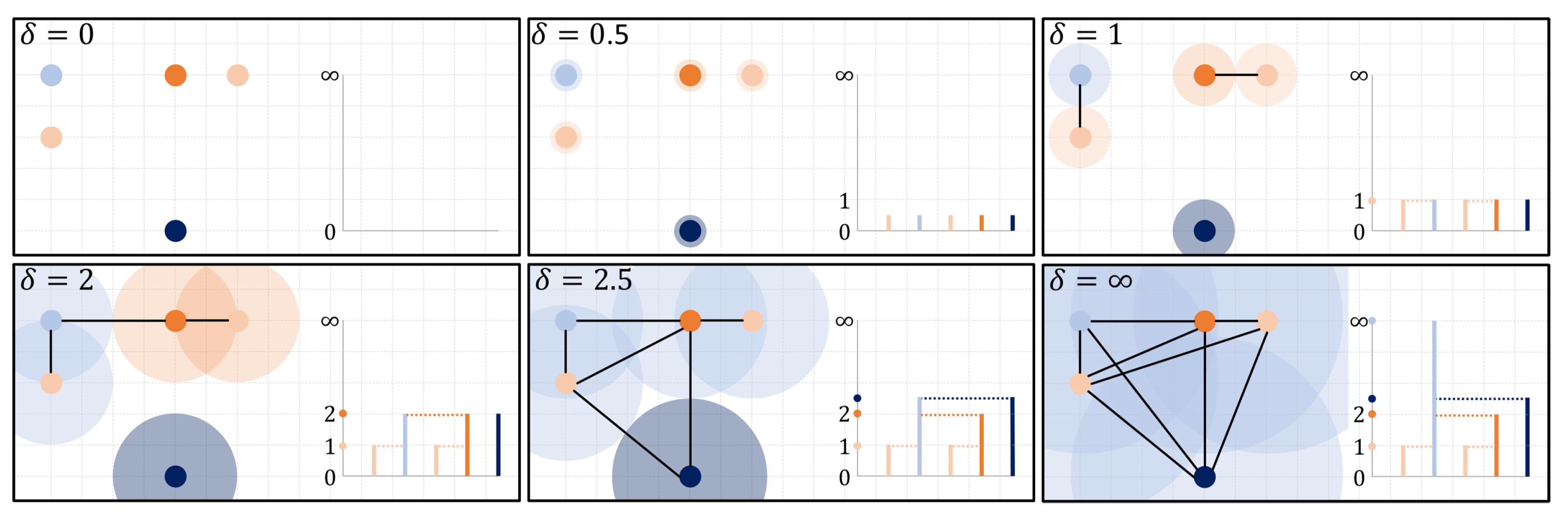
Topological data analysis (TDA) has gathered significant interest from a wide range of researchers because of its novel approach and use of classical tools from algebraic topology for extracting descriptive features from data. Succinctly, topological data analysis captures and records the persistence [1,2] of algebraically computable topological signatures, and regards it as a measure of significance for different features embedded in the structure of data. For the zero dimensional case, these signatures correspond to clusters within data that merge based on a filtration of the data points. One of the most common filtration used in practice is the Rips filtration where pairs of points are considered merged at a given filtration slice $\delta$ when the points are at most $\delta$ apart. Hence, as opposed to other filtrations that require additional parameter choices, the Rips filtration only depends on intrinsic distances between data points and reveals the underlying multi-scale connectivity information about natural clusters existing within data. The Rips filtration produces summaries of topological signatures all beginning at the start of the filtration, capturing cluster merging dynamics akin to that observed by hierarchical clustering methods (see Figure 1). This is the setting we will be working on.

Meriting the growing popularity for this approach, and central to its relevance and viability in interrogating real-world data, is its stability under slight perturbations—small discrepancies between measurements within data lead to small differences in the recorded persistence of features. This cornerstone stability result [3] relies on classic bottleneck matchings to evaluate, measure, and bound changes between two records of feature persistence. These records, called persistence diagrams, are a collection of points in the extended plane where the coordinates represent the birth and death times of the recorded features. In these diagrams, points that have multiplicity capture distinct features with the same birth-death profile, and points with infinite persistence capture perpetual features. For diagrams induced by the Rips filtration, the sole constant perpetual feature appears in dimension 0, capturing the eventual single cluster that merges all components (see Figure 1).

Given two persistence diagrams X and Y, the bottleneck distance between them is defined as

$$d_B(X,Y)=\underset{\varphi }{inf}\underset{x\in X}{sup}\left|\right|x-{\varphi \left(x\right)\left|\right|}_{\infty }$$

where the infimum is taken over all bijections $\varphi :X\bigsqcup \Delta \to Y\bigsqcup \Delta$ and $\Delta$ is the diagonal. In general terms, the bottleneck distance measures the cost to transform one diagram to another. The first, and for a long time the only, publicly available implementation of the bottleneck distance for persistence diagrams is in the library Dionysus, released in 2010, by Morozov [4]. This implementation uses a variant of the Hungarian algorithm [5] for the assignment problem.

Understandably, because of the overwhelming matching step in the computation, this first implementation of the bottleneck distance between two persistence diagrams was considerably slow by practical standards. Consequently, while the theoretical side of topological data analysis has made extensive use of the bottleneck distance for advancing the theory [6,7,8], first computational uses have been few and sparingly far between. Some notable examples include applications to classification of hepatic lesions  [9], and analysis of time-series data [10] and simulated hippocampal networks [11]. Most applications of TDA, instead, tap into persistence-based topological features via another class of objects, called persistence landscapes [12], that record the persistence of features as a function, thus affording access to desirable properties of the underlying function space. A major motivation for this detour to landscapes is the ability to generate topological summaries that are compatible with classical tools in statistics, and even machine learning.

In 2017, Morozov et al. [13] provided an improved implementation of the bottleneck distance in the library Hera by exploiting geometry. Their approach follows closely the work of Efrat et al. [14]. For the sets $X_0$ and $Y_0$ of orthogonal projections on the diagonal $\Delta$ of points respectively from X and Y, and the sets $U=X\cup Y_0$ and $V=X_0\cup Y$, they consider the weighted complete bipartite graph $G=(U\bigsqcup V,U\times V,w)$ where $w:U\times V\to {\mathbb{R}}_{\ge 0}$ is given by

$$w(u,v)=\left\{\begin{array}{cc}\left|\right|u-{v\left|\right|}_{\infty }\hfill & \mathrm{if} u\in X \mathrm{or} v\in Y\hfill \\ 0\hfill & \mathrm{otherwise}.\hfill \end{array}\right.$$

With this, the bottleneck computation problem can be recast in the following manner: if $G\left[r\right]$ is the subgraph of G with all edges e of weight $w\left(e\right)\le r$, then the bottleneck distance of G is the minimal value r such that $G\left[r\right]$ contains a perfect matching. Hence the bottleneck distance can be recovered by combining a binary search on the edge weights of G with a test for a perfect matching. For the matching step, they augment the Hopcroft-Karp algorithm [15] by appealing to a near-neighbor data structure (a k-d tree) to search for the best candidate pair for a query point, pruning from the search the subtrees (and hence all other candidates within them) whose enclosing box is further away from the query than the current best candidate. This circumvents the overwhelming matching problem by significantly shrinking down the combination pool to retrieve the best matching. To approximate complexity, they fit curves of the form $c{n}^{\alpha }$ and found a best fit with $\alpha =1.4$. This translates to speed-up from Dionysus already by a factor of 400 on diagrams with 2800 points, and opened opportunities for several works that examine larger [16] or more complex [17,18] data sets.

We take inspiration from this idea of exploiting the geometry of persistence diagrams to extract computational speed-up. By considering dimension 0 persistence diagrams induced from the Rips filtration, we can approach the problem via a different framework, birthing a new efficient algorithm for computing the bottleneck distance. The key idea is to begin with a specific initial bijection that one can methodically modify to optimize the norm between matched points. This process allows us to identify all possible instances where the bottleneck matching is achieved, and the exact value for the bottleneck distance, significantly bypassing the overwhelming matching step in previous implementations. We remark that while this strategy only works for persistence diagrams of a specific kind—those whose detected signatures all begin at the same time—this class is in no way less significant than diagrams induced from other filtrations. Moreover, in addition to diagrams induced from the above setting, this class also includes diagrams obtained from the output of any hierarchical clustering algorithm applied to point cloud data. Hence, the computational speed-up for the bottleneck distance we obtain benefits the comparison of these diagrams as well. Furthermore, we note that there are other metrics used in the literature to compare persistence diagrams, and we make no preference claim in favor of the bottleneck distance. In fact, it is a good question to ask whether the above strategy can be followed to generate computational speed-up for these metrics as well (We credit Katharine Turner for raising this question first in relation to the Wasserstein distance.).

We name this algorithm Lumáwig. Lumáwig is significantly faster than the state-of-the-art and provides significantly sharper approximates with respect to the output of the original algorithm than any other available algorithm. We benchmark Lumáwig against all available algorithms in terms of running time and accuracy.

Our motivation for this work is to clear the computational obstruction in the use of bottleneck distance in applications. In the Filipino language, Lumáwig also means to extend, broaden, or expand. Our hope is that this contribution will serve as a catalyst in the further development of the theory that leverages persistence diagrams and the bottleneck distance similar to what has been achieved for persistence landscapes, and will usher in a new era of integrating TDA into the science of big data. As a proof of concept, we use Lumáwig to generate features for the classification of digit images from the MNIST data set.

2. Bypassing Matchings

We propose to bypass the overwhelming matching problem in the computation of 0-dimensional bottleneck distance by showing that the value produced by the bottleneck distance formula can be recovered by considering only a few cases. We will show that these cases naturally come up in the process of minimizing the output of the norm.

We first note that for most practical applications to data analysis of 0-dimensional persistence diagrams, where all components are assumed to be born at the beginning of the filtration for persistent homology, all non-trivial points lie in the vertical axis (or equivalently for persistence barcodes, all bars begin at time $t=0$). Hence, in this case, if ${\delta }_x$, and ${\delta }_{\varphi \left(x\right)}$ are the death times respectively for x and its matched point $\varphi \left(x\right)$, we have that

$$\left|\right|x-{\varphi \left(x\right)\left|\right|}_{\infty }=\left\{\begin{array}{cc}max({\delta }_x,{\delta }_{\varphi \left(x\right)})/2\hfill & \mathrm{if}\varphi \left(x\right)\in \Delta \hfill \\ |{\delta }_x-{\delta }_{\varphi \left(x\right)}|\hfill & \mathrm{otherwise}.\hfill \end{array}\right.$$

(1)

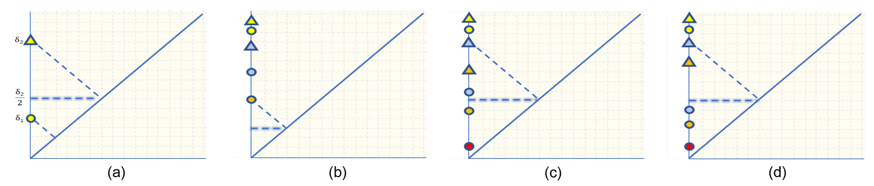
This suggests that while it is natural to do a point-to-point matching between diagrams, there are cases when we are better off matching a point to the diagonal. For a point $x\in X$ and $\varphi \left(x\right)\in Y$, this happens precisely when

$$max({\delta }_x,{\delta }_{\varphi \left(x\right)})>2min({\delta }_{\varphi \left(x\right)},{\delta }_x).$$

(2)

Figure 2a illustrates this point. Therefore, unless (2) is satisfied, it is our priority to match a non-trivial point in a diagram X with a non-trivial point in another diagram. This supports the interpretation that the bottleneck distance is the cost of transforming one diagram to another.

We are now ready to present our algorithm for computing 0-dimensional bottleneck distance between two persistence diagrams. We first induce and ordering of the death times in both diagrams and define a bijection that we can methodically modify to optimize the norm between matched points and recover the desired matching that achieves the bottleneck distance. The proof of Lemma 1 provides the basic argument that allows us to bypass the overwhelming matching problem. Lemma 2 proceeds in the same manner and identifies all other possible instances where the bottleneck matching is achieved, and the exact bottleneck distance in each case.

Let X and Y be two 0-dimensional persistence diagrams whose death time entries are arranged from largest to smallest. Equivalently, X and Y can be thought of as persistence barcodes whose bars are arranged from longest to shortest. Without loss of generality, assume that X has at most as many points as Y has. We remark that this pre-processing is equivalent to considering the bijection $\varphi$ that matches points between X and Y according to the relative ranking of death times from largest to smallest, and where unmatched points in Y are matched to the diagonal. Let $N=length\left(X\right)$ and define

$$Z={\left[z_i\right]}_1^{length\left(Y\right)}\mathrm{where}{z}_i=\left\{\begin{array}{cc}|x_i-y_i|\hfill & \mathrm{if}i\le N\hfill \\ y_i/2\hfill & \mathrm{otherwise}\hfill \end{array}\right.$$

and $l=arg\; max\left(Z\right)$.

Lemma 1.

Let X, Y, Z, N and ϕ be defined as above. If $N<length\left(Y\right)$ and $max\left(Z\right)\le y_{N+1}/2$, then

$$d_B(X,Y)=y_{N+1}/2$$

where $y_{N+1}$ is the largest death time of a point in Y matched to the diagonal.

Proof. 

For the bijection $\varphi$ corresponding to the pre-processing described above, it follows that

$$\underset{x\in X}{max}\left|\right|x-{\varphi \left(x\right)\left|\right|}_{\infty }=y_{N+1}/2.$$

Figure 2b illustrates this case where the point matched to the diagonal maximizes the norm. To see why $\varphi$ achieves the infimum over all bijections between X and Y, note that any other bijection $\psi$ produces a death time for a point in Y matched to the diagonal that is at least as large as $y_{N+1}/2$. Therefore ${max}_{x\in X}\left|\right|x-{\varphi \left(x\right)\left|\right|}_{\infty }\le {max}_{x\in X}\left|\right|x-{\psi \left(x\right)\left|\right|}_{\infty }$. □

Lemma 2.

Let X, Y, Z, N, l and ϕ be defined as above, and let ζ be the second largest entry of Z.

1. 

If $max\left(Z\right)\le max(x_l,y_l)/2$, then $d_B(X,Y)=max\left(Z\right).$

2. 

If $\zeta <max(x_l,y_l)/2<max\left(Z\right)$, then $d_B(X,Y)=max(x_l,y_l)/2.$

3. 

If $\zeta \ge max(x_l,y_l)/2$ and $m\ge l$ for every m such that $z_m\ge max(x_l,y_l)/2$, then $d_B(X,Y)=max(x_l,y_l)/2.$

4. 

If $\zeta \ge max(x_l,y_l)/2$ and there exists $m<l$ such that $z_m\ge max(x_l,y_l)/2$, then there exists a bijection τ between X and Y such that one of the three preceding cases holds and where

$$max\left|\right|x-{\tau \left(x\right)\left|\right|}_{\infty }<max\left|\right|x-{\varphi \left(x\right)\left|\right|}_{\infty }.$$

Proof. 

1.

It follows from our remark immediately after (1) that

$$max\left|\right|x-{\varphi \left(x\right)\left|\right|}_{\infty }=max\left(Z\right)\le max(x_l,y_l)/2=max\left|\right|x-{\varphi }^{\prime }\left(x\right){\left|\right|}_{\infty }$$

where ${\varphi }^{\prime }$ is the bijection that matches both $x_l$ and $y_l$ to the diagonal, and coincides with $\varphi$ otherwise. Figure 2c illustrates this comparison between the two matchings. For any other bijection $\psi$, if $x^{\prime }\in X$ such that $|x^{\prime }-\psi \left(x^{\prime }\right)|$ is maximum among all non-trivial matchings, either $max\left(Z\right)\le |x^{\prime }-\psi \left(x^{\prime }\right)|$, or $max(x_l,y_l)\le max(x^{\prime },\psi \left(x^{\prime }\right))$. If $N<length\left(Y\right)$, then a similar argument as that in Lemma 1 holds. The conclusion now follows.

2.

In this case, the same bijection ${\varphi }^{\prime }$ in the previous case yields

$$max\left|\right|x-{\varphi }^{\prime }{\left(x\right)\left|\right|}_{\infty }=max(x_l,y_l)/2<max\left(Z\right)=max\left|\right|x-\varphi \left(x\right){\left|\right|}_{\infty }.$$

The same argument in the previous case holds for any other bijection $\psi$. Hence, the inequality above implies the conclusion.

3.

For the bijection ${\varphi }^{″}$ that sends $x_m$ and $y_m$ to the diagonal for all such m, and coincides with $\varphi$ otherwise (see Figure 2d), we have that

$$max\left|\right|x-{\varphi }^{″}{\left(x\right)\left|\right|}_{\infty }=max(x_l,y_l)/2<max\left(Z\right)=max\left|\right|x-\varphi \left(x\right){\left|\right|}_{\infty }.$$

Again, since the same argument in the first case holds for any other bijection $\psi$, the previous inequality implies the conclusion.

4.

Define the bijection $\tau$ that sends $x_j$ and $y_j$ to the diagonal for all $j\ge l$, and coincides with $\varphi$ otherwise. Then we have that

$$max\left|\right|x-{\tau \left(x\right)\left|\right|}_{\infty }<max\left(Z\right)=max\left|\right|x-{\varphi \left(x\right)\left|\right|}_{\infty },$$

Moreover, note that $max\left|\right|x-{\tau \left(x\right)\left|\right|}_{\infty }$ depends only on $\left|\right|x-{\tau \left(x\right)\left|\right|}_{\infty }$ for non-trivially matched x and $\tau \left(x\right)$. Therefore, we can consider only the subsets $X^{\prime }$ and $Y^{\prime }$ respectively of X and Y whose points are non-trivially matched by $\tau$. In this case, $length\left(X^{\prime }\right)=length\left(Y^{\prime }\right)$ and one of the three previous cases above holds.

The proof is now complete. □

The two Lemmas above provide the theoretical basis for the bypass approach of the Lumáwig algorithm. Together, they take advantage of the specific form of dimension zero persistence diagrams being considered, and the methodical approach to optimize norms induced by a specific matching. The complete pseudo code is given in Algorithm 1 below.

Algorithm 1Lumáwig algorithm for computing 0-dimensional bottleneck distance between two persistence diagrams

1: Input: Two dimension zero persistence diagrams X and Y such that $X\ne Y$ and where X has fewer than or as many points as Y.

2: Output: The bottleneck distance between X and Y.

3: Initialization $d\leftarrow 0$, $X\leftarrow$ death times of points from X sorted from largest to smallest, $Y\leftarrow$ death times of points from Y sorted from largest to smallest, $N=length\left(X\right)$, $Z\leftarrow$ vector $[z_i:=|x_i-y_i|{]}_1^N$, $l=arg\; max\left(Z\right)$, $d_{temp}=max\left(Z\right)$

4: if $length\left(X\right)\ne length\left(Y\right)$ and $d_{temp}<y_{N+1}/2$ then

5:     $d=\left(y_{N+1}\right)/2$;

6: else

7:     while $length\left(Z\right)>1$ do

8:         if $\mathrm{Second}\mathrm{largest}\mathrm{entry}\mathrm{of}Z<max(x_l,y_l)/2<d_{temp}$ then

9:            $d=max(x_l,y_l)/2$

10:            $break$

11:         else if $\mathrm{Second}\mathrm{largest}\mathrm{entry}\mathrm{of}Z\ge max(x_l,y_l)/2$ then

12:            if For every m for which $z_m\ge max(x_l,y_l)/2$, $m\ge l$ then

13:                $d=max(x_l,y_l)/2$

14:                $break$

15:            else

16:                Trim off all $z_m,x_m,y_m$ for $m\ge l$; update l and $d_{temp}$

17:                if $length\left(Z\right)=1$ then

18:                    $d=min(d_{temp},max(x_l,y_l)/2)$

19:                    $break$

20:                end if

21:            end if

22:         else

23:            $d=d_{temp}$

24:            $break$

25:         end if

26:     end while

27: end if

3. Benchmarking

We perform two stages of benchmarking against other publicly available implementations of the bottleneck distance. The first stage is in terms of computational running time and relative difference with respect to the original algorithm implemented in the Dionysus library included in the R package TDA [19]. This stage involves persistence diagrams with as many as 900 points and highlights the computational obstructions with current implementations of the bottleneck distance.

The second stage is also done in terms of running time, but the relative difference is with respect to the R implementation of Lumáwig. Only the faster implementations are considered in this stage as it involves persistence diagrams with as many as 30,000 points.

3.1. Benchmarking against All Available Algorithms

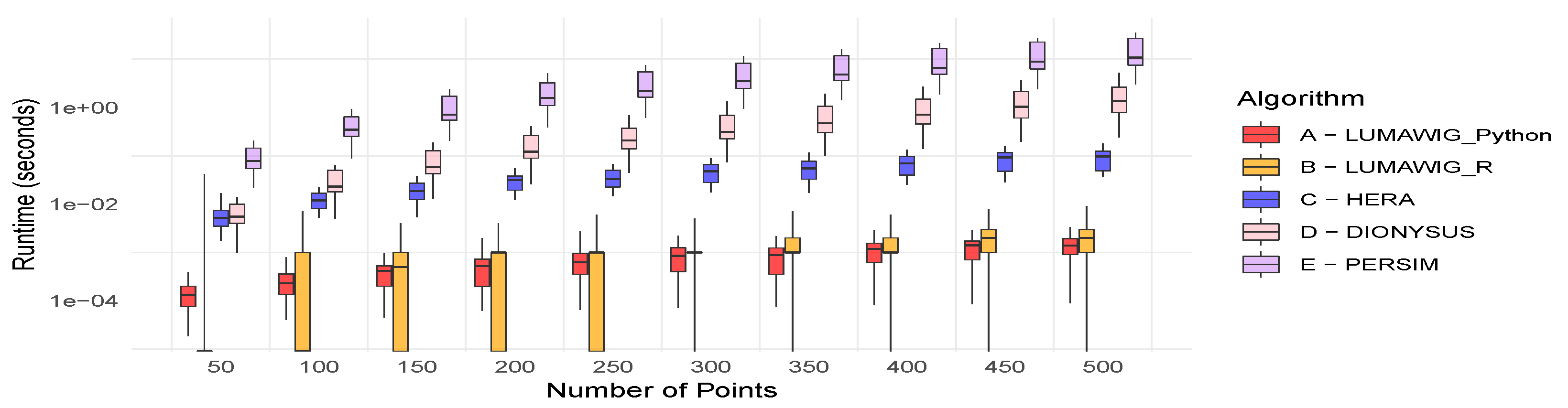
Figure 3 shows the running time (in seconds) of four algorithms for computing the bottleneck distance between two persistence diagrams: the Dionysus implementation (in R), the current state-of-the-art Hera (implemented in C++ and wrapped in Python), a new implementation Persim (Python) [20], and Lumáwig, implemented both in R and Python. The benchmarking is done by first simulating 100 0-dimensional persistence diagrams with 50 points. Each dimension zero persistence diagram is simulated using a set of positive numbers as death times uniformly chosen from a range twice as wide as the number of points. We pair each diagram with another simulated diagram not necessarily with the same number of points (as much as $80\%$ more or less points), then compute the bottleneck distance (up to 10 decimal places) between the pair using the bottleneck implementations above. The running time of each algorithm is recorded, and the distribution summary of 100 run times for each algorithm is plotted out as a boxplot. For Hera, we follow the experimental setup from [13] and set $\delta =0.01$. We repeat this process while increasing the number of points in the base persistence diagram by 50 until we reach 500 points for each base persistence diagram.

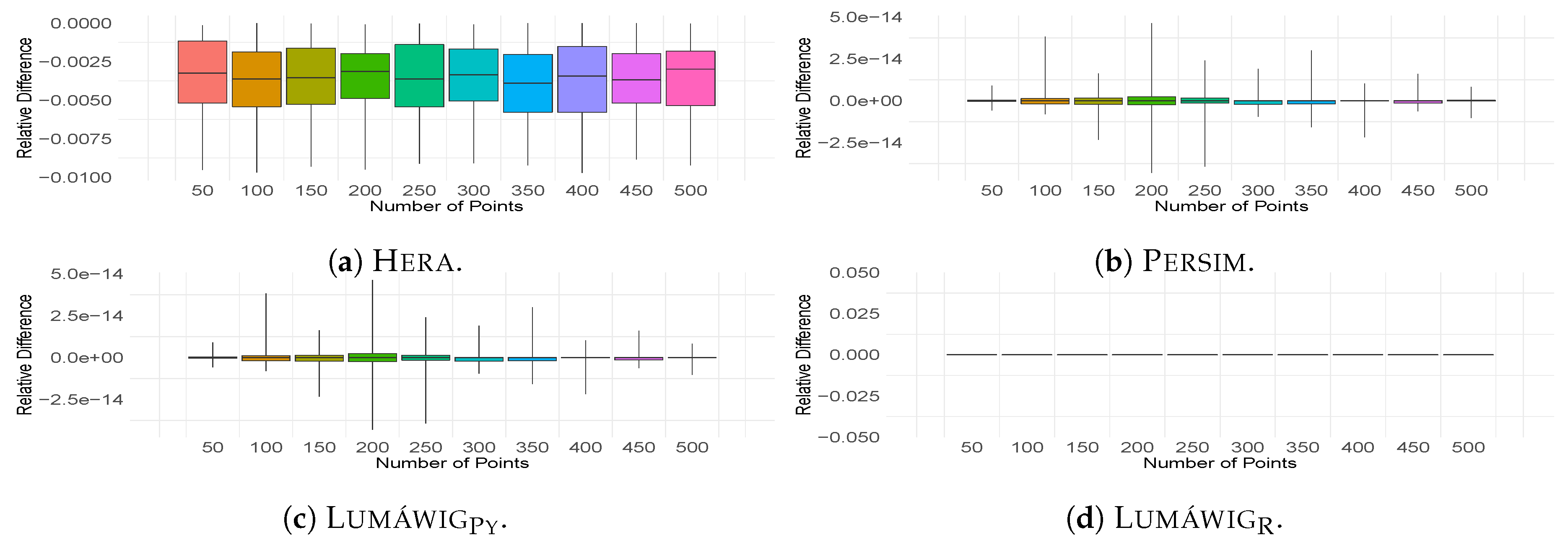
We also compare the computed bottleneck distance against the output of Dionysus. Relative differences of the outputs of three other implementations from Dionysus are computed for all 100 pairs of persistence diagrams. From these bottleneck computations, descriptive summaries are obtained and plotted as boxplots in Figure 4. Is it worth noting that Hera consistently overestimates the zero dimensional bottleneck distance relative to Dionysus as seen in Figure 4a. Another important observation is that the output of Lumáwig_Py recovers that of Persim at a much less computational running time. Finally, we highlight that Lumáwig${}_{\mathsf{R}}$ recovers the exact output values of the original implementation in Dionysus.

We remark here that while this stage of benchmarking is indeed confined within extremely small data sets, this situation in fact represents what is currently accessible to most researchers, and highlights the clear computational obstruction in the use of persistence diagrams and bottleneck distance in applications with currently available algorithms.

3.2. Benchmarking Lumáwig on Larger Data Sets

We perform a second stage of benchmarking against the current state-of-the-art implementation of the bottleneck distance in Hera. We again simulate 100 0-dimensional persistence diagrams and pair each diagram with another simulated diagram not necessarily with the same number of points. Similar descriptive measures as in the earlier stage are considered from the 100 pairs of diagrams with increasing number of points from 1000 to 30,000. The choice of benchmarking bottleneck computation to at most 30,000 points was to draw comparison with that of Hera in [13]. One difference in our benchmarking is that the number of points in the two diagrams we are comparing need not be equal.

Figure 5 shows the running time distribution of 100 dimension zero bottleneck distance computations over increasing diagram sizes. Please note that the vertical axis is displayed in logarithmic scale. Only five boxplots for the running time of the original algorithm implemented in Dionysus are superimposed to provide reference for the state-of-the-art Hera and our two implementations of Lumáwig. A quick inspection reveals that both implementations of Lumáwig are consistently several orders of magnitude faster than the current state-of-the-art Hera. The use of the same pairs of simulated persistence diagrams for bottleneck computations across implementations allowed for paired tests of significant difference in running time relative to Hera. These significant values, computed at $\alpha =0.95$ level of confidence, appear in

Table 1. Summary of significant decrease (at confidence level $\alpha =0.95$) in running time (in seconds) for paired tests versus Hera. Column labels are in thousands of points.

	1	2	3	4	5	6	7	8	9	10
LumáwigR	0.230	0.651	1.203	1.971	2.744	3.957	5.003	6.813	8.348	9.983
LumáwigPy	0.231	0.659	1.221	2.004	2.797	4.037	5.107	6.928	8.498	10.181
	11	12	13	14	15	16	17	18	19	20
LumáwigR	11.029	12.227	14.985	15.733	18.983	21.588	23.580	26.801	29.425	33.316
LumáwigPy	11.255	12.483	15.296	16.078	19.410	22.087	24.124	27.438	30.153	34.129
	21	22	23	24	25	26	27	28	29	30
LumáwigR	38.555	39.818	41.080	44.324	49.933	54.441	57.183	60.196	66.510	72.948
LumáwigPy	39.427	40.734	42.073	45.407	51.129	55.725	58.517	61.605	68.200	74.879

.

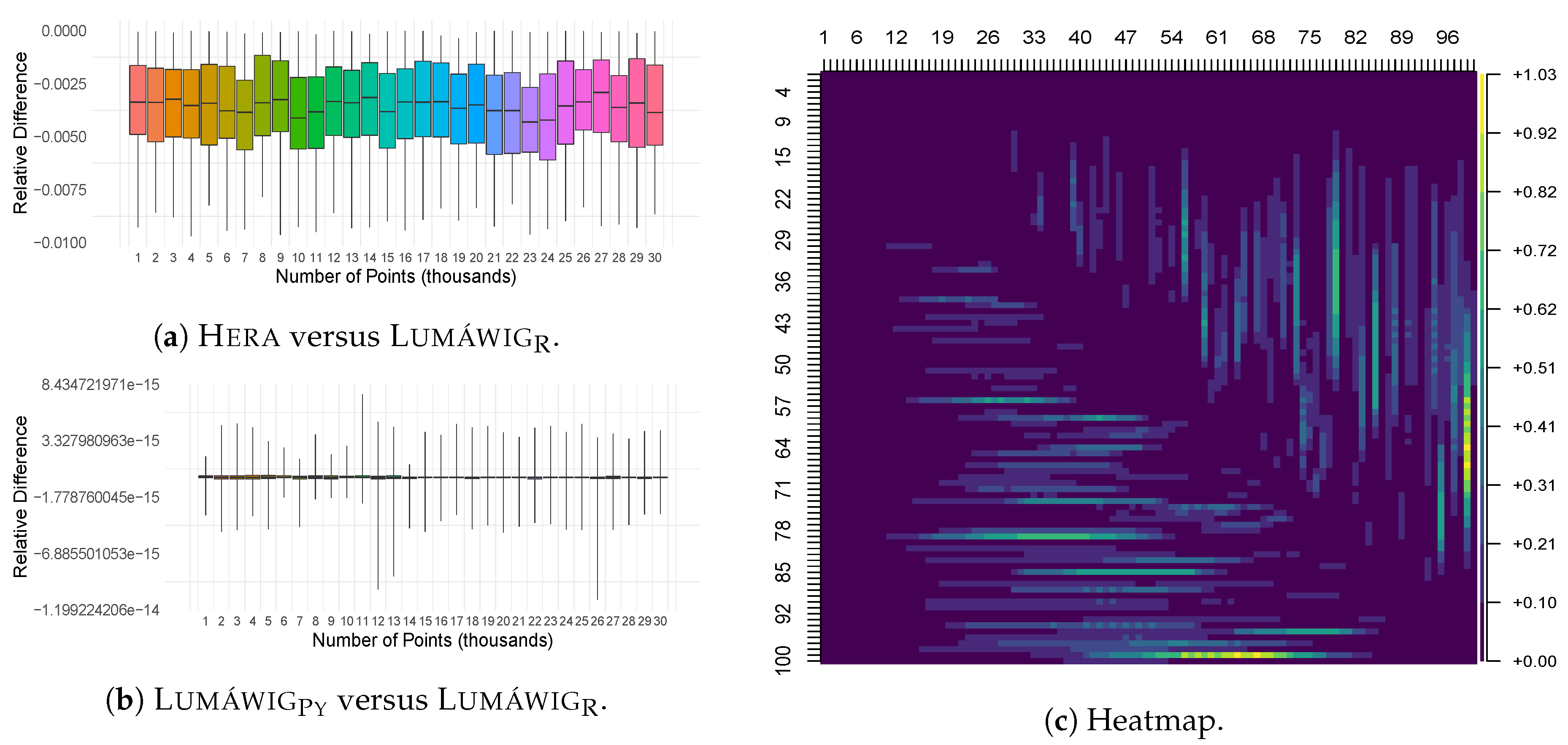
As Lumáwig${}_{\mathsf{R}}$ yields exact values for the bottleneck distance relative to the original Dionysus implementation, we use it as basis in the computation of relative differences in this stage. Figure 6a,b show the relative difference in the computed dimension zero bottleneck distance respectively of Hera and Lumáwig_Py with respect to that of Lumáwig${}_{\mathsf{R}}$. Consistent with the comparison between the outputs of Hera and Dionysus in Figure 4a, Hera consistently overestimates the dimension zero bottleneck distance with respect to that of Lumáwig${}_{\mathsf{R}}$. In contrast, relative differences between the two implementations of Lumáwig can be attributed to rounding differences between Python and R.

3.3. Complexity Analysis

Figure 6c shows a heat map of the median running time of Lumáwig${}_{\mathsf{R}}$ over 100 computations per pixel of the bottleneck distance between pairs of persistence diagram with varying number of points: for $i\le j$, pixel $(i,j)$ represents the median running time for the computation of the bottleneck distance between a diagram with i thousands of points and another diagram with j thousands of points, such that each set of points has death times uniformly chosen from the interval range $(0,2000i)$ and $(0,2000j)$ respectively. It can be inferred from this figure that the best running times happen along the main diagonal, as well as the upper and left portions of the heat map. These correspond to two specific cases: when the diagrams have equal number of points, or when one diagram has overwhelmingly more points than the other. In contrast, regions in the heat map that show increased running times correspond to the case when a diagram that has a large number of points is compared to another that has about half as many points. This observation is supported in the next figure.

Figure 7 shows several scatter plots with fitted curves of the median running times of Lumáwig${}_{\mathsf{R}}$ over 100 computations of dimension zero bottleneck distance. The label in each scatterplot represents the number of points in the fixed base diagram, and a point in the scatterplot at the k thousand mark along the horizontal axis represents the median running time over 100 computations of the bottleneck distance between the base diagram and another diagram with k thousand points whose death times are uniformly chosen from the interval range $(0,2k)$.

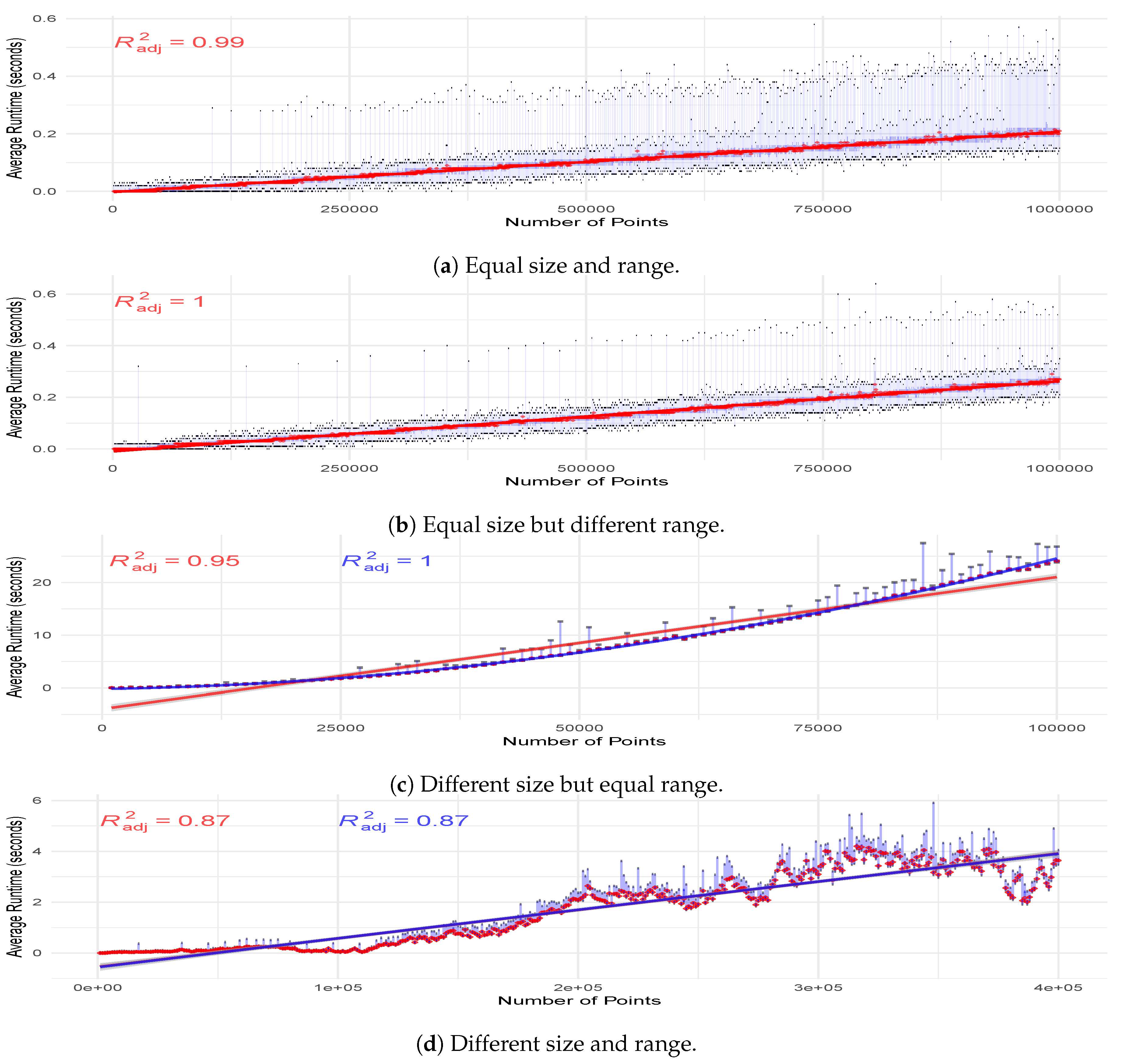
To further investigate the observations above, we examine the performance of Lumáwig${}_{\mathsf{R}}$ in the computation of dimension zero bottleneck distance in four pairs of settings for size of the diagrams and the range of values the death times are drawn from. The first is when Lumáwig${}_{\mathsf{R}}$ is tasked to compare two persistence diagrams with the same number of points whose death times are drawn from the same range of values. We calculate the dimension zero bottleneck distance over 100 pairs of persistence diagrams of equal sizes starting from 1000 to 1,000,000 points. Every diagram is simulated in the same manner as the previous experiments. Median running times are then plotted and fitted with a regression curve. Midspread and range for every 100 computations at every unit of 1000 points are superimposed to illustrate the distribution of running times. Figure 8a shows an excellent linear fit ($R^2=0.99$) for the running time. We also highlight the observed experimental result that the running time between two diagrams each with 1 million points with death times drawn from the range (0, 2,000,000) averages to between 2 and 3 tenths of a second.

The second setting involves two diagrams of the same size but the range of death values for the second is half as wide as the first. In this case, we see in Figure 8b that the running time trend is perfectly fitted with a linear curve. The third setting considers two diagrams where the second has half as many points as the first. We remark that this setting differs from that performed for Figure 6c in that the range where the death times are drawn from for the simulated diagrams in this experiment is the same for the two diagrams.We do this to ensure that any observed significant difference in performance is attributable only to fixed difference in the number of points between the diagrams. As we observe an increased running time for Lumáwig${}_{\mathsf{R}}$ in this case, we compute only to until there are 100,000 points in the larger diagram. Figure 8c shows two fitted regression curves: a quadratic fit with $R^2=1$ and a linear fit with $R^2=0.95$. We highlight that even for the case where Lumáwig${}_{\mathsf{R}}$ evidently takes longer to compute the dimension zero bottleneck distance, a linear model provides a very good fit for the trend.

The final setting is where the second of two diagrams has half as many points with death values drawn from a range half as wide as that for the first. Regression curves are again shown in Figure 8d with linear and quadratic fit both achieving $R^2=0.87$.

4. Lumáwig in Digit Classification

With new access to a fast algorithm for computing dimension zero bottleneck distance, we leverage persistence and other clustering-based diagrams to craft features for digit classification. This application illustrates how the significant computational speed-up for the dimension 0 bottleneck distance affords a way to examine intrinsic differences in the multi-scale clustering dynamics of point clouds from the perspective of persistent homology and in conjuction with hierarchical clustering algorithms. In addition, we will show that information captured by dimension 0 bottleneck distance can be a source of a good feature base for point cloud classification.

We classify 10,000 28 × 28-pixel digit images in the MNIST data set via a random forest classifier. Similar to Garin and Tauzin [16], we train the classifier using features based on topological summaries. However, we depart from Garin and Tauzin’s approach in that we only extract features from dimension zero persistence diagrams and other related clustering-based diagrams. In particular, we craft statistical summaries from distributions of bottleneck distances computed from diagrams resulting from dimension zero persistent homology and clustering of multiple sub-collections of points. It is in this light that the eventual classifier performance must be viewed—the classification of digits, viewed as point clouds with higher dimensional characteristics, is done using lower dimensional clustering information. We summarize this procedure next. For a detailed account of this procedure, we point the interested reader to [21] where it is used to recover higher dimensional shape information of digits from intrinsic clustering behavior.

The first step in the procedure is to generate multiple collections of points from the digits via samples extracted based on point distributions referenced from nine pre-selected landmark points. We use the same landmark points introduced in [16]. Sampling is also done across multiple resolutions by varying the number of points selected in every bin of every distribution histogram. Then, for each sampled sub-collection of points in each sampling resolution, persistent homology and clustering algorithms are respectively used to generate persistence and clustering diagrams. We gather diagrams by their sampling setting and compute pairwise bottleneck distances using Lumáwig. Finally, we compute statistical summaries from the distributions of computed bottleneck distances, and use these to train a random forest classifier with 1000 trees.

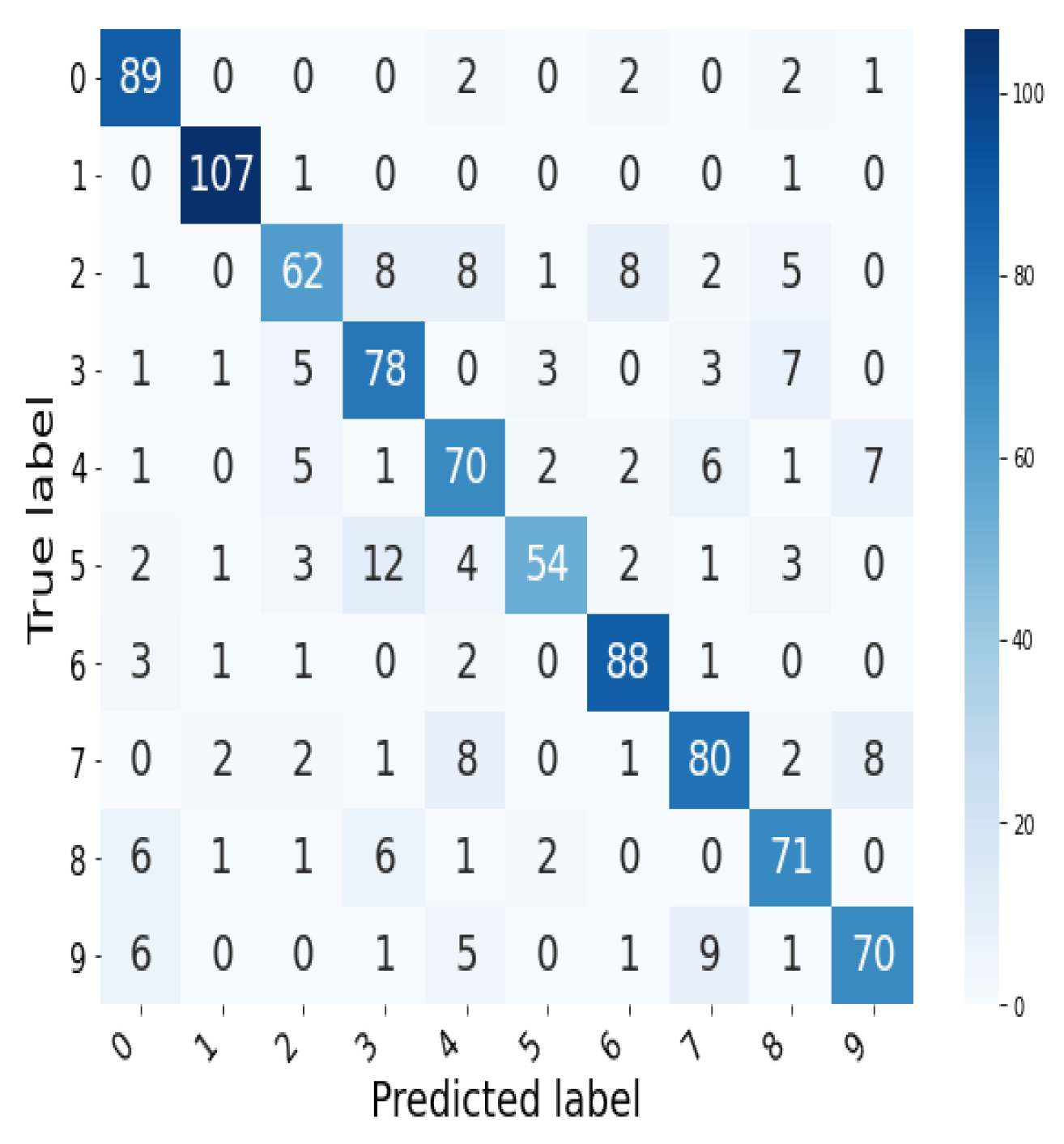
We perform a 10-fold cross validation on our training set of 10,000 digit images from MNIST, and report the summary of obtained $F_1$ scores in

Table 2. Summary of $F_1$ scores on a 10-fold cross validation.

Digit	0	1	2	3	4	5	6	7	8	9	Overall
Mean	0.841	0.940	0.678	0.727	0.687	0.709	0.847	0.754	0.745	0.754	0.768
Std. Dev.	0.030	0.011	0.033	0.019	0.032	0 .037	0.030	0.020	0.015	0.032	0.011

. The average class predictions of the random forest are summarized in the confusion matrix in Figure 9.

The results above show that the random forest classifier is able to use our crafted bottleneck-based features to classify, at a respectable level of accuracy, the 10 digits in the MNIST data set despite all digits possessing the same dimension zero topological signature of having only one connected component. In particular, we infer from the exceptionally high score on the classification of the simplest digit 1, that differences captured by the bottleneck distance in the clustering behavior across multiple point samples of this digit is outstandingly subtle, and hence different, from the rest.

5. Discussions and Conclusions

Our benchmarking experiments reveal that Lumáwig outperforms, by several orders of magnitude, all currently available implementations of dimension zero bottleneck distance in terms of running time. Lumáwig also recovers the exact bottleneck distance produced by Dionysus. We believe this is a significant contribution as it affords a viable tool to process and use dimension zero persistence diagrams in comparing evolving connectivity information between large data sets in a manner that goes beyond the simple use of the most persistent components. Even now, a truly comprehensive and holistic treatment of information embedded in dimension zero persistence diagrams has been left unexplored due primarily to the lack of feasible machinery that can handle significant scaling up in data size. In fact, this note presents the first instance that the bottleneck distance is used in practice for data of magnitude and scale in the order of up to a million. In particular, we see that Lumáwig only takes an average of 2 to 3 tenths of a second to compute the bottleneck distance between diagrams each with one million points.

A natural question to ask is whether a similar strategy of methodically modifying a specific initial bijection to recover all possible cases that yield the best matching for the general case, where birth times of features need not be at the beginning of the filtration (this covers the bottleneck distance for higher dimensional features) is possible. We note that an important first step is to induce an appropriate partial order on the points in each diagram that can accommodate a case-exhaustive approach to optimize the norm. Moreover, the added degree of freedom will naturally introduce cases we have not considered in our optimization step. We are currently exploring generalization strategies that leverage shift-invariant versions of the bottleneck distance due to Cavanna et al. [22].

Our empirical tests suggest that Lumáwig enjoys linear complexity for the case where both diagrams have equal number of points. Moreover, we also see that even for the special case revealed by Figure 7, where there is an apparent slowdown in computational time, the trend seen when data size scales up is also practically linear (see Figure 8c,d). In a future note, we plan to provide a more comprehensive analysis for complexity. Nevertheless, we are confident that Lumáwig can be useful in practical applications of TDA at this stage.

Finally, our application on digit classification showcases, in the same significant way as Weber et al. did in [17], the potential in leveraging persistence diagrams and bottleneck distance as sources of novel features for machine learning tasks. It is our hope that Lumáwig contributes in paving the way for this direction in TDA research.

6. Repository for Lumáwig

Lumáwig will be hosted and maintained in https://github.com/paulsamuelignacio/Lumawig.git as soon as licences (BSD), copyright certificates, and other clearances are secured.

References

- Zomorodian, A. Computing and Comprehending Topology: Persistence and Hierarchical Morse Complexes. Ph.D. Thesis, University of Illinois, Urbana-Champaign, IL, USA, 2001. [Google Scholar]
- Edelsbrunner, H.; Letscher, D.; Zomorodian, A. Topological persistence and simplification. Discrete Comput. Geom. 2002, 28, 511–533. [Google Scholar] [CrossRef] [Green Version]
- Cohen-Steiner, D.; Edelsbrunner, H.; Harer, J. Stability of Persistence Diagrams. Discrete Comput. Geom. 2007, 37, 103–120. [Google Scholar] [CrossRef] [Green Version]
- Morozov, D. Dionysus Library for Computing Persistent. Available online: homology.mrzv.org/software/dionysus (accessed on 2 September 2019).
- Munkres, J. Algorithms for the assignment and transportation problems. J. Soc. Industr. Appl. Math. 1957, 5, 32–38. [Google Scholar] [CrossRef] [Green Version]
- Botnan, M.B.; Lesnick, M. Algebraic stability of zigzag persistence modules. Algebr. Geom. Topol. 2018, 18, 3133–3204. [Google Scholar] [CrossRef]
- Ignacio, P.S.P. Stability of Persistent Directed Clique Homology on Dissimilarity Networks. Ph.D. Thesis, University of Iowa, Iowa City, IA, USA, 2019. [Google Scholar]
- Chowdhury, S.; Mémoli, F. Persistent path homology of directed networks. In Proceedings of the Twenty-Ninth Annual ACM-SIAM Symposium on Discrete Algorithms (SODA ’18), New Orleans, LA, USA, 7–10 January 2018; pp. 1152–1169. [Google Scholar]
- Adcock, A.; Rubin, D.; Carlsson, G. Classification of hepatic lesions using the matching metric. Comput. Vis. Image Underst. 2014, 121, 36–42. [Google Scholar] [CrossRef] [Green Version]
- Seversky, L.; Davis, S.; Berger, M. On Time-Series Topological Data Analysis: New Data and Opportunities. In Proceedings of the IEEE Conference on Computer Vision and Pattern Recognition (CVPR) Workshops, Las Vegas, NV, USA, 26 June–1 July 2016; pp. 59–67. [Google Scholar]
- Chowdhury, S.; Mémoli, F. A functorial Dowker theorem and persistent homology of asymmetric networks. J. Appl. Comput. Topol. 2018, 2, 115–175. [Google Scholar] [CrossRef] [Green Version]
- Bubenik, P. Statistical Topological Data Analysis using Persistence Landscapes. J. Mach. Learn. Res. 2015, 16, 77–102. [Google Scholar]
- Kerber, M.; Morozov, D.; Nigmetov, A. Geometry Helps to Compare Persistence Diagrams. J. Exp. Algorithmicsm 2017, 22, 1–20. [Google Scholar] [CrossRef] [Green Version]
- Efrat, A.; Itai, A.; Katz, M. Geometry Helps in Bottleneck Matching and Related Problems. Algorithmica 2001, 31, 1. [Google Scholar] [CrossRef] [Green Version]
- Hopcroft, J.; Karp, R. An n5/2 algorithm for maximum matchings in bipartite graphs. SIAM J. Comput. 1973, 2, 225–231. [Google Scholar] [CrossRef]
- Garin, A.; Tauzin, G. A Topological “Reading” Lesson: Classification of MNIST using TDA. In Proceedings of the 2019 18th IEEE International Conference On Machine Learning And Applications (ICMLA), Boca Raton, FL, USA, 16–19 December 2019; pp. 1551–1556. [Google Scholar]
- Weber, E.S.; Harding, S.N.; Przybylski, L. Detecting Traffic Incidents Using Persistence Diagrams. Algorithms 2020, 13, 222. [Google Scholar] [CrossRef]
- Belchi, F.; Pirashvili, M.; Conway, J.; Bennett, M.; Djukanovic, R.; Brodzki, J. Lung Topology Characteristics in patients with Chronic Obstructive Pulmonary Disease. Sci. Rep. 2018, 8, 5341. [Google Scholar] [CrossRef] [PubMed]
- Fasy, B.; Kim, J.; Lecci, F.; Maria, C. Introduction to the R package TDA. arXiv 2014, arXiv:1411.1830. [Google Scholar]
- Saul, N.; Tralie, C. Scikit-TDA: Topological Data Analysis for Python. 2019. Available online: https://zenodo.org/record/2533384 (accessed on 9 November 2020). [CrossRef]
- Ignacio, P.S.P. Intrinsic Hierarchical Clustering Behavior Recovers Higher Dimensional Shape Information. arXiv 2010, arXiv:2010.03894. [Google Scholar]
- Cavanna, N.; Kiselius, O.; Sheehy, D. Computing the shift-invariant bottleneck distance for persistence diagrams. In Proceedings of the Canadian Conference on Computational Geometry, Winnipeg, MB, Canada, 8–10 August 2018. [Google Scholar]
Figure 1.
A Rips filtration over a point cloud captures the merging dynamics of clusters evolving from points across multiple scales. The dimension zero persistence diagram produced by this filtration is a set of points positioned along an extended vertical line at the merging heights in the corresponding dendrogram, except for the last point positioned at ∞ representing the eventual single component. The neighborhoods around points are colored by the persistent cluster determined by the elder rule.
Figure 2.
Examples of point-matching between persistence diagrams highlighting the resulting bottleneck distance. Points in each diagrams are shape coded and matched points are color coded. (a) illustrates when diagonal matching achieves the bottleneck distance. (b) is used in the proof of Lemma 1 and (c,d) in Lemma 2.
Figure 3.
Boxplots of running times (seconds in log scale) from different algorithms.
Figure 4.
Boxplots of relative differences from Dionysus of the bottleneck computation outputs in (a) Hera, (b) Persim, (c) LumáwigPy, and (d) Lumáwig.
Figure 5.
Running time (seconds in log scale) of Lumáwig versus the current state-of-the-art implementation in Hera. Five boxplots for the running time of the original algorithm in Dionysus are superimposed for reference.
Figure 6.
(a,b) Boxplots of relative differences between the bottleneck computation outputs of the indicated pair of implementations. (c) Heat map of the median running times of Lumáwig. Each pixel represents the median running time (in seconds) for 100 computations of dimension zero bottleneck distance between diagrams. The number of points in the diagrams are in units of 1000.
Figure 7.
Scatter plots with fitted curves of the median running times (in seconds) of Lumáwig over 100 computations of dimension zero bottleneck distance between a base diagram with the labeled number of points and a diagram with k thousands of points, for .
Figure 8.
Median running time in the computation of bottleneck distance between two diagrams with varying size and range settings fitted with regression curves. Superimposed are the minimum and maximum running times over the 100-run simulation per unit of 1000 points to illustrate the running time range, and the narrow darker blue band to show the midspread.
Figure 9.
Confusion matrix for the average prediction of the random forest over a 10-fold cross validation.