Spectrum-Adapted Polynomial Approximation for Matrix Functions with Applications in Graph Signal Processing


1
Institute for Computational & Mathematical Engineering, Stanford University, Stanford, CA 94305, USA
2
Department of Mathematics, Statistics, and Computer Science, Macalester College, St. Paul, MN 55105, USA
3
IBM T.J. Watson Research Center, Yorktown Heights, NY 10598, USA
4
Department of Computer Science and Engineering, University of Minnesota, Minneapolis, MN 55455, USA
*
Author to whom correspondence should be addressed.
Algorithms 2020, 13(11), 295; https://0-doi-org.brum.beds.ac.uk/10.3390/a13110295
Submission received: 16 October 2020
/
Revised: 16 October 2020
/
Accepted: 29 October 2020
/
Published: 13 November 2020
(This article belongs to the Special Issue Efficient Graph Algorithms in Machine Learning)
Abstract
:We propose and investigate two new methods to approximate for large, sparse, Hermitian matrices . Computations of this form play an important role in numerous signal processing and machine learning tasks. The main idea behind both methods is to first estimate the spectral density of , and then find polynomials of a fixed order that better approximate the function f on areas of the spectrum with a higher density of eigenvalues. Compared to state-of-the-art methods such as the Lanczos method and truncated Chebyshev expansion, the proposed methods tend to provide more accurate approximations of at lower polynomial orders, and for matrices with a large number of distinct interior eigenvalues and a small spectral width. We also explore the application of these techniques to (i) fast estimation of the norms of localized graph spectral filter dictionary atoms, and (ii) fast filtering of time-vertex signals.
1. Introduction
Efficiently computing , a function of a large, sparse Hermitian matrix times a vector, is an important component in numerous signal processing, machine learning, applied mathematics, and computer science tasks. Application examples include graph-based semi-supervised learning methods [1,2,3]; graph spectral filtering in graph signal processing [4]; convolutional neural networks/deep learning [5,6]; clustering [7,8]; approximating the spectral density of a large matrix [9]; estimating the numerical rank of a matrix [10,11]; approximating spectral sums such as the log-determinant of a matrix [12] or the trace of a matrix inverse for applications in physics, biology, information theory, and other disciplines [13]; solving semidefinite programs [14]; simulating random walks [15] (Chapter 8); and solving ordinary and partial differential equations [16,17,18].
References [19] (Chapter 13), [20,21,22] survey different approaches to this well-studied problem of efficiently computing
where the columns of are the eigenvectors of the Hermitian matrix ; is a diagonal matrix whose diagonal elements are the corresponding eigenvalues of , which we denote by ; and is a diagonal matrix whose kth diagonal entry is given by . For large matrices, it is not practical to explicitly compute the eigenvalues of in order to approximate (1). Rather, the most common techniques, all of which avoid a full eigendecomposition of , include (i) truncated orthogonal polynomial expansions, including Chebyshev [23,24,25] and Jacobi; (ii) rational approximations [21] (Section 3.4); (iii) Krylov subspace methods such as the Lanczos method [23,26,27,28,29]; and (iv) quadrature/contour integral methods [19] (Section 13.3).
Our focus in this work is on polynomial approximation methods. Let be a degree K polynomial approximation to the function f on a known interval containing all of the eigenvalues of . Then the approximation can be computed recursively, either through a three-term recurrence for specific types of polynomials (see Section 3 for more details), or through a nested multiplication iteration [30] (Section 9.2.4), letting , and then iterating
The computational cost of either of these approaches is dominated by multiplying the sparse matrix by K different vectors. The approximation error is bounded by
If, for example, is a degree K truncated Chebyshev series approximation of an analytic function f, the upper bound in () converges geometrically to 0 as K increases, at a rate of , where is the radius of an open Bernstein ellipse on which f is analytic and bounded (see, e.g., [31] (Theorem 5.16), [32] (Theorem 8.2)).
In addition to the computational efficiency and convergence guarantees, a third advantage of polynomial approximation methods is that they can be implemented in a distributed setting [33]. A fourth advantage is that the ith element of only depends on the elements of within K hops of i on the graph associated with (e.g., if is a graph Laplacian matrix, a nonzero entry in the th element of , where , corresponds to an edge connecting vertices i and j in the graph). This localization property is important in many graph-based data analysis applications, such as graph spectral filtering [34] and deep learning [5]. Finally, as opposed to other methods that incorporate prior knowledge about into the choice of the approximating polynomial (e.g., [35] considers vectors from a zero-mean distribution with a known covariance matrix), the polynomial approximations resulting from the methods we propose do not depend on or any information about . Thus, in applications where the computation of is repeated for many different vectors with the same f and , the polynomial coefficients only need to be computed a single time.
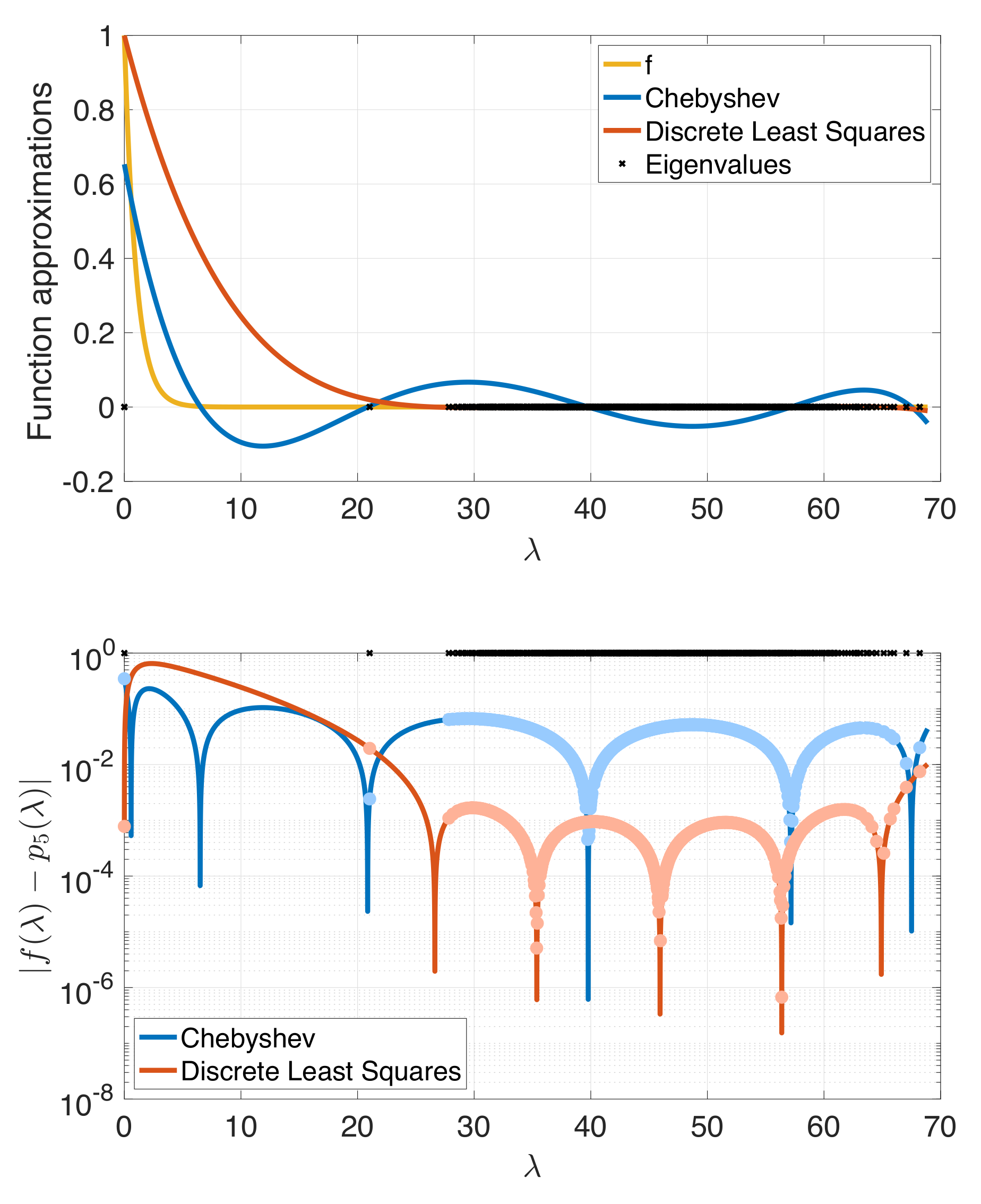
While the classical truncated orthogonal polynomial expansion methods (e.g., Chebyshev, Legendre, Jacobi) aim to approximate the function f throughout the full interval , it is only the polynomial approximation error at the eigenvalues of that affects the overall error in (3). With knowledge of the complete set of eigenvalues, we could do better, for example, by fitting a degree K polynomial via the discrete least squares problem . In Figure 1, we show an example of such a discrete least squares fitting. The resulting approximation error for is 0.020, as opposed to 0.347 for the degree 5 truncated Chebyshev approximation. This is despite the fact that is equal to 0.650 for the discrete least squares approximation, as opposed to 0.347 for the Chebyshev approximation.
While in our setting we do not have access to the complete set of eigenvalues, our approach in this work is to leverage recent developments in efficiently estimating the spectral density of the matrix , to adapt the polynomial to the spectrum in order to achieve better approximation accuracy at the (unknown) eigenvalues. After reviewing spectral density estimation in the next section, we present two new classes of spectrum-adapted approximation techniques in Section 3. In Section 4, we perform numerical experiments, approximating for different matrices and functions f, and discuss the situations in which the proposed methods work better than the state-of-the-art methods. In Section 5 and Section 6, we explore the application of the proposed technique to fast estimation of the norms of localized graph spectral filter dictionary atoms and fast filtering of time-vertex signals, respectively.
2. Spectral Density Estimation
The cumulative spectral density function or empirical spectral cumulative distribution of the matrix is defined as
where if statement C is true and otherwise. The spectral density function [36] (Chapter 6) (also called the Density of States or empirical spectral distribution [37] (Chapter 2.4)) of is the probability measure defined as
Lin et al. [9] provide an overview of methods to approximate these functions. In this work, we use a variant of the Kernel Polynomial Method (KPM) [38,39,40] described in [9,41] to estimate the cumulative spectral density function of . Namely, for each of S linearly spaced points between and , we estimate the number of eigenvalues less than or equal to via stochastic trace estimation [42,43]. Let denote a Gaussian random vector with distribution , denote a sample of size J from this distribution, and denote a Jackson–Chebyshev polynomial approximation to [44,45]. The stochastic trace estimate of the number of eigenvalues less than or equal to is then given by
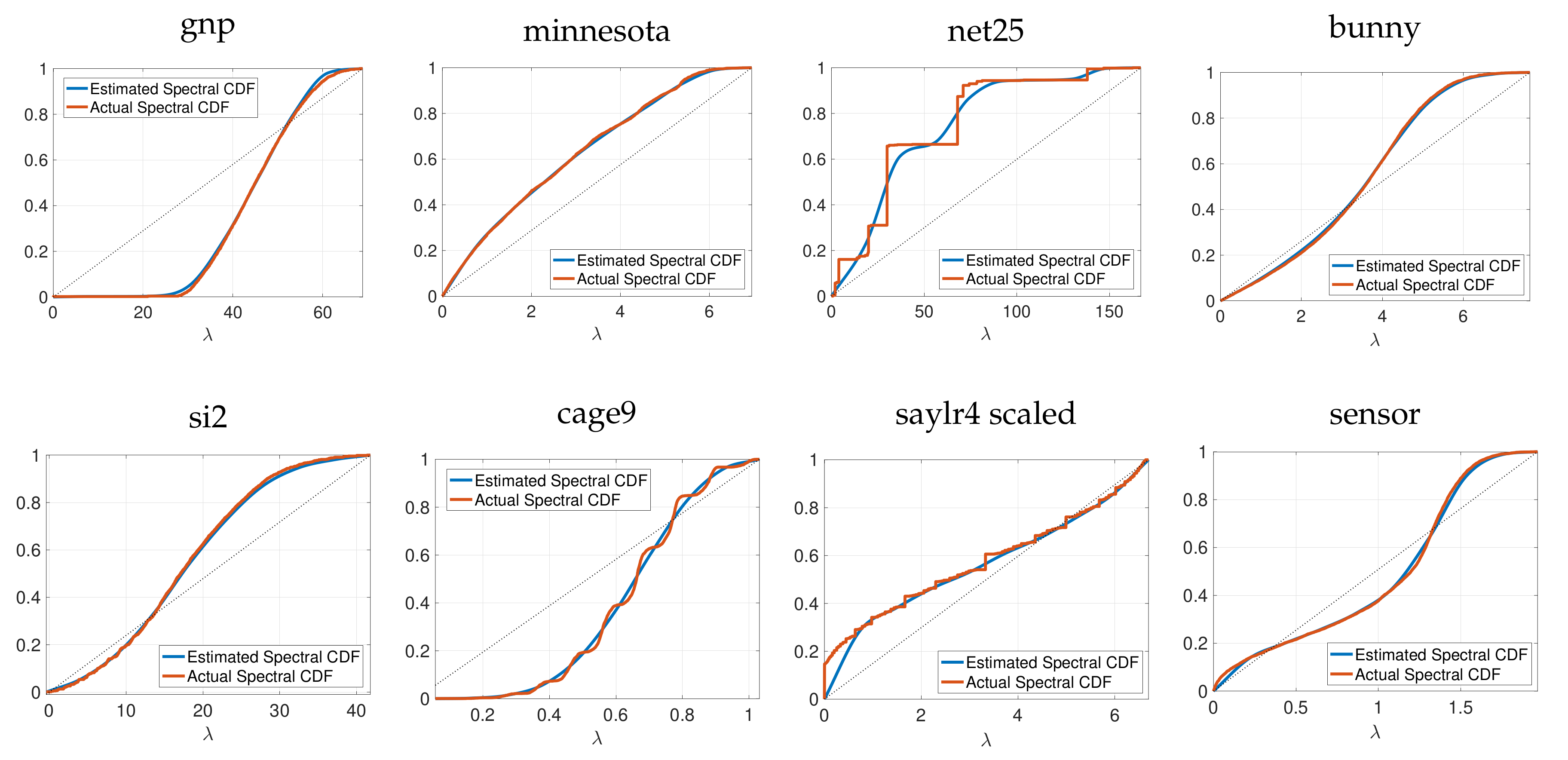
As in [46], we then form an approximation to by performing monotonic piecewise cubic interpolation [47] on the series of points . Analytically differentiating yields an approximation to the spectral density function . Since is a monotonic cubic spline, we can also analytically compute its inverse function . The spectrum-adapted methods we propose in Section 3 utilize both and to focus on regions of the spectrum with higher eigenvalue density when generating polynomial approximations. Figure 2 shows examples of the estimated cumulative spectral density functions for eight real, symmetric matrices : the graph Laplacians of the Erdös–Renyi graph (gnp) from Figure 1, the Minnesota traffic network [48] (), and the Stanford bunny graph [49] (); the normalized graph Laplacian of a random sensor network () from [50]; and the net25 (), si2 (), cage9 (), and saylr4 () matrices from the SuiteSparse Matrix Collection [51] (We use for cage9, and for net25 and saylr4, we generate graph Laplacians based on the off-diagonal elements of . For saylr4, we scale the entire Laplacian by a factor of ).
The computational complexity of forming the estimate is , where M is the number of nonzero entries in , J is the number of random vectors in (6) (in our experiments, suffices), and is the degree of the Jackson–Chebyshev polynomial approximations [41]. While this cost is non-negligible if computing for a single f and a single , it only needs to be computed once for each if repeating this calculation for multiple functions f or multiple vectors , as is often the case in the applications mentioned above.
3. Spectrum-Adapted Methods
In this section, we introduce two new classes of degree K polynomial approximations to , both of which leverage the estimated cumulative spectral density function .
3.1. Spectrum-Adapted Polynomial Interpolation
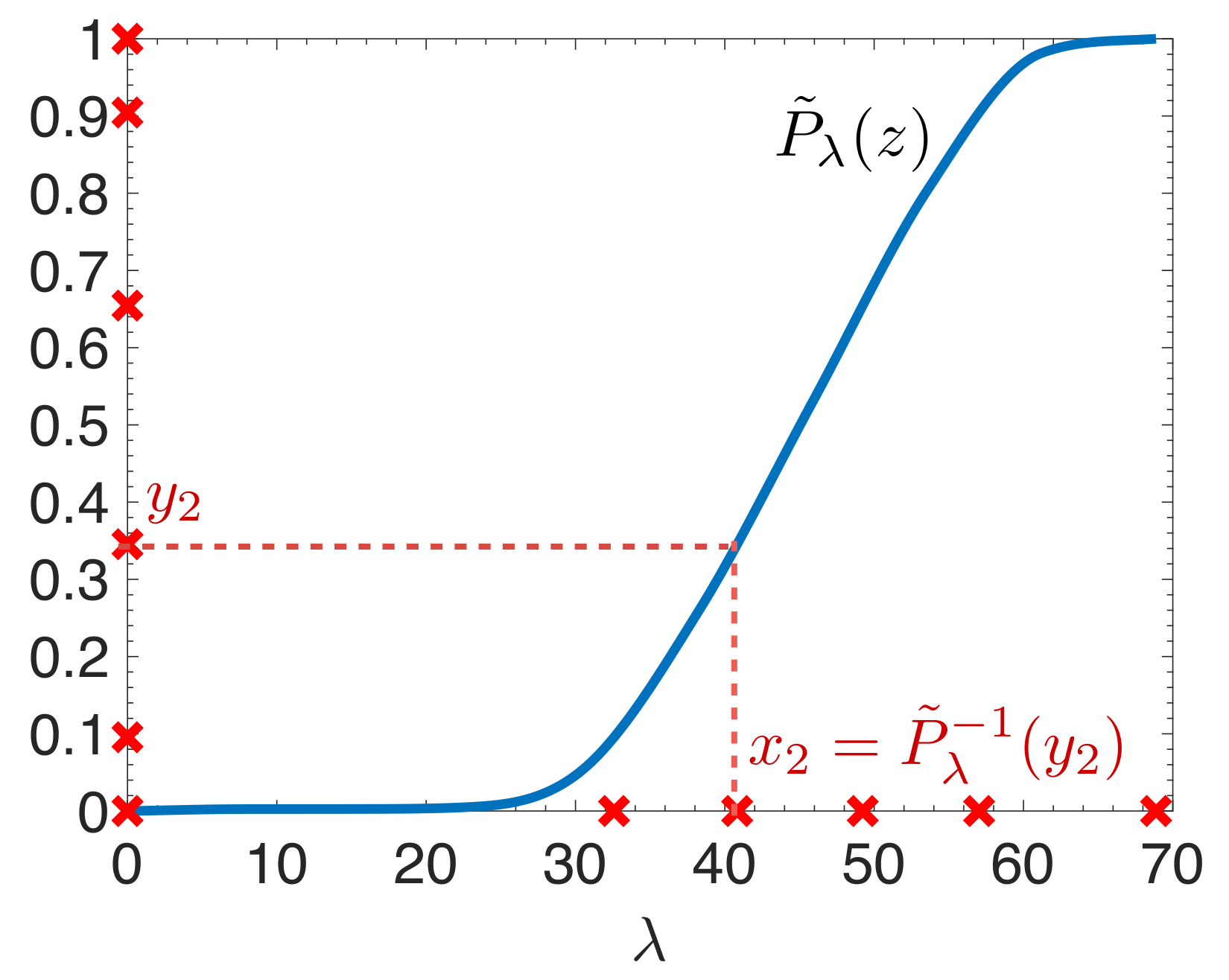
In the first method, we take , for , which are the extrema of the degree K Chebyshev polynomial shifted to the interval . We then warp these points via the inverse of the estimated cumulative spectral density function by setting , before finding the unique degree K polynomial interpolation through the points . The intuition behind warping the interpolation points is that (i) a better approximation is attained in areas of the spectrum (domain) with more interpolation points, (ii) the error in (3) only depends on the errors at the eigenvalues of A, so we would like the approximation to be best in regions with many eigenvalues, and (iii) as shown in Figure 3, using the inverse of the estimated cumulative spectral density function as the warping function leads to a higher density of the warped points falling in higher density regions of the spectrum of . Thus, the warping should ideally lead to more interpolation points in high density regions of the spectrum, better approximation of the target function in these regions, and, in turn, a reduction in the error (3), as compared to interpolations generated from points spread more evenly across the spectrum.
To find the (unique) degree K polynomial interpolation, our numerical implementation uses MATLAB’s polyfit function, which centers and scales the data and then solves the resulting system of equations via a QR decomposition. Once the interpolating polynomial coefficients are attained, can be computed, e.g., via (2) or by representing the interpolating polynomial as a linear combination of Chebyshev polynomials and using Chebyshev coefficients in the associated three-term recurrence [23,32]. This entire procedure is detailed in Algorithm 1.
| Algorithm 1 Spectrum-adapted polynomial interpolation. |
| Input Hermitian matrix , vector , function f, polynomial degree K |
| Output degree K approximation |
|
3.2. Spectrum-Adapted Polynomial Regression/Orthogonal Polynomial Expansion
A second approach is to solve the weighted least squares polynomial regression problem
where the abscissae and weights are chosen to capture the estimated spectral density function. We investigated several methods to set the points (e.g., linearly spaced points, Chebyshev points on the interval , Chebyshev points on each subinterval , and warped points via the inverse of the estimated cumulative spectral density function as in Section 3.1) and weights (e.g., the analytically computed estimate of the spectral density function, a discrete estimate of the spectral density function based on the eigenvalue counts in (6), the original KPM density of states method based on a truncated Chebyshev expansion [9] (Equation 3.11), or equal weights for warped points). Without going into extensive detail about these various options, we remark that choosing abscissae that are very close to each other, which may occur when using points warped by the inverse of the estimated density function, may lead to numerical instabilities when solving the weighted least squares problem. In the numerical experiments, we use M evenly spaced points on the interval (i.e., ), and set the weights to be . To solve (7), we use a customized variant of MATLAB’s polyfit function that solves, again via QR decomposition, the normal equations of the weighted least squares problem:
where is the Vandermonde matrix associated with the points , is a diagonal matrix with diagonal elements equal to the weights , is a column vector with entries equal to , and is the vector of unknown polynomial coefficients. Once the coefficients of the optimal polynomial, are attained, can once again be computed, e.g., via (2). A summary of this method is detailed in Algorithm 2 (As pointed out by an anonymous reviewer, since our estimate of the spectral density function is a piecewise quadratic function, the optimization problem (7) could be replaced by its continuous analog, , which can be solved analytically for many functions ).
| Algorithm 2 Spectrum-adapted polynomial regression. |
| Input Hermitian matrix , vector , function f, polynomial degree K, number of grid points M |
| Output degree K approximation |
|
An alternative way to view this weighted least squares method [52] is as a truncated expansion in polynomials orthogonal with respect to the discrete measure with finite support at the points , and an associated inner product [53] (Section 1.1)
The M discrete monic orthogonal polynomials satisfy the three-term recurrence relation [53] (Section 1.3)
with , , ,
Given the abscissae and weights , the three-term recursion coefficients and can also be computed through a stable Lanczos type algorithm on an matrix [53] (Section 2.2.3), [54]. In matrix-vector notation, the vectors , which are the discrete orthogonal polynomials evaluated at the M abscissae, can be computed iteratively by the relation
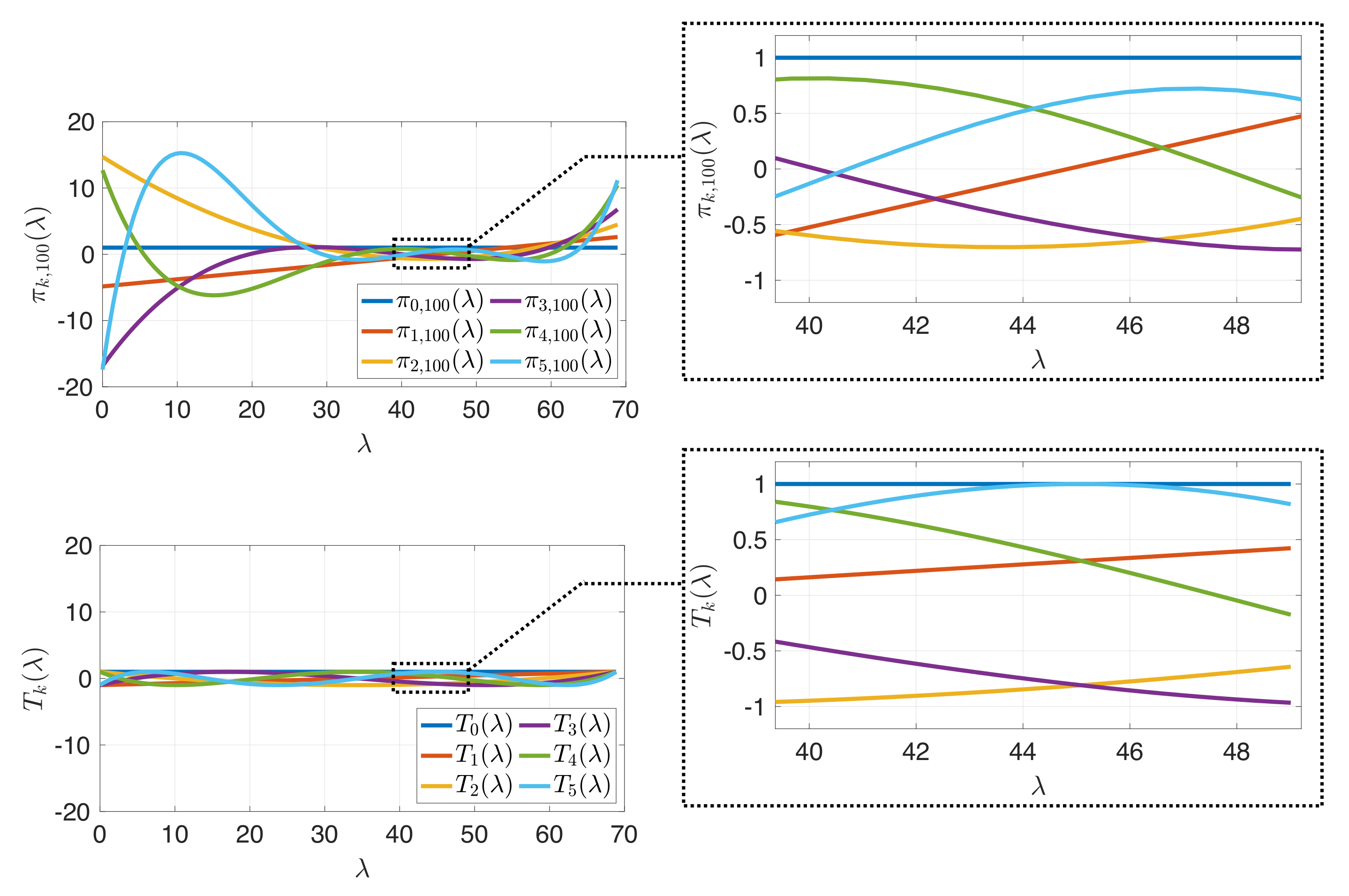
with and . Figure 4 shows an example of these discrete orthogonal polynomials.
Finally, the degree K polynomial approximation to is computed as
with , , and
Before proceeding to numerical experiments, we briefly comment on the relationship between the spectrum-adapted approximation proposed in this section and the Lanczos approximation to , which is given by [19] (Section 13.2), [23]
where is an matrix whose columns form an orthonormal basis for , a Krylov subspace. In (9), is a tridiagonal Jacobi matrix. The first column of is equal to . The approximation (9) can also be written as , where is the degree K polynomial that interpolates the function f at the eigenvalues of [19] (Theorem 13.5), [55]. Thus, unlike classical polynomial approximation methods, such as the truncated Cheybshev expansion, the Lanczos method is indirectly adapted to the spectrum of . The Lanczos method differs from proposed method in that and the Lanczos approximating polynomial depend on the initial vector . Specifically, the polynomials generated from the three-term recurrence of the form (8)
with the and coefficients taken from the diagonal and superdiagonal entries of , respectively, are orthogonal with respect to the piecewise-constant measure
where , and is its jth component [56] (Theorem 4.2). If happens to be a constant vector, then from (5). If is a graph Laplacian, is the graph Fourier transform [4] of , normalized to have unit energy.
4. Numerical Examples and Discussion
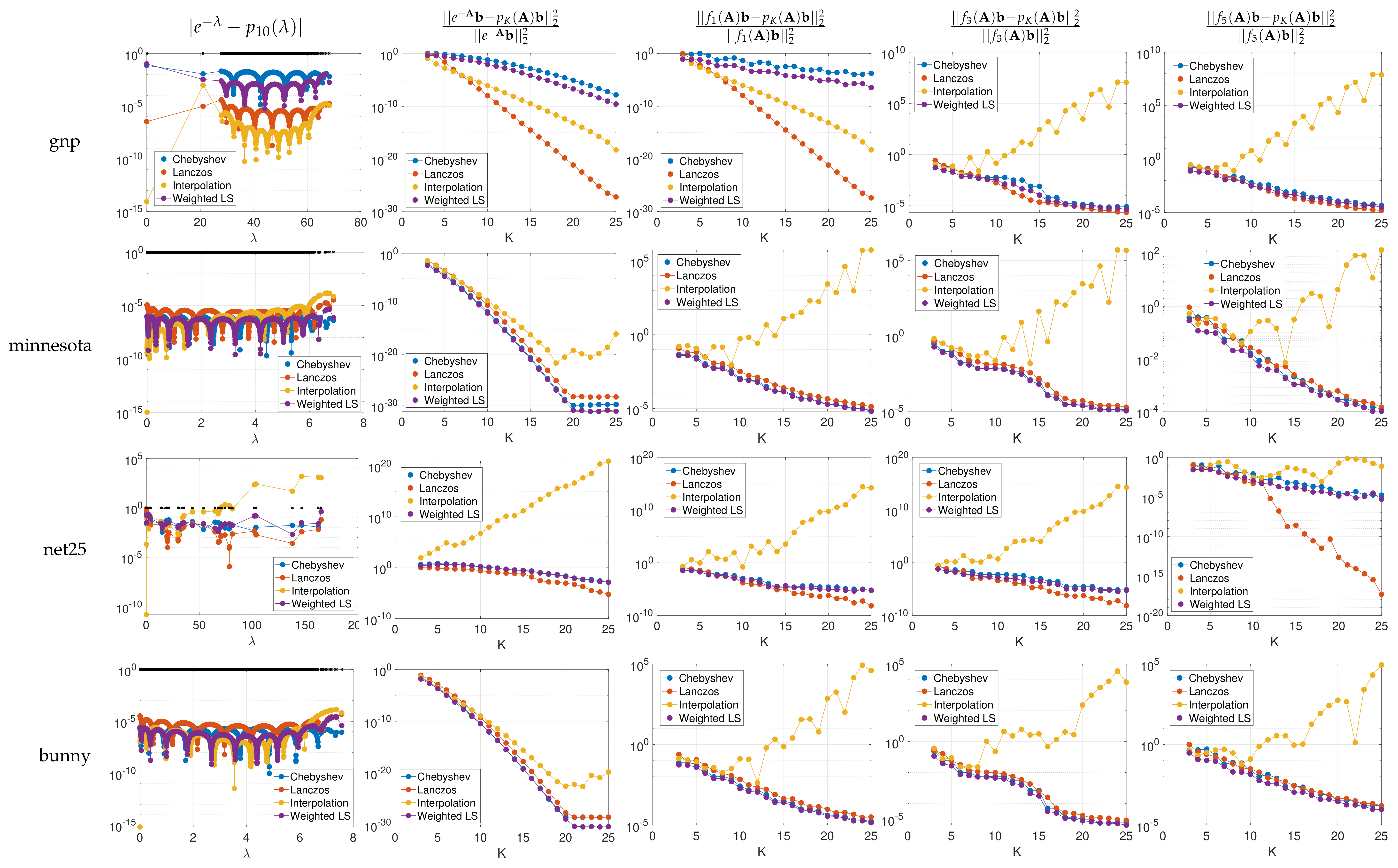
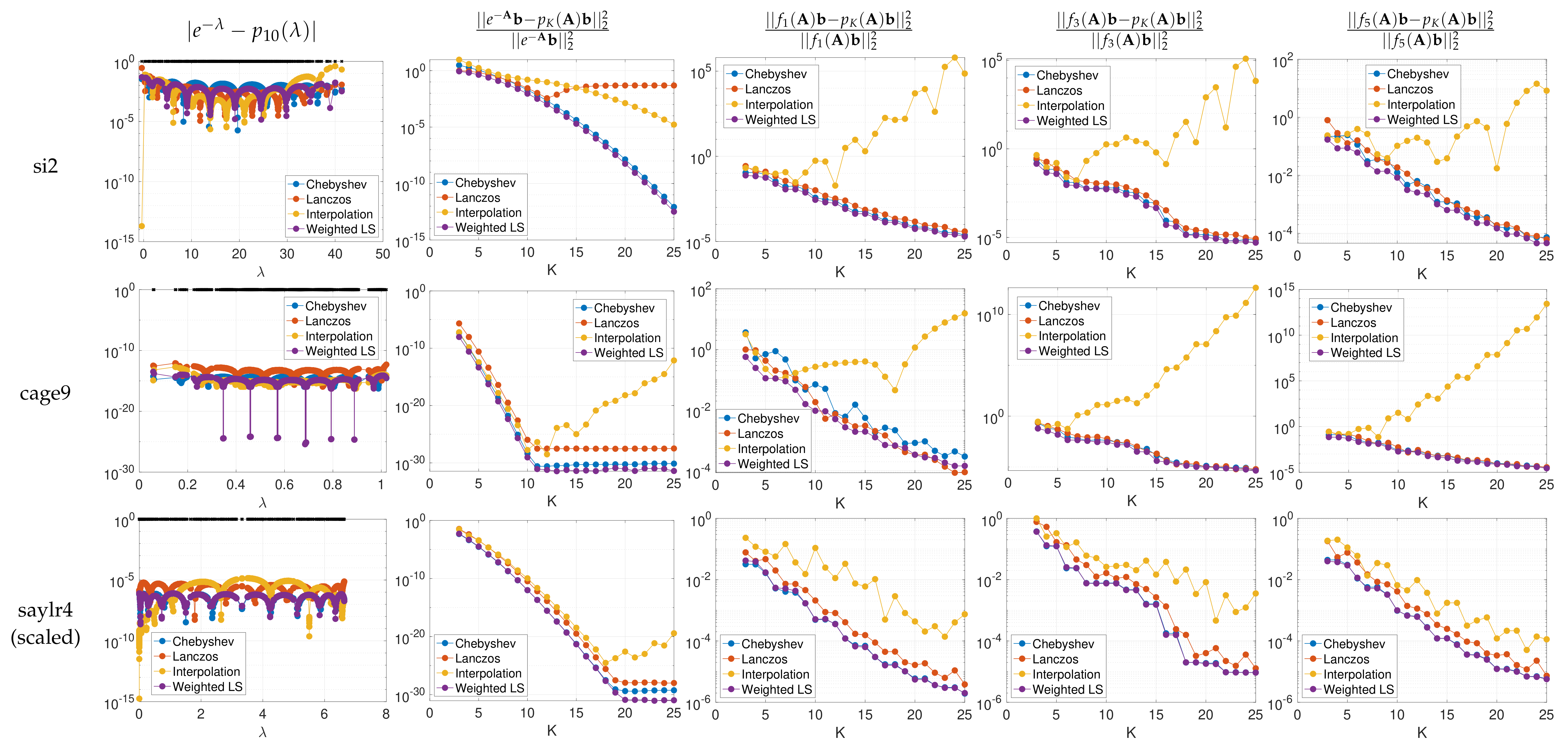
In Figure 5, for different functions and matrices , we approximate with and polynomial approximation orders ranging from to 25. To estimate the cumulative spectral density function with parameters , , and , we use the KPM, as shown in Figure 2. Based on the analytical derivative and inverse function of , we obtain the two proposed spectrum-adapted polynomial approximations for , before computing each via the corresponding three-term recursion. We compare the proposed methods to the truncated Chebyshev expansion and the Lanczos method with the same polynomial order. Note that when is a constant vector in the spectral domain of , the relative error is equal to , the numerator of which is the discrete least squares objective mentioned in Section 1. The first column of Figure 5 displays the errors at all eigenvalues of for each order 10 polynomial approximation of . The second column examines the convergence of relative errors in approximating for matrices with various spectral distributions, for each of the four methods.
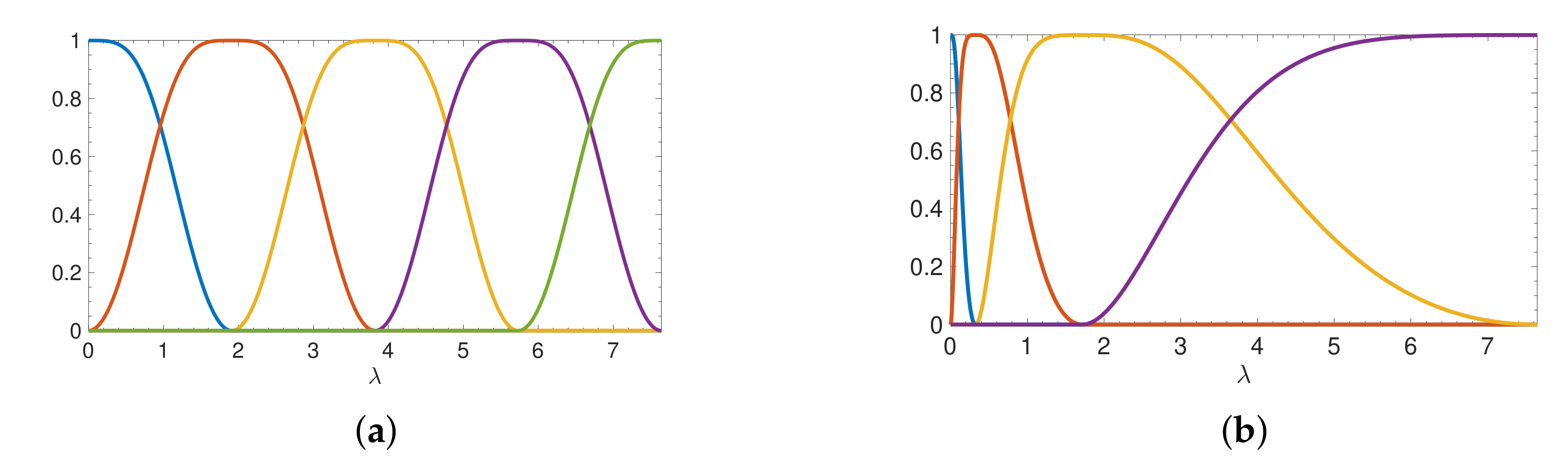
In the field of graph signal processing [4], it is common to analyze or modify a graph signal , where is the value of the graph signal at vertex i of a weighted, connected graph G with N vertices, by applying a graph spectral filter . The filtered signal is exactly the product (1) of a function of the graph Laplacian (or some other symmetric matrix) and a vector, the graph signal . In Figure 6, we show examples of collections of such functions, commonly referred to as graph spectral filter banks. In the right three columns of Figure 5, we examine the relative errors incurred by approximating for the lowpass, bandpass, and highpass graph spectral filters , , and shown in Figure 6a. We expand on the applications of such graph spectral filters in Section 5.
We make two observations based on the numerical examples:
- The spectrum-adapted interpolation method often works well for low degree approximations (), but is not very stable at higher orders due to overfitting of the polynomial interpolant to the specific interpolation points (i.e., the interpolant is highly oscillatory).
- The proposed spectrum-adapted weighted least squares method tends to outperform the Lanczos method for matrices such as si2 and cage9 that have a large number of distinct interior eigenvalues.
5. Application I: Estimation of the Norms of Localized Graph Spectral Filter Dictionary Atoms
A common method to extract information from data residing on a weighted, undirected graph is to represent the graph signal as a linear combination of building block graph signals called atoms, a collection of which is called a dictionary. In this section, we consider localized spectral graph filter dictionaries with the form , where each atom is defined as with being the graph Laplacian and having a value of 1 at vertex i and 0 elsewhere. Each atom can be interpreted as the result of localizing a spectral pattern characterized by the filter function to be centered at vertex i in the graph. See [58] for more details about localized spectral graph filter dictionaries and their applications as transforms and regularizers in myriad signal processing and machine learning tasks.
For large, sparse graphs, the dictionary atoms are never explicitly computed; rather, their inner products with the graph signal are approximated by , using polynomial approximation methods such as those described in Section 1 or those proposed in this work. However, in graph signal processing applications such as thresholding for denoising or compression [58,59,60] or non-uniform random sampling and interpolation of graph signals [41,45,58,61], it is often important to form a fast estimate of the norms of the dictionary atoms, . Since is a bilinear form of the type , the norm of a single atom can be estimated via quadrature methods such as Lanczos quadrature [53] (Ch. 3.1.7), [56] (Ch. 7), [62]; however, doing this for all atoms is not computationally tractable since each requires a different combination of function and starting vector. Other alternatives include the methods discussed in [63] for estimating diagonal elements of a matrix that is not explicitly available but for which matrix-vector products are easy to evaluate, as .
In this application example, we estimate the norms of the dictionary atoms through the products of matrix functions with random vectors, as follows. Let be a random vector with each component having an independent and identical standard normal distribution (in fact, we are only utilizing the property that the random components have unit variance). Then we have
Thus, to estimate , it suffices to estimate for a degree K polynomial approximation to . We therefore define each atom norm estimate as the sample standard deviation
where each is a realization of the random vector . In the numerical experiments, we compare the estimates resulting from Chebyshev polynomial approximation to those resulting from spectrum-adapted weighted least squares polynomial approximation. As a computational aside, in the process of estimating the spectral density via KPM in (6), we have already computed for each and each j, where are the Chebyshev polynomials shifted to the interval . From these quantities, we can easily compute the vectors in (10) for different values of l (different filters). See [41] (Sec. III.B.1) for details.
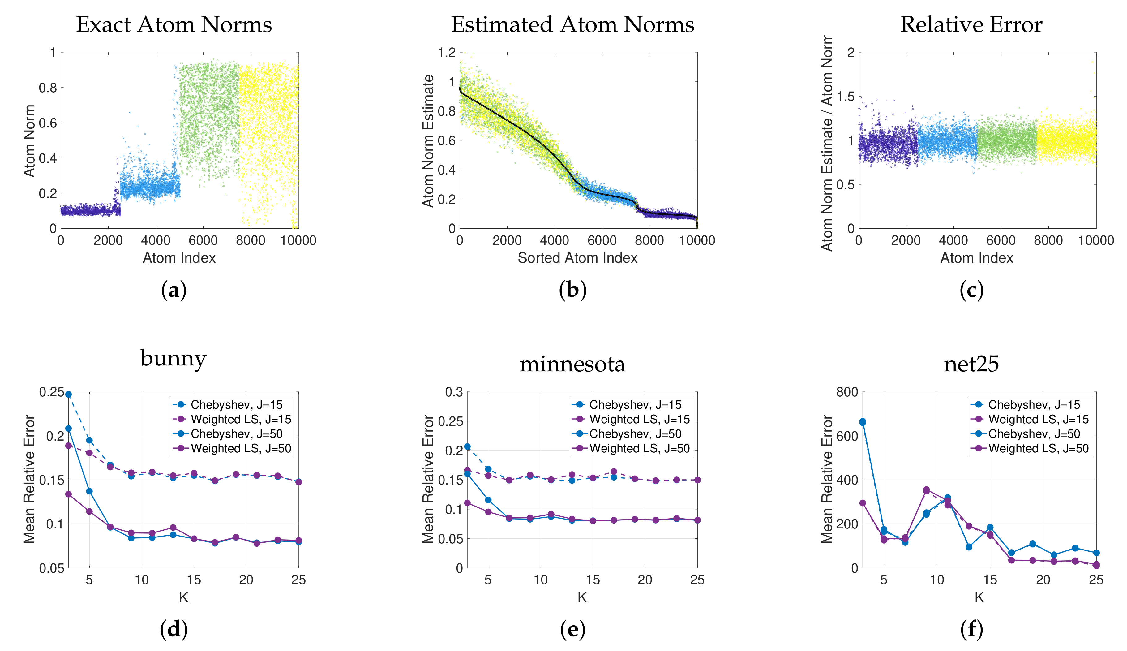
In the top row of Figure 7, we demonstrate the estimation of the norms of the atoms of a spectral graph wavelet dictionary generated by localizing the four filters in Figure 6b to each of the vertices of the bunny graph. Figure 7a shows the exact norms of the dictionary atoms. In Figure 7b, we plot the estimated norms of the atoms, generated via degree spectrum-adapted weighted least squares polynomial approximation with random vectors in (10), against the actual atom norms. The ratios of the estimated atom norms to the actual norms are shown in Figure 7c. We show the mean of the relative error across all of these atoms as a single point in Figure 7d, and also repeat this experiment with different values of K and J and different classes of approximating polynomials, as well as for different graphs in Figure 7e–f. On all three graphs and at both values of J, for low degrees K, the estimates generated from the spectrum-adapted polynomial least squares method have lower mean relative error than those based on Chebyshev polynomial approximation. While these examples are on small to medium graphs for comparison to the exact atom norms, the method scales efficiently to dictionaries designed for large, sparse graphs.
6. Application II: Fast Filtering of Time-Vertex Signals
In this section, we demonstrate the use of the spectrum-adapted approximation methods in Section 3 to accelerate the the joint filtering of time-vertex signals in both time and graph spectral domains [50,64,65].
6.1. Time-Vertex Signals
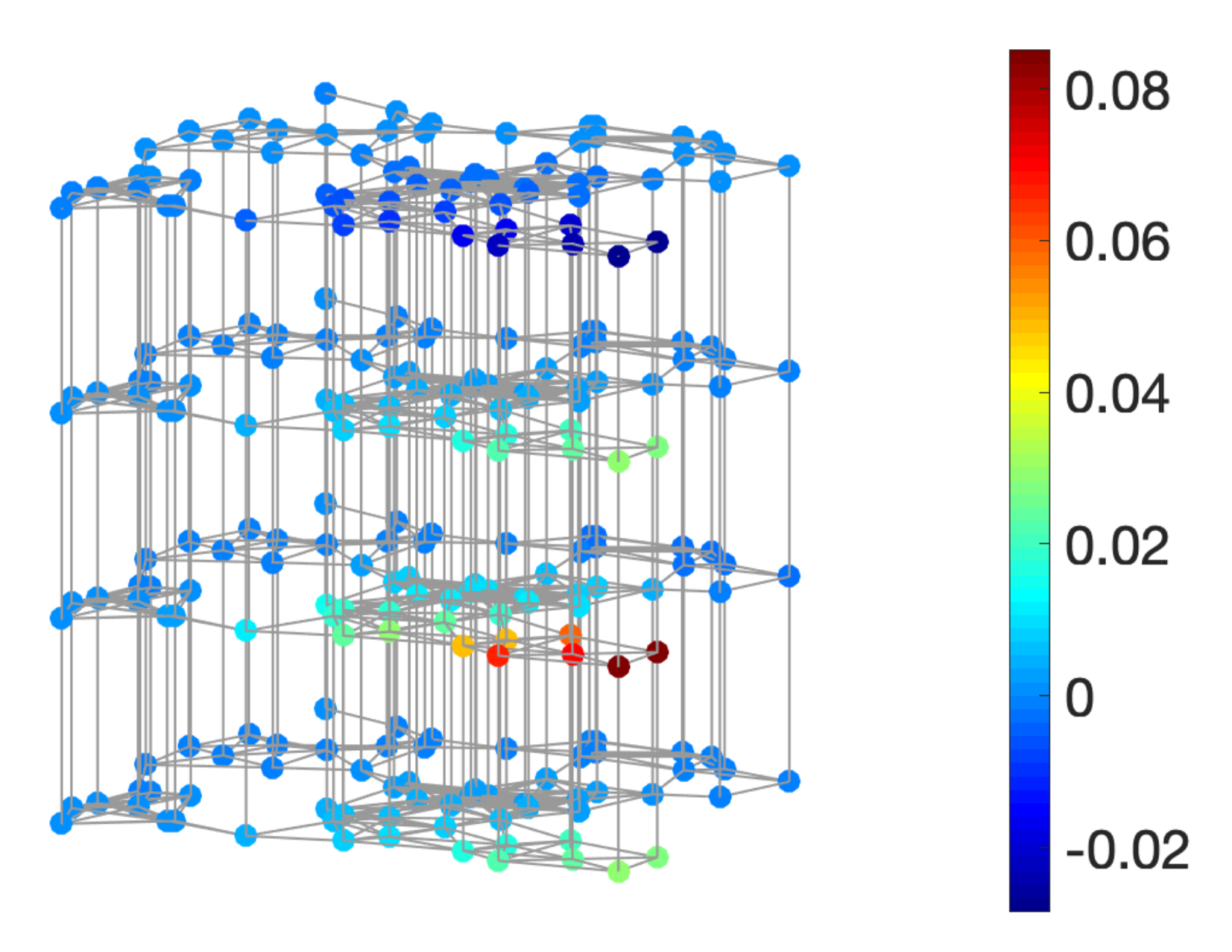
We consider a weighted, undirected graph with N vertices, where is the set of vertices, is the set of edges, and is the weighted adjacency matrix. The combinatorial graph Laplacian is defined as , where is diagonal with equal to the degree of the ith vertex. At each vertex, we observe a time series of T observations. Thus, the time-varying graph signal can be represented as a matrix , where is the value on the ith vertex at the jth time. Figure 8 shows an example of a time-vertex signal.
6.2. Time-Vertex Filtering
Fixing a point in time, each column of is a graph signal defined on G. Let denote the jth column of , . Based on the graph structure of G, we can perform high-dimensional graph signal processing tasks on , such as filtering, denoising, inpainting, and compression [4]. In particular, for a filter defined on the eigenvalues of , the graph spectral filtering of can be computed as , where is the conjugate transpose of , and is the spectral decomposition of .
Conversely, focusing on one vertex of G, the ith row of is a discrete time signal , which indicates how the signal value changes over time on the ith vertex. We can compute the one-dimensional discrete Fourier transform (DFT) of by , where is the normalized DFT matrix of size T, and is its complex conjugate. The DFT converts a signal from the time domain to the frequency domain, and allows for the amplification or attenuation of different frequency components of the signal. This process is referred to as frequency filtering in classical signal processing [4]. Frequency filtering of classical one-dimensional signals is equivalent to graph spectral filtering of graph signals on a ring graph [66] (Theorem 5.1). Let denote the graph Laplacian of a ring graph with T vertices. Its spectral decomposition gives , where comprises the DFT basis vectors (normalized to have length 1), and the eigenvalue is given by , for .
The joint time-vertex Fourier transform of a time-varying graph signal is defined as the combination of a graph Fourier transform and a DFT [50]:
A joint time-vertex filter is defined for all combinations of where is an eigenvalue of and is an eigenvalue of . The joint time-vertex filtering is defined accordingly as
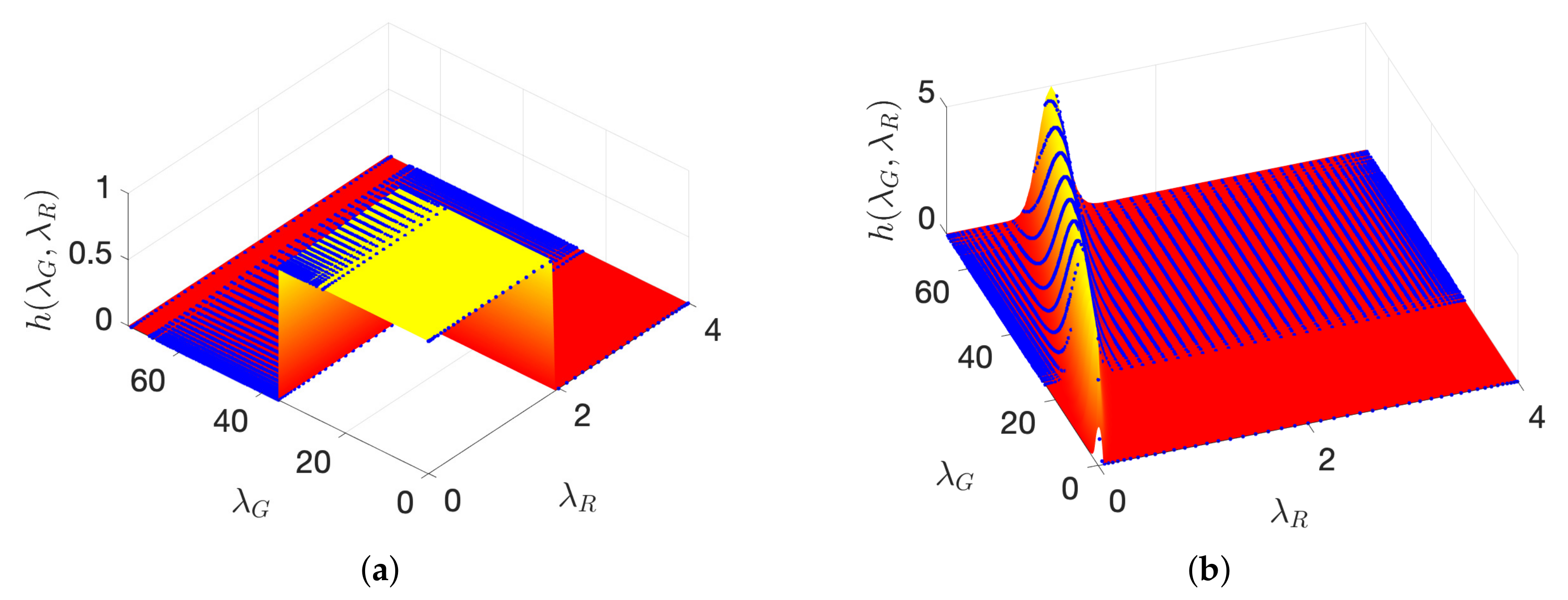
where has entries , and ∘ denotes the entry-wise product of two matrices. Figure 9 shows two examples of time-vertex filters: an ideal lowpass filter
and a wave filter
where is the largest eigenvalue of . The eigenvalues of range from 0 to 4 regardless of the size of T, so .
As a two-dimensional extension of spectral filtering, the time-vertex filtering decomposes the input signal into orthogonal components, where each component corresponds to an outer product of a graph Laplacian eigenvector and a DFT basis function. Then, the components are amplified or attenuated by the corresponding scalars . Finally, the scaled components are added together to obtain the filtered signal.
6.3. Spectrum-Adapted Approximation of Time-Vertex Filtering
Due to the high complexity of the spectral decomposition required to compute , approximation methods have been developed to accelerate joint time-vertex filtering, such as Chebyshev2D [64], ARMA2D [67], and the Fast Fourier Chebyshev algorithm [50].
As outlined in Algorithm 3, we can use the methods described in Section 3 to efficiently approximate the filtering of time-vertex signals. The overall complexity of our method is , where M is the number of nonzero entries in . The FFT of N discrete-time signals of length T takes . The loop computes T spectrum-adapted approximations to matrix functions with polynomials of degree K, and thus has a complexity of for sparse .
| Algorithm 3 Spectrum-adapted approximate time-vertex filtering. |
| Input weighted undirected graph G with N vertices, time-vertex signal , filter h |
| Output time-vertex filtered signal |
|
6.4. Numerical Experiments
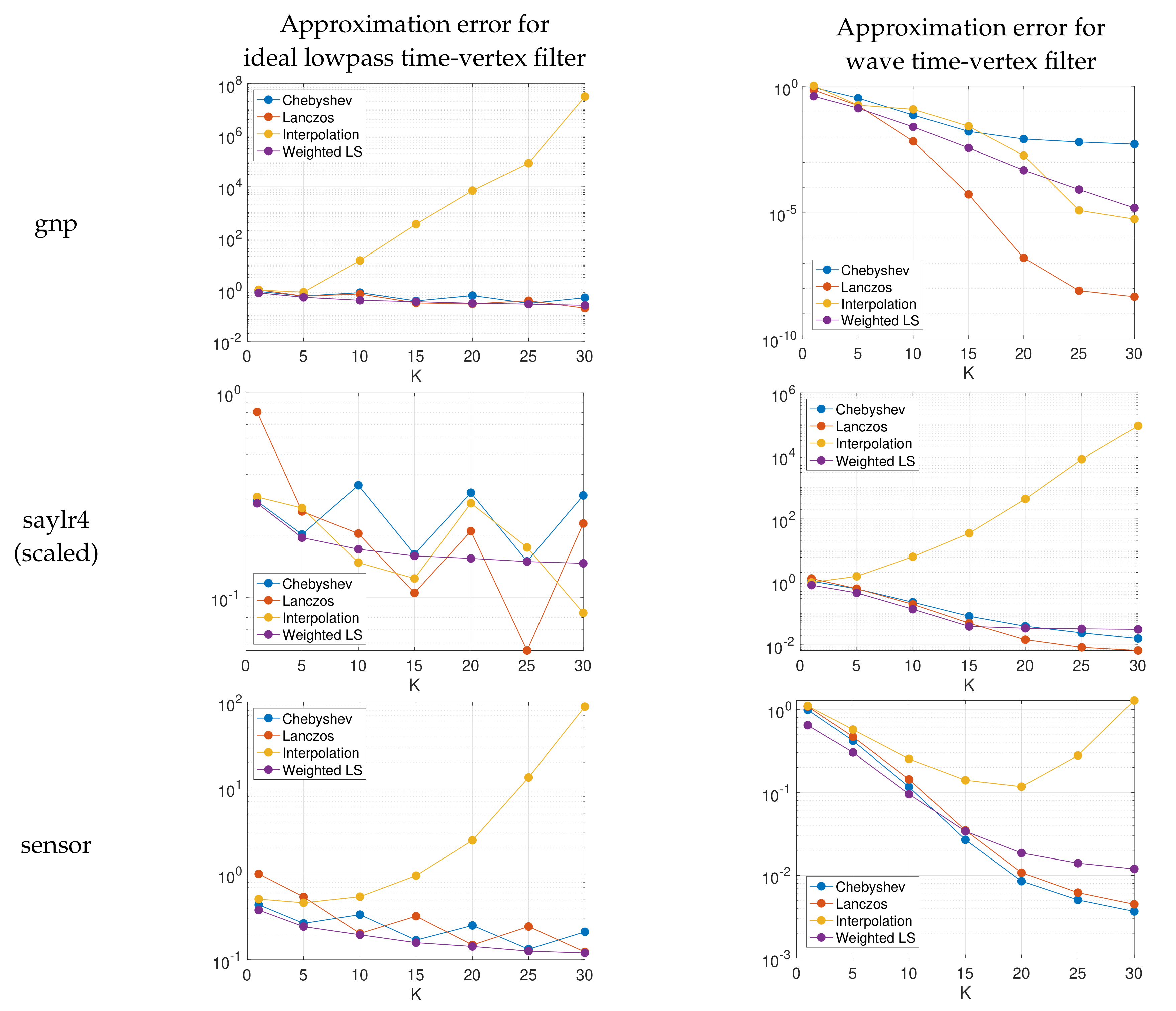
We consider the ideal lowpass filter (12) and the wave filter (13). We approximate for both filter functions, with observations, and for different graphs G: gnp (), saylr4 () and a random sensor network (), the cumulative spectral densities of which are shown in Figure 2. In each case, we choose , i.e., a constant vector in the joint spectral domain of and , in order to test the average performance of the approximation methods over different combinations of eigenvalue pairs. With polynomial approximation orders ranging from to 30, we follow the procedure described in Algorithm 3 to approximate . We estimate the cumulative spectral density functions with parameters , , and . We use in the spectrum-adapted polynomial regression/orthogonal polynomial expansion when finding the best polynomial approximation. We compare the proposed methods to the truncated Chebyshev expansion and the Lanczos method with the same polynomial order. For each method, we examine the convergence of relative errors in Frobenius norm as a function of K for graphs with various structures (and thus various distributions of Laplacian eigenvalues). The results are summarized in Figure 10. Similar to our observation in Figure 5, we see that the spectrum-adapted interpolation method performs well for lower polynomial orders , but tends to be unstable at higher polynomial orders.
6.5. Dynamic Mesh Denoising
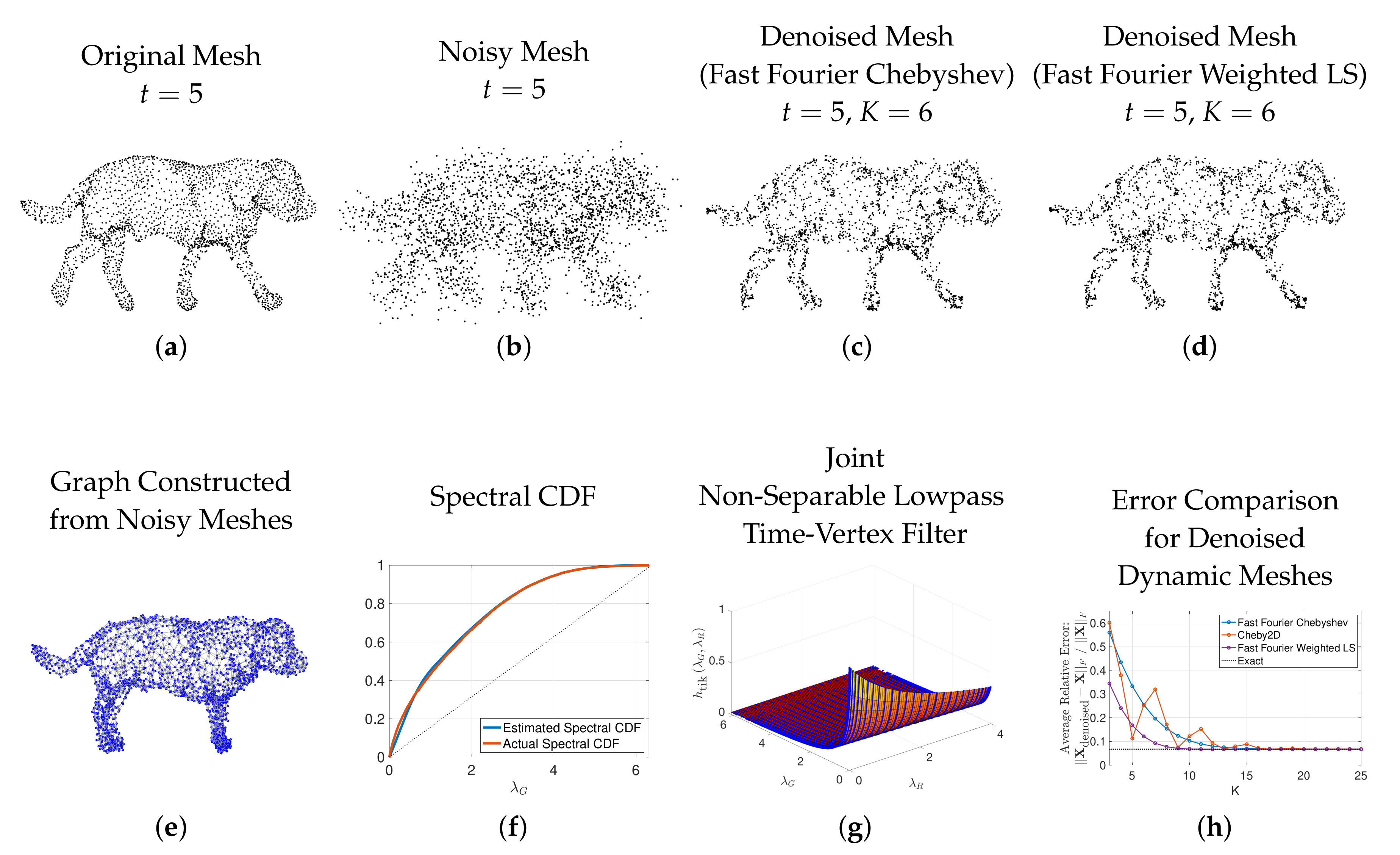
Finally, we replicate a dynamic mesh denoising example presented in [50] (Sec. VI.B). The original time-varying sequence of 3D meshes of a walking dog features meshes from time instances, each with points in 3D space (x-y-z coordinates). This sequence is denoted by the matrix . The original 3D mesh from time is shown in Figure 11a. The dynamic mesh sequence is corrupted by adding Gaussian noise (mean 0, standard deviation equal to ) to each mesh point coordinate. We denote the noisy 3D mesh sequence, one element of which is shown in Figure 11b, by . A single graph is created by subtracting the mean x, y, and z coordinates of each noisy mesh from that mesh, averaging the centered noisy mesh coordinates across all 59 time instances, and then building a 5-nearest neighbor graph on the average centered noisy mesh coordinates. The resulting graph and its spectral density function are shown in Figure 11e–f. The dynamic mesh sequence is denoised by solving the Tikhonov regularization problem [50] (Equation (30))
The optimization problem (14) has a closed-form solution
i.e., the joint time-vertex filtering operation defined in (11) is applied to each of the noisy x, y, and z coordinates, using the same joint non-separable lowpass filter , which is defined in the joint spectral domain as [50] (Equation (31))
We perform a grid search to find the values of the parameters and that minimize the relative error averaged over multiple realizations of the noise. In Figure 11g, we show the resulting filter with and on the joint spectrum of the graph shown in Figure 11e. The dashed black line in Figure 11h shows the relative error between the denoised sequence computed exactly in (15) and the original dynamic 3D mesh sequence, averaged over 20 realizations of the additive Gaussian noise. The other three curves in the same image show the average relative error when the computation in (15) is approximated by the fast Fourier Chebyshev method of [50], the Chebyshev2D method of [64], and the spectrum-adapted approximate time-vertex filtering (fast Fourier weighted least squares) of Algorithm 3, for different values of the polynomial degree K. All three approximations converge to the exact solution and corresponding error, but at low degrees (), the spectrum-adapted fast Fourier weighted least squares yields a better approximation. Figure 11c–d display examples of the denoised mesh at a single time () resulting from two of these approximations, with . The difference between the two is subtle, but can be seen, e.g., by scanning the top of the dog, where the mesh points form a slightly smoother surface.
7. Conclusions
We presented two novel spectrum-adapted polynomial methods for approximating for large sparse matrices: spectrum-adapted interpolation and spectrum-adapted weighted least squares/orthogonal polynomial expansion. These methods leverage an estimation of the cumulative spectral density of the matrix to build polynomials of a fixed order K that yield better approximations to f in the higher density regions of the matrix spectrum. In terms of approximation accuracy, numerical experiments showed that, relative to the state-of-the-art Lanczos and Chebysev polynomial approximation techniques, the proposed methods often yield more accurate approximations at lower polynomial orders; however, the proposed spectrum-adapted interpolation method is not very stable at higher degrees () due to overfitting. The proposed spectrum-adapted weighted least squares method performs particularly well in terms of accuracy for matrices with many distinct interior eigenvalues, whereas the Lanczos method, e.g., is often more accurate when K is higher and/or the matrix has many extreme eigenvalues. One potential extension would be to investigate a hybrid method that combines the Lanczos and spectrum-adapted weighted least squares approaches. We did not notice consistent trends regarding relative approximation accuracy with respect to the shape of the function f.
In terms of computational complexity, the cost of our methods, like Chebyshev polynomial approximation, is , where . For very large, sparse matrices, this complexity reduces to , where is an matrix. The Lanczos method, on the other hand, incurs an additional cost due to the orthogonalization step, making it more expensive for large enough K. Finally, the proposed spectrum-adapted methods, like the Chebyshev approximation, are amenable to efficient parallel and distributed computation via communication between neighboring nodes [33]. The inner products of the Lanczos method, on the other hand, may lead to additional communication expense or severe loss of efficiency in certain distributed computation environments (e.g., GPUs).
Author Contributions
Conceptualization, T.F., D.I.S., S.U., and Y.S.; data curation, T.F., D.I.S., and S.U.; formal analysis, T.F., D.I.S., and S.U.; funding acquisition, D.I.S.; investigation, T.F., D.I.S., and S.U.; methodology, T.F., D.I.S., S.U., and Y.S.; project administration, D.I.S.; software, T.F., D.I.S., and S.U.; supervision, D.I.S.; validation, T.F., D.I.S., and S.U.; visualization, T.F., D.I.S., and S.U.; writing—original draft, T.F., D.I.S., and S.U.; writing—review and editing, T.F., D.I.S., S.U., and Y.S. All authors have read and agreed to the published version of the manuscript.
Funding
This research received no external funding.
Acknowledgments
We thank the anonymous reviewers for their constructive comments on an earlier version of this article.
Conflicts of Interest
The authors declare no conflict of interest.
Reproducible Research
MATLAB code for all numerical experiments in this paper is available at http://www.macalester.edu/~dshuman1/publications.html. It leverages the open access GSPBox [57].
References
- Smola, A.J.; Kondor, R. Kernels and Regularization on Graphs. In Learning Theory and Kernel Machines; Lecture Notes in Computer Science; Schölkopf, B., Warmuth, M., Eds.; Springer: Berlin/Heidelberg, Germany, 2003; pp. 144–158. [Google Scholar]
- Belkin, M.; Matveeva, I.; Niyogi, P. Regularization and Semi-Supervised Learning on Large Graphs. In Learnning Theory; Lecture Notes in Computer Science; Springer: Berlin/Heidelberg, Germany, 2004; pp. 624–638. [Google Scholar]
- Zhou, D.; Bousquet, O.; Lal, T.N.; Weston, J.; Schölkopf, B. Learning with Local and Global Consistency; Advances Neural Information Processing Systems; Thrun, S., Saul, L., Schölkopf, B., Eds.; MIT Press: Cambridge, MA, USA, 2004; Volume 16, pp. 321–328. [Google Scholar]
- Shuman, D.I.; Narang, S.K.; Frossard, P.; Ortega, A.; Vandergheynst, P. The Emerging Field of Signal Processing on Graphs: Extending High-Dimensional Data Analysis to Networks and Other Irregular Domains. IEEE Signal Process. Mag. 2013, 30, 83–98. [Google Scholar] [CrossRef] [Green Version]
- Defferrard, M.; Bresson, X.; Vandergheynst, P. Convolutional Neural Networks on Graphs with Fast Localized Spectral Filtering; Advances Neural Information Processing Systems; MIT Press: Cambridge, MA, USA, 2016; pp. 3844–3852. [Google Scholar]
- Bronstein, M.M.; Bruna, J.; LeCun, Y.; Szlam, A.; Vandergheynst, P. Geometric Deep Learning: Going Beyond Euclidean Data. IEEE Signal Process. Mag. 2017, 34, 18–42. [Google Scholar] [CrossRef] [Green Version]
- Tremblay, N.; Puy, G.; Gribonval, R.; Vandergheynst, P. Compressive Spectral Clustering. Proc. Int. Conf. Mach. Learn. 2016, 48, 1002–1011. [Google Scholar]
- Orecchia, L.; Sachdeva, S.; Vishnoi, N.K. Approximating the Exponential, the Lanczos Method and an Õ(m)-Time Spectral Algorithm for Balanced Separator. Proc. ACM Symp. Theory Comput. 2012, 1141–1160. [Google Scholar] [CrossRef]
- Lin, L.; Saad, Y.; Yang, C. Approximating Spectral Densities of Large Matrices. SIAM Rev. 2016, 58, 34–65. [Google Scholar] [CrossRef]
- Ubaru, S.; Saad, Y. Fast Methods for Estimating the Numerical Rank of Large Matrices. Proc. Int. Conf. Mach. Learn. 2016, 48, 468–477. [Google Scholar]
- Ubaru, S.; Saad, Y.; Seghouane, A.K. Fast Estimation of Approximate Matrix Ranks Using Spectral Densities. Neural Comput. 2017, 29, 1317–1351. [Google Scholar] [CrossRef]
- Ubaru, S.; Chen, J.; Saad, Y. Fast Estimation of tr(f(A)) Via Stochastic Lanczos Quadrature. SIAM J. Matrix Anal. Appl. 2017, 38, 1075–1099. [Google Scholar] [CrossRef]
- Han, I.; Malioutov, D.; Avron, H.; Shin, J. Approximating Spectral Sums of Large-Scale Matrices Using Stochastic Chebyshev Approximations. SIAM J. Sci. Comput. 2017, 39, A1558–A1585. [Google Scholar] [CrossRef] [Green Version]
- Arora, S.; Kale, S. A Combinatorial, Primal-Dual Approach to Semidefinite Programs. Proc. ACM Symp. Theory Comput. 2007, 227–236. [Google Scholar] [CrossRef]
- Sachdeva, S.; Vishnoi, N.K. Faster Algorithms Via Approximation Theory. Found. Trends Theor. Comput. Sci. 2014, 9, 125–210. [Google Scholar] [CrossRef]
- Hochbruck, M.; Lubich, C.; Selhofer, H. Exponential Integrators for Large Systems of Differential Equations. SIAM J. Sci. Comput. 1998, 19, 1552–1574. [Google Scholar] [CrossRef] [Green Version]
- Friesner, R.A.; Tuckerman, L.; Dornblaser, B.; Russo, T.V. A Method for Exponential Propagation of Large Systems of Stiff Nonlinear Differential Equations. J. Sci. Comput. 1989, 4, 327–354. [Google Scholar] [CrossRef]
- Gallopoulos, E.; Saad, Y. Efficient Solution of Parabolic Equations by Krylov Approximation Methods. SIAM J. Sci. Stat. Comput. 1992, 13, 1236–1264. [Google Scholar] [CrossRef] [Green Version]
- Higham, N.J. Functions of Matrices; SIAM: Philadelphia, PA, USA, 2008. [Google Scholar]
- Davies, P.I.; Higham, N.J. Computing f(A)b for Matrix Functions f. In QCD and Numerical Analysis III; Springer: Berlin/Heidelberg, Germany, 2005; pp. 15–24. [Google Scholar]
- Frommer, A.; Simoncini, V. Matrix Functions. In Model Order Reduction: Theory, Research Aspects and Applications; Springer: Berlin/Heidelberg, Germany, 2008; pp. 275–303. [Google Scholar]
- Moler, C.; Van Loan, C. Nineteen Dubious Ways to Compute the Exponential of a Matrix, Twenty-Five Years Later. SIAM Rev. 2003, 45, 3–49. [Google Scholar] [CrossRef]
- Druskin, V.L.; Knizhnerman, L.A. Two Polynomial Methods of Calculating Functions of Symmetric Matrices. USSR Comput. Maths. Math. Phys. 1989, 29, 112–121. [Google Scholar] [CrossRef]
- Saad, Y. Filtered Conjugate Residual-Type Algorithms with Applications. SIAM J. Matrix Anal. Appl. 2006, 28, 845–870. [Google Scholar] [CrossRef] [Green Version]
- Chen, J.; Anitescu, M.; Saad, Y. Computing f(A)b Via Least Squares Polynomial Approximations. SIAM J. Sci. Comp. 2011, 33, 195–222. [Google Scholar] [CrossRef] [Green Version]
- Druskin, V.; Knizhnerman, L. Extended Krylov Subspaces: Approximation of the Matrix Square Root and Related Functions. SIAM J. Matrix Anal. Appl. 1998, 19, 755–771. [Google Scholar] [CrossRef]
- Eiermann, M.; Ernst, O.G. A Restarted Krylov Subspace Method for the Evaluation of Matrix Functions. SIAM J. Numer. Anal. 2006, 44, 2481–2504. [Google Scholar] [CrossRef] [Green Version]
- Afanasjew, M.; Eiermann, M.; Ernst, O.G.; Güttel, S. Implementation of a Restarted Krylov Subspace Method for the Evaluation of Matrix Functions. Lin. Alg. Appl. 2008, 429, 2293–2314. [Google Scholar] [CrossRef]
- Frommer, A.; Lund, K.; Schweitzer, M.; Szyld, D.B. The Radau-Lanczos Method for Matrix Functions. SIAM J. Matrix Anal. Appl. 2017, 38, 710–732. [Google Scholar] [CrossRef] [Green Version]
- Golub, G.H.; Van Loan, C.F. Matrix Computations; Johns Hopkins University Press: Baltimore, MD, USA, 2013. [Google Scholar]
- Mason, J.C.; Handscomb, D.C. Chebyshev Polynomials; Chapman and Hall: London, UK, 2003. [Google Scholar]
- Trefethen, L.N. Approximation Theory and Approximation Practice; SIAM: Philadelphia, PA, USA, 2013. [Google Scholar]
- Shuman, D.I.; Vandergheynst, P.; Kressner, D.; Frossard, P. Distributed Signal Processing via Chebyshev Polynomial Approximation. IEEE Trans. Signal Inf. Process. Netw. 2018, 4, 736–751. [Google Scholar] [CrossRef] [Green Version]
- Hammond, D.K.; Vandergheynst, P.; Gribonval, R. Wavelets on Graphs Via Spectral Graph Theory. Appl. Comput. Harmon. Anal. 2011, 30, 129–150. [Google Scholar] [CrossRef] [Green Version]
- Segarra, S.; Marques, A.G.; Ribeiro, A. Optimal Graph-Filter Design and Applications to Distributed Linear Network Operators. IEEE Trans. Signal Process. 2017, 65, 4117–4131. [Google Scholar] [CrossRef]
- Van Mieghem, P. Graph Spectra for Complex Networks; Cambridge University Press: Cambridge, UK, 2011. [Google Scholar]
- Tao, T. Topics in Random Matrix Theory; American Mathematical Society: Providence, RI, USA, 2012. [Google Scholar]
- Silver, R.N.; Röder, H. Densities of States of Mega-Dimensional Hamiltonian Matrices. Int. J. Mod. Phys. C 1994, 5, 735–753. [Google Scholar] [CrossRef]
- Silver, R.N.; Röder, H.; Voter, A.F.; Kress, J.D. Kernel Polynomial Approximations for Densities of States and Spectral Functions. J. Comput. Phys. 1996, 124, 115–130. [Google Scholar] [CrossRef]
- Wang, L.W. Calculating the Density of States and Optical-Absorption Spectra of Large Quantum Systems by the Plane-Wave Moments Method. Phy. Rev. B 1994, 49, 10154. [Google Scholar] [CrossRef]
- Li, S.; Jin, Y.; Shuman, D.I. Scalable M-channel critically sampled filter banks for graph signals. IEEE Trans. Signal Process. 2019, 67, 3954–3969. [Google Scholar] [CrossRef] [Green Version]
- Girard, D. Un Algorithme Simple et Rapide Pour la Validation Croisée Généralisée sur des Problèmes de Grande Taille; Technical Report; Université Grenoble Alpes: St Martin d’Hères, France, 1987. [Google Scholar]
- Girard, A. A fast ’Monte-Carlo cross-validation’procedure for large least squares problems with noisy data. Numer. Math. 1989, 56, 1–23. [Google Scholar] [CrossRef]
- Di Napoli, E.; Polizzi, E.; Saad, Y. Efficient Estimation of Eigenvalue Counts in an Interval. Numer. Linear Algebra Appl. 2016, 23, 674–692. [Google Scholar] [CrossRef] [Green Version]
- Puy, G.; Pérez, P. Structured Sampling and Fast Reconstruction of Smooth Graph Signals. Inf. Inference A J. IMA 2018, 7, 657–688. [Google Scholar] [CrossRef] [Green Version]
- Shuman, D.I.; Wiesmeyr, C.; Holighaus, N.; Vandergheynst, P. Spectrum-Adapted Tight Graph Wavelet and Vertex-Frequency Frames. IEEE Trans. Signal Process. 2015, 63, 4223–4235. [Google Scholar] [CrossRef] [Green Version]
- Fritsch, F.N.; Carlson, R.E. Monotone Piecewise Cubic Interpolation. SIAM J. Numer. Anal. 1980, 17, 238–246. [Google Scholar] [CrossRef]
- Gleich, D. The MatlabBGL Matlab Library. Available online: http://www.cs.purdue.edu/homes/dgleich/packages/matlab_bgl/index.html (accessed on 11 November 2020).
- Stanford University Computer Graphics Laboratory. The Stanford 3D Scanning Repository. Available online: http://graphics.stanford.edu/data/3Dscanrep/ (accessed on 11 November 2020).
- Grassi, F.; Loukas, A.; Perraudin, N.; Ricaud, B. A Time-Vertex Signal Processing Framework: Scalable Processing and Meaningful Representations for Time-Series on Graphs. IEEE Trans. Signal Process. 2018, 66, 817–829. [Google Scholar] [CrossRef] [Green Version]
- Davis, T.A.; Hu, Y. The University of Florida Sparse Matrix Collection. ACM Trans. Math. Softw. 2011, 38, 1:1–1:25. [Google Scholar] [CrossRef]
- Forsythe, G.E. Generation and Use of Orthogonal Polynomials for Data-Fitting with a Digital Computer. J. SIAM 1957, 5, 74–88. [Google Scholar] [CrossRef]
- Gautschi, W. Orthogonal Polynomials: Computation and Approximation; Oxford University Press: Oxford, UK, 2004. [Google Scholar]
- Gragg, W.B.; Harrod, W.J. The Numerically Stable Reconstruction of Jacobi Matrices from Spectral Data. Numer. Math. 1984, 44, 317–335. [Google Scholar] [CrossRef]
- Saad, Y. Analysis of Some Krylov Subspace Approximations to the Matrix Exponential Operator. SIAM J. Numer. Anal. 1992, 29, 209–228. [Google Scholar] [CrossRef]
- Golub, G.H.; Meurant, G. Matrices, Moments and Quadrature with Applications; Princeton University Press: Princeton, NJ, USA, 2010. [Google Scholar]
- Perraudin, N.; Paratte, J.; Shuman, D.I.; Kalofolias, V.; Vandergheynst, P.; Hammond, D.K. GSPBOX: A Toolbox for Signal Processing on Graphs. arXiv 2014, arXiv:1408.5781. Available online: https://epfl-lts2.github.io/gspbox-html/ (accessed on 11 November 2020).
- Shuman, D.I. Localized Spectral Graph Filter Frames: A Unifying Framework, Survey of Design Considerations, and Numerical Comparison. IEEE Signal Process. Mag. 2020, 37, 43–63. [Google Scholar] [CrossRef]
- Göbel, F.; Blanchard, G.; von Luxburg, U. Construction of tight frames on graphs and application to denoising. In Handbook of Big Data Analytics; Springer: Berlin/Heidelberg, Germany, 2018; pp. 503–522. [Google Scholar]
- de Loynes, B.; Navarro, F.; Olivier, B. Data-Driven Thresholding in Denoising with Spectral Graph Wavelet Transform. arXiv 2019, arXiv:1906.01882. [Google Scholar]
- Puy, G.; Tremblay, N.; Gribonval, R.; Vandergheynst, P. Random sampling of bandlimited signals on graphs. Appl. Comput. Harmon. Anal. 2018, 44, 446–475. [Google Scholar] [CrossRef] [Green Version]
- Benzi, M.; Boito, P. Quadrature Rule-Based Bounds for Functions of Adjacency Matrices. Lin. Alg. Appl. 2010, 433, 637–652. [Google Scholar] [CrossRef] [Green Version]
- Bekas, C.; Kokiopoulou, E.; Saad, Y. An Estimator for the Diagonal of a Matrix. Appl. Numer. Math. 2007, 57, 1214–1229. [Google Scholar] [CrossRef] [Green Version]
- Loukas, A.; Foucard, D. Frequency Analysis of Time-Varying Graph Signals. In Proceedings of the 2016 IEEE Global Conference on Signal and Information Processing (GlobalSIP), Washington, DC, USA, 7–9 December 2016; pp. 346–350. [Google Scholar]
- Perraudin, N.; Loukas, A.; Grassi, F.; Vandergheynst, P. Towards Stationary Time-Vertex Signal Processing. In Proceedings of the 2017 IEEE International Conference on Acoustics, Speech and Signal Processing (ICASSP), New Orleans, LA, USA, 5–9 March 2017; pp. 3914–3918. [Google Scholar]
- Grady, L.J.; Polimeni, J.R. Discrete Calculus; Springer: Berlin/Heidelberg, Germany, 2010. [Google Scholar]
- Isufi, E.; Loukas, A.; Simonetto, A.; Leus, G. Separable Autoregressive Moving Average Graph-Temporal Filters. In Proceedings of the 2016 24th European Signal Processing Conference (EUSIPCO), Budapest, Hungary, 29 August–2 September 2016; pp. 200–204. [Google Scholar]
Figure 1.
Degree 5 polynomial approximations of the function of the graph Laplacian of a random Erdös–Renyi graph with 500 vertices and edge probability 0.2. The discrete least squares approximation incurs larger errors in the lower end of the spectrum. However, since the eigenvalues are concentrated at the upper end of the spectrum, it yields a lower approximation error .

Figure 2.
Estimated and actual cumulative spectral density functions for eight real, symmetric matrices A. We estimate the eigenvalue counts for linearly spaced points on via (6), with degree polynomials and random vectors .
Figure 2.
Estimated and actual cumulative spectral density functions for eight real, symmetric matrices A. We estimate the eigenvalue counts for linearly spaced points on via (6), with degree polynomials and random vectors .

Figure 3.
Construction of six interpolation points for the same graph Laplacian matrix described in Figure 1. The interpolation points on the horizontal axis are computed by applying the inverse of the estimated cumulative spectral density function to the initial Chebyshev points on the vertical axis.

Figure 4.
Comparison of (top) the first six discrete orthogonal polynomials defined in (8), adapted to the estimated cumulative spectral density of the random Erdös–Renyi graph from Figure 1, Figure 2 and Figure 3, to (bottom) the first six standard shifted Chebyshev polynomials with degree to 5. In the region of high spectral density, shown in the zoomed boxes on the right, the discrete orthogonal polynomials feature more oscillation while maintaining small amplitudes, enabling better approximation of smooth functions in this region.

Figure 5.
Approximations of with and equal to (first two columns) and lowpass, bandpass, and highpass spectral graph filters (last three columns, respectively).
Figure 5.
Approximations of with and equal to (first two columns) and lowpass, bandpass, and highpass spectral graph filters (last three columns, respectively).


Figure 6.
Spectral graph filter bank examples. (a) A set of five uniform translates of an itersine kernel [46,57]. (b) A set of four log-warped translates (also called octave-band or wavelet filters) [46]. We plot both sets of spectral graph filters on the spectrum of the Stanford bunny graph with vertices; however, the design only depends on the spectral range , so the filters will look the same (except stretched) for all graphs considered, e.g., in Figure 5.

Figure 7.
Estimation of the norms of the atoms of spectral graph wavelet dictionaries. (a) Exact atom norms, , colored by the indices of the generating filters (shown in Figure 6), each of which is localized to every vertex on the bunny graph. (b) Comparison of the estimated norms, , to the corresponding exact norms (shown in black). The atoms are sorted in descending order of exact norm to aid visual comparison. (c) The ratios of the estimated norms to the exact atom norms. (d–f) The mean relative errors across all atoms for dictionaries generated by the same set of filters on three different graphs, with varying polynomial approximation methods, polynomial degrees K, and numbers of random vectors J.

Figure 8.
A time-vertex signal defined on a sensor graph G with vertices and observations, visualized on a multilayer graph structure. Each layer is a copy of G observed at one time point.
Figure 8.
A time-vertex signal defined on a sensor graph G with vertices and observations, visualized on a multilayer graph structure. Each layer is a copy of G observed at one time point.

Figure 9.
Two time-vertex filters defined for a random Erdös–Renyi graph with 500 vertices and edge probability 0.2. (a) An ideal lowpass filter; (b) a wave filter. The blue dots correspond to the positions of eigenvalue pairs.
Figure 9.
Two time-vertex filters defined for a random Erdös–Renyi graph with 500 vertices and edge probability 0.2. (a) An ideal lowpass filter; (b) a wave filter. The blue dots correspond to the positions of eigenvalue pairs.


Figure 11.
Denoising of a time-varying sequence of 3D meshes of a walking dog. Top row: one element each of the dynamic sequences of (a) original, (b) noisy, and (c,d) denoised (using two different approximation methods) meshes. Bottom row: (e,f) a 5-nearest neighbor graph (and its spectral CDF) constructed from the entire sequence of noisy meshes, which is used to denoise the meshes at all times instances; (g) the joint time-vertex lowpass filter (16); and (h) the average relative errors between the original sequence of meshes and the denoised versions attained by exactly or approximately computing (15) with different polynomial approximation methods, for a range of polynomial degrees.

Publisher’s Note: MDPI stays neutral with regard to jurisdictional claims in published maps and institutional affiliations. |
© 2020 by the authors. Licensee MDPI, Basel, Switzerland. This article is an open access article distributed under the terms and conditions of the Creative Commons Attribution (CC BY) license (http://creativecommons.org/licenses/by/4.0/).
Share and Cite
MDPI and ACS Style
Fan, T.; Shuman, D.I.; Ubaru, S.; Saad, Y. Spectrum-Adapted Polynomial Approximation for Matrix Functions with Applications in Graph Signal Processing. Algorithms 2020, 13, 295. https://0-doi-org.brum.beds.ac.uk/10.3390/a13110295
AMA Style
Fan T, Shuman DI, Ubaru S, Saad Y. Spectrum-Adapted Polynomial Approximation for Matrix Functions with Applications in Graph Signal Processing. Algorithms. 2020; 13(11):295. https://0-doi-org.brum.beds.ac.uk/10.3390/a13110295
Chicago/Turabian StyleFan, Tiffany, David I. Shuman, Shashanka Ubaru, and Yousef Saad. 2020. "Spectrum-Adapted Polynomial Approximation for Matrix Functions with Applications in Graph Signal Processing" Algorithms 13, no. 11: 295. https://0-doi-org.brum.beds.ac.uk/10.3390/a13110295
Note that from the first issue of 2016, this journal uses article numbers instead of page numbers. See further details here.