A Dynamic Route-Planning System Based on Industry 4.0 Technology


School of Management Technology, Sirindhorn International Institute of Technology, Thammasat University, Pathum Thani 12120, Thailand
*
Author to whom correspondence should be addressed.
Algorithms 2020, 13(12), 308; https://0-doi-org.brum.beds.ac.uk/10.3390/a13120308
Submission received: 28 October 2020
/
Revised: 17 November 2020
/
Accepted: 23 November 2020
/
Published: 25 November 2020
(This article belongs to the Special Issue Algorithms for Shortest Paths in Dynamic and Evolving Networks)
Abstract
:Due to the availability of Industry 4.0 technology, the application of big data analytics to automated systems is possible. The distribution of products between warehouses or within a warehouse is an area that can benefit from automation based on Industry 4.0 technology. In this paper, the focus was on developing a dynamic route-planning system for automated guided vehicles within a warehouse. A dynamic routing problem with real-time obstacles was considered in this research. A key problem in this research area is the lack of a real-time route-planning algorithm that is suitable for the implementation on automated guided vehicles with limited computing resources. An optimization model, as well as machine learning methodologies for determining an operational route for the problem, is proposed. An internal layout of the warehouse of a large consumer product distributor was used to test the performance of the methodologies. A simulation environment based on Gazebo was developed and used for testing the implementation of the route-planning system. Computational results show that the proposed machine learning methodologies were able to generate routes with testing accuracy of up to 98% for a practical internal layout of a warehouse with 18 storage racks and 67 path segments. Managerial insights into how the machine learning configuration affects the prediction accuracy are also provided.
1. Introduction
Currently, Industry 4.0 technology has the potential to impact the operations of many industries. As shown in Figure 1, big data and analytics and autonomous robots are the two main components of Industry 4.0 technology [1]. Autonomous robots are increasingly used to automate routine tasks in many industrial applications and tasks in special areas that are harmful to operators. Artificial intelligence (AI)-based automation is adaptive and has many practical applications in different industries. The transportation industry is one of the areas that has potential for the application of AI-based automation, especially in supply chains, where there are large amounts of transactional data at every stage. As such, the processes involved can receive benefit from AI and robotics automation. The advancement of AI and robotics technologies brings about new opportunities for improving the operations across a supply chain. With AI and robotics automation, organizations can collect and perform data analysis autonomously, which improves supply chain responsiveness. New breakthroughs in AI, robotics, and automation can accelerate material development, the flow of products, material handling, and quality control in an integrated environment [2]. The efficiency of operations within a warehouse can be improved with the application of AI-based automation due to the high rates of movement of products. One of the famous warehouse robot systems is the Kiva system implemented at Amazon. The system was used to improve the efficiency of warehouse operations [3].
The focus of this research was on developing an AI-based automation methodology for controlling the movement of automated vehicles within a warehouse. In a typical operation within a warehouse, the amount of daily product movement is huge, and, in general, the routes are determined on the basis of the experience of drivers. Dynamic obstacles can obstruct the movement through some path segments within a warehouse and could affect the routes that can be used by the drivers. A route-planning process with the consideration of dynamic obstacles is complex and cannot rely only on human experience. In this research, methodologies for determining routes that consider real-time obstacles are presented. The methodologies include an optimization model for routing decision, an A-star heuristic method, and machine learning models based on an artificial neural network (ANN). The novelty of this research can be summarized as follows:
- This research presents a route-planning methodology based on an ANN. The ANN can be implemented on automated guided vehicles (AGVs) with limited computing resources. Once an ANN is trained, it can generate a route with minimal computational effort and runtime (less than a second).
- The considered route-planning problem is based on a practical warehouse environment that considers real-time obstacles.
- A route-planning system that collects the data for training an ANN and generates routes on the basis of real-time positions of obstacles is introduced.
- The proposed methodology is adaptive and scalable. It can be applied to other routing problems with different requirements. Heuristic methods can be used for generating routes for large-scale problems.
- This research presents managerial insights into how the configuration of an ANN affects the accuracy, and how the best configuration can be chosen.
The organization of this paper is as follows: Section 2 presents a literature review related to motion planning and route planning. A mathematical model for routing decisions and an A-star heuristic are described in Section 3. An ANN model for dynamic route planning is presented in Section 4. The transportation environment used in this research is presented in Section 5. A dynamic routing system and computational results with managerial insights are presented in Section 6. The conclusions and possible future research are discussed in Section 7.
2. Literature Review
The planning of autonomous movement of a robot is related to two main areas, motion planning and route (or path) planning. A literature review of key articles and the research gap are provided in this section.
2.1. Motion Planning
When applying motion planning to the autonomous movement of a robot, the goal is to determine a sequence of motion that moves the robot from an origin to a destination. In general, a motion planning has obstacle collision avoidance capability, using available data from different equipped sensors to navigate the robot by controlling the speed and direction of movement. an A-star algorithm has been applied to many motion planning problems and is considered one of the most popular algorithms.
Liu and Gong [4] applied many variations of the A-star algorithm for path planning for a rescue robot operation. They presented many variations of the A-star algorithm according to the complexity of the rescue environment, as well as the precision of the sensors. Because of the noise from the signals detected by the robot, approximated information of the robot’s orientation is required. El Halawany et al. [5] stated that A-star is the best general algorithm for searching for the optimal path. Path planning is used in many types of applications, especially in artificial intelligence-related areas. Contreras-González et al. [6] developed an ANN to predict the location of an AGV by using operational data containing the accuracy from the model and the actual location of the AGV. The proposed ANN model could generate a smooth and accurate point-to-point travel plan in field testing without a controlled environment. Zhang et al. [7] proposed an enhanced A-star algorithm for guiding an automated guided vehicle (AGV). The proposed method could generate efficient paths that reduce superfluous inflection points and redundant nodes. Gochev et al. [8] proposed an integration of a collision avoidance method and the A-star algorithm in an environment with different agents for an AGV system. In the experiment, the AGVs had to follow different assigned paths without colliding with the obstacles. Mohan and Ignatious [9] studied an application of a mobile robot in a warehouse environment with the monitoring of battery health. An enhanced A-star algorithm was used to generate the paths for robots. Kurdi et al. [10] developed an intelligent controller for path planning using an ANN. The authors constructed collision-free paths for moving robots among obstacles on the basis of multiple inputs from different resources. Zhang et al. [11] proposed an ANN model for path control of an AGV that considers the line-of-sight during movement in adverse conditions. The ANN model was created for learning the proposed guidance law in order to control the effects of wind-induced sideslips. Flórez et al. [12] developed a control methodology for an AGV. A hybrid kinematic controller was developed on the basis of a combination of an evolved ANN and a genetic algorithm. The controller was used to control car kinematics to avoid obstacles. From the test results, the vehicle reached a certain level of autonomy, according to a controller that took into account the kinematics and dynamics of the system. A new suggested method that combined A-star algorithm and motion planning, and that could find a global path, track the path, and avoid collisions in a dynamic environment, as well as in a static one, was introduced by Zhong et al. [13]. For real-time obstacles, path planning with A-star generated a global path that kept distance from the obstacles; the path was tracked with a window adaptive approach that helped the robot track the entire path smoothly and reach the final goal without collisions.
2.2. Route Planning
Bhadoria and Singh [14] showed that algorithms such as Dijkstra and A-star can be applied for both path planning and routing decisions. Many scenarios were created on the basis of an unstructured and unpredictable environment, where the robots were forced to face new situations in which decision-making was quite difficult. Zhang and Zhao [15] considered an integrated framework for combining A-star and a Dijkstra algorithm. The proposed algorithm was used to guide a mobile robot along the path between an origin and a provided destination with the ability to avoid collisions with obstacles. Kusuma and Machbub [16] implemented an A-star algorithm for planning the movement of a humanoid robot. The proposed algorithm had the ability to find a new route if the destination was modified or if the robot failed to follow the assigned path. Ruiz et al. [17] considered an open vehicle routing problem with the capacity limitation and distance constraints. A biased random-key genetic algorithm designed to solve the problem was benchmarked with three datasets to demonstrate the efficiency of the proposed algorithm. Salavati-Khoshghalb et al. [18] investigated a vehicle routing problem (VRP) that considered uncertainty in demand under a restocking policy. An integer L-shaped algorithm and various lower bound schemes were developed to determine the solutions for problems with up to 60 customers and four vehicles. Zhang et al. [19] studied an ant colony optimization algorithm for a multi-objective vehicle routing problem with flexible time windows. The model aimed to simultaneously minimize the total distribution costs and maximize the overall customer satisfaction. Sung et al. [20] developed a neural network that could be used to determine a collision-free path in a large-scale dynamic environment generated from a dataset that was extracted from a Bellman–Ford algorithm and a quadratic program. The dataset from the Bellman–Ford algorithm showed better reliability for training the neural network due to the appropriateness of this algorithm in a discretized space. Pasha et al. [21] formulated a mixed-integer linear programming model for an open capacitated VRP with soft time windows. An optimization model and four metaheuristic algorithms were developed to solve the problem. The results showed that the evolutionary algorithm provided good-quality solutions for both the small-scale and the large-scale problems with practical runtime. Trachanatzi et al. [22] addressed an environmental prize-collecting vehicle routing problem. A firefly algorithm based on coordinates (FAC) was designed to solve the model. The proposed algorithm was performed and tested with many instances from previous studies to demonstrate the promising performance of the FAC. A summary of the methods used in key related articles is shown in Table 1. According to the literature review, route-planning and path problems for AGV are active research areas related to Industry 4.0 technology. None of the research addressed an adaptive solution methodology for a route-planning problem within a warehouse that considers real-time obstacles. The present research focused on developing a solution methodology using ANN for a route-planning problem with real-time obstacles. A dynamic route-planning system is also proposed. The main contribution of this research is the development of an efficient route-planning methodology using a machine learning model that can be implemented on AGVs with limited computing resources. An ANN model that can be used to determine the parameters that specify the relationship between the input and output of a dynamic route-planning problem is introduced. This can then be applied to predict the route on the basis of different scenarios of input data.
3. Models and Algorithms for Route Planning
To determine a solution for a route-planning problem, both an optimization model and a heuristic algorithm were used. In this section, a shortest-path model is introduced and used as a benchmark for testing the quality of solutions from other methods. A heuristic method based on an A-star algorithm is presented next.
3.1. An Optimization Model for Route Planning
A shortest-path model is used for comparing the results from other methods. The model is summarized as follows [23]: given a directed graph G = (V, A), where V and A represent a set of nodes and a set of arcs of the graph. The shortest-path problem determines a path with the minimum distance between two nodes, s (source or starting) and t (target or destination). The cardinality of V and A are represented by parameters n and m, respectively. A path is a sequence of nodes v1, …, vk, and it is considered to be elementary if no node is visited more than once.
Let δ+(i) and δ−(i) represent sets of arcs leaving and entering node i ∈ V, and let A(S) be a set of arcs with both ends in S ⊆ V.
Indices, parameters, and decision variables are presented as follows:
- Indices
- i, j, and k: indices representing nodes in G
- A: a set of arcs from G
- Parameters
- cij: distance from node i to j, (i, j) ∈ A
- Z: the total distance
- Decision variables
- xij is equals to 1 if (i,j) is chosen and 0 otherwise.
The objective function and constraints for the shortest-path problem are presented next.
xij ≥ 0 for (i,j) ∈ A, x ∈ Z|A|.
The objective function is represented by Equation (1), where the total distance is minimized. Equations (2) and (4) represent the net flow at nodes s and t, where the net flow at node s is 1, and the net flow at node t is −1. The flow conservation constraints for nodes other that s and t are represented by Equation (3). When applying a shortest-path model for determining a solution for a dynamic route-planning problem, the distance (cij) associated with each path segment (defined by (i,j)) that contains an obstacle and cannot be used is set to a large value that is based on the size of the transportation area. If there exists a feasible solution, the segments with large cost values are not selected in the optimal solution.
3.2. A Heuristic Algorithm for Path Planning (A-Star Algorithm)
In this study, an A-star algorithm was used to identify a path that avoids obstacles on any path segment. The algorithm can be described as follows:
During the path search of an A-star algorithm, an “OPENED” list and a “CLOSED” list are used to keep track information during the search. The “OPENED” list stores the paths that will be explored. The “CLOSED” list contains all explored paths. Let h(n) represent the cost from an origin to the current node (n) and let g(n) represent the cost to get from the current node (n) to a destination node. The total cost, f(n), is calculated for each successor node that includes both h(n) and g(n). The procedure consist of seven steps [24]:
- The start node is removed from the “OPENED” list. The cost function f(n) is calculated; note that h(n) = 0 and g(n) are calculated on the basis of the distance between the start position and the destination (f(n) = g(n)).
- A node with the smallest cost function is removed from the “OPENED” list and inserted into the “CLOSED” list. The node is set as node n (break ties arbitrarily, if two or more nodes have the same cost function). If one of the nodes is the destination node, then the destination node is selected.
- If n is the destination node, the algorithm is terminated; otherwise, it continues.
- The cost function for each successor of n that is not on the “CLOSED” list is computed.
- Each successor not on the “OPENED” list or CLOSED list is associated with the calculated cost and put on the “OPENED” list.
- Any successor already on the “OPENED” list is associated with the minimum cost (min(new(f(n)), old(f(n)))).
- Return to step 2.
4. Results
Initially, the models in Section 3 were used to determine the solutions for a route-planning problem. For an optimization model, the solutions can be determined by using a mathematical solver such as CPLEX; for a heuristic method based on the A-star algorithm, the solution is generated by an installed executable module. This requires high-performance hardware with high computational capacity, where the computational runtime varies according to the dimension of input data instance. In order to utilize knowledge gained from previously solved data instances, the input data instances, as well as the generated routes, were collected and used to build an ANN model that can identify an optimal route. This process requires less computational effort and is suitable to implement on a mobile robot with limited computing capability. Having to execute a heuristic algorithm or a mathematical solver every time to generate a route is inefficient. This is because, once an ANN is trained, it can generate a route with minimal computational effort and runtime (less than a second). An ANN training process requires a server equipped with MATLAB, and it can be executed on a weekly basis or when the ANN needs an update.
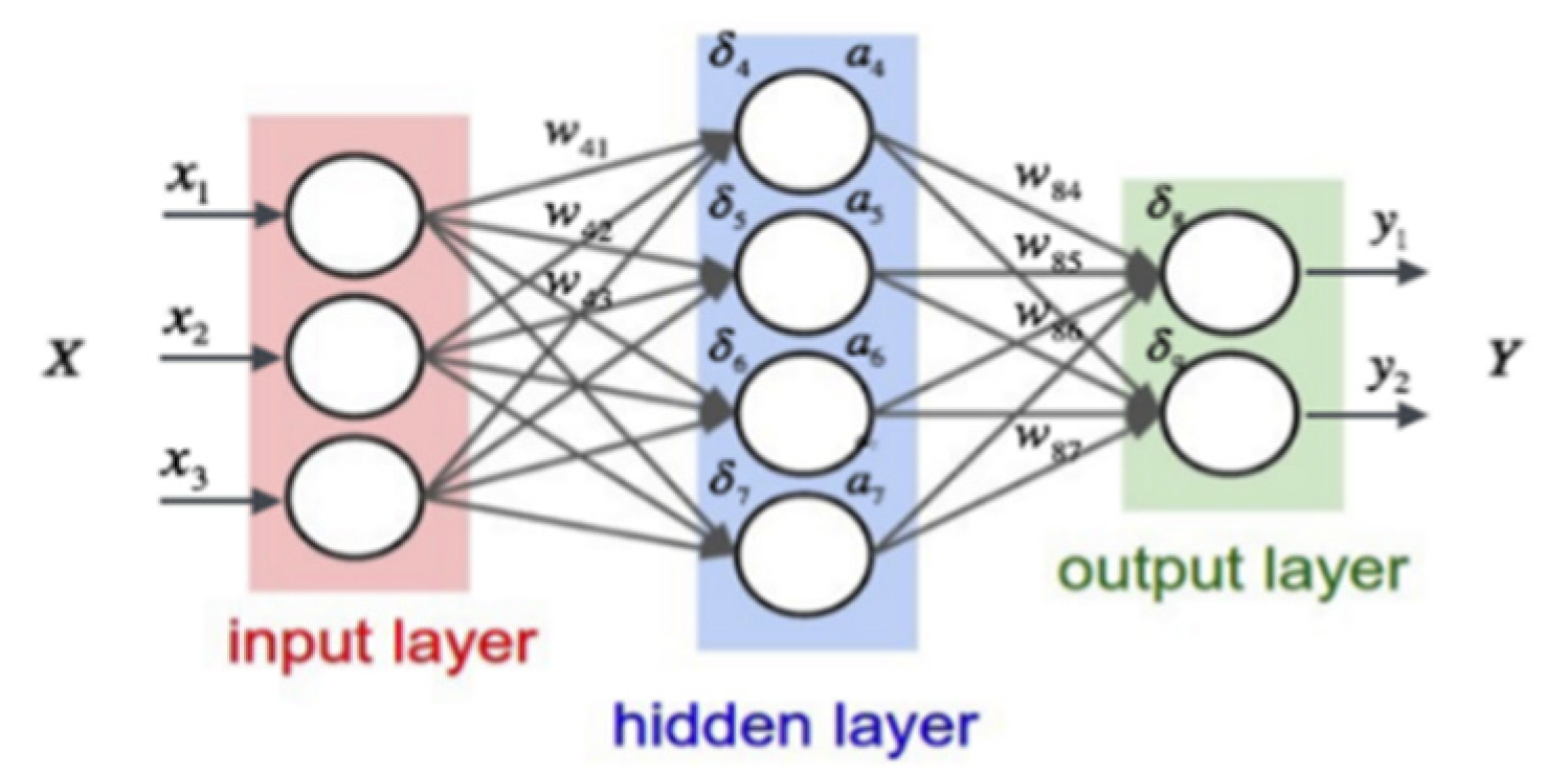
The structure of a feed-forward ANN model for a dynamic route-planning problem is shown in Figure 2. The inputs and outputs of the ANN were defined on the basis of a layout of the simulated transportation area, which was defined by a two-dimensional grid map. An example of a grid map is shown in Figure 3.
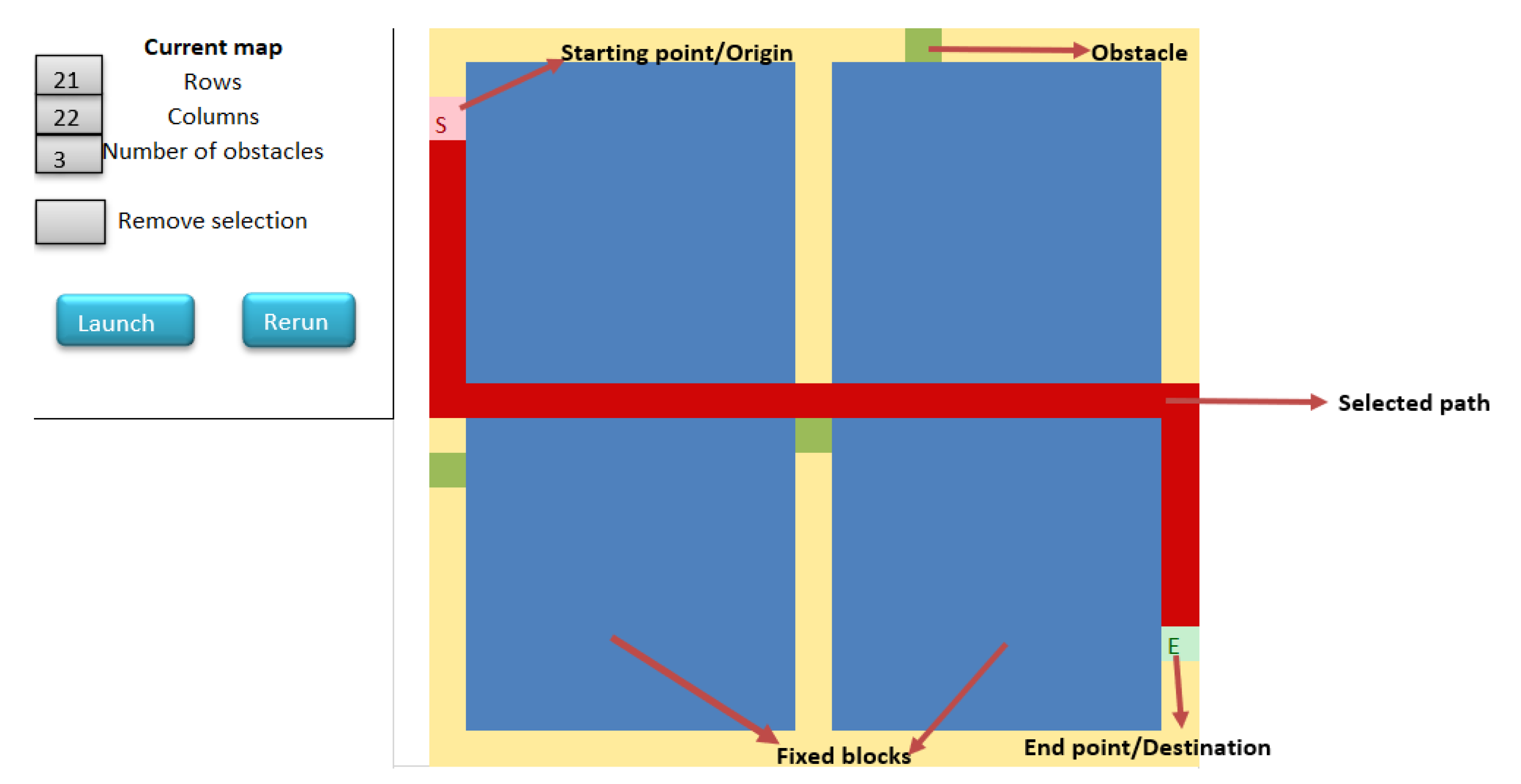
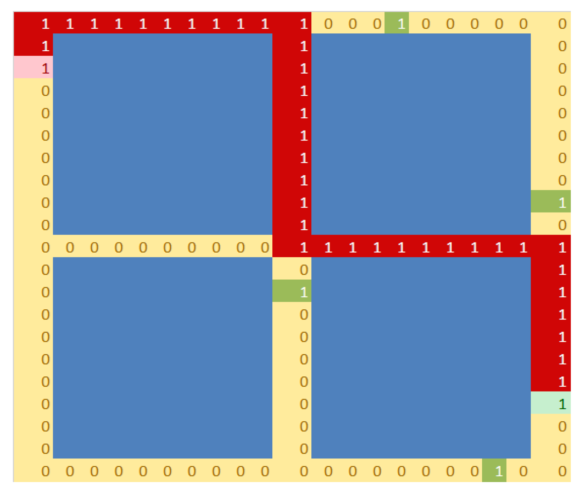
The size of the problem is defined by the number of rows and columns, which are then used to define a transportation area, represented by a rectangle. In Figure 3, an origin is represented by a pink square, and a destination is represented by a light green square. There are two types of obstacles considered in the route-planning problem. Fixed obstacles (or fixed blocks) are represented by blue rectangles, and dynamic obstacles are green squares. The number of dynamic obstacles can be specified, and they are generated at random locations within the transportation area. When the size of the transportation area increases, the complexity of the problem increases significantly, which requires impractical runtimes to determine a solution. For instance, there are three dynamic obstacles in Figure 3. The selected path is represented by a red (thick) line, which connects the starting point and the destination point. The shortest path can be generated on the basis of a shortest-path model or an A-star algorithm to avoid collision with all obstacles (fixed and dynamic) on the grid map. To remove irrelevant data from consideration, a data-encoding process is applied. A transportation area with 21 rows × 21 columns is used in Figure 4 to illustrate the encoding scheme.
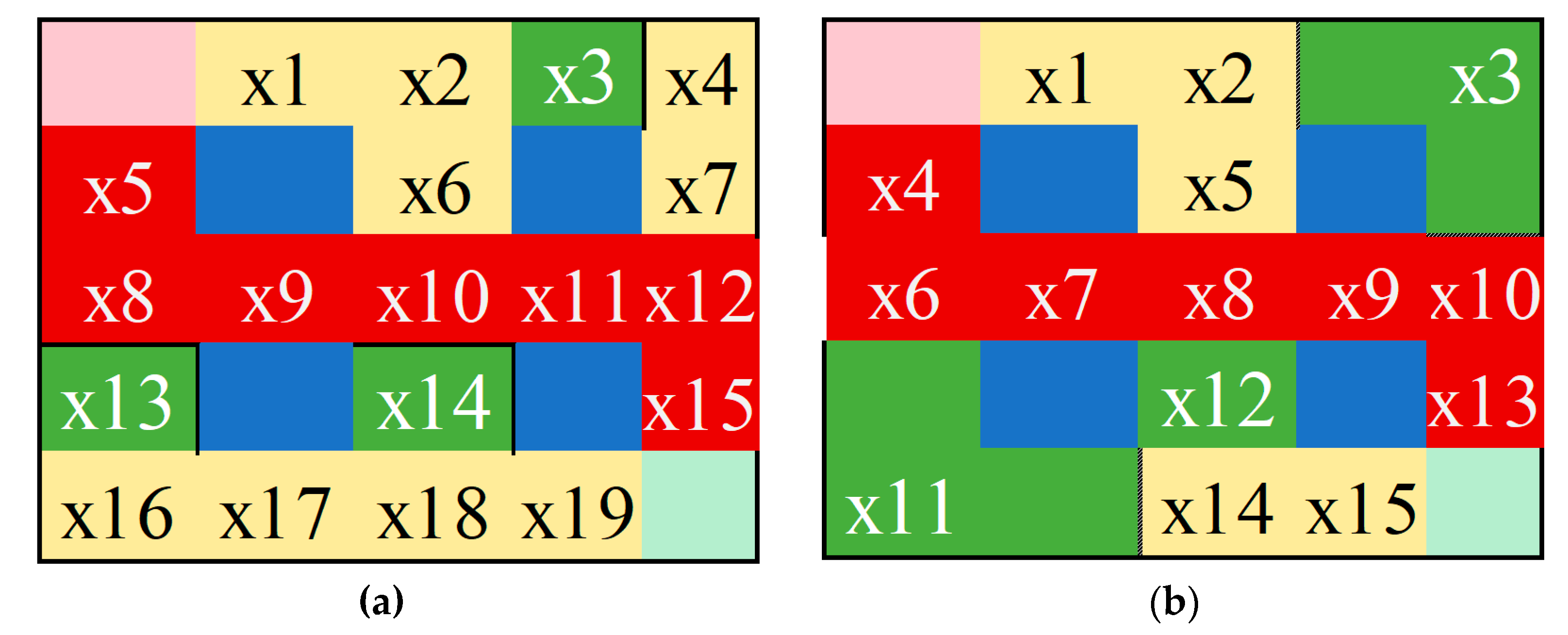
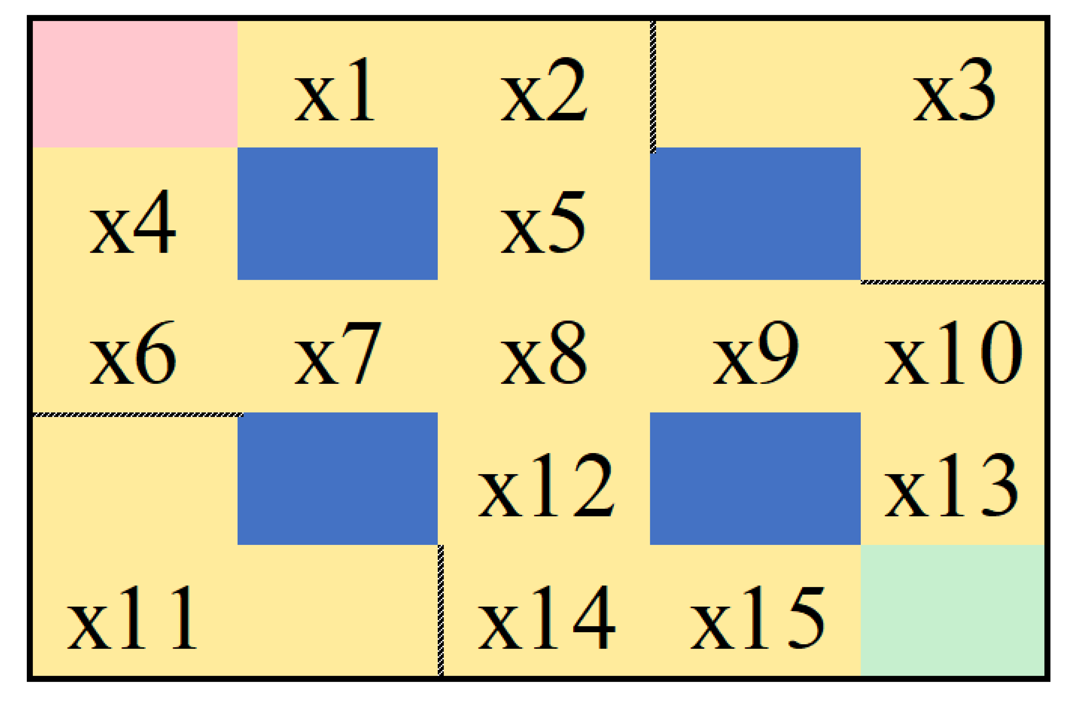
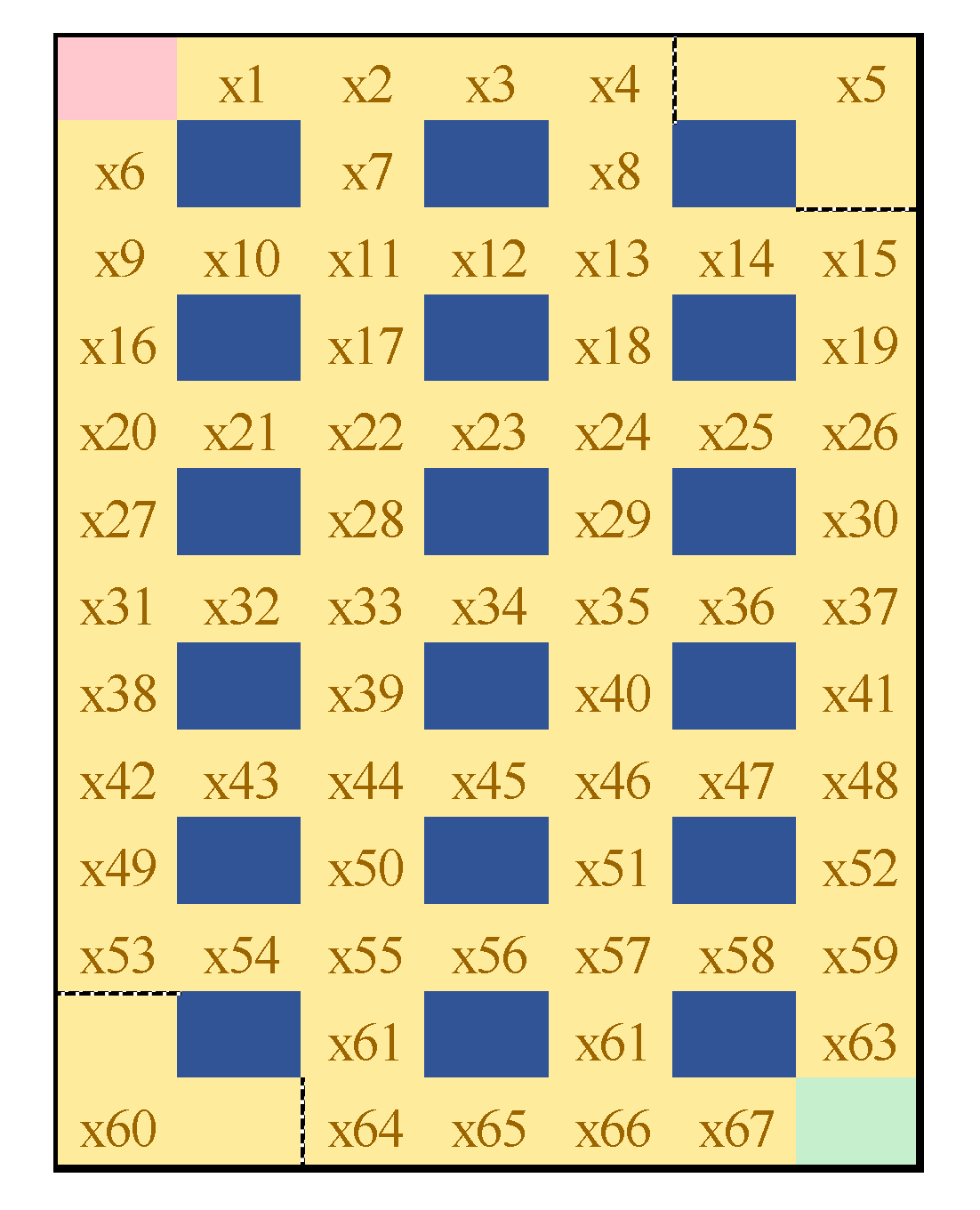
To distinguish between different components within a transportation area, each cell is encoded using the following logic: a cell is encoded with “1” if it represents an origin, a destination, or an obstacle; and encoded with “0” otherwise. Note that fixed obstacles exist permanently and can be omitted from the model. Because a dynamic obstacle located on a line segment blocks the whole segment, an improved encoding scheme is proposed to remove noise from the input data. All cells from a blocked segment are encoded with “1”. Each segment is named as shown in Figure 5. This encoding scheme reduces the combination of input data and greatly reduces the amount of computation required. The output of the ANN is the selected route, which consists of a series of cells from the origin to the destination. The selected route is encoded with a number (e.g., 0, 1, 2) that is used to represent a path identifier (ID). In Figure 4 and Figure 5, the selected path is represented by a red (thick) line that connects the origin to the endpoint. The path is generated using the A-star algorithm to avoid collisions with three obstacles, which exist on segments ×3, ×13, and ×14. However, the obstacles are located in segments at the upper-right corner or lower-left corner. Both entire segments at the corner are blocked the same time, such as ×3, ×4, and ×7 and ×13, ×16, and ×11. Hence, we can group them to become a segment, as shown in Figure 5b. An example of an input dataset is shown as sample 1 in Figure 6, where the selected path was encoded as type 4.
5. Transportation Environment
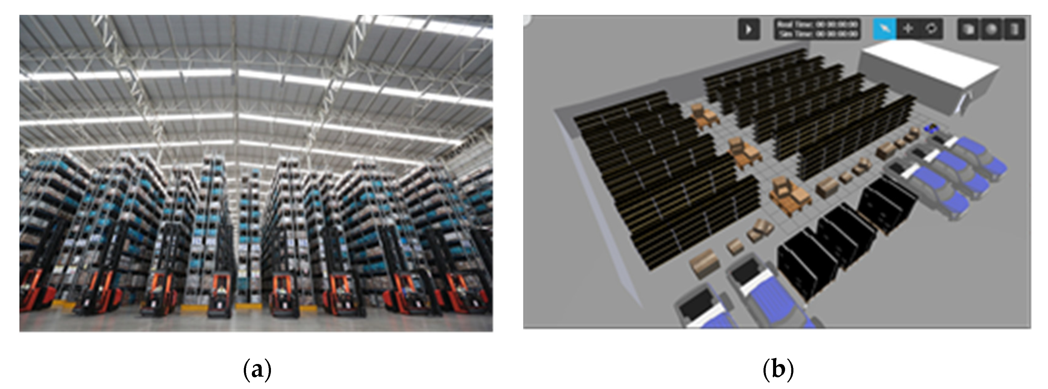
In this project, a distribution center (DC) of one of the top full-cycle construction product suppliers in Thailand was used as a model for creating a transportation area. The DC consists of five sub-DCs that stock different types of products. The overall capacity is more than 100,000 pallets. Because a large volume of product supply needs to be processed, each warehouse has its own operation system that is independent from the others to handle a large volume of product flow daily. The operation flow begins from a planning department that provides tasks to each warehouse. Next, each warehouse prepares its own product delivery plan according to the received orders; then, the products are delivered to a logistic department at DC2 where the consolidation and pickup processes occur. Figure 7a shows a very narrow aisle layout within DC2. To test the movement of an AGV, a simulation environment using an integrated framework between the robot operating system (ROS) and Gazebo was created. Within the framework, the positions of AGVs could be monitored and commands that control the movement of AGVs could be issued through ROS topics. The simulated environment was used to test the movement of an AGV to ensure that it would not collide with other objects within the environment. Figure 7b shows a simulated environment of an internal layout at DC2.
6. Dynamic Route-Planning System and Computational Results with Managerial Insights
In this section, the details of a dynamic routing system and computational results of the proposed methodologies for dynamic route planning are provided.
6.1. Dynamic Route-Planning System
The routes for movement within a DC are initially determined by the shortest-path model and an A-star algorithm. If the solutions from the A-star algorithm have high accuracy when compared with the solutions from the shortest-path model, the A-star algorithm is used due to the shorter runtime and the computing resources required by the automated guided vehicle. Note that an automated guided vehicle is allowed to carry one shipment at a time, due to the standard size of the pallet that can be loaded into a cargo. The input data, which include real-time positions of obstacles, as well as the generated routes, are collected as a training dataset. Once there are sufficient training datasets, an ANN model for a dynamic routing problem is created and used to determine the routing solution. The quality of the solutions from the ANN model needs to be tested with the solutions from the shortest-path model on a regular basis. A requirement is specified according to the accuracy of the ANN model; if the accuracy falls below 95%, the ANN model needs to be updated.
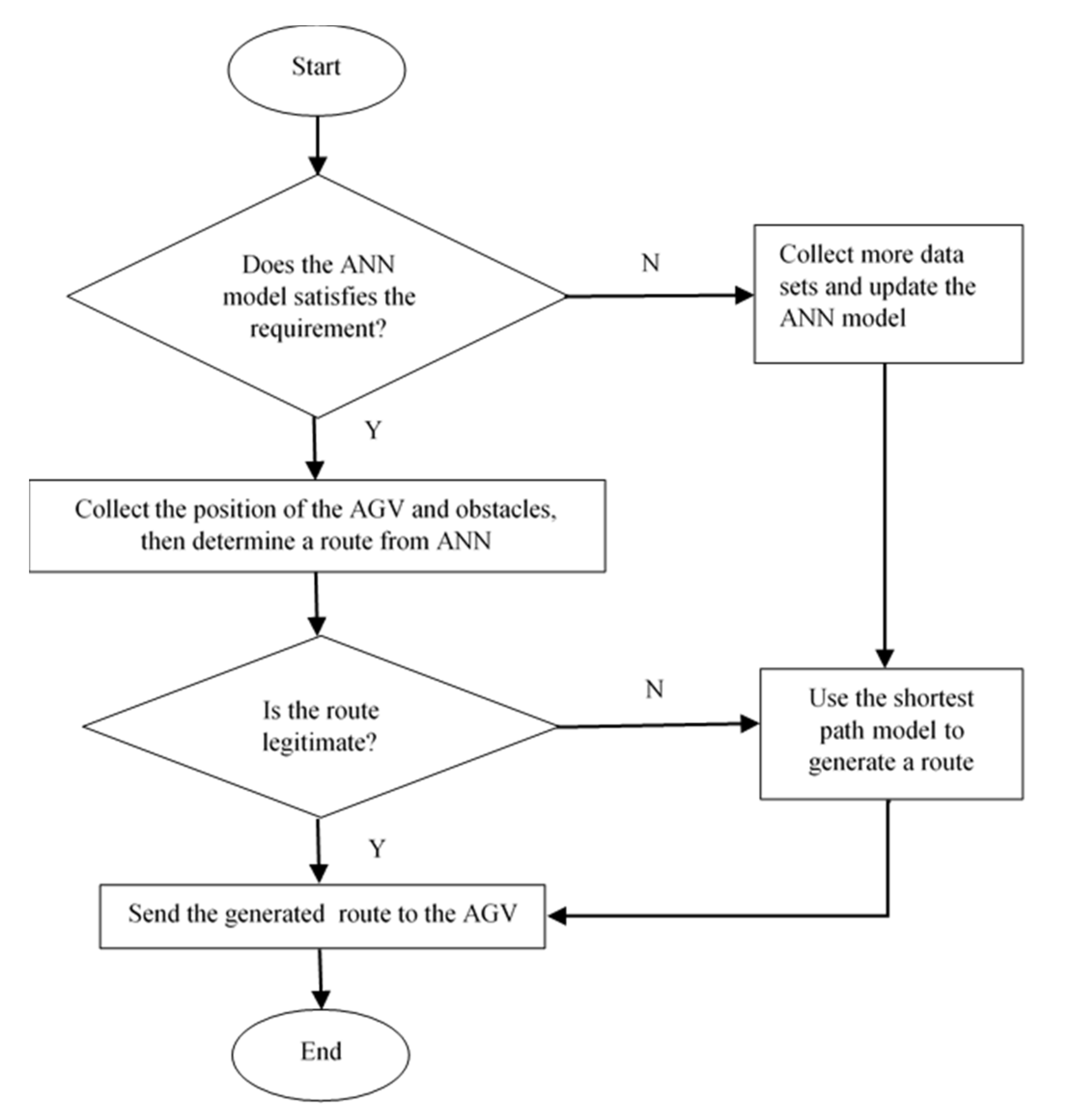
Note that, for any internal movement within a DC, the gap between aisles is narrow; as a result, passing obstacles is not possible. If the path segment contains an obstacle, it is excluded from consideration. Moreover, to consider real-time obstacles in the planning process, the route is generated using the logic provided in Figure 8. At a starting point, a route is generated and used to guide the movement of the vehicle. When an automated guided vehicle reaches an intersection, the positions of obstacles are retrieved. If the positions are unchanged or not on the generated path, the route does not need an update; otherwise, the route needs to be regenerated.
6.2. Computational Results and Managerial Insight
In this section, computational results based on an internal warehouse environment with different sizes are presented.
6.2.1. Computational Results from a Layout with Four Storage Racks and 15 Segments
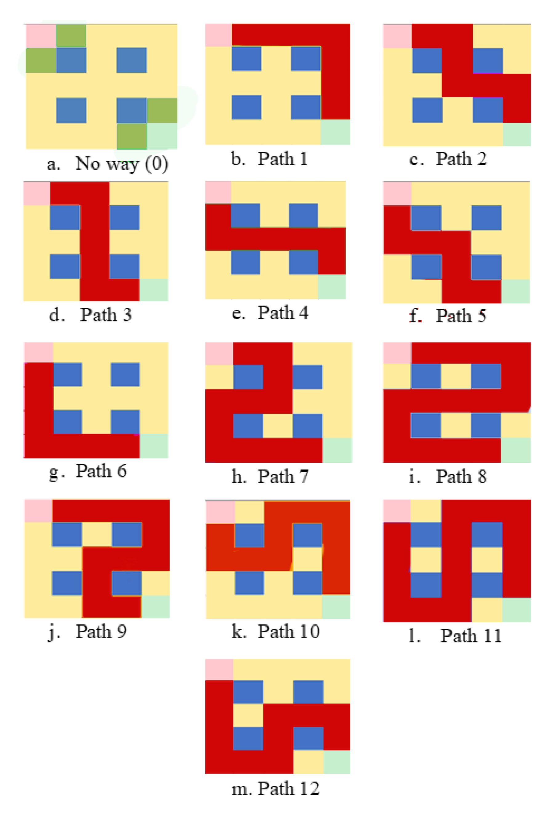
The layout of an internal DC environment described in Section 5 was used as a transportation area for the implementation of the ANN model. Initially, a sample layout consisting of four storage racks with 15 segments was used to test the performance of the proposed approach. The definition of all path segments is shown in Figure 9. Note that the path segments at each corner were combined. The test data were encoded and solved by the A-star algorithm and the shortest-path model. The results from both approaches were the same in all cases, which shows that the performance of the A-star algorithm is acceptable. There were 13 types of paths generated in the solutions, as shown in Figure 10. Each type was assigned an ID; note that “no way” represents a case where a path between the origin and the destination could not be found. Table 2 reports the number of cases for each path type.
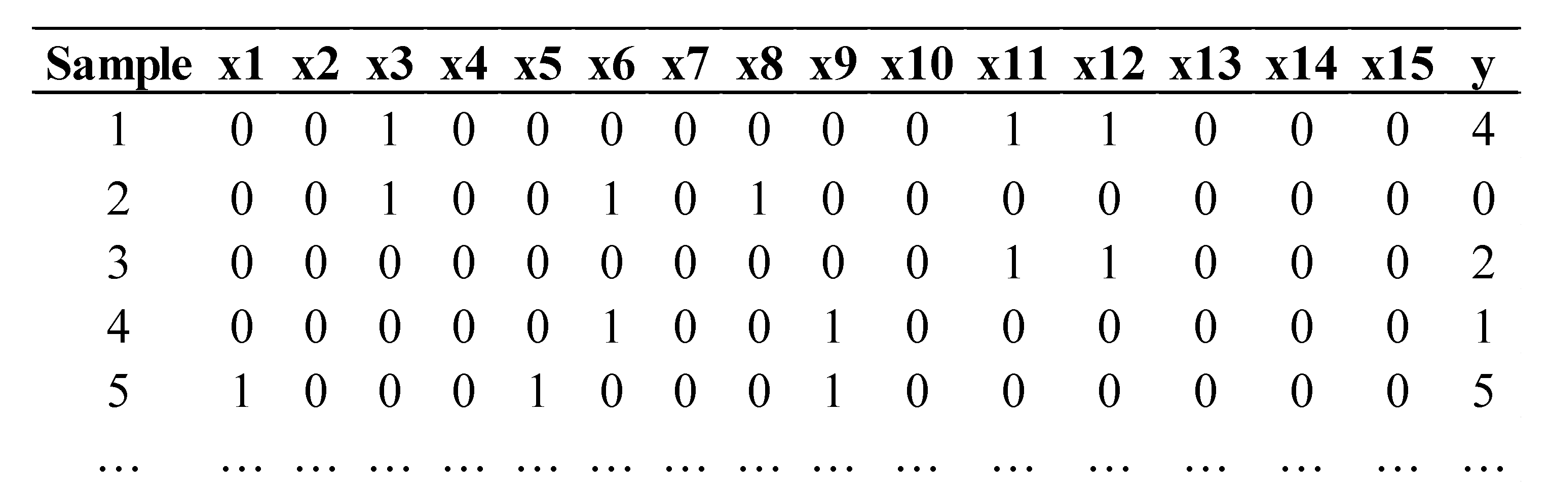
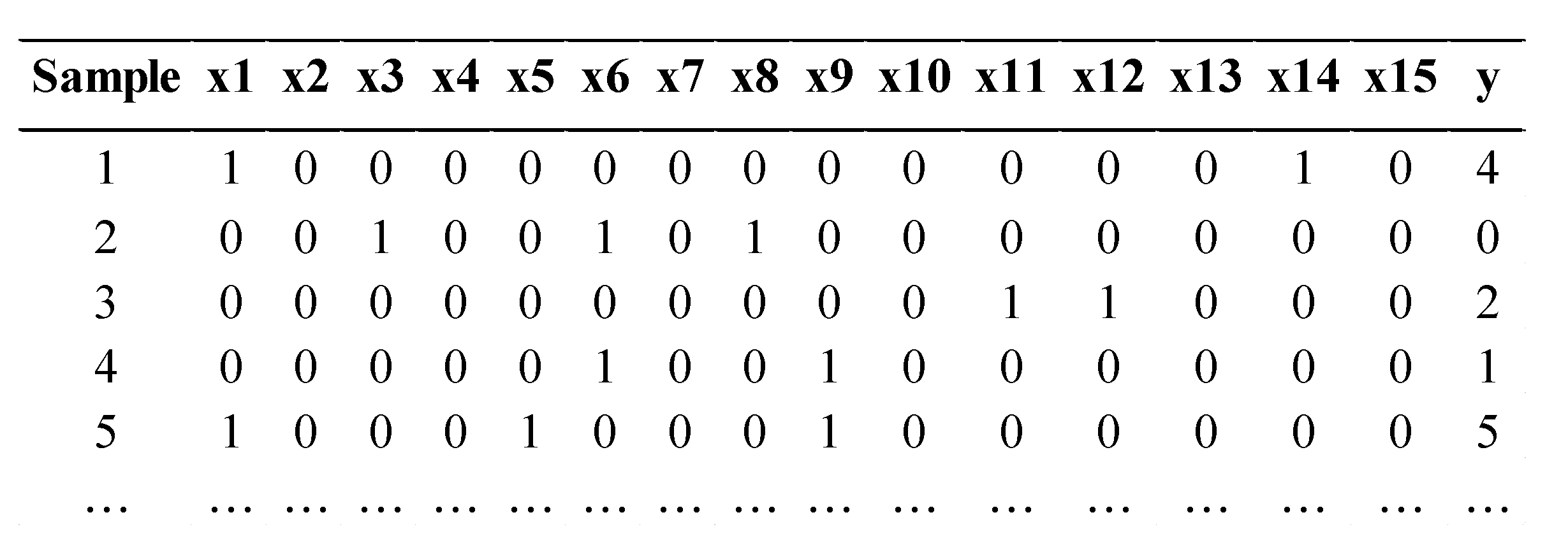
From Table 2, it can be seen that only seven types of paths were significant; the remainder could be considered as outliers and were removed from consideration. The 375 samples were separated into 80% training and 20% testing datasets. An example of encoded input data is shown in Figure 11, where x1 to x15 represent the path segments that have obstacles, and y represents the selected path ID. The structure of the ANN, which is defined by the number of nodes in hidden layers, also affects the accuracy of the ANN model. There are three rules of thumb for determining the number of nodes. The number of hidden nodes should be between the number of input features and the number of target classes, should be equal to the sum of two-thirds of the input features and the size of the output layer, or should be less than double the number of input features. The number of hidden nodes in each experiment should be varied by two or three units. The number of samples for training should be more than 10 times the number of ANN weights [25], which are defined by the equation, numweights = (i +o) × h [26], where i represents the number of input nodes, o is the number of output nodes, and h is the number of nodes in hidden layers.
In this research, the training stage was limited to 1000 iterations. The performance was measured using the mean squared error (MSE), where the target was set to 0. The training function for an ANN’s input layer was based on a “logsig” function, while, for an output layer, it was based on a “purelin” function. A network training function based on a “trainbr” function was used for other layers. The training time was limited to 2 h. The remaining parameters were set on the basis of the “default setting” from the Neural Networks MATLAB toolbox. The accuracy percentages from the training and testing phases, using different datasets (with 200 or 300 samples), are summarized in Table 3. The results were achieved after the training stage reached 1000 epochs. In Table 3, the training accuracy percentage varies with the ANN structural configuration (number of nodes and layers) and the number of training samples. When increasing the number of samples beyond 300 samples, the ANN model required a longer training time; however, the model accuracy was not significantly improved. Hence, 300 samples were used to build the ANN.
Increasing the number of nodes can help improve the accuracy; however, using too many nodes can cause an overfitting issue. This can be seen when comparing configurations (15-8-7) and (15-10-7). Both configurations contained one input layer with 15 nodes, one hidden layer with eight (configuration (15-8-7)) or 10 (configuration (15-10-7)) nodes, and seven nodes in the output layer. Although, configuration (15-10-7) had more nodes, its testing accuracy was 91.7% as opposed to 96.7% (the testing accuracy of configuration (15-8-7)). Moreover, as shown in Table 3, by increasing the number of training data samples from 200 to 300, the accuracy of the configuration (15-8-7) was improved from 85% to 96.7% and that of the configuration (15-10-7) was improved from 75% to 91.7%. Hence, more training samples used resulted in better testing accuracy. The best configuration (15-8-7-7), with a testing accuracy percentage of 98.3%, was used to predict future robot paths for a layout consisting of four storage racks with 15 segments.
6.2.2. Computational Results from a Layout with 18 Storage Racks and 67 Segments
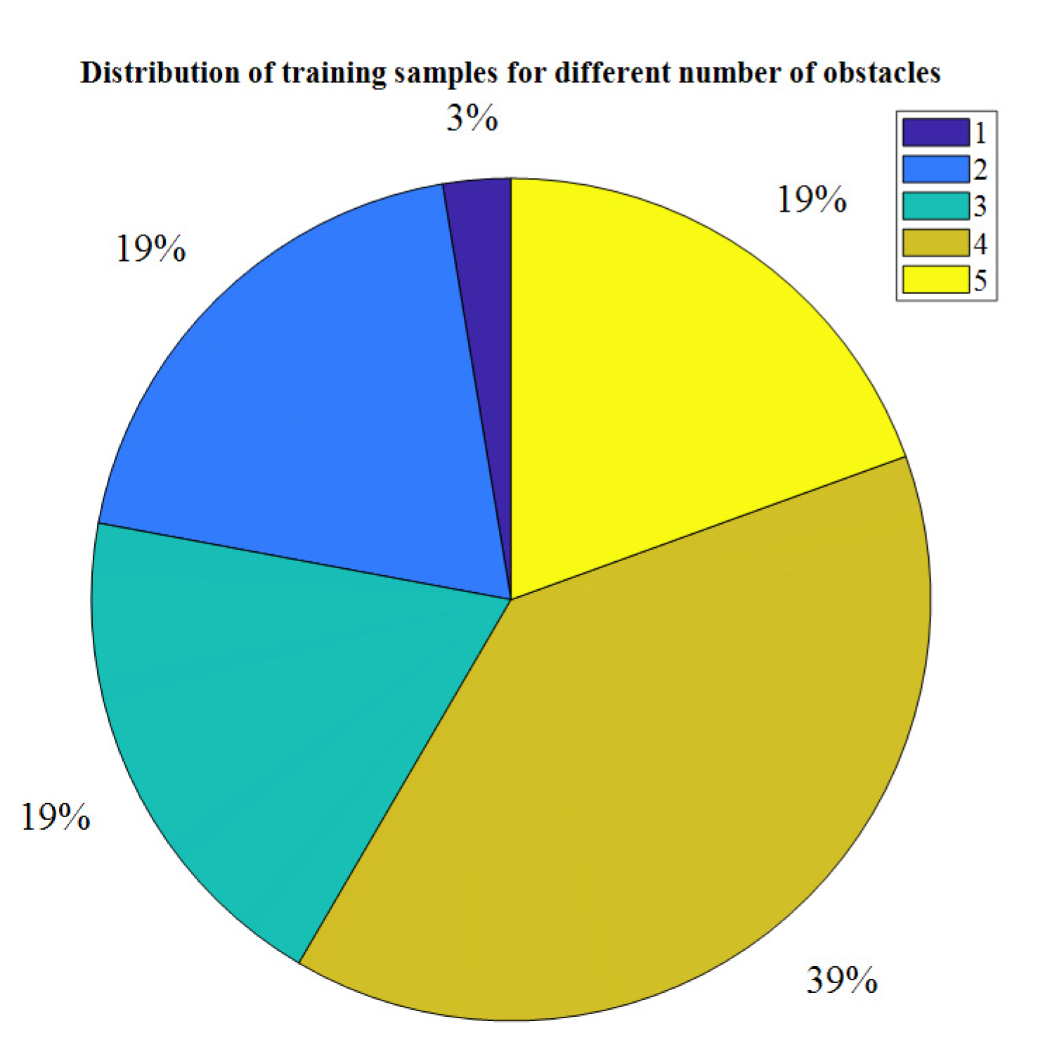
Next, using the data collected from a distribution center (DC), an internal layout with 18 storage racks was created, as shown in Figure 12. There were 67 path segments after combining the segments at the corners. From an observation of an actual operation at the DC, the number of vehicles (folk lifts) working in the DC varies from one to five, with an average of four. Figure 13 shows the distribution of training samples for different numbers of obstacles according to the considered layout. The samples with four obstacles had the highest percentages (39%), while the percentage of samples with two, three, or five obstacles was 19%. The lowest percentage was 3% for samples with one obstacle.
Table 4 summarizes the effect of the number of training samples and ANN configuration on the testing accuracy when a layout from a retail warehouse was used. There were 67 variables in the input layer, corresponding to 67 segments of the layout, and 21 nodes, which represented 21 types of paths generated by the output layer. The number of hidden layers and the number of nodes in each layer were varied to achieve the configuration with the best accuracy. The training accuracy reached more than 90% for all cases, but the testing percentages were different between ANN configurations as a function of the number of samples used for training the ANN. As shown in Table 4, on average, the training accuracy percentages for cases with 1448 and 1000 samples were at the same level for all ANN configurations. However, the average testing accuracy for the case with 1448 samples (95.48%) was higher than that for the 1000-sample case (94.72%).
In addition to the number of samples, the ANN configuration, defined by the number of hidden layers and nodes, also affects the accuracy. Using an inadequate number of nodes in the hidden layers results in an underfitting issue. Underfitting occurs when an ANN is not able to construct an adequate configuration from a dataset. By providing a sufficient number of nodes in each hidden layer, the accuracy percentage can be improved. Hence, as shown in Table 4, the accuracy of an ANN with configuration (67-67-21) was higher than the percentage of an ANN with configuration (67-60-21). Similarly, the accuracy percentage of an ANN with configuration (67-67-21-21), which was the ANN configuration with two hidden layers that had the highest accuracy percentage (97.93%), was higher than the accuracy percentage of an ANN with configuration (67-70-21), which was the best ANN configuration (96.90%) with one hidden layer.
However, having too many nodes in the hidden layers can cause an overfitting issue, where an ANN is not able to generalize the model to identify an output for new input data. Hence, the testing accuracy is deteriorated. For example, when the number of nodes in the hidden layer of an ANN configuration (67-70-21) was increased from 70 to 73 (ANN configuration (67-73-21)), the testing accuracy dropped from 96.79% to 93.79%. Similarly, when considering ANNs with two hidden layers, the testing accuracy of an ANN with configuration (67-67-21-21) (97.93%) was better than the testing accuracy of ANNs with configurations (67-67-30-21) (97.24%) and (67-70-40-21) (96.55%). The highest testing accuracy for cases with 1000 and 1448 samples was 96.5% and 97.93%, respectively, generated by an ANN with configuration (67-70-30-21). Both cases had more than 95% accuracy, which is a criterion for using the ANN model mentioned in Section 6.1. However, the results for the case with 1448 samples were more robust; as a result, the ANN configuration (67-70-30-21) with 1448 training samples was implemented in the dynamic routing system.
7. Conclusions
In this research, the focus was on applying Industry 4.0 technology, related to big data analytics, to a route-planning operation of automated navigation within a warehouse. Route-planning methodologies for a dynamic routing problem with the consideration of real-time obstacles are proposed. An optimization model and a heuristic methodology based on an A-star algorithm were used to generate the routes. Machine learning models using an ANN were developed on the basis of generated datasets using the internal layout of a distribution warehouse. A simulation environment using Gazebo was developed and used for testing the implementation of the route-planning system.
Computational results showed that the proposed machine learning methodologies were able to generate routes with testing accuracy up to 98% for a practical internal layout of a warehouse with 18 storage racks and 67 path segments. Managerial insights into how the machine learning configuration can be selected were also provided. The route-planning system can be used to generate routes for different types of AGVs in real time. This is beneficial to the transportation industry, since there will be a direct reduction in labor cost and an increase in operational efficiency, which is essential to be competitive in today’s business environment. A limitation of our proposed approach is based on the required training datasets for the ANN. If the datasets need to be collected from an actual operation, this might require a long data collection period. However, simulated datasets can also be used, which can help accelerate the ANN training process. A possible future research area includes the consideration of other routing problems such as the vehicle routing problem. In this research, each AGV was assumed to make one stop according to the internal movement within a warehouse. However, in a typical vehicle routing problem, a vehicle has larger capacity and can make multiple stops. This requires the consideration of demands and vehicle capacity in an ANN training process, where suitable data encoding for input and output datasets need to be determined.
Author Contributions
Conceptualization, N.N.; data curation, T.T.H. and D.N.D.; funding acquisition, N.N.; methodology, N.N., T.T.H. and D.N.D.; project administration, D.N.D. and N.N.; software, N.N., T.T.H. and D.N.D.; writing—original draft, T.T.H. and D.N.D.; writing—review and editing, N.N., T.T.H. and D.N.D. All authors have read and agreed to the published version of the manuscript.
Funding
This research was funded by Thammasat University.
Acknowledgments
This study was supported by the Thammasat University Research Fund, Contract No. TUGR 2/33/2562.
Conflicts of Interest
The authors declare no conflict of interest.
References
- Palka, D.; Ciukaj, J. Prospects for development movement in the industry concept 4.0. Multidiscip. Asp. Prod. Eng. 2019, 2, 315–326. [Google Scholar] [CrossRef] [Green Version]
- AI and Robotics Automation in Consumer—Driven Supply Chains: A Rapidly Evolving Source of Competitive Advantage. PA Consulting Group and the Consumer Goods Forum. 2018. Available online: https://www.theconsumergoodsforum.com/wp-content/uploads/2018/04/201805-CGF-AI-Robotics-Report-with-PA-Consulting.pdf (accessed on 1 June 2018).
- D’Andrea, R.; Wurman, P. Future challenges of coordinating hundreds of autonomous vehicles in distribution facilities. In Proceedings of the 2008 IEEE International Conference on Technologies for Practical Robot Applications, Woburn, MA, USA, 10–11 November 2008; pp. 80–83. [Google Scholar]
- Liu, X.; Gong, D. A comparative study of A-star algorithms for search and rescue in perfect maze. In Proceedings of the 2011 International Conference on Electric Information and Control Engineering, Wuhan, China, 25–27 March 2011; pp. 24–27. [Google Scholar]
- ElHalawany, B.M.; Abdel-Kader, H.M.; TagEldeen, A.; Elsayed, A.E.; Nossair, Z.B. Modified a* algorithm for safer mobile robot navigation. In Proceedings of the 2013 5th International Conference on Modelling, Identification and Control (ICMIC), Tianjin, China, 13–15 July 2019; pp. 74–78. [Google Scholar]
- Contreras-González, A.-F.; Hernández-Vega, J.-I.; Hernández-Santos, C.; Palomares-Gorham, D.-G. A method to verify a path planning by a back-propagation articial neural network. In Proceedings of the LANMR, Puebla, Mexico, 15 August 2016; pp. 98–105. [Google Scholar]
- Zhang, Y.; Li, L.-l.; Lin, H.-C.; Ma, Z.; Zhao, J. Development of Path Planning Approach Based on Improved A-star Algorithm in AGV System. In Proceedings of the International Conference on Internet of Things as a Service, Taichung, Taiwan, 20–22 September 2017; pp. 276–279. [Google Scholar]
- Gochev, I.; Nadzinski, G.; Stankovski, M. Path Planning and Collision Avoidance Regime for a Multi-Agent System in Industrial Robotics. Mach. Technol. Mater. 2017, 11, 519–522. [Google Scholar]
- Mohan, L.J.; Ignatious, J. Navigation of Mobile Robot in a Warehouse Environment. In Proceedings of the 2018 International Conference on Emerging Trends and Innovations In Engineering And Technological Research (ICETIETR), Arakkunnam, India, 11–13 July 2018; pp. 1–5. [Google Scholar]
- Kurdi, M.M.; Dadykin, A.K.; Elzein, I.; Ahmad, I.S. Proposed system of artificial Neural Network for positioning and navigation of UAV-UGV. In Proceedings of the 2018 Electric Electronics, Computer Science, Biomedical Engineerings’ Meeting (EBBT), Istanbul, Turkey, 18–19 April 2018; pp. 1–6. [Google Scholar]
- Zhang, Y.; Zhang, Y.; Liu, Z.; Yu, Z.; Qu, Y. Line-of-Sight Path Following Control on UAV with Sideslip Estimation and Compensation. In Proceedings of the 2018 37th Chinese Control Conference (CCC), Wuhan, China, 25–27 July 2018; pp. 4711–4716. [Google Scholar]
- Flórez, C.A.C.; Rosário, J.M.; Amaya, D. Control structure for a car-like robot using artificial neural networks and genetic algorithms. Neural Comput. Appl. 2018, 32, 1–14. [Google Scholar]
- Zhong, X.; Tian, J.; Hu, H.; Peng, X. Hybrid Path Planning Based on Safe A* Algorithm and Adaptive Window Approach for Mobile Robot in Large-Scale Dynamic Environment. J. Intell. Robot. Syst. 2020, 99, 1–13. [Google Scholar] [CrossRef]
- Bhadoria, A.; Singh, R.K. Optimized angular a star algorithm for global path search based on neighbor node evaluation. Int. J. Intell. Syst. Appl. 2014, 6, 46. [Google Scholar] [CrossRef] [Green Version]
- Zhang, Z.; Zhao, Z. A multiple mobile robots path planning algorithm based on A-star and Dijkstra algorithm. Int. J. Smart Home 2014, 8, 75–86. [Google Scholar] [CrossRef] [Green Version]
- Kusuma, M.; Machbub, C. Humanoid robot path planning and rerouting using A-Star search algorithm. In Proceedings of the 2019 IEEE International Conference on Signals and Systems (ICSigSys), Bandung, Indonesia, 16–18 July 2019; pp. 110–115. [Google Scholar]
- Ruiz, E.; Soto-Mendoza, V.; Barbosa, A.E.R.; Reyes, R. Solving the open vehicle routing problem with capacity and distance constraints with a biased random key genetic algorithm. Comput. Ind. Eng. 2019, 133, 207–219. [Google Scholar] [CrossRef]
- Salavati-Khoshghalb, M.; Gendreau, M.; Jabali, O.; Rei, W. An exact algorithm to solve the vehicle routing problem with stochastic demands under an optimal restocking policy. Eur. J. Oper. Res. 2019, 273, 175–189. [Google Scholar] [CrossRef]
- Zhang, H.; Zhang, Q.; Ma, L.; Zhang, Z.; Liu, Y. A hybrid ant colony optimization algorithm for a multi-objective vehicle routing problem with flexible time windows. Inf. Sci. 2019, 490, 166–190. [Google Scholar] [CrossRef]
- Sung, I.; Choi, B.; Nielsen, P. On the training of a neural network for online path planning with offline path planning algorithms. Int. J. Inf. Manag. 2020. [Google Scholar] [CrossRef]
- Pasha, J.; Dulebenets, M.A.; Kavoosi, M.; Abioye, O.F.; Wang, H.; Guo, W. An Optimization Model and Solution Algorithms for the Vehicle Routing Problem With a “Factory-in-a-Box”. IEEE Access 2020, 8, 134743–134763. [Google Scholar] [CrossRef]
- Trachanatzi, D.; Rigakis, M.; Marinaki, M.; Marinakis, Y. A Firefly Algorithm for the Environmental Prize-Collecting Vehicle Routing Problem. Swarm Evol. Comput. 2020, 57, 100712. [Google Scholar] [CrossRef]
- Taccari, L. Integer programming formulations for the elementary shortest path problem. Eur. J. Oper. Res. 2016, 252, 122–130. [Google Scholar] [CrossRef]
- Klancar, G.; Zdesar, A.; Blazic, S.; Skrjanc, I. Wheeled Mobile Robotics: From Fundamentals towards Autonomous Systems; Butterworth-Heinemann: Oxford, UK, 2017. [Google Scholar]
- Baptista, F.D.; Rodrigues, S.; Morgado-Dias, F. Performance comparison of ANN training algorithms for classification. In Proceedings of the 2013 IEEE 8th International Symposium on Intelligent Signal Processing, Funchal, Portugal, 16–18 September 2013; pp. 115–120. [Google Scholar]
- Panchal, G.; Ganatra, A.; Kosta, Y.; Panchal, D. Behaviour analysis of multilayer perceptrons with multiple hidden neurons and hidden layers. Int. J. Comput. Theory Eng. 2011, 3, 332–337. [Google Scholar] [CrossRef] [Green Version]
Figure 1.
Industry 4.0 technology [1].
Figure 1.
Industry 4.0 technology [1].

Figure 2.
A feed-forward ANN with a hidden layer.

Figure 3.
A grid map used for route planning.

Figure 4.
A grid map with encoded data.

Figure 5.
A grid map with an improved encoding scheme: (a) the original encoded map; (b) the map after combining corner segments.
Figure 5.
A grid map with an improved encoding scheme: (a) the original encoded map; (b) the map after combining corner segments.

Figure 6.
An example of encoded input and output data for a dynamic route-planning problem.

Figure 7.
Distribution center 2 (DC2): (a) a very narrow aisle layout at DC2; (b) a simulated environment of an internal layout at DC2.
Figure 7.
Distribution center 2 (DC2): (a) a very narrow aisle layout at DC2; (b) a simulated environment of an internal layout at DC2.

Figure 8.
The logic for generating a dynamic route.

Figure 9.
Layout of an internal distribution center (DC) with 15 path segments.

Figure 10.
Types of generated paths.

Figure 11.
An example of encoded input and output data for an ANN model.

Figure 12.
Internal layout of a DC with 18 storage racks.

Figure 13.
Distribution of training samples for different numbers of obstacles.


Table 1.
A summary of the methods used in key related articles. ANN, artificial neural network.
| No. | Authors | Year | Route Planning | Motion Planning | Automated Robot | Warehouse Application | Use of ANN | Realtime Obstacle |
|---|---|---|---|---|---|---|---|---|
| 1 | Liu and Gong [4] | 2011 | x | x | x | |||
| 2 | ElHalawany et al. [5] | 2013 | x | x | ||||
| 3 | Bhadoria and Singh [14] | 2014 | x | x | x | |||
| 4 | Zhang and Zhao [15] | 2014 | x | x | x | |||
| 5 | Contreras-González et al. [6] | 2016 | x | x | x | |||
| 6 | Zhang et al. [7] | 2017 | x | x | ||||
| 7 | Gochev et al. [8] | 2017 | x | x | x | |||
| 8 | Mohan and Ignatious [9] | 2018 | x | x | x | |||
| 9 | Kurdi et al. [10] | 2018 | x | x | x | x | ||
| 10 | Zhang et al. [11] | 2018 | x | x | x | |||
| 11 | Flórez et al. [12] | 2018 | x | x | x | x | ||
| 12 | Kusuma and Machbub [16] | 2019 | x | x | x | |||
| 13 | Ruiz et al. [17] | 2019 | x | x | ||||
| 14 | Salavati-Khoshghalb et al. [18] | 2019 | x | x | ||||
| 15 | Zhang et al. [19] | 2019 | x | x | ||||
| 16 | Zhong et al. [13] | 2020 | x | x | x | |||
| 17 | Sung et al. [20] | 2020 | x | x | x | |||
| 18 | Pasha et al. [21] | 2020 | x | x | ||||
| 19 | Trachanatzi et al. [22] | 2020 | x | x | ||||
| 20 | This research | 2020 | x | x | x | x | x |
Table 2.
Number of cases for each path type. ID, identifier.
| ID | 0 | 1 | 2 | 3 | 4 | 5 | 6 | Others |
|---|---|---|---|---|---|---|---|---|
| Count | 91 | 32 | 61 | 28 | 67 | 40 | 49 | 7 |
Table 3.
The effect of the number of training sample and ANN configuration on the testing accuracy for a sample layout with 15 segments.
Table 3.
The effect of the number of training sample and ANN configuration on the testing accuracy for a sample layout with 15 segments.
| 200 Samples | 300 Samples | |||
|---|---|---|---|---|
| ANN’s Hidden Layer Topology | Training Accuracy (%) | Testing Accuracy (%) | Training Accuracy (%) | Testing Accuracy (%) |
| 15-5-7 | 93.3 | 70 | 92.5 | 85 |
| 15-8-7 | 100 | 85 | 100 | 96.7 |
| 15-10-7 | 100 | 75 | 100 | 91.7 |
| 15-8-7-7 | 100 | 95 | 100 | 98.3 |
| 15-8-10-7 | 100 | 90 | 100 | 93.3 |
Table 4.
The effect of the number of training samples and ANN configuration on the testing accuracy for an actual layout.
Table 4.
The effect of the number of training samples and ANN configuration on the testing accuracy for an actual layout.
| ANNs | 1000 | 1448 | ||
|---|---|---|---|---|
| Training | Testing | Training | Testing | |
| 67-60-21 | 99.7 | 94.00 | 99.7 | 94.83 |
| 67-67-21 | 99.7 | 93.50 | 99.7 | 95.52 |
| 67-70-21 | 99.7 | 96.00 | 99.7 | 96.90 |
| 67-73-21 | 99.7 | 93.50 | 99.7 | 93.79 |
| 67-67-21-21 | 99.7 | 95.50 | 99.7 | 97.93 |
| 67-67-30-21 | 99.7 | 96.00 | 99.7 | 97.24 |
| 67-70-30-21 | 99.7 | 96.50 | 99.7 | 97.93 |
| 67-70-40-21 | 99.25 | 96.00 | 99.65 | 96.55 |
| 67-67-21-10-21 | 90.00 | 91.50 | 91.19 | 88.62 |
Publisher’s Note: MDPI stays neutral with regard to jurisdictional claims in published maps and institutional affiliations. |
© 2020 by the authors. Licensee MDPI, Basel, Switzerland. This article is an open access article distributed under the terms and conditions of the Creative Commons Attribution (CC BY) license (http://creativecommons.org/licenses/by/4.0/).
Share and Cite
MDPI and ACS Style
Nguyen Duc, D.; Tran Huu, T.; Nananukul, N. A Dynamic Route-Planning System Based on Industry 4.0 Technology. Algorithms 2020, 13, 308. https://0-doi-org.brum.beds.ac.uk/10.3390/a13120308
AMA Style
Nguyen Duc D, Tran Huu T, Nananukul N. A Dynamic Route-Planning System Based on Industry 4.0 Technology. Algorithms. 2020; 13(12):308. https://0-doi-org.brum.beds.ac.uk/10.3390/a13120308
Chicago/Turabian StyleNguyen Duc, Duy, Thong Tran Huu, and Narameth Nananukul. 2020. "A Dynamic Route-Planning System Based on Industry 4.0 Technology" Algorithms 13, no. 12: 308. https://0-doi-org.brum.beds.ac.uk/10.3390/a13120308
Note that from the first issue of 2016, this journal uses article numbers instead of page numbers. See further details here.