Article

Swarm-Based Design of Proportional Integral and Derivative Controllers Using a Compromise Cost Function: An Arduino Temperature Laboratory Case Study

by
P. B. de Moura Oliveira
1,2,*,
John D. Hedengren
3 and
E. J. Solteiro Pires
1
1
Department of Engineering, University of Trás-os-Montes and Alto Douro (UTAD), 5000-801 Vila Real, Portugal
2
Institute for Systems and Computer Engineering, Technology and Science (INESC-TEC), Campus da Faculdade de Engenharia da Universidade do Porto (FEUP), 4200-465 Porto, Portugal
3
Department of Chemical Engineering, Brigham Young University, Provo, UT 84602, USA
*
Author to whom correspondence should be addressed.
Submission received: 25 October 2020 / Revised: 22 November 2020 / Accepted: 27 November 2020 / Published: 30 November 2020
(This article belongs to the Special Issue Algorithms for PID Controller 2019)

Abstract

:
Simple and easy to use methods are of great practical demand in the design of Proportional, Integral, and Derivative (PID) controllers. Controller design criteria are to achieve a good set-point tracking and disturbance rejection with minimal actuator variation. Achieving satisfactory trade-offs between these performance criteria is not easily accomplished with classical tuning methods. A particle swarm optimization technique is proposed to design PID controllers. The design method minimizes a compromise cost function based on both the integral absolute error and control signal total variation criteria. The proposed technique is tested on an Arduino-based Temperature Control Laboratory (TCLab) and compared with the Grey Wolf Optimization algorithm. Both TCLab simulation and physical data show that satisfactory trade-offs between the performance and control effort are enabled with the proposed technique.

1. Introduction

Despite the development of more refined control techniques, the Proportional, Integral, and Derivative (PID) control continues to be ubiquitous for industrial control [1,2]. Given the practical relevance of this type of control, many design methods have been proposed since the pioneering work developed by Ziegler and Nichols [3]. PID tuning rules were developed for specific aspects, such as: Control modes (P, PI, PD, or PID); types of system model characteristics or forms (first order plus time delay, second order plus time delay, non-minimum phase, oscillatory, etc.); PID controller structure (parallel, series, with filters, with two-degrees of freedom, etc.); and anti-windup schemes [4,5,6,7]. The PID control practical relevance also motivates inclusion in most introductory feedback control courses, for example [8].
Artificial neural networks, fuzzy logic, and evolutionary computation have been successfully applied for the PID controller design. The ever-increasing computational power enables a fast practical implementation of computer-based PID controller design methodologies. Optimization-based techniques have advantages over classical tuning methodologies, as the former can be used independently of both system dynamics and PID control structure. Examples of the most well-established population-based algorithms which seek inspiration from natural phenomena are: Genetic Algorithm (GA) [9], Ant-Colony Optimization, (ACO) [10], Genetic Programming (GP) [11], Differential Evolution (DE) [12], Particle Swarm Optimization (PSO) [13], Cuckoo Search Algorithm (CS) [14], Firefly Algorithm (FA) [15], Glowworm Swarm Optimization (GSO) [16], Gravitational Search Algorithm (GSA) [17], Grey Wolf Optimization (GWO) [18,19,20,21], and Elephant Herding Optimization (EHO) [22]. From this set, the ones most used within control design applications are GA [23,24] and more recently the PSO [25,26]. PSO has been improved as a result of significant research effort [27,28].
A commonly used argument against using bio-inspired and nature inspired metaheuristics over classical PID design methods is that these also require the adjustment of parameters prior to the optimization procedure. An advantage of the classical PSO algorithm is fewer adjustable heuristic settings compared with the basic GA. Moreover, PSO is more straightforward to implement than a GA. As the proposed technique aims to be simple to configure, the PSO algorithm is the selected optimization tool used in this study. Moreover, the proposed technique control performance is compared with a more recently introduced metaheuristic: The Grey Wolf Optimization proposed by [18].
There is an increasing pedagogical and research benchmark interest in pocket-sized and portable-based control experiments, as revealed by the following examples in [29,30,31,32,33,34]. Microcontrollers enable a wide range of pocket-size laboratories as common tools both for teaching/learning purposes, as well as for control engineering practitioners testing controller designs. The paradigm is shifting from monolithic laboratory experiments that require significant resources to take-home and modular experiments. The Temperature Control Laboratory (TCLab) proposed by [35,36,37,38] is used to teach PID control to undergraduate engineering students [39,40]. The TCLab is a low-cost Arduino-based lab which is a pocket-sized, plug-and-play kit, meaning that it does not require the user to perform the assembly. This is quite advantageous for computer-based control courses in which the primary goal is to test the identification and control techniques rather than hardware assembly. The TCLab is programmed using different environments, such as: Python, MATLAB®/SIMULINK®, and GNU Octave. Moreover, a wide range of open-source supporting materials, including programs, videos, and tutorials are freely available in [24].
The PSO was applied to identify a first order plus time delay model for the TCLab kit in [39,40]. In this paper, the PSO design of PID controllers based on an additive compromise cost function involving the Integral Absolute Error (IAE) and Total Variation (TV) is proposed. This technique is validated both with simulation and practical results obtained with the TCLab. The results obtained with the proposed technique are compared with the ones obtained with the GWO algorithm and classical tuning techniques. The novel contributions of this paper are highlighted in the following points:
  • New formulation for an additive compromise (or aggregated) cost function involving the Integral Absolute Error (IAE) and Total Variation (TV). Major control design criteria concern optimizing set-point tracking and disturbance rejection, while minimizing the control signal variation. This proposed technique significantly simplifies the PID controller design procedure combining these criteria into a single-objective optimization formulation.
  • PSO algorithm to design PID controllers that minimize a cost function weighting IAE and TV. A simple PSO algorithm constitutes an excellent design tool for the PID controller, with practical interest for control engineers. The proposed technique is compared with the original GWO algorithm, in a TCLab temperature control case study, providing a similar control performance.
  • Both the simulation and practical validation with TCLab tests, show an effectiveness to design PID controllers by softening the control signal.
The paper remainder is organized as follows: Section 2 introduces the problem statement. In Section 3, the classical particle swarm optimization algorithm is presented. Section 4 and Section 5 discuss the TCLab main features and results. Finally, Section 6 provides the conclusions and recommendations for future work.

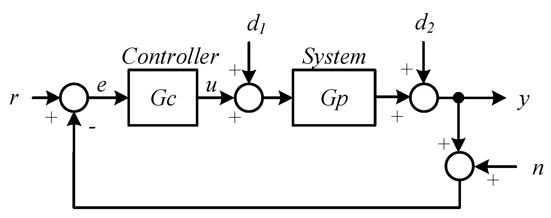
2. PID Control Design: Problem Statement

Consider a general block diagram representation of a closed-loop system in Figure 1, assuming the following representation where r is the reference input (set-point), y is the controlled output, e is the error signal, u is the control output, d1 is a load disturbance, d2 is an output disturbance, n is a noise signal, and Gc and Gp are the controller and process transfer functions.
The ideal feedback control corresponds to obtaining the controlled output equal to the reference input independent of system disturbances. This ideal control is not possible in practice due to disturbances, measurement noise, actuator saturation, and a wide range of other physical limitations. With these limitations, the controlled output should attempt to follow the reference input (Set-Point Tracking, SPT), while rejecting the system disturbances (Disturbance Rejection, DR). In this work, it is assumed that a dynamic model of the system can be identified. In addition to the SPT and DR criteria, it is also important to consider the control effort in the controller design. A relevant research question is: How can a PID controller be designed to achieve the best possible set-point performance while minimizing the control effort?
There are many time-domain criteria to evaluate a controller performance. These criteria frequently involve set-point step responses with the smallest possible values for first overshoot and rise time. An indirect approach to simultaneously minimize several step response indices is using error-based criteria. The most common are the following: Integral of Square Error (ISE), Integral of Absolute Error (IAE), Integral of Time Weighted Absolute Error (ITAE), and Integral Weighted Square Error (ITSE), represented respectively by the following expressions:
ISE = 0 t sim e 2 ( t )   dt
IAE = 0 t sim | e ( t ) | dt
ITAE = 0 t sim t | e ( t ) | dt
ITSE = 0 t sim te 2 ( t ) dt
with tsim representing the simulation time, which should be large enough so that the system-controlled output reaches the steady-state value. Depending on which of these criteria is adopted in the optimization cost function, different PID controller settings are obtained. Among these criteria the most widely used are the ISE, IAE, and ITAE. Time weighting the absolute error penalizes the error as time increases for ITAE, promoting the elimination of small steady-state errors. IAE independently gives the same relevance to errors over time. For this reason, IAE is adopted in this study. A common criterion to measure the control effort is:
E u = 0 t sim | u ( t ) | dt
with u representing the control signal. The control signal smoothness can be evaluated using a Total Variation (TV) index (6), approximated by (7):
TV u = 0 t sim   | du dt | dt
TV u = k = 0 t sim h | u ( k   +   1 )     u ( k ) |
with h representing the measurement sampling interval. The TV criterion is adopted in this study to minimize the control signal variation. It is worthwhile to mention at this point, that all actuators have physical limitations, and it is common that the control signal can vary linearly in the interval [umin,umax], with umin and umax representing the minimum and maximum control signal values, respectively. A realistic controller design for practical implementation should consider specific actuator saturation limits. Measurement noise issues are not addressed in this study.
With two performance criteria selected (IAE and TV), a decision regarding how to use these in the optimization algorithm must be made. The two criteria can be considered as two separate functions within a multi-objective (or many-objective) optimization problem and solved using a PSO Pareto-based approach [41]. However, depending on the number of objectives, the computational burden associated with multicriteria optimization can be significant. After a non-dominated Pareto front is achieved, a decision support system should be used to help the operator decide the appropriate trade-offs from the Pareto front. Considering that just two criteria are used (IAE and TV), a simpler approach uses an additive compromise cost function. This cost function is represented by:
J = α IAE + β   TV
with α and β representing weighting factors determining the relative importance of each criterion. An equivalent single parameter β could also be used if the α value is always fixed to a value of one as done in this paper.

3. Classical Particle Swarm Optimization

The particle swarm optimization algorithm proposed by Kennedy and Eberhart [13] is inspired by the animal swarms social behavior, such as bird flocks and fish schools. The basic notion of the algorithm can be explained using the illustrative example presented in Figure 2.
A swarm is represented with m particles. Each generic particle, i, has dynamics which are characterized by two d-dimension variables x and v, representing respectively, the particle position in space and the corresponding velocity. The swarm is randomly initialized in the search space unless there is specific information regarding the problem. The specific information can be incorporated in the initialization procedure to improve the convergence rate to an optimal solution. Each PSO iteration, t, updates every particle position to a new position. The update is from the sum of a velocity term according to (8) with the velocity evaluated using (9):
x i ( t + 1 ) = x i ( t ) + v i ( t + 1 )
v i ( t + 1 ) = ω   v i ( t ) + c 1 ϕ 1 [ b i ( t )     x i ( t ) ] + c 2 ϕ 2 [ g ( t ) x i ( t ) ]
where bi represents the best position obtained by particle i until the current iteration, t; g represents the best position from the full swarm (global best) or a specific neighborhood (local best). In this study, information is shared among the entire swarm (fully-connected model). As it can be observed from (9), the new velocity value is evaluated by a sum of three parts. The first part ( ω   v i ( t ) ) is the inertia and considers the previous velocity value with a factor, ω, called inertia weight. The second part ( c 1 ϕ 1 [ b i ( t ) x i ( t ) ] ) represents the particle cognitive knowledge update. It is the difference between the particle i individual best position, bi, and the particle current position, xi, multiplied by a cognitive constant c1 and a disturbing random value, ϕ1. The third part ( c 2 ϕ 2 [ g ( t ) x i ( t ) ] ) represents the particle social knowledge update: The difference between the swarm global best position, g, and the particle current position, xi, multiplied by a social constant c2 and a disturbing random value, ϕ2. The same relevance is usually given to the cognitive and social knowledge, and thus, c1 and c2 take the same value (e.g., 2 or 1.49445). The two random numbers, ϕ1 and ϕ2, are uniformly generated in the interval [0, 1]. Algorithm 1 is represented by the following pseudo-code:
Algorithm 1 PSO algorithm
1. t = 0
2. Initiate m,ω
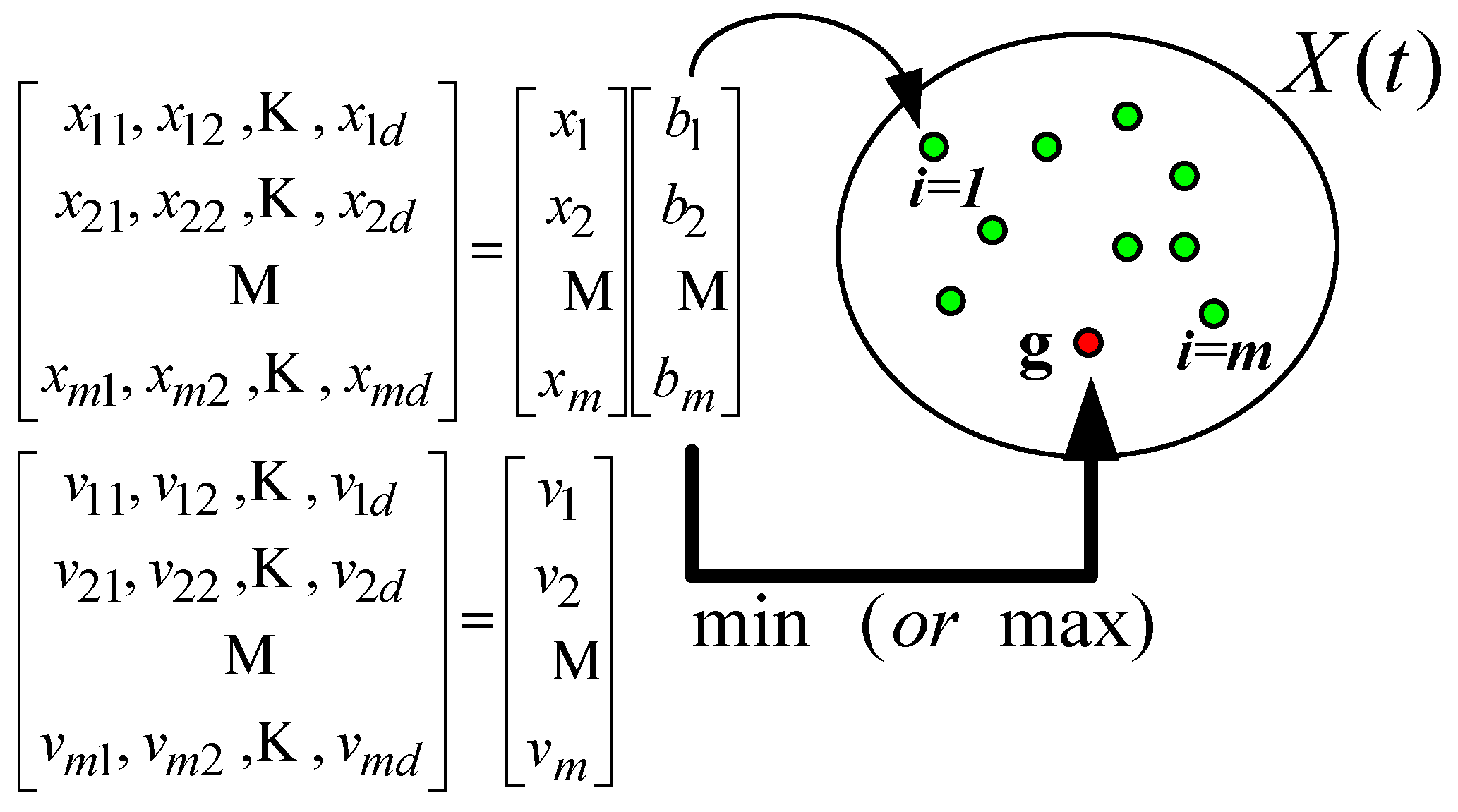
3. Initialize swarm X(t)
4. Evaluate X(t)
while(not (termination criterion))
5. determine personal and global bests
for i = 1 to m
   6. Update vi(t + 1)
   7. Update xi(t + 1)
endfor
8. Update ω
9. t = t + 1
endwhile
As it can be observed from the PSO pseudo-code, this algorithm is conceptually quite simple. Regarding the PSO algorithm parametrization, there are three adjustable parameters: The swarm size, m, the termination criterion and the inertia weight limits. While these parameters are problem dependent, they can easily be selected for most PID control design cases. The swarm size should be large enough to guarantee a diverse solution representation across the search space. The termination criterion is often a pre-defined number of iterations and is adopted in this study. Regarding the inertia weight, it is commonly accepted that it should assume a higher value at the beginning of the search (e.g., ωi = 0.7) and then gradually decreased over the search evolution until it reaches a minimum value (e.g., ωf = 0.4). This inertia weight variation is to establish an important trade-off between space exploration in an early search stage and gradually transition to a global minimum consensus in a final search stage. The inertia weight is linearly decayed between the maximum and minimum values over the search iterations. However, other approaches can also be used (e.g., see [42]).

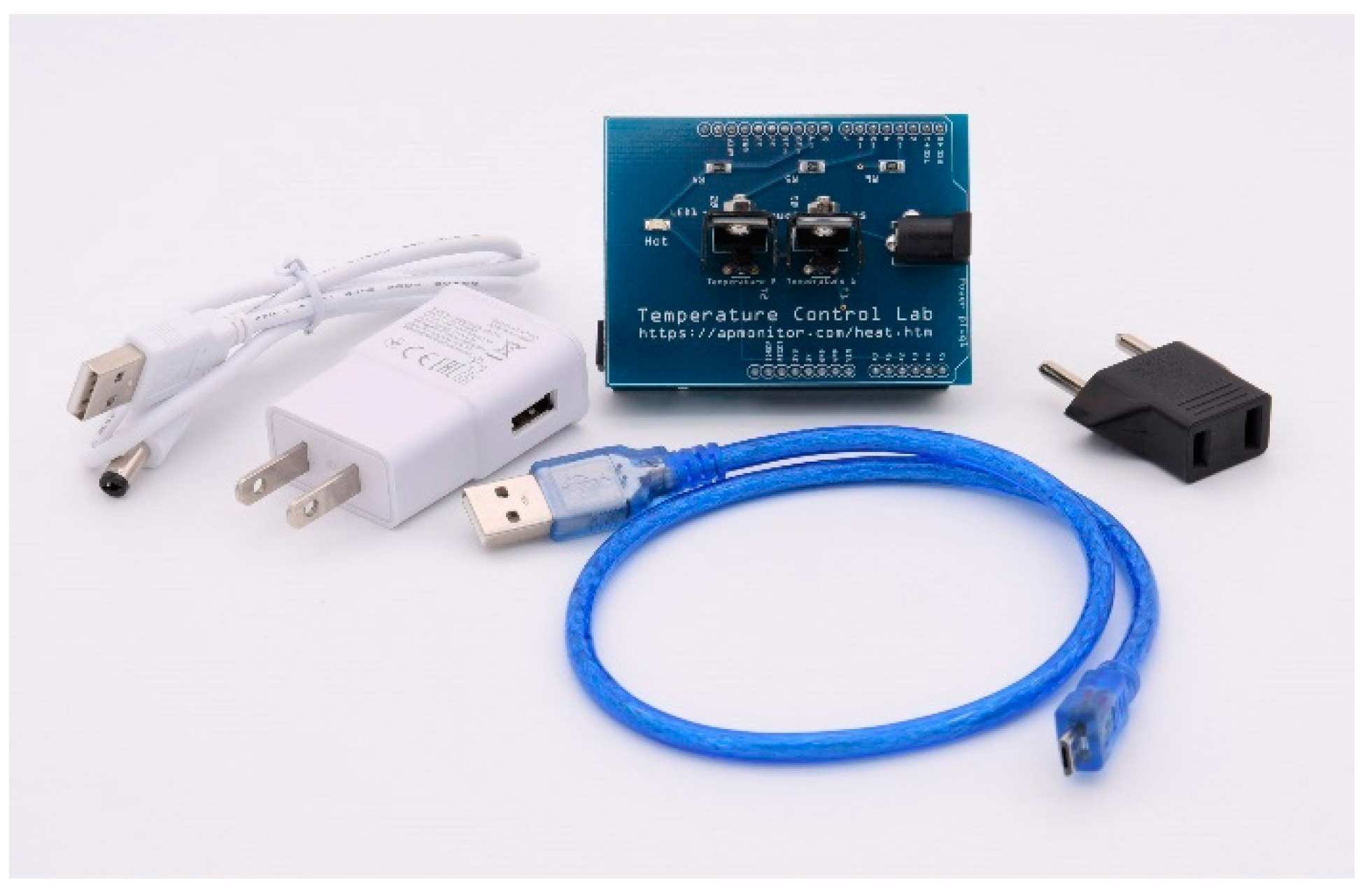
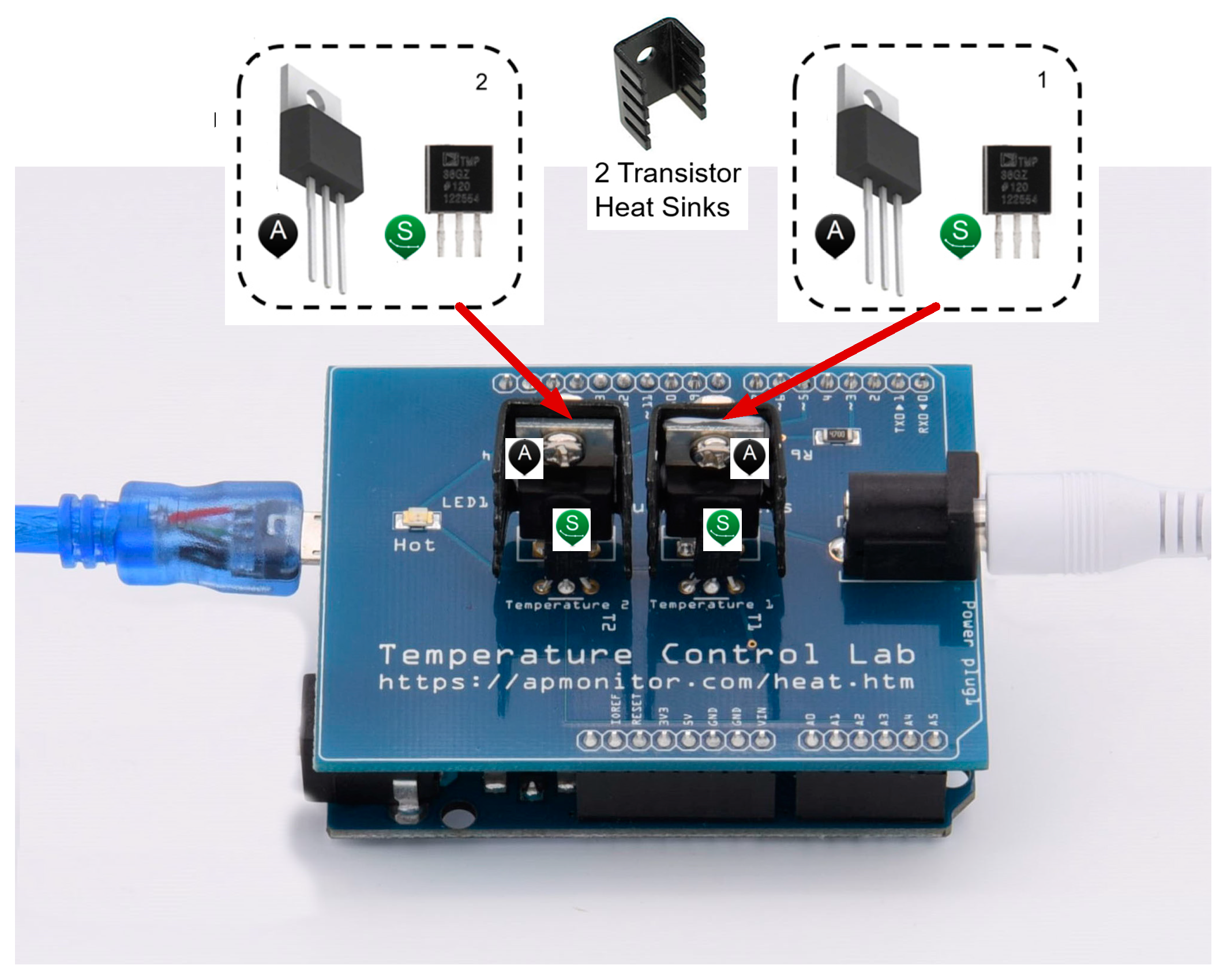
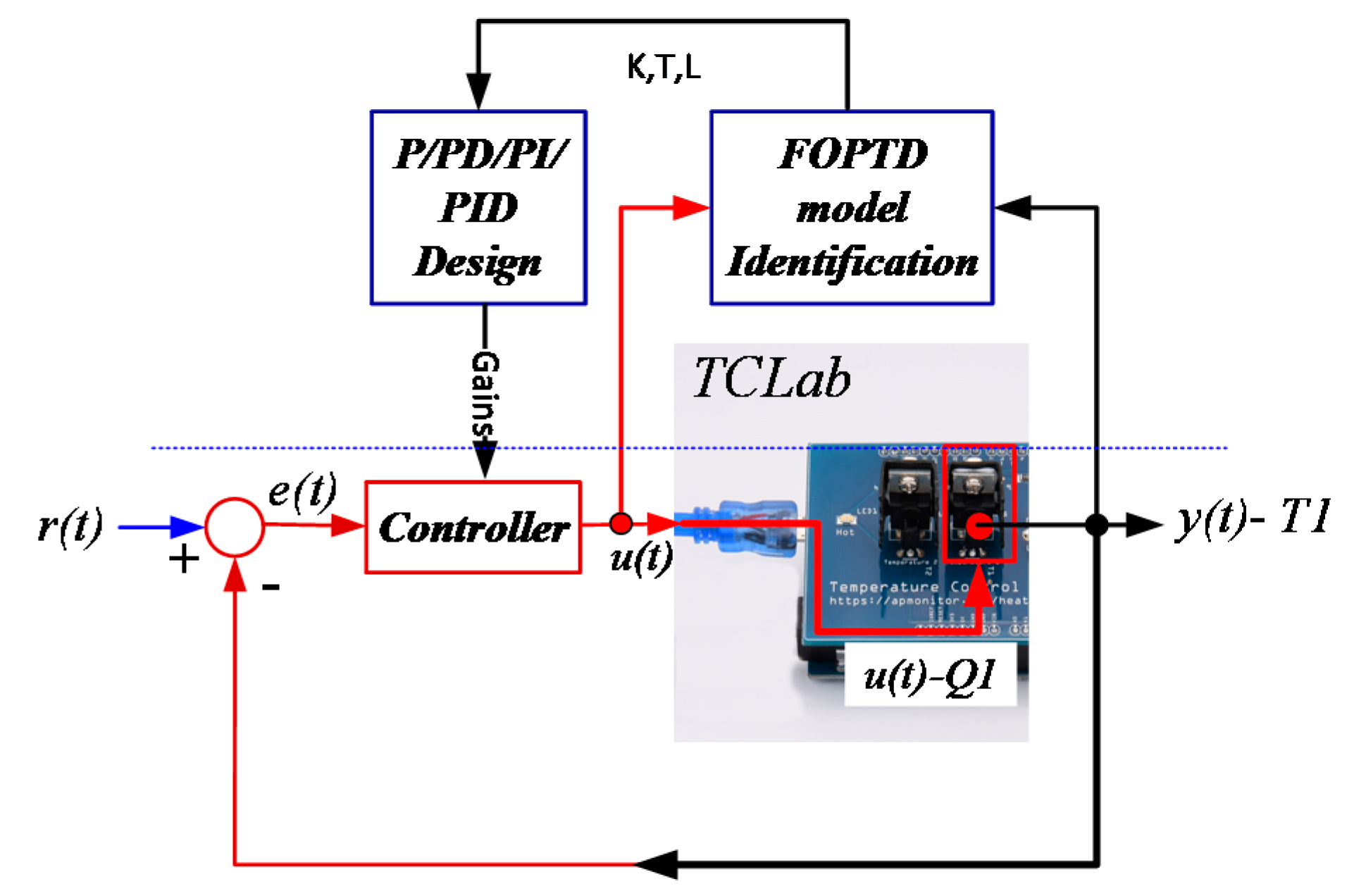
4. Temperature Control Laboratory (TCLab)

The Temperature Control Laboratory (TCLab) is an Arduino-based kit developed by [35]. It comes with the hardware set presented in Figure 3: An Arduino Leonardo; a Printed Circuit Board (PCB) with two transistors acting as heaters, two thermistors to sense the temperature in each transistor casing, an Light Emmiting Diode (LED) to indicate when the system is hot, and a connection socket to power the PCB components (see the white USB adapter shown in Figure 3); and finally, a Universal Serial Bus (USB) cable connects the Arduino to a computer (see the blue cable shown in Figure 3).
The TCLab is presented from another perspective in Figure 4. As it can be observed, the transistors (TIP31C) are the control system actuators and operate as temperature heaters (Q1 and Q2). Two TMP36 sensors measure the temperature in each transistor casing (T1 and T2). As it can also be observed from Figure 4, the two transistors are connected to heat sinks acting as heat dissipators. The sensors are glued to the transistor casings using a non-conductive epoxy containing a thermochromic paint. This paint changes color when the temperature rises above 37 °C. The TCLab can be programmed using MATLAB®/SIMULINK®, Python and GNU Octave, with a wide range of programs freely available in [22]. This study uses the MATLAB®/SIMULINK® connection. More information regarding TCLab can also be found in [35,36,37,38].

5. TCLab Results

Designing PID controllers with the proposed PSO technique involves (a) identifying a First-Order Plus Time Delay (FOPTD) model using an open-loop step response, (b) based on the obtained model in (a), another PSO algorithm is used to tune the PID controller. These two steps are illustrated in Figure 5 with the TCLab system.

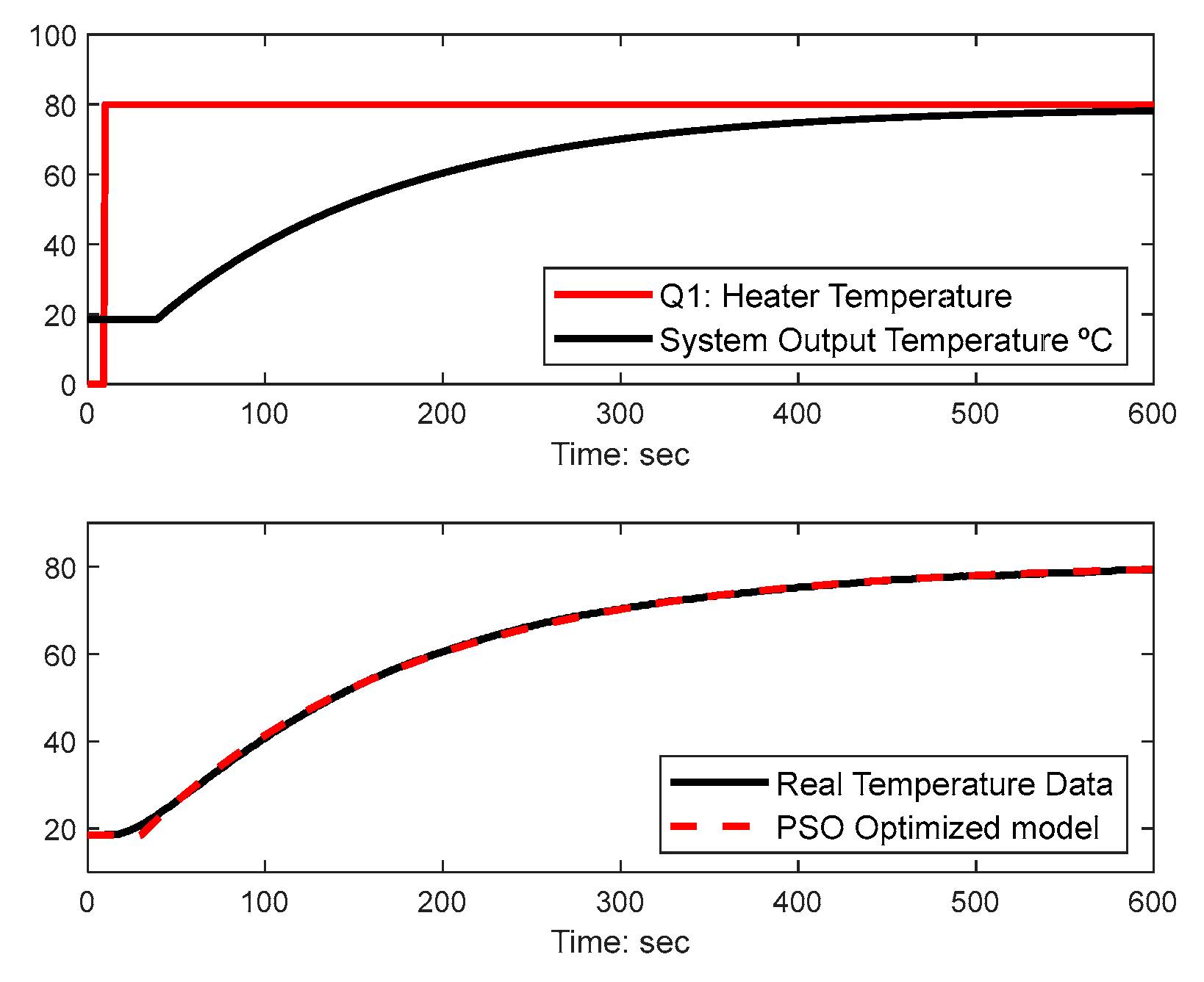
5.1. First-Order Plus Time Delay Model Identification

The first issue that must be addressed is to identify a dynamic model relating temperature measured in transistor 1 (T1) with the actuating heater signal (Q1). A FOPTD model was identified based on an open-loop step response using both the classical two-point and PSO optimization methods as proposed in [39,40]. The following PSO conditions were used in the model identification tests:
  • A swarm with size m = 40 particles.
  • Each simulation was run for 50 iterations.
  • The search intervals used for the controllers gains K, T, and L are: [0.1 3], [20 s 160 s], and [4 s 45 s], respectively. The FOPTD model parameters obtained with a classical step-response method (e.g., two-point method (see [28])) can be used to define the search interval.
  • The inertia weight was initial and final values were ωinit = 0.7 and ωfin = 0.4. These values were deemed appropriate with 50 iterations.
Figure 6 is a step response of the TCLab open-loop response. This figure top plot is a step applied to the system input (heater Q1) with amplitude ranging from 0–80% applied at instant t = 10 s. The bottom plot is the result obtained with a FOPTD model identified using a PSO. The model [30,40] is:
G p ( s ) = 0.78 1 + 152   s e 19.7 s

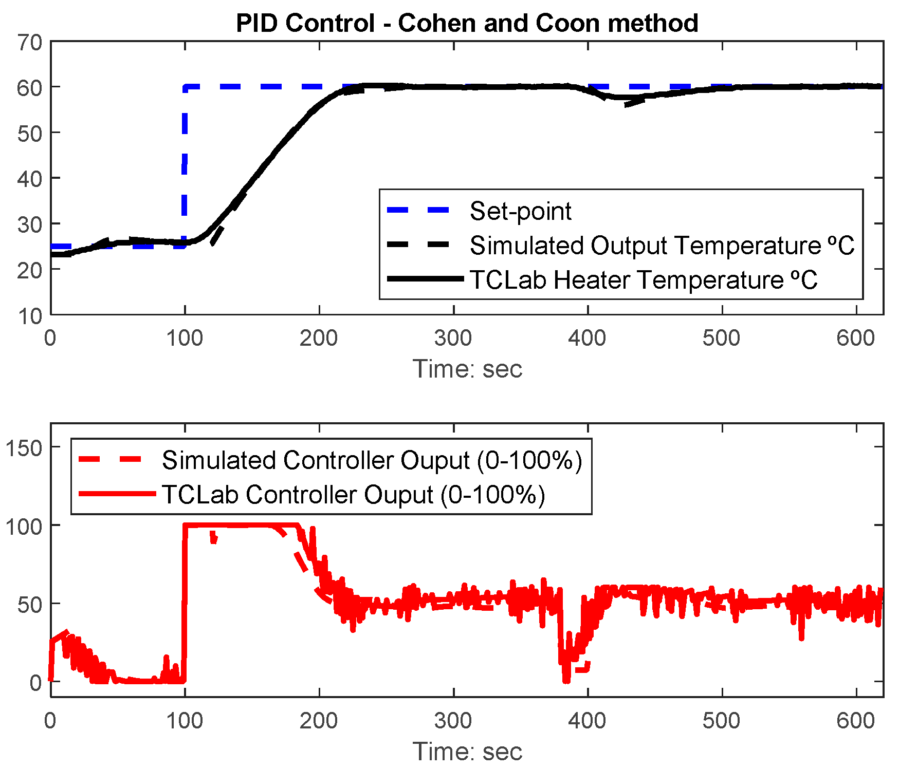
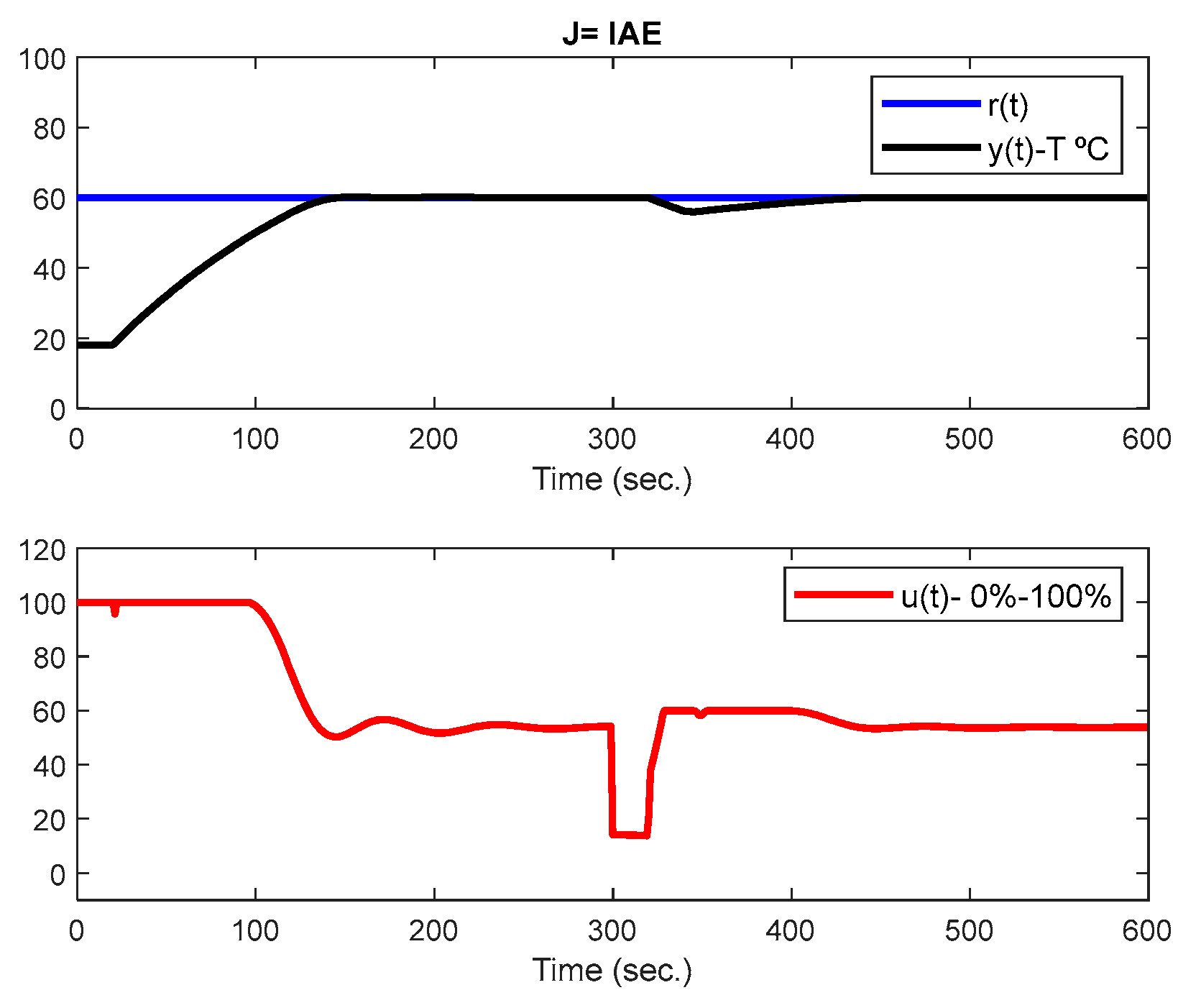
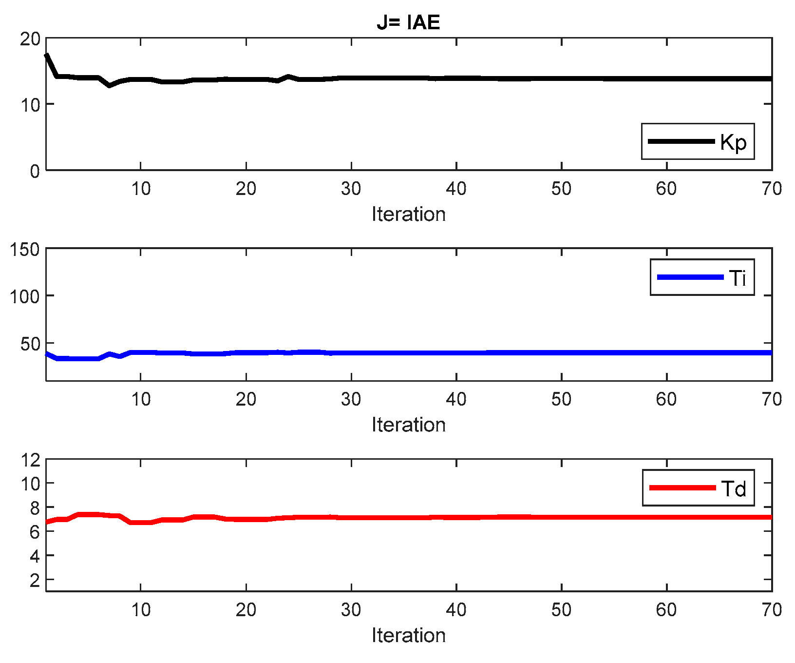
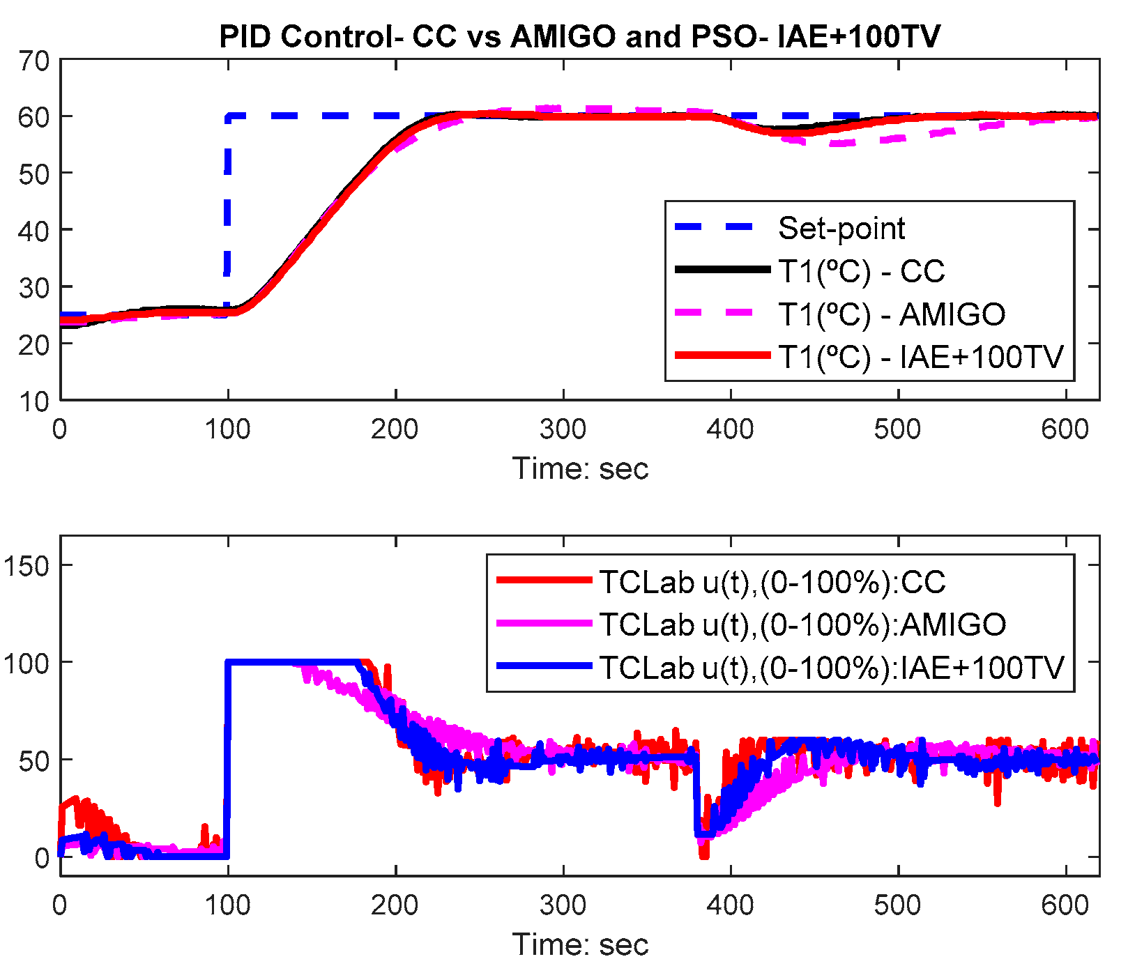
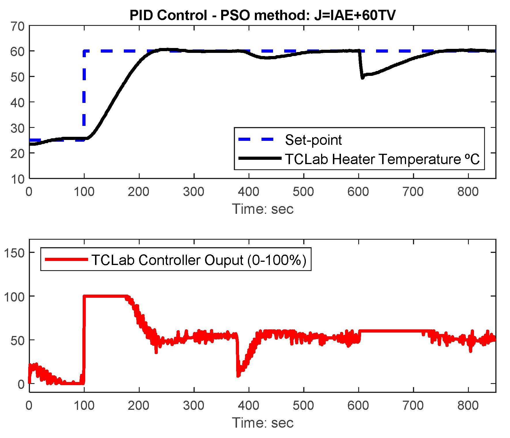
5.2. PID Controller Tuning

This section presents both simulation and TCLab results regarding the PID controller gains optimized with the PSO algorithm as depicted in the previous sections. The results are compared with the Cohen-Coon (CC) settings [43], as previously introduced in [39,40] and a more recent technique: AMIGO [5], which is well-known to achieve system robustness. For the sake of experiment replication, these two tuning rule methods for PID controllers are presented in Table 1.
Based on the FOPTD PSO model, PID controllers can be designed using several tuning methods. In [40], results were presented using the Cohen-Coon (CC) settings as these perform well for the TCLab. The results obtained with the CC PID settings Kp = 13.47, Ti = 45.99 s, and Td = 7.00 s are presented in Figure 7. This figure presents the overlapped results between the simulated and TCLab responses. A step input is applied to the system reference input at t = 0 s to define the TCLab transistor 1 set-point temperature at 25 °C and another one at t = 100 s increasing the set-point to 60 °C. A load disturbance with a magnitude of −40% is applied to the controller output at t = 380 s. Both the FOPTD model and the CC PID gains are used in the next section for comparison purposes with the other methods.
The PSO optimization simulations were carried out in MATLAB®/SIMULINK®. The PSO settings were defined for all the subsequent PID controller tuning simulations as follows:
  • A swarm with size m = 30 particles.
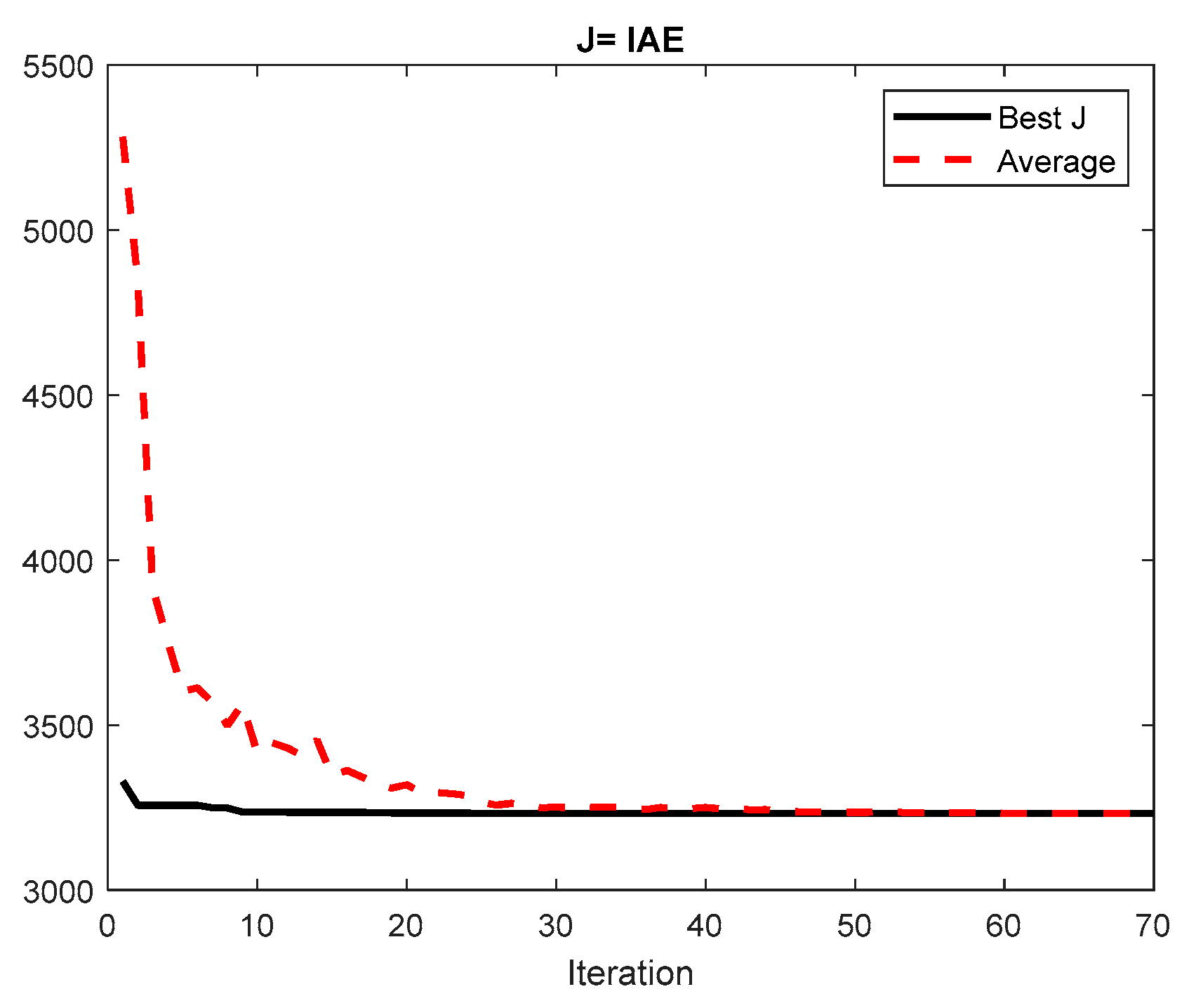
  • Each simulation was run for 70 iterations.
  • The search intervals used for the controller gains Kp, Ti, and Td are: [0.1 20], [10 s 150 s], and [1 s 12 s], respectively. The tuning gains obtained with classical tuning rules can be used (e.g., CC) to define the search interval. The interval used for the integral gain was widened to see if the PSO converged for slower TCLab control system responses.
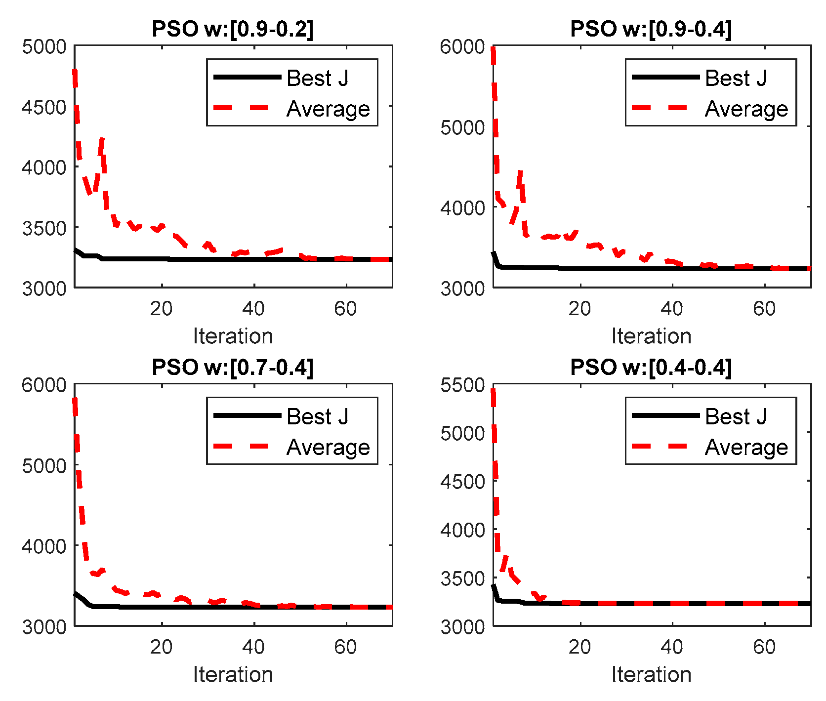
  • The inertia weight for initial and final values were ωinit = 0.7 and ωfin = 0.4. These values were deemed appropriate considering the number of iterations used, as it can be observed from Figure 8. In this figure, four different inertia weight intervals [ωinit, ωfin] were considered: (a) [0.9, 0.2], (b) [0.9, 0.4], [0.7, 0.4], and [0.4, 0.4].
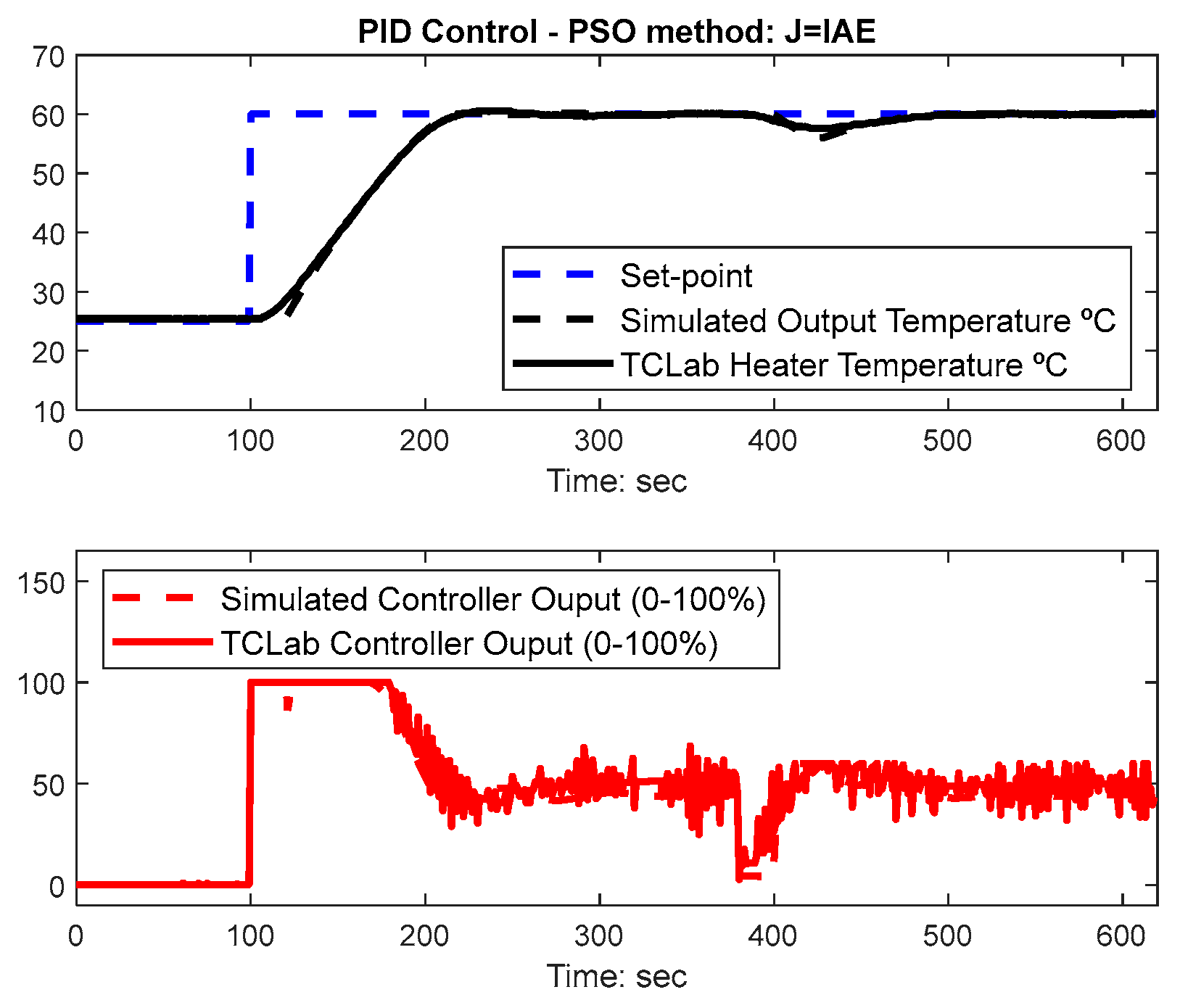
Note that the conditions used for conducting the PSO optimization PID tuning tests differ from the ones used to perform the FOPTD model identification, particularly in the swarm size and higher iteration number. The PSO convergence rate for the PID optimization was found to be slower than the FOPTD model identification case.
The optimizations consider a step response applied at the reference input at t = 0 s assuming an ambient temperature of 18 °C and a set-point of 60 °C. The simulation time was 600 s, and a load disturbance with amplitude −40% was applied at instant t = 300 s. The optimization test result considering just the minimization of IAE is presented in Figure 9, Figure 10 and Figure 11. In this case, the gains converged to the following values: Kp = 13.83, Ti = 39.54 s, and Td = 7.14 s. Figure 9 presents the SPT and LDR responses in the top plot and the control signal in the lower plot. As it can be observed, the system tracks well with no overshoot and with an acceptable load disturbance rejection.
Figure 10 shows the best PID gains evolution over 70 iterations. It is possible to observe from Figure 10 that the parameters converged to values are very close to the final ones by iteration 40. Figure 11 presents the evolution obtained with the best swarm cost value, IAE, and the average of the entire swarm particles cost function values. As observed, there is a convergence between the average and the best values in between iterations 40 and 50. These results clearly indicate that 70 iterations are an adequate stopping criterion, in this case.
After comparing the relative simulated values obtained for IAE and TV, the following cases were considered:
  • I: α = 1 and β = 0.
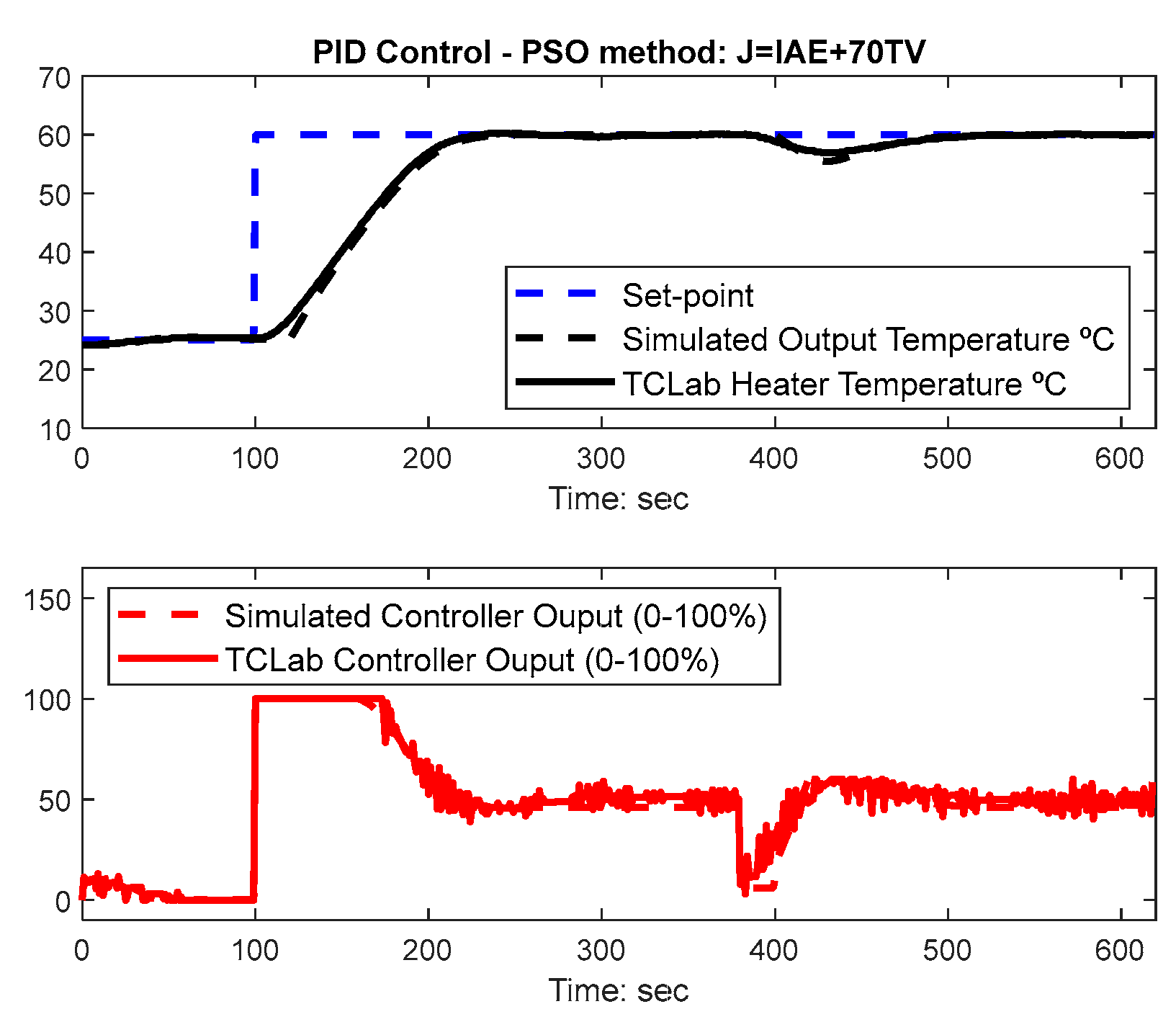
  • II: α = 1 and β = 70.
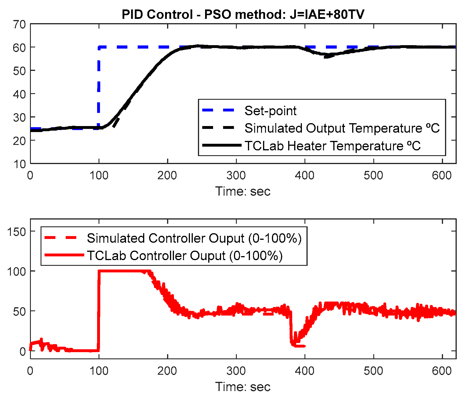
  • III: α = 1 and β = 80.
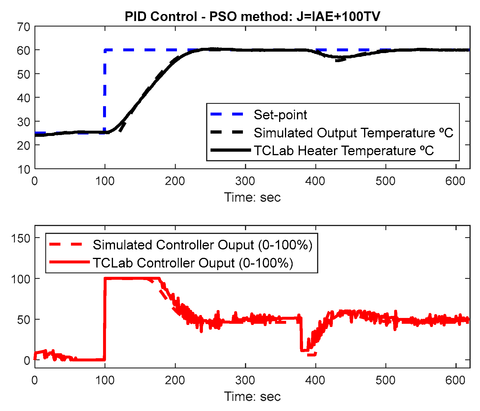
  • IV: α = 1 and β = 100.
Notice that this selection was done based on several tests performed on the TCLab. For cases with an additive compromise function, more relevance was given to TV over IAE. Before presenting the TCLab PSO results, a performance comparison with another swarm optimization algorithm, the original Grey Wolf Optimization (GWO) [18], is presented. The GWO was compared with the classical PSO in a benchmark test suit when it was proposed [18]. The GWO swarm size, number of iterations, and PID controller gains interval are the same as the ones used for the PSO. The GWO algorithm uses a heuristic parameter, represented by a [18] responsible for the tradeoff swarm exploration and exploitation. The GWO parameter a is a linearly decreasing vector from amax = 2 to amin = 0 through the evolutionary process. The simulation results are presented in Table 2 for cases I and II. The best controller gains from an 11 run set converged to very similar IAE and TV values. This indicates that with the appropriate settings the classical PSO performs, as well as the classical GWO for this control case study. More information regarding a comparison between PSO, GWO, and GSA for the PID control is reported in [19].
A compilation of the results with the classic tuning rules and PSO optimization is presented in Table 3. The best PSO gains presented in Table 2 are replicated in Table 3 for comparison. Note also that as the TCLab tests were performed in different day periods, the initial starting ambient temperature varies slightly from test to test. To see if this influenced the results analysis, the IAE and TV values considered only the period [95–620 s] (see Table 4). This interval starting point corresponds to 5 s prior to the second step change at t = 100 s where all the temperature steady-state values are approximately equal to 25 °C.
The results obtained with the AMIGO PID settings: Kp = 4.69, Ti = 72.94 s, and Td = 9.48 s are presented in Figure 12. As it can be observed, the response presents a pronounced overshoot and worse load rejection disturbance compared with the CC response. The TV value obtained with the AMIGO settings is clearly better than the one obtained with CC (see Table 3 and Table 4).
The results obtained for PSO with just the ITAE minimization criterion (PSO-I) are presented in Figure 13. As it can be seen from Table 3 and Table 4, only minimizing the IAE results in the best possible IAE value and worse TV than with the CC and AMIGO methods.
The results obtained by using cost functions (8) with α = 1 and β = 70 (PSO-II), α = 1 and β = 80 (PSO-III), α = 1 and β = 100 (PSO-IV), are presented respectively in Figure 14, Figure 15 and Figure 16.
Observing the values obtained with the four PSO cases, the IAE value increases as expected. With the increase of the TV factor, β in the cost function, the corresponding TV value decreases. Depending on the TV requirements, it is possible to obtain better results for both IAE and TV compared with the CC and AMIGO tuning rules, as expected.
Figure 17 presents the overlap responses obtained with the TCLab regarding the following methods: CC, AMIGO, and PSO-IV. As it can be observed from the tracking response in the top plot, CC gains perform slightly better than the PSO-IV gains and these two are much better than AMIGO. However, regarding the control signals in the bottom plot, the optimized PSO gains result in a less aggressive and less irregular control signal variation than CC and AMIGO.
The results also consider an output disturbance applied at instant t = 600 s, as presented in Figure 18. In this case, the disturbance was caused by blowing with a straw near the transistor 1 for 5 s, to decrease the temperature. As it can be observed, the response also tracks well from the output disturbance.

6. Conclusions

The design of Proportional, Integral, and Derivative controllers (PID) using a technique based on the particle swarm optimization algorithm is presented in this work. Classical PID tuning rules are dependent of the system dynamics and PID controller structure. Moreover, the PID settings in most methods differ according to the specific control design objective (e.g., set-point tracking or load disturbance rejection). The proposed PSO-based PID controller optimization technique holds the following characteristics which are of great practical interest: (a) To be easily implemented in digital industrial computers/microcontrollers; (b) to cope simultaneously with several control design criteria; (c) can be applied to control systems independently of system dynamics; and (d) rely in a reduced number of heuristic parameters, which can be easily adjusted for control purposes.
The merits of the proposed design technique lie within:
  • The use of an additive compromise cost function involving the minimization of two performance criteria: The Integral Absolute Error (IAE) and the Total Variation (TV). By using a simple compromise cost function, the proposed PID controller design technique simultaneously considers the following major control design criteria: Set-point tracking, load disturbance rejection, and control signal variation.
  • By using the proposed cost function, it was shown that it is quite simple to select the PSO heuristic parameters with a special emphasis on the inertia weight decay.
  • The PSO was used to both perform the TCLab system identification as well as PID controller tuning. In both optimization problems, the proposed technique blends quite well with classical design techniques. One of the problems with the use of optimization algorithms in practical problems is to define appropriate decision variable search intervals. The identification of a first-order plus time delay model with the PSO technique uses the two-point step response method [39,40] to define the model parameter search space. The Cohen-Coon PID controller tuning rules were used to define the controller gain search space.
  • The PSO results for the specific TCLab control case performs as well as a much more recently introduced metaheuristic: The grey wolf optimization.
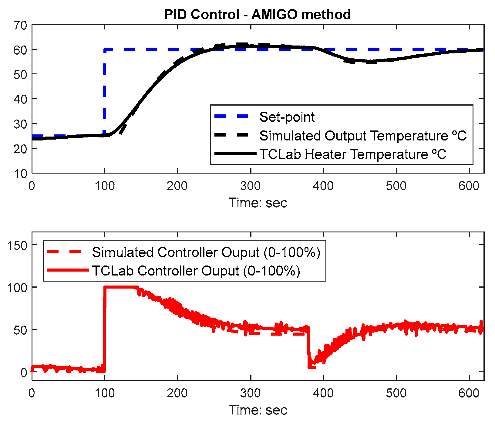
  • The proposed technique was tested with an Arduino Temperature Control Laboratory (TCLab) and compared with well-established PID tuning methods. Both the simulation as well as physical TCLab results were presented to provide evidence of improved control performance. The results show a good agreement between the simulation and measured results to validate the dynamic model identified with PSO.
  • The TCLab Arduino kit was introduced as a simple to use portable laboratory to test simulation results obtained with the proposed PSO-based technique. The same device has great potential to test other optimization and artificial intelligence-based techniques.

Author Contributions

P.B.d.M.O. was involved in the proposed technique conceptualization, validation, TCLab software, and physical experiments; J.D.H. was involved in the TCLab Arduino kit experiment methodology, software, and prosed technique results analysis; E.J.S.P. was involved in the proposed technique validation. All authors were involved in the writing of the original draft preparation, review, and editing. All authors have read and agreed to the published version of the manuscript.

Funding

This research received no external funding.

Conflicts of Interest

The authors declare no conflict of interest.

References

  1. Starr, K.; Bauer, M.; Horch, A. An Industry Sponsored Video Course for Control Engineering Practitioners. IFAC PapersOnLine 2015, 48, 59–64. [Google Scholar] [CrossRef]
  2. PID-18. In Proceedings of the 3rd IFAC Conference on Advances in Proportional-Integral-Derivative Control, Ghent, Belgium, 9–11 May 2018; Available online: https://0-www-sciencedirect-com.brum.beds.ac.uk/journal/ifac-papersonline (accessed on 20 October 2020).
  3. Ziegler, J.G.; Nichols, N.B. Optimum settings for automatic controllers. Trans. ASME 1942, 31, 759–768. [Google Scholar] [CrossRef]
  4. Peng, Y.; Vrančić, D.; Hanus, R. Anti-windup, bumpless, and conditioned transfer techniques for PID controllers. IEEE Control Syst. Mag. 1996, 16, 4. [Google Scholar] [CrossRef]
  5. Åström, K.J.; Hägglund, T. Advanced PID Control; ISA: Research Triangle Park, NC, USA, 2006; ISBN 1-55617-942-1. [Google Scholar]
  6. Seborg, D.; Edgar, T.F.; Mellichamp, D.A.; Doyle, F.J., III. Process Dynamics and Control, 4th ed.; Wiley: Hoboken, NJ, USA, 2017; ISBN 978-1-119-28591-5. [Google Scholar]
  7. Visioli, A.; Vilanova, R. PID Control in the Third Millennium: Lessons Learned and New Approaches; Springer: Berlin/Heidelberg, Germany, 2012; ISBN 978-1-4471-2424-5. [Google Scholar]
  8. Rossiter, A.; Zakova, K.; Huba, M.; Serbezov, A.; Visioli, A. A First Course in Feedback, Dynamics and Control: Findings from 2019 Online Survey of the International Control Community. In Proceedings of the IFAC-2020 World Congress, Berlin, Germany, 11–17 July 2020. [Google Scholar]
  9. Holland, J.H. Adaptation in Natural and Artificial Systems; The University of Michigan Press: Ann Arbor, MI, USA, 1975. [Google Scholar]
  10. Dorigo, M.; Maniezzo, V.; Colorni, A. Ant system: Optimization by a colony of cooperating agents. IEEE Trans. Syst. Man Cybern. 1996, 26, 29–41. [Google Scholar] [CrossRef] [Green Version]
  11. Koza, J.R. Genetic Programming: A Paradigm for Breeding Populations of Computers Programs to Solve Problems; Technical Report STAN-CS-90-1314; Stanford University: Stanford, CA, USA, 1990. [Google Scholar]
  12. Storn, R.; Price, K.V. Differential Evolution—A Simple and Efficient Adaptive Scheme for Global Optimization over Continuous Spaces. J. Global Optim. 1997, 11, 341–359. [Google Scholar] [CrossRef]
  13. Kennedy, J.; Eberhart, R.C. Particle swarm optimization. In Proceedings of the International Conference on Neural Networks, Perth, WA, Australia, 27 November–1 December 1995; pp. 1942–1948. [Google Scholar]
  14. Yang, X.-S.; Deb, S. Cuckoo Search via Lévy Flights. In Proceedings of the World Congress on Nature & Biologically Inspired Computing (NaBIC), Coimbatore, India, 8–10 February 2009; pp. 210–214. [Google Scholar]
  15. Yang, X.-S. Firefly Algorithm, Lévy Flights and Global Optimization. In Research and Development in Intelligent Systems XXVI; Bramer, M., Ellis, R., Petridis, M., Eds.; Springer: London, UK, 2010. [Google Scholar] [CrossRef]
  16. Krishnanand, K.N.; Ghose, D. Glowworm swarm based optimization algorithm for multimodal functions with collective robotics applications. Multiagent Grid Syst. Int. J. 2006, 2, 209–222. [Google Scholar] [CrossRef] [Green Version]
  17. Rashedi, E.; Nezamabadi-Pour, H.; Saryazdi, S. GSA: A Gravitational Search Algorithm. Inf. Sci. 2009, 179, 2232–2248. [Google Scholar] [CrossRef]
  18. Seyedali, M.; Mohammad, S.M.; Lewis, A. Grey wolf optimizer. Adv. Eng. Softw. 2014, 69, 46–61. [Google Scholar]
  19. Moura Oliveira, P.B.; Vrancic, D.E. Grey Wolf, Gravitational Search and Particle Swarm Optimizers: A Comparison for PID Controller Design. In CONTROLO 2016; Lecture Notes in Electrical Engineering; Springer: Guimarães, Portugal, 2016; Volume 402, pp. 239–249. [Google Scholar] [CrossRef]
  20. De Moura Oliveira, P.B.; Freire, H.; Solteiro Pires, E.J. Grey Wolf Optimization for PID Controller Design with Prescribed Robustness Margins. Soft Comput. 2016, 20, 4243–4255. [Google Scholar] [CrossRef]
  21. Rathore, N.S.; Singh, V.P.; Kumar, B. Controller design for Doha water treatment plant using grey wolf optimization. J. Intell. Fuzzy Syst. 2018, 35, 5329–5336. [Google Scholar] [CrossRef]
  22. Gupta, S.; Singh, V.P.; Singh, S.P.; Prakash, T.; Rathore, N.S. Elephant herding optimization based PID controller tuning. Int. J. Adv. Technol. Eng. Explor. 2016, 3, 194. [Google Scholar] [CrossRef]
  23. Jones, A.H.; De Moura Oliveira, P.B. Genetic Auto-Tuning of PID Controllers. In Proceedings of the First IEE Conference on Genetic Algorithms in Engineering Systems: Innovations and Applications (GALESIA’95), Sheffield, UK, 12–14 September 1995; Volume 414, pp. 141–145. [Google Scholar]
  24. Fleming, P.J.; Purshouse, R.C. Evolutionary algorithms in control systems engineering: A survey. Control Eng. Pract. 2002, 10, 1223–1241. [Google Scholar] [CrossRef]
  25. Coelho, P.C.; De Moura Oliveira, P.B.; Boaventura Cunha, J. Greenhouse Air Temperature Control using the Particle Swarm Optimisation Algorithm. Comput. Electron. Agric. 2005, 49, 330–344. [Google Scholar] [CrossRef] [Green Version]
  26. Moura Oliveira, P.B.; Solteiro Pires, E.J.; Boaventura Cunha, J.; Pinho, T.M. Review of Nature and Biologically Inspired Metaheuristics for Greenhouse Environment Control. Trans. Inst. Meas. Control 2020, 42, 2338–2358. [Google Scholar] [CrossRef]
  27. Fan Shu-Kai, S.; Zahara, E. A hybrid simplex search and particle swarm optimization for unconstrained optimization. Eur. J. Oper. Res. 2007, 181, 527–548. [Google Scholar]
  28. Fan, S.-K.S.; Jen, C.-H. An Enhanced Partial Search to Particle Swarm Optimization for Unconstrained Optimization. Mathematics 2019, 7, 357. [Google Scholar] [CrossRef] [Green Version]
  29. Irigoyen, E.; Larzabal, E.; Priego, R. Low-cost platforms used in Control Education: An educational case stud. In Proceedings of the 10th IFAC Symposium Advances in Control Education, Sheffield, UK, 28–30 August 2013. [Google Scholar]
  30. Reguera, V.; García, D.; Domínguez, M.; Prada, M.A.; Alonso, S. A low-cost open source hardware in control education. Case study: Arduino-Feedback MS-150. IFAC PapersOnLine 2015, 48, 117–122. [Google Scholar] [CrossRef]
  31. McLoone, S.C.; Maloco, J. A Cost-effective Hardware-based Laboratory Solution for Demonstrating PID Control. In Proceedings of the UKACC 11th International Conference on Control (CONTROL), Belfast, UK, 31 August–2 September 2016. [Google Scholar]
  32. Prima, E.C.; Saeful, K.; Utarib, S.; Ramdanib, R.; Putri, E.R.; Darmawatib, S.M. Heat Transfer Lab Kit using Temperature Sensor based Arduino TM for Educational Purpose. Procedia Eng. 2017, 170, 536–540. [Google Scholar] [CrossRef]
  33. Rossiter, J.A.; Pope, S.A.; Jones, B.L.; Hedengren, J.D. Evaluation and demonstration of take-home laboratory kit, Invited Session: Demonstration and poster session. In Proceedings of the 12th IFAC Symposium on Advances in Control Education, Philadelphia, PA, USA, 7–9 July 2019. [Google Scholar]
  34. Juchem, J.; Chevalier, A.; Dekemele, K.; Loccu, M. Active learning in control education: A pocket-size PI(D) setup. In Proceedings of the IFAC-2020 World Congress, Berlin, Germany, 11–17 July 2020. [Google Scholar]
  35. Hedengren, J.D. Temperature Control Lab Kit. Available online: https://apmonitor.com/heat.htm (accessed on 20 September 2020).
  36. Hedengren, J.D.; Martin, R.A.; Kantor, J.C.; Reuel, N. Temperature Control Lab for Dynamics and Control. In Proceedings of the AIChE Annual Meeting, Orlando, FL, USA, 10–15 November 2019. [Google Scholar]
  37. Park, J.; Patterson, C.; Kelly, J.; Hedengren, J.D. Closed-Loop PID Re-Tuning in a Digital Twin by Re-Playing Past Setpoint and Load Disturbance Data. In Proceedings of the AIChE Spring Meeting, New Orleans, LA, USA, 31 March–4 April 2019. [Google Scholar]
  38. Park, J.; Martin, R.A.; Kelly, J.D.; Hedengren, J.D. Benchmark Temperature Microcontroller for Process Dynamics and Control. J. Comp. Chem. Eng. 2020, 135, 6. [Google Scholar] [CrossRef]
  39. Moura Oliveira, P.B.; Hedengren, J.D. An APMonitor Temperature Lab PID Control Experiment for Undergraduate Students. In Proceedings of the 24th IEEE International Conference on Emerging Technologies and Factory Automation (ETFA), Zaragoza, Spain, 10–13 September 2019; pp. 790–797. [Google Scholar]
  40. Moura Oliveira, P.B.; Hedengren, J.D.; Rossiter, J.A. Introducing Digital Controllers to Undergraduate Students using the TCLab Arduino Kit. In Proceedings of the IFAC-2020 World Congress, Berlin, Germany, 11–17 July 2020. [Google Scholar]
  41. Freire, H.; Moura Oliveira, P.B.; Pires, E.J. From Single to Many-objective PID Controller Design using Particle Swarm Optimization. Int. J. Control Autom. Syst. 2017, 15, 918–932. [Google Scholar] [CrossRef]
  42. Bansal, J.C.; Singh, P.K.; Saraswat, M.; Verma, A.; Jadon, S.S.; Abraham, A. Inertia Weight Strategies in Particle Swarm Optimization. In Proceedings of the IEEE Third World Congress on Nature and Biologically Inspired Computing, Salamanca, Spain, 19–21 October 2011; pp. 633–640. [Google Scholar]
  43. Cohen, G.H.; Coon, G.A. Theoretical consideration of retarded control. Trans. ASME 1953, 75, 827–834. [Google Scholar]
Figure 1. General closed-loop control system block diagram.
Algorithms 13 00315 g001
Figure 2. Particle swarm optimization algorithm: Position, velocity, and personal and global best variables data representation.
Algorithms 13 00315 g002
Figure 3. Temperature control lab (TCLab) hardware set.
Algorithms 13 00315 g003
Figure 4. TCLab with power and USB connections. Actuators and sensors outlined with letters A and S, respectively.
Algorithms 13 00315 g004
Figure 5. TCLab system identification and controller tuning approach.
Algorithms 13 00315 g005
Figure 6. TCLab open-loop step response (top plot) and particle swarm optimization (PSO) model step response overlapped with the real TCLab data (bottom plot).
Algorithms 13 00315 g006
Figure 7. Simulated and TCLab responses using Cohen-Coon settings.
Algorithms 13 00315 g007
Figure 8. PSO evolution of the best integral absolute error (IAE) values and average swarm IAE values corresponding to four different inertia weight variation settings.
Algorithms 13 00315 g008
Figure 9. TCLab set-point tracking (SPT) and disturbance rejection (DR) simulated responses with a PID controller optimized with the PSO algorithm (J = IAE).
Algorithms 13 00315 g009
Figure 10. PSO evolution of the PID controller gains resulting in the final values used in the system response of Figure 9.
Algorithms 13 00315 g010
Figure 11. PSO evolution of the best IAE value and average swarm IAE values corresponding to the test in Figure 9 and Figure 10.
Algorithms 13 00315 g011
Figure 12. Simulated and TCLab responses using AMIGO settings.
Algorithms 13 00315 g012
Figure 13. Simulated and TCLab responses using PSO, case I (J = IAE).
Algorithms 13 00315 g013
Figure 14. Simulated and TCLab responses using PSO, case II (J = IAE + 70 TV).
Algorithms 13 00315 g014
Figure 15. Simulated and TCLab responses using PSO, case III (J = IAE + 80 TV).
Algorithms 13 00315 g015
Figure 16. Simulated and TCLab responses using PSO, case IV (J = IAE + 100 TV).
Algorithms 13 00315 g016
Figure 17. TCLab responses overlapping the responses for Cohen-Coon (CC), AMIGO, and PSO, case IV (J = IAE + 100 TV).
Algorithms 13 00315 g017
Figure 18. TCLab responses using PSO (J = IAE + 60 TV). Output disturbance considered at t ≅ 600 s.
Algorithms 13 00315 g018
Table 1. Cohen-Coon [32] and AMIGO [5] proportional, integral, and derivative (PID) tuning rules.
MethodKpTiTd
Cohen-Coon 1 K T L ( 4 3 + L 4 T ) L 32 + 6 L T 13 + 8 L T L 4 11 + 2 L T
AMIGO ( 1 K ) ( 0.2 + 0.45 T L ) ( 0.4 L + 0.8 T L + 0.1 T ) L 0.5 LT 0.3 L + T
Table 2. TCLab simulation results obtained with the PSO and grey wolf optimization (GWO) algorithms. The best results are represented in bold.
MethodKpTi (s)Td (s)IAETV
PSO-I13.8339.547.144442.02843.8
GWO-I13.8239.497.134441.82843.8
PSO-II9.6449.295.703831.42444.7
GWO-II10.4047.556.083834.42429.0
PSO-III10.3647.706.054438.52921.4
GWO-III10.2347.975.974437.52924.8
PSO-IV9.5349.695.654430.72936.6
GWO-IV10.1748.145.934436.82927.0
Table 3. TCLab physical results obtained for the several methods considering the entire test time. The best results are represented in bold.
MethodKpTi (s)Td (s)IAETV
CC13.4745.997.002389.42962.2
AMIGO4.6972.969.483004.91972.3
PSO-I13.8339.547.142273.63600.4
PSO-II9.6449.295.702298.52216.7
PSO-III10.3647.706.052392.52164.8
PSO-IV9.5349.695.652482.71888.4
Table 4. TCLab physical results obtained for the several methods considering the time interval [95–620 s]. The best results are represented in bold.
MethodIAETV
CC2300.92647.9
AMIGO2953.51860.6
PSO-I2235.83594.1
PSO-II2259.92102.6
PSO-III2351.12065.8
PSO-IV2442.01788.8
Publisher’s Note: MDPI stays neutral with regard to jurisdictional claims in published maps and institutional affiliations.

