Evaluation of Agricultural Investment Climate in CEE Countries: The Application of Back Propagation Neural Network

Abstract

Evaluation of agricultural investment climate has essential reference value for site selection, operation and risk management of agricultural outward foreign direct investment projects. This study builds a back propagation neural network-based agricultural investment climate evaluation model, which has 22 indicators of four subsystems that take political climate, economic climate, social climate, and technological climate as the input vector, and agricultural investment climate rating as the output vector, to evaluate the agricultural investment climate in 16 Central and Eastern European (CEE) countries. The overall spatial distribution characteristics demonstrate that the best agricultural investment climate is in the three Baltic countries, followed by the Visegrad Group and Slovenia sector, and then the Balkan littoral countries. The findings may provide insights for entrepreneurs who aim to invest in agriculture abroad and contribute to the improvement of these countries’ investment climate.

1. Introduction

With the highlight of a few questions, such as the acceleration of the economic globalization process and increasing agricultural investment pace, conducting a full and systematic analysis of the host country’s agricultural climate has become the first and foremost issue in the process of outbound investment [1]. The concept of “investment climate” was first proposed in 1968, which marked the rise of investment climate research to a theoretical level. Since then, relevant research has focused on applied evaluation, but few specific studies have been conducted on agricultural investment climate alone. World Bank defined investment climate as a set of location-specific components forming the openings and motivating climate for firms to grow [2]. According to relevant literature, it has been demonstrated that the investment climate plays a vital role in the growth of both economy and enterprise [3,4,5,6,7]. Litvak and Banting analyzed the agricultural investment climate components in terms of political stability, legal barriers, market opportunities, economic development achievements, physical barriers, cultural integration, geographical and cultural gaps, and constructed a comprehensive evaluation index system [8]. Hardaker divided the agricultural risk index system into seven significant risks: institutional risk, production risk, market risk, financing risk, currency risk, legal risk, and personal risk [9].

Relevant literature shows that the industrial climate’s systematic analysis of the host country is mostly based on the PEST theory proposed by Johnson and Scholes, which mainly focuses on the external climate. The macro-climate refers to the various macro factors that may affect the regular operation of an industry or an enterprise, which are generally considered from four aspects: political (P), economic (E), social (S), and technological (T) [10,11,12]. The macro influencing factors are transferred with different targets, which need to be “customized”. The literature also provides a consensus that a favorable investment climate could benefit an enterprise’s growth. On the contrary, an adverse investment climate endangers the enterprise’s growth [13,14]. Due to the influence of intricate geopolitical patterns of CEE countries [15], agricultural enterprises may encounter unexpected compound risks in the process of direct investment in this area. Therefore, this theory is conducive for enterprises to understand the nature of the outbound climate and evaluate the sustainability of CEE countries’ agricultural investment climate.

Over an extended period, due to the uncertainty and ambiguity of regional investment climatical factors, scholars mainly adopt the principal component analysis method [16,17,18], fuzzy comprehensive evaluation method [19,20,21], gray correlation [22], and other methods to research on investment climate evaluation [23,24,25]. However, the above methods have two major common problems: Firstly, these methods are static models, which obtain investment indexes by collecting and extracting a large amount of data and relevant information. Therefore, the model itself lacks the adaptability of information and memory functions. When the factors affecting the investment climate change, such methods are difficult to function, so their effectiveness is significantly reduced. In order to improve the evaluation’s accuracy, the variables or parameters need to be adjusted based on variable data or information, or even need to reconstruct the evaluation model. On the other hand, this type of approach is highly subjective. The method is primarily influenced by the experts’ knowledge or investors’ subjective experience. The global investment climate is ever-changing, and the influencing factors are involved, making it challenging to ensure the accuracy and objectivity of every subjective decision. The rating experts’ different backgrounds may easily lead to disagreement, resulting in increased time and hiring costs, which also lead to certain flaws in the scientific and objective principles of the indicator system. Since the evaluation system’s weighting has a more significant impact on the final rating results, even if the results are in line with subjective expectations, it is prone to more significant distortion [26].

In summary, only a few scholars have researched on the investment climate of agriculture, and even less use of neural network analysis methods. At present, there is an urgent need to integrate a large number of information resources for agricultural investment climate evaluation and to establish an artificial mechanism that can transform the subjective feelings of experts into an internal flexible decision-making system, on the basis of which to build a general evaluation decision-making model. Therefore, this paper attempts to apply the back propagation (BP) neural network technique to construct an agricultural investment climate evaluation model for CEE countries. This paper addresses the lack of specific consideration of the factor endowments of the agricultural investment environment in existing academic research. It explores the development of the agricultural environment in CEE countries in order to fill in the gaps and deficiencies related to the combined analysis of neural network and the agricultural investment environment. The practical significance of this paper lies in the fact that agricultural resources and conditions in CEE countries are characterized by diversity and differentiation, which brings certain challenges for agricultural enterprises to invest. Against this background, this paper provides an in-depth analysis of the agricultural investment climate in CEE countries, which will help enterprises explore potential opportunities for agricultural investment in different host countries and provide external environment analysis and information support for enterprises to make full use of international resources and participate in international market competition.

2. Methods

2.1. Back Propagation Neural Network

2.1.1. Back Propagation Neural Network Structure

Artificial neural network (ANN) is an up-and-coming network algorithm tool hinging on self-learning, which means it does not require a human to set the weights and automatically adjust the weights through deep learning. ANN is related to a signal processing system and information composed of a massive number of called neurons that stimulate the biological nervous system in a program. These neurons connect to each other through direct connections called synapses, allowing distributed parallel processing. The main characteristic of ANN is its adaptability, which could learn and establish accurate and complex relationships among various numerical variables without the need for any pre-defined models [27]. ANN is often used in systems where no mathematical model exists or is precise enough to represent the phenomenon [28,29,30,31].

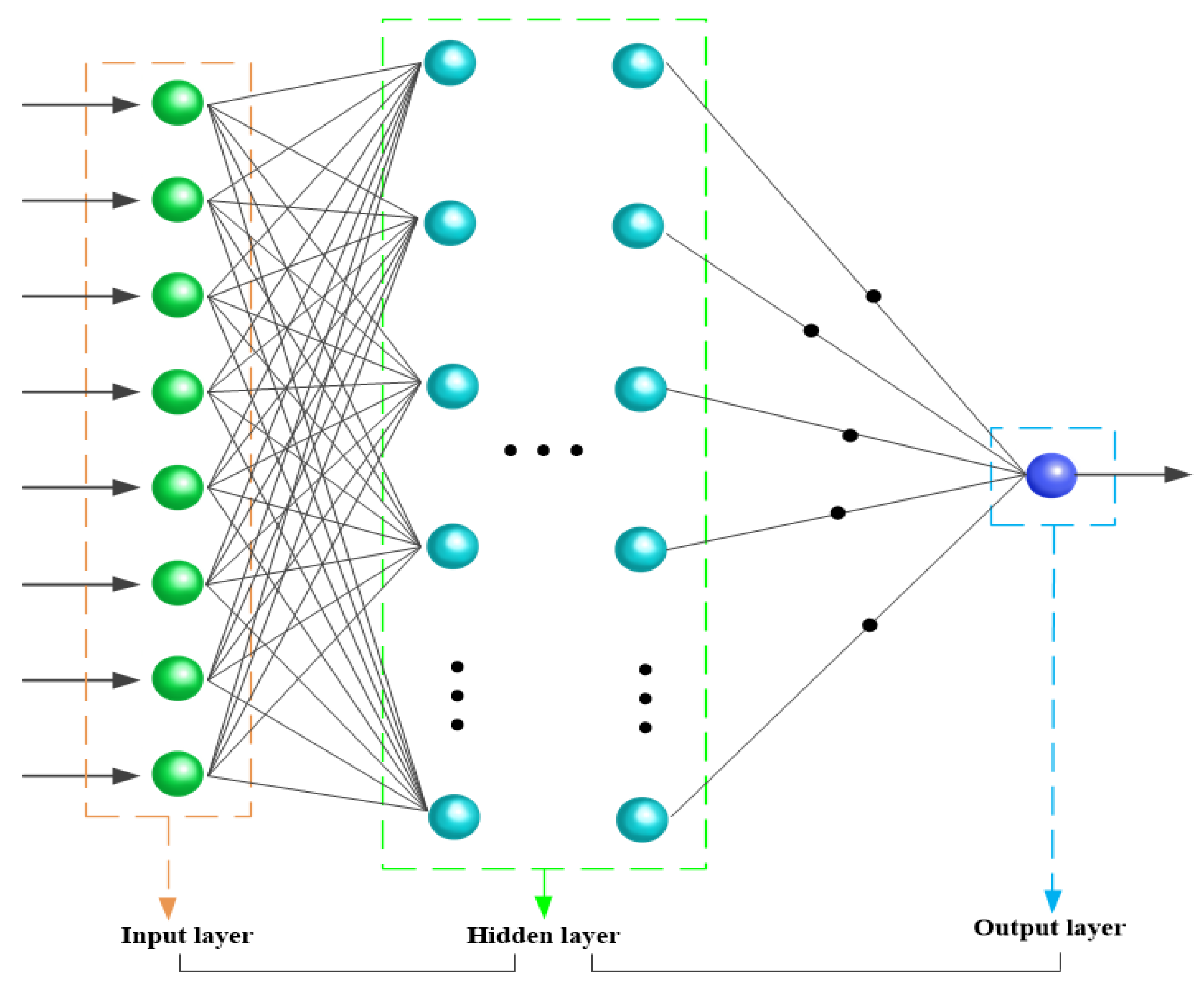
BP neural network is the foremost representative artificial neural network with three or more layers, including the input layer, the hidden layer, and the output layer. Neurons connect fully on the same layer and are not connected between the different layers. The signal starts from the input layer nodes and transmits to the output layer nodes after passing the hidden layer nodes [32]. BP neural network, with its self-organizing ability, can automatically find patterns in the input information without any a priori knowledge, adjust the connection weights between the processing units according to the back propagation of errors, and after a period of self-learning training or perception, form a nonlinear model suitable for expressing the patterns and produce reasonable output values based on the given input information. In the process of processing information, it is adaptive and fault-tolerant, allowing a certain amount of inaccurate or even wrong information, and it can approximate any function, which makes comprehensive, dynamic, and fuzzy evaluations with large amounts of data have a scientific basis. Compared with traditional scoring and evaluation methods, BP neural network overcomes the deficiency of subjectivity in the initial evaluation process. It only requires a small number of training samples to determine the weights and thresholds with a high degree of accuracy, and could achieve any complex nonlinear function fitting with any accuracy, truthfully reflecting and approaching the reality, with scientific, objective, and reliable characteristics [33,34,35]. A typical structure of three layers in the BP neural network model is shown in Figure 1.

This paper uses a three-layer BP network to realize an arbitrary function approximation to evaluate the agricultural investment climate of CEE countries. The number of input layer nodes is set for n. The number of hidden layer nodes is set for m. The number of output layer nodes is set for p.

Kolmogorov theorem proves that for a given arbitrary continuous function ϕ: $E^n\to R^m$, ϕ(x) = y, ϕ could be precisely realized by a three-layer neural network. In other words, a neural network with only one nonlinear hidden layer can approximate a function of arbitrary complexity with arbitrary accuracy [36,37]. The selection of hidden nodes is a challenging issue. If the number of hidden nodes is relatively small, it may lead to poor training effect of the BP neural network. If the number of hidden nodes is large, although it could reduce the training error of the system, the training efficiency of the BP neural network would be reduced, since the network training will be stuck in the local minima and will not be optimized, which will eventually lead to the phenomenon of overfitting. The basic principle for determining the number of hidden layer nodes is to achieve a structure as compact as possible while meeting the accuracy requirements, i.e., to have as few hidden layer nodes as possible. The number of hidden nodes could be obtained from the empirical formula of Kolmogorov theorem:

$$m=\sqrt{n+p+1}+c$$

(1)

In this formula, c is within the scope of 1–10 constant. BP network learning process comprises of signal forward-propagation process and error back-propagation process. The error signal ceaselessly decreases the following iterations and consequently the network training ends when the error is less than the acceptable value.

The hidden layer and output layer obtained the Tan-Sigmoid formula and the linear formula as transfer function respectively. The neuron’s outputs can be expressed as:

$$\text{Hidden Layer }{x}_i=\sigma ({\displaystyle \sum }_{j=1}^n{w}_{ij}^0{x}_j+w_{i0}^0) i = 1, 2, \dots , m; j = 1, 2, \dots , n$$

(2)

In this formula, x_i is the output i of neurons; x_j is the input j of neurons; $w_{ij}^{0 }$ are connection weights of the j nodes of the input layer to the i nodes of the hidden layer; and $w_{i0 }^0$ is the threshold value of the i node of neurons. σ denotes the Tan-Sigmoid function.

$$\text{Output Layer }{y}_h={\displaystyle \sum }_{k=1}^m{w}_{hk}^0{x}_k+w_{h0}^0 h = 1, 2, \dots , p; k = 1, 2, \dots , m$$

(3)

In this formula, y_h is the output h of neurons; x_k is the input k of neurons; $w_{hk}^0$ are connection weights of the k nodes of the input layer to the h nodes of the output layer; and $w_{h0}^0$ is the threshold value of the h node of neurons.

2.1.2. BP Neural Network Algorithm

To realize the minimum mean square error between each sample’s target and final output, the BP neural network’s connection weights are required to adjust. When applying BP neural network evaluation, the self-learning process is finally completed by literately modifying the network parameter settings. Each layer’s connection weights are adjusted until the minimum mean square error of the final network output reaches an acceptable level. The learning rule of BP neural network requires adjusting weights along the function’s negative gradient direction, which will diminish the function value fastest to explore suitable weights and acquire results more quickly.

Assume p is the number of training samples, and the input and output mode of the kth group of samples are used to train the network. The convergence error bound value is set for ε_min, and maximum number of learning for N. According to the error function, the sample error after iterative computation can be represented by $E_k=\frac{1}{2}{\displaystyle \sum }_{i=1}^n\left(h_{oi}\left(k\right)-y_{oi}\left(k\right)\right)$ and training error $E= \frac{1}{P}{\displaystyle \sum }_{K=1}^P{E}_K$ could be obtained. If the error between the network output value and the desired output value does not accomplish the error accuracy prerequisite, it will shift to error reverse propagation. Meanwhile, connection weights and threshold values are continuously amended by the end that the error meets accuracy necessity. Connection weights and threshold correction formula are as follows:

$${\Delta }_w\left(t+1\right)=\eta {\delta }_{jk}{o}_{ik}+\alpha {\Delta }_k{w}_{ij}\left(t\right)$$

(4)

$${\theta }_j\left(t+1\right)={\theta }_j+\frac{1}{p}{\displaystyle \sum }_{k=1}^p{\Delta }_k{\theta }_j$$

In this formula, η is the learning rate and α is the momentum factor, which are somewhere in the range 0 and 1; $\alpha {\Delta }_k{w}_{ij}\left(t\right)$ is momentum term; ${\delta }_{jk}$ is output node calculation error; and t is training times.

Initializing the input values will be taken note of in developing the BP neural network. BP network is one of the most generally utilized neural networks for the present, and it is delicate in selecting parameters. Therefore, choosing appropriate training values becomes especially significant.

2.2. Entropy Method

The entropy weighting method is an objective weighting method, the basic idea of which is to determine the objective weight according to the variability of the indicator. It is based on the principle that the smaller the variability of an indicator, the less information it reflects, and the lower the corresponding weight should be. The process to generate comprehensive agricultural investment climate evaluation grade according to entropy method included the following steps.

• Step 1: Data selection

Set the number of indicators as m and number of samples as n. X_ij is the value of jth indicator of the ith sample, i = 1, 2, 3, …, n; j = 1, 2, 3, …, m.

• Step 2: Data standardization processing

In cases where the units of measurement and direction of the indicators are not uniform, the data need to be standardized, and to avoid meaningless logarithms for the entropy values, a smaller order of magnitude of real numbers can be added to each 0.00 value, e.g., 0.01 or 0.0001.

For positive indicators (a higher value indicates a better performance):

$${\mathrm{X}}^{\prime }= \frac{X_{ij}-Min\left(X_{ij}\right)}{Max\left(X_{ij}\right)-Min\left(X_{ij}\right)}$$

(5)

For negative indicators (a lower value indicates a better performance):

$${\mathrm{X}}^{\prime }= \frac{Max(X_{ij})-X_{ij}}{Max\left(X_{ij}\right)-Min\left(X_{ij}\right)}$$

(6)

• Step 3: Weight calculation of each sample

Calculate the weight of the ith sample under indicator j:

$$P_{ij}=\frac{X_{ij}}{{{\displaystyle \sum }}_{i=1}^n{X}_{ij}}$$

(7)

• Step 4: Entropy value calculation of the indicators

Calculation of the entropy value of indicator j:

$$e_j=-k{{\displaystyle \sum }}_{i=1}^n\left(p_{ij}*\ln \left(p_{ij}\right)\right)$$

(8)

In this formula, K = $\frac{1}{\ln \left(n\right)}$, and n is the number of samples.

• Step 5: Calculation of the variance factor for indicator j

The information utility value of an indicator depends on the difference between the information entropy $e_j$ and 1 for that indicator, and its value directly affects the weighting. The greater the information utility value, the greater the importance to the evaluation and the greater the weighting.

$$d_j=1-e_j$$

(9)

• Step 6: Weight calculation of each indicator

The essence of estimating indicator weights using the entropy method is to use the coefficient of variation of the information for that indicator; the higher the coefficient of variation, the more important it is for evaluation.

$$w_j=\frac{d_j}{{{\displaystyle \sum }}_{j=1}^m{d}_j}$$

(10)

• Step 7: Composite score calculation for each sample

$$z_i={{\displaystyle \sum }}_{j=1}^m{w}_j{x}_{ij}$$

(11)

2.3. The Agricultural Investment Climate Evaluation Model Based on BP Neural Network

Through analyzing, surveying and reviewing pertinent literature on the premise of defining agricultural investment climate, completing the correlation analysis of the indicator data and verifying the rationality of the testing indicator system, we build a three-level evaluation index system for the agricultural investment climate in CEE countries. The system divides the agricultural investment climate into four subsystems: the political, economic, social, and technical climates. The agricultural investment climate evaluation index system with a total of 22 indicators is shown in

Table 1. Agricultural investment climate evaluation index system.

Primary Indicator	Secondary Indicator	Tertiary Level Indicator
Political Climate A1	Political stability B1	Political Stability C1
		Government Effectiveness C2
	Governmental service B2	Burden of government regulation C3
		Regulatory Quality C4
		Control of Corruption C5
Economic Climate A2	Market size and openness B3	GDP per ca pita (current US$) C6
		Extent of market dominance C7
		Prevalence of non-tariff barriers C8
	Business climate B4	Cost of starting a business C9
		Procedures of starting a business C10
		Strength of minority investor protection C11
		Venture capital availability C12
Social Climate A3	Legal institution B5	Rule of Law C13
		Efficiency of legal framework in settling disputes C14
		Efficiency of legal framework in challenging regulations C15
	Employment Relationship Dynamics B6	Hiring and firing practices C16
		Cooperation in labor-employer relations C17
Technical Climate A4	Infrastructure level B7	Quality of road infrastructure C18
		Efficiency of train services C19
		Electricity supply quality C20
	Information level B8	Internet users (% of adult population) C21
		Information development index C22

.

According to the agriculture invest climate evaluation index system, corresponding BP neural network is a representative three-layer feed-forward network, where the number of input nodes can be depicted by m = 22 and the output layer has a comprehensive evaluation value, namely the number of nodes described by n = 1, while the number of hidden nodes is resolved to be e = 15 by Formula (1) and the length of training convergence time. The results of network training and testing for the hidden layer nodes are shown in

Table 2. Verification of the number of nodes in the hidden layer of BP neural network.

Average Results (Ten Times)	Number of Hidden Layer Nodes
	8	9	10	11	12	13	14	15	16
Training times	29.6	29.3	19.3	19.7	13.8	13.5	12.5	8.6	13.9
Mean square error	0.0553	0.0193	0.0627	0.0468	0.0247	0.0815	0.0352	0.0111	0.0363

. Hence, the BP neural network model structure that assesses the agriculture invest climate should be 22 × 15 × 1.

2.4. Selection of Evaluation Objects and Data Sources

Based on the current geographical distribution of CEE countries, 16 countries were selected for evaluation after considering the potential placement of China’s outward investment in agriculture in terms of reality, resources and policies. The 2009–2018 basic data are mainly from authoritative data published by the World Bank, the World Economic Forum and International Telecommunication Union. Among them, C1, C2 and C5 are drawn from the World Bank’s World Governance Indicators; C6 from the World Bank database; C16 and C17 from the World Bank’s Doing Business report; C22 from the International Telecommunication Union’s Measuring the Information Society report; and the rest from the World Economic Forum’s Global Competitiveness Index indicators.

2.5. Model Simulation

2.5.1. Determination of Classical Domain

With reference to the evaluation criteria of the corresponding indicators in the authoritative database and the statistical results of the indicator data of the CEE countries in the period 2009–2018, then 16 samples are obtained. The classical domain refers to the value range of the indicators. The classical domain matter-element matrix R_N is shown as follows:

$${\mathrm{R}}_{\mathrm{N}}=\left\{\begin{array}{ccc}{N}_i& C_1& \left(a_{i1},b_{i1}\right)\\ & C_2& \left(a_{i2},b_{i2}\right)\\ & \begin{array}{c}\dots \\ C_n\end{array}& \begin{array}{c}\dots \\ \left(a_{in},b_{in}\right)\end{array}\end{array}\right\}$$

(12)

where $N_i$ represents the divided evaluation Level I; $C_1$, $C_2$, …, $C_n$ represent the evaluation indexes; and ($a_{in},b_{in}$) represents the value range of the evaluation index for the evaluation Level i, namely the classical domain. The state of agricultural investment climate indicators is divided into four levels. The value of these level is presented in

Table 3. The classical domain of agricultural investment climate evaluation index.

Level	C1	C2	C3	C4	C5
I	[0.63, 1.12]	[0.71, 1.19]	[1.22, 1.70]	[4.12, 4.88]	[0.95, 1.51]
II	[0.15, 0.63)	[0.22, 0.71)	[0.76, 1.22)	[3.37, 4.12)	[0.39, 0.95)
III	[−0.33, 0.15)	[−0.26, 0.22)	[0.27, 0.76)	[2.61, 3.37)	[−0.17, 0.39)
IV	[−0.82, −0.33)	[−0.74, −0.25)	[−0.21, 0.27)	[1.85, 2.61)	[−0.73, −0.17)
Level	C6		C7	C8	C9	C10
I	[20529.11, 26054.54]		[4.41, 5.06]	[5.35, 5.91]	[75, 100]	[0.39, 0.5]
II	[15003.67, 20529.11)		[3.77, 4.41)	[4.79, 5.35)	[50, 75)	[0.28, 0.39)
III	[9478.24, 15003.67)		[3.12, 3.77)	[4.23, 4.79)	[25, 50)	[0.17, 0.28)
IV	[3952.80, 9478.24)		[2.47, 3.12)	[3.67, 4.23)	[0, 25)	[0.06, 0.17)
Level	C11	C12	C13	C14	C15	C16
I	[34, 41]	[3.33, 3.83]	[0.90, 1.37]	[3.29, 4.38]	[3.41, 4.52]	[4.68, 5.48]
II	[27, 34)	[2.83, 3.33)	[0.43, 0.90)	[2.21, 3.29)	[2.30, 3.41)	[3.88, 4.68)
III	[20, 27)	[2.33, 2.83)	[−0.05, 0.43)	[1.12, 2.21)	[1.19, 2.30)	[3.08, 3.88)
IV	[13, 20)	[1.83, 2.33)	[−0.52, −0.05)	[0.03, 1.12)	[0.07, 1.19)	[2.28, 3.08)
Level	C17	C18	C19	C20	C21	C22
I	[4.66, 5.16]	[4.64, 5.62]	[3.83, 4.74]	[5.33, 6.51]	[69.5, 88.4]	[7.02, 8.16]
II	[4.16, 4.66)	[3.66, 4.64)	[2.92, 3.83)	[4.16, 5.33)	[50.7, 69.5)	[5.88, 7.02)
III	[3.66, 4.16)	[2.68, 3.66)	[2.01, 2.92)	[2.98, 4.16)	[31.9, 50.7)	[4.75, 5.88)
IV	[3.16, 3.66)	[1.70, 2.68)	[1.10, 2.01)	[1.80, 2.98)	[13.1, 31.9)	[3.61, 4.75)

.

2.5.2. The Training Phases

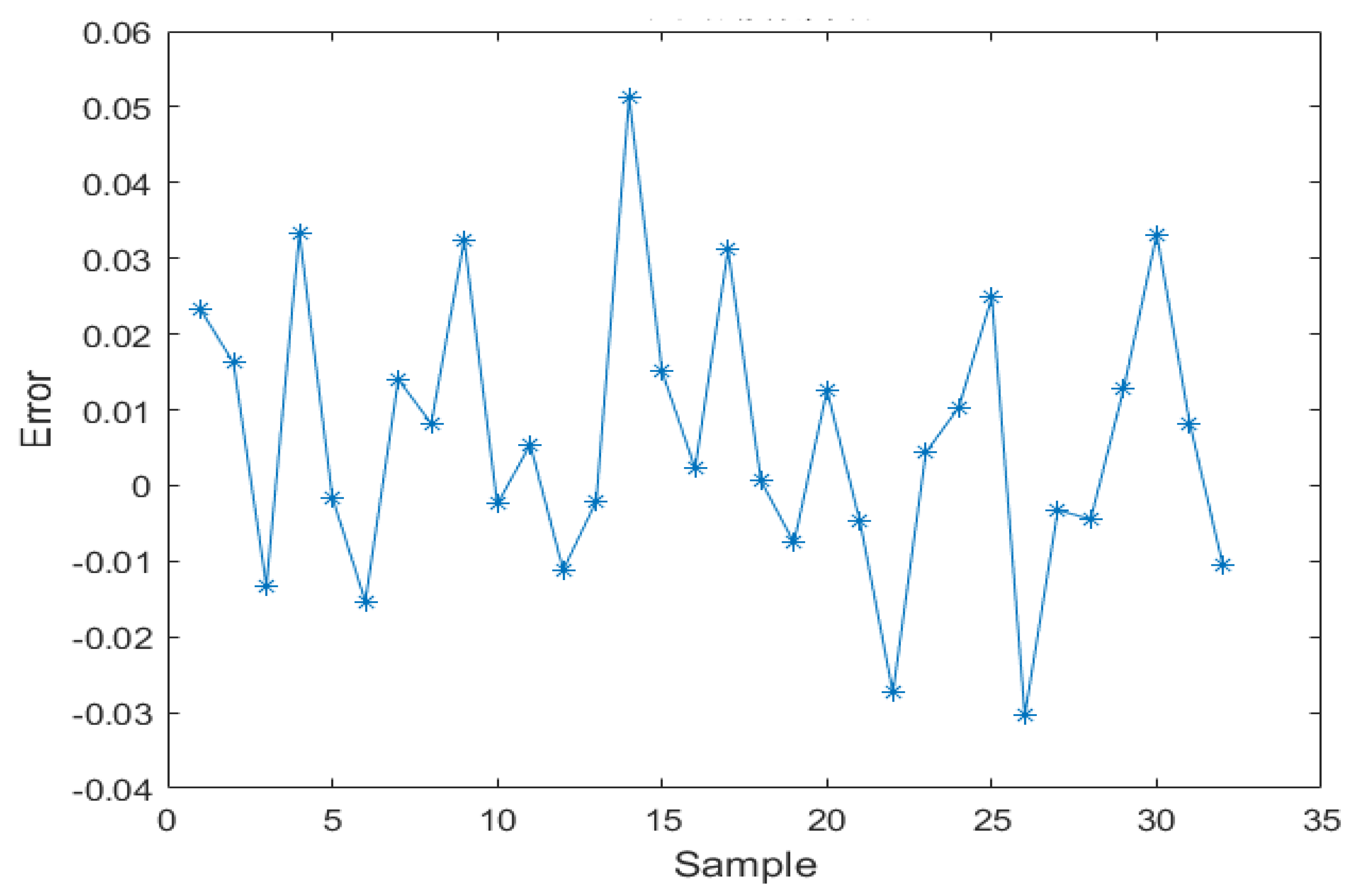
The BP network is built according to the above settings, and the raw data is standardized using the polar method. The 22 variables and indicators of the four subsystems of the evaluation index system were used as input vectors, and the comprehensive agricultural investment climate evaluation grade generated according to entropy method was used as output vectors. The network structure of 22 × 15 × 1 is selected in the BP neural network training phase. Set the maximum number of training for N = 1000, learning rate for η = 0.01, momentum factor for α = 0.5, and minimum convergence error for ε_min = 10⁻⁴. Transfer function is the logsig function of the logarithm of S; training function is the traingdx function, learning function is the learndm function, and the initial value of weight matrix is given by the system. The simulation results of the BP network model are obtained from Matlab. The 10-year data of the 16 countries total 160 groups, among them 128 groups are selected as train samples, and the rest as test samples. The predicted output and error of BP neural network is shown in Figure 2 and Figure 3.

2.5.3. The Test Phases

There are a lot of performance measure methods that could be utilized to evaluate the accuracy. Therefore, we choose two metrics in this study: the mean square error (MSE) and mean absolute percentage error (MAPE) to comprehensively test the network performance. MSE is a measure of the average of the prediction error squares; it can assess the variation of the model. A smaller MSE value represents a better prediction of the model. MAPE is a measure of the accuracy of the prediction methods used in statistics for performance evaluation and comparison.

$$MSE=\frac{1}{N}{\displaystyle \sum _{n=1}^N}{\left(y_n-{\widehat{y}}_n\right)}^2$$

(13)

$$MAPE=\frac{1}{N}{\displaystyle \sum }_{n=1}^N\left|\frac{y_n-{\widehat{y}}_n}{y_n}\right|\times 100\%$$

(14)

where $y_n$ and ${\widehat{y}}_n$ represent output value and predicted value of nth data for agricultural investment climate evaluation. N is the total number of data used for agricultural investment climate evaluation. The results are listed in

Table 4. BP neural network performance evaluation results (10 random times).

Sample	Mean Square Error	Mean Absolute Percentage Error (%)
Training sample	0.0041	0.4012
Test sample	0.0062	0.4513

.

Through network training, the threshold values of the agricultural investment climate evaluation index in Table 3 were simulated and calculated, and the output results were used as the basis to classify the levels of CEE countries’ agricultural investment climate. According to the critical value of agricultural investment climate level simulation results, the evaluation level is divided into I–IV degree. The threshold results are shown as follow:

-

Level I. good investment climate (≥ 0.6484)

-

Level II. relatively good investment climate (0.4885, 0.6484)

-

Level III. relatively poor investment climate (0.3285, 0.4885)

-

Level IV. poor investment climate (≤ 0.3285)

A good investment climate reflects that the overall climate is suitable for agricultural investment, and a relatively good investment climate reflects that only a few issues in the investment climate require attention. A relatively poor investment climate represents the regional investment climate that needs investors’ careful consideration, while a poor investment climate refers to the overall climate for investment that needs to be improved.

3. Results and Discussion

With the above-trained BP neural network model, the data of each indicator of the average level of the 16 evaluation objects during 2009–2018 were used as test samples and substituted into the trained network to obtain the corresponding output values, which were compared with the critical values to obtain the comprehensive evaluation results and the agricultural investment climate rating of each subsystem.

3.1. Synthesis of Evaluation Findings and Analysis

In order to fully take into account the variation of influencing factors in different years, this paper introduces the data from 2009 to 2018 into the model based on dynamic thinking, which not only meets the systematic requirement of investment climate evaluation, but also effectively reduces the inconsistency of longitudinal comparison brought about by the assignment of cross-sectional data, and realizes the improvement of the accuracy of investment climate evaluation. According to the results in

Table 5. Evaluation results of investment climate of CEE countries 2009–2018.

	2009	2010	2011	2012	2013	2014	2015
Albania	0.2955	0.3397	0.3664	0.3530	0.3072	0.2824	0.3638
Bosnia and herzegovina	0.1691	0.1784	0.1593	0.2284	0.2733	0.2177	0.1451
Bulgaria	0.3480	0.3314	0.3212	0.3402	0.3357	0.3020	0.3051
Croatia	0.4630	0.4484	0.4420	0.4400	0.4627	0.4429	0.3992
Czech	0.6553	0.6635	0.6438	0.6295	0.6153	0.6296	0.6581
Estonia	0.7518	0.7908	0.8027	0.7930	0.7998	0.8097	0.8056
Hungary	0.5454	0.5699	0.5724	0.5347	0.5263	0.5282	0.5133
Latvia	0.5873	0.5772	0.6005	0.6372	0.6423	0.6377	0.6266
Lithuania	0.5796	0.5771	0.5561	0.6148	0.6026	0.5805	0.6078
Montenegro	0.4073	0.4695	0.4662	0.4647	0.4334	0.4019	0.3855
Macedonia	0.3812	0.4113	0.3949	0.4002	0.4109	0.4622	0.4185
Poland	0.5114	0.5360	0.5217	0.5397	0.5571	0.5537	0.5516
Romania	0.4121	0.3672	0.3265	0.2883	0.3169	0.3595	0.3783
Serbia	0.2563	0.2440	0.2273	0.2224	0.2332	0.2430	0.2182
Slovakia	0.6406	0.6086	0.5690	0.5744	0.5377	0.5262	0.5042
Slovenia	0.8299	0.7569	0.6950	0.6946	0.6718	0.6573	0.6700
	2016	2017	2018	Average	Rank	Relative Change (2009/2018)/Rank
Albania	0.3859	0.3966	0.4183	0.3509	13	41.6%	1
Bosnia	0.1101	0.1178	0.0982	0.1697	16	−41.9%	16
Bulgaria	0.3486	0.3403	0.3396	0.3312	14	−2.4%	10
Croatia	0.3900	0.3694	0.3667	0.4224	10	−20.8%	13
Czech	0.6536	0.6452	0.6513	0.6445	3	−0.6%	8
Estonia	0.8324	0.8433	0.8546	0.8084	1	13.7%	3
Hungary	0.4656	0.4869	0.4726	0.5215	8	−13.3%	11
Latvia	0.6045	0.5659	0.6191	0.6098	4	5.4%	6
Lithuania	0.6183	0.5751	0.6023	0.5914	5	3.9%	7
Montenegro	0.3794	0.3863	0.4461	0.4240	9	9.5%	4
Macedonia	0.3986	0.3308	0.2647	0.3873	11	−30.6%	15
Poland	0.5550	0.5518	0.5427	0.5421	7	6.1%	5
Romania	0.3456	0.3416	0.4026	0.3539	12	−2.3%	9
Serbia	0.2294	0.2732	0.3154	0.2463	15	23.0%	2
Slovakia	0.5018	0.4908	0.5036	0.5457	6	−21.4%	14
Slovenia	0.6926	0.6941	0.7102	0.7072	2	−14.4%	12

, among the CEE countries, two countries scored at Level I overall, including Estonia and Slovenia. Six countries in Level II, including the Czech Republic, Hungary, Latvia, Lithuania, Poland, and Slovakia, and six countries in Level III, including Albania, Bulgaria, Croatia, Montenegro, North Macedonia and Romania. Two countries were evaluated at level IV, including Bosnia and Herzegovina and Serbia.

Table 5 shows the ranking of CEE countries in terms of agricultural investment climate scores, average values and relative change from 2009 to 2018. The agricultural investment climate in CEE countries is generally high in the three Baltic countries, significantly higher than in the Visegrad Group and Slovenia, as well as in the Balkans. Among the 16 countries, Estonia has a stable rating and is the long-term leader. Slovenia and the Czech Republic follow closely behind. In terms of the overall improvement of the investment climate, Albania’s agricultural investment climate score was only 0.2954 in 2009, but after 10 years of optimization, its overall index has increased by 41.6%, showing great enthusiasm for improving the investment climate. After Albania, the agricultural investment climate in Serbia and Estonia also shows positive trends. Although the Balkans lags behind among the 16 countries in terms of its investment climate score, the increase in the score over the past 10 years reflects a particular potential for optimization, and there is still room for further improvement in the future.

On the one hand, the performance is closely related to stable political climate, free and open economic climate, large market size, relatively sound investment regulations, and generally better infrastructure conditions in different countries. On the other hand, it is also benefited by the export structure of international agricultural capital. This finding also reflects the differences in economic development, openness to the outside world, infrastructure construction, public services, and agricultural resources of the 16 target countries evaluated, which are the main aspects that determine the agricultural investment climate.

3.2. Subsystem Evaluation Findings and Analysis

The agricultural climate evaluation based on BP neural network could make a more objective understanding of the political, economic, social, and technical climate of the current development in CEE countries.

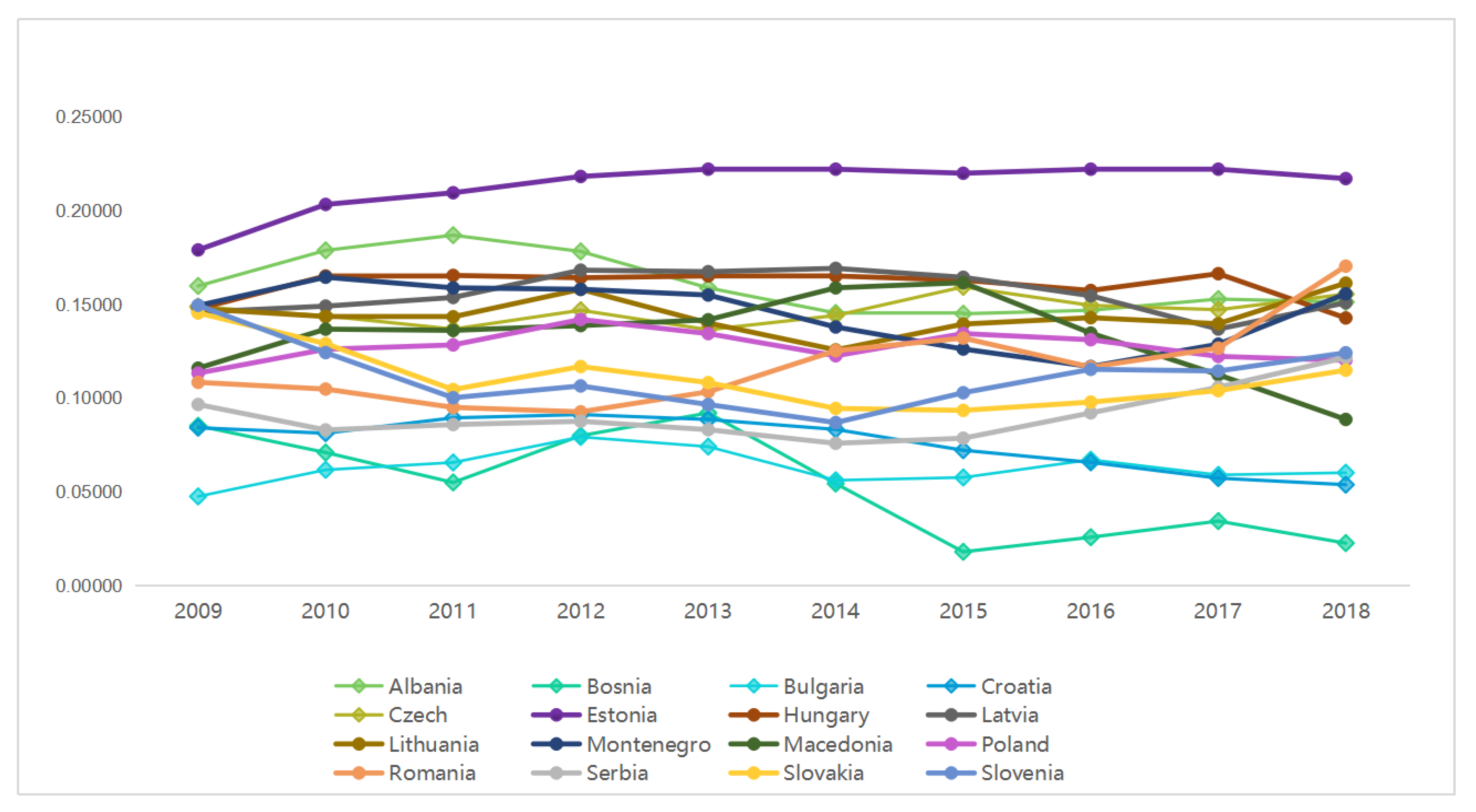
3.2.1. Findings and Analysis of the Political Climate Evaluation

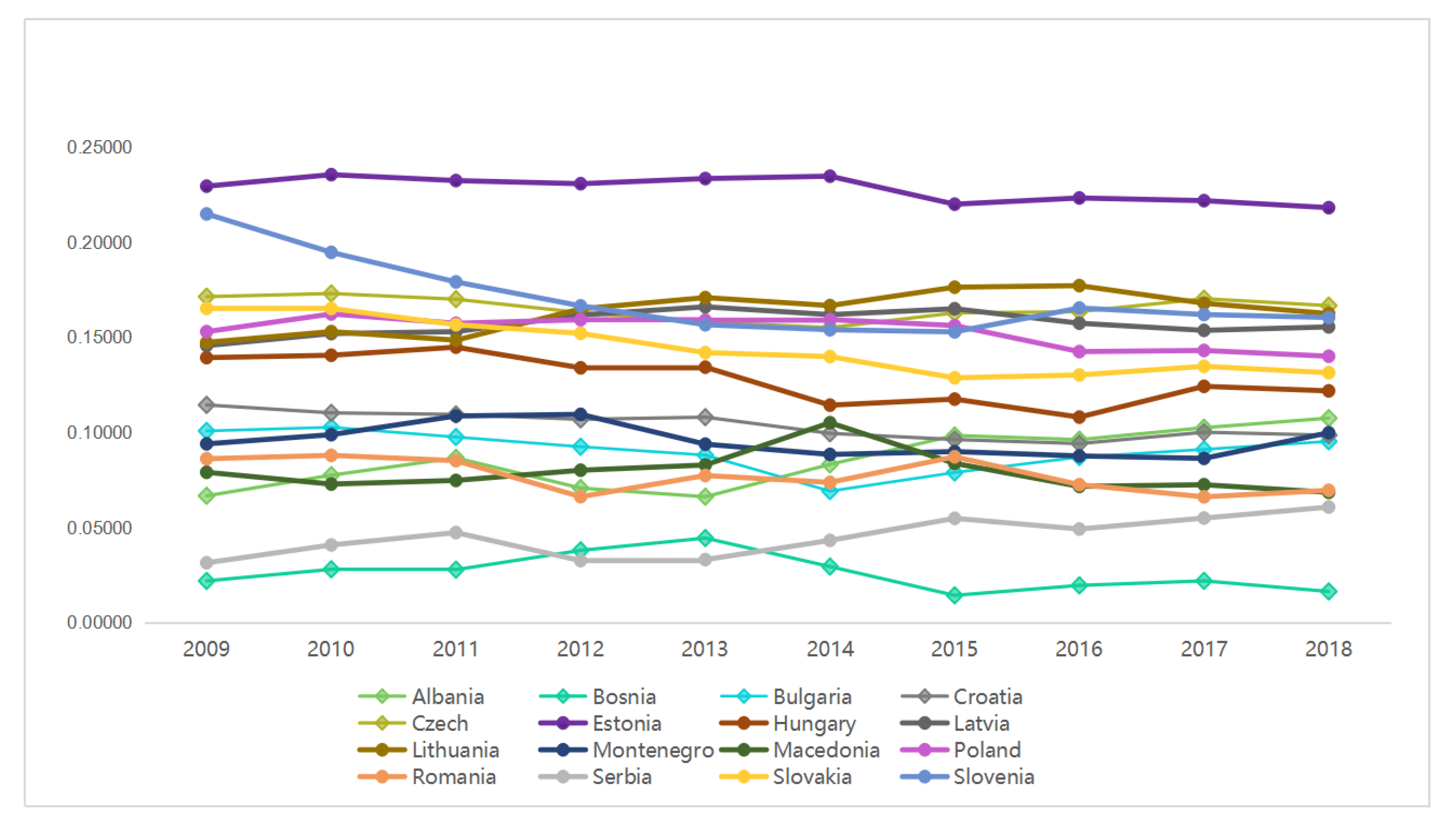
The political climate evaluation result is shown in Figure 4 and

Table 6. Average evaluation results of political climate in CEE countries.

Country	Ave.	Rank	Relative Change (2009/2018)	Country	Ave.	Rank	Relative Change (2009/2018)
Albania	0.0855	12	61.2%	Lithuania	0.1634	4	10.3%
Bosnia	0.0262	16	−25.2%	Montenegro	0.0957	10	6.2%
Bulgaria	0.0902	11	−5.4%	Macedonia	0.0791	13	−13.3%
Croatia	0.1037	9	−13.9%	Poland	0.1531	6	−8.4%
Czech	0.1652	3	−2.7%	Romania	0.0772	14	−19.3%
Estonia	0.2278	1	−4.9%	Serbia	0.0449	15	93.0%
Hungary	0.1278	8	−12.5%	Slovakia	0.1445	7	−20.5%
Latvia	0.1570	5	6.8%	Slovenia	0.1705	2	−25.3%

. The Baltic countries remain ahead of the rest of the countries. Estonia performs the best in this indicator, with an average score of 0.2278 from 2009 to 2018, significantly higher than other countries’ level. Lithuania and Latvia are ranked fourth and fifth in CEE countries with scores of 0.1634 and 0.1571, respectively, showing a relatively complete institutional supply capacity. Slovenia, the Czech Republic, and Poland ranked second, third, and sixth out of 16 countries with scores of 0.1705, 0.1652, and 0.1531, which indicate an ideal institutional climate. The institutional supply capacity of Balkan countries is relatively low among the 16 countries. All of the countries in the Balkans are in the low level, among which Bosnia and Herzegovina has the lowest score, with a 10-year average score of only 0.0262. Their level of political resource supply needs to be optimized. At the same time, in terms of dynamics, the Balkans are the most optimized region as a whole. Serbia, Albania and Montenegro rank first, second and fifth among CEE countries with 93.0%, 61.2% and 6.2% growth rates, respectively. The Visegrad Group and Slovenia have experienced a deterioration in institutional supply. The sharpest decline was in Slovenia, which, with a negative growth rate of 25.3%, was the most severe decline in political resource availability among the 16 CEE countries.

3.2.2. Findings and Analysis of the Economic Climate Assessment

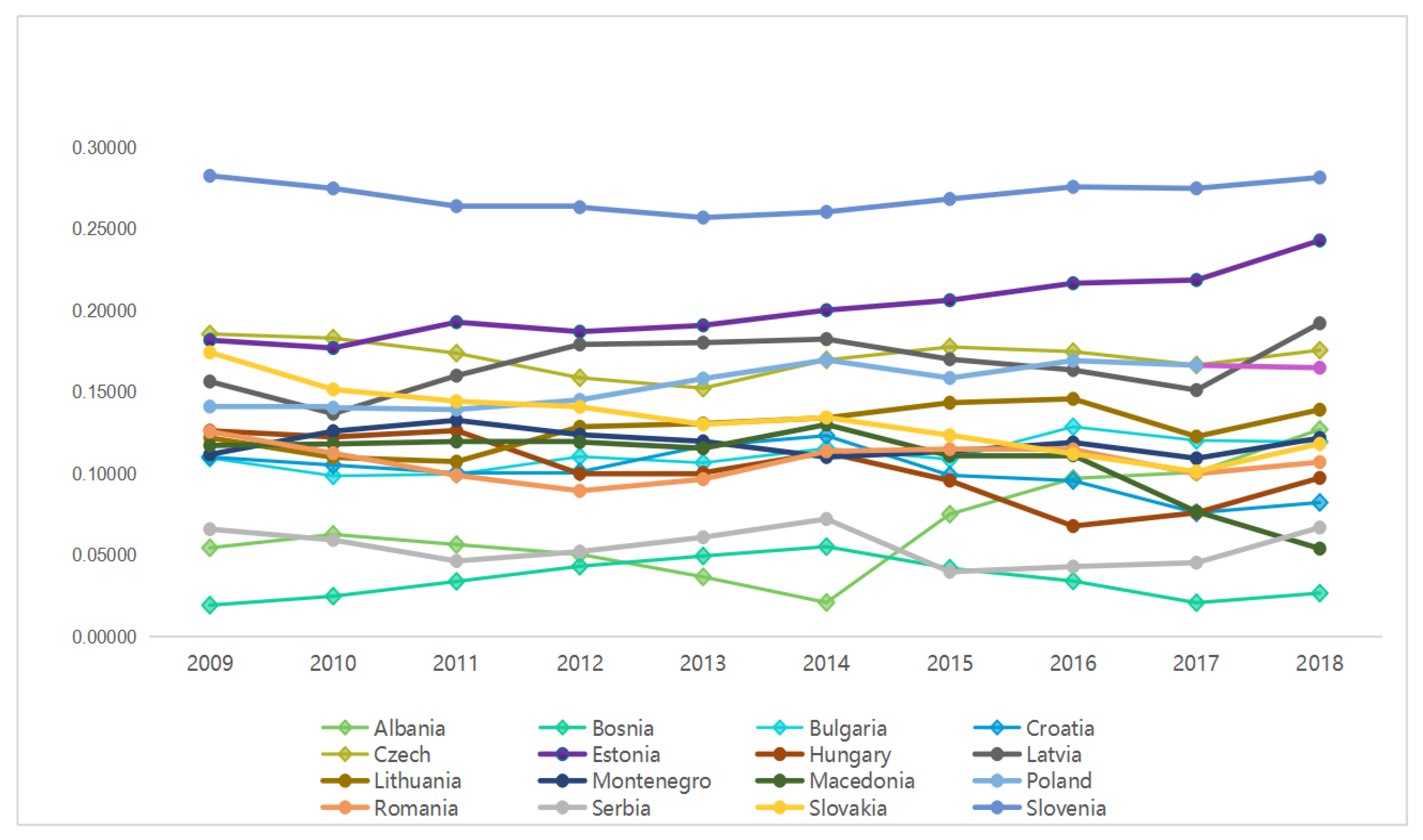
The economic climate evaluation result is shown in Figure 5 and

Table 7. Average Evaluation results of economic climate in CEE countries.

Country	Ave.	Rank	Relative Change (2009/2018)	Country	Ave.	Rank	Relative Change (2009/2018)
Albania	0.0681	14	133.6%	Lithuania	0.1283	7	14.2%
Bosnia	0.0348	16	38.7%	Montenegro	0.1187	8	9.0%
Bulgaria	0.1117	9	9.0%	Macedonia	0.1072	11	−54.0%
Croatia	0.1009	13	−25.3%	Poland	0.1552	5	16.9%
Czech	0.1717	3	−5.4%	Romania	0.1073	10	−14.9%
Estonia	0.2014	2	33.7%	Serbia	0.0551	15	1.5%
Hungary	0.1024	12	−22.9%	Slovakia	0.1330	6	−32.2%
Latvia	0.1672	4	22.8%	Slovenia	0.2703	1	−0.4%

. The Baltic countries are on par with the Visegrad Group and Slovenia on the whole. However, in 2018, the mean value of the five countries’ economic resources and climate in the Visegrad Group and Slovenian segment was 0.1674, slightly lower than the Baltic Three mean value of 0.1913. In terms of country performance, in 2018, Slovenia had a score of 0.2815. The Czech Republic and Poland topped the list of CEE countries with a score of 0.1755 and 0.1648, respectively, and were ranked fourth and fifth among the 16 countries. The Czech Republic takes the top spot in CEE in terms of the 10-year average score. The three Baltic countries also performed well. They had the highest average regional scores in 2018, and all three countries were ranked among the top six countries in CEE countries. In 2018, the Balkan countries’ average score was only 0.0881, ranking last in the three sectors. Even in the highest-scoring Albania, the economic resources and climate index was only 0.1269, ranked seventh in CEE countries. Bosnia and Herzegovina had a single-year score of 0.0265 and a 10-year average score of 0.0348 at the bottom of 16 countries, with certain problems in the domestic investment and business climate. Although most countries have improved their scores in this indicator in recent years, there are still six countries with declines in their scores. Macedonia has become the most obvious country with a 38.4% drop in this indicator, which indicates its economic climate has to be strengthened.

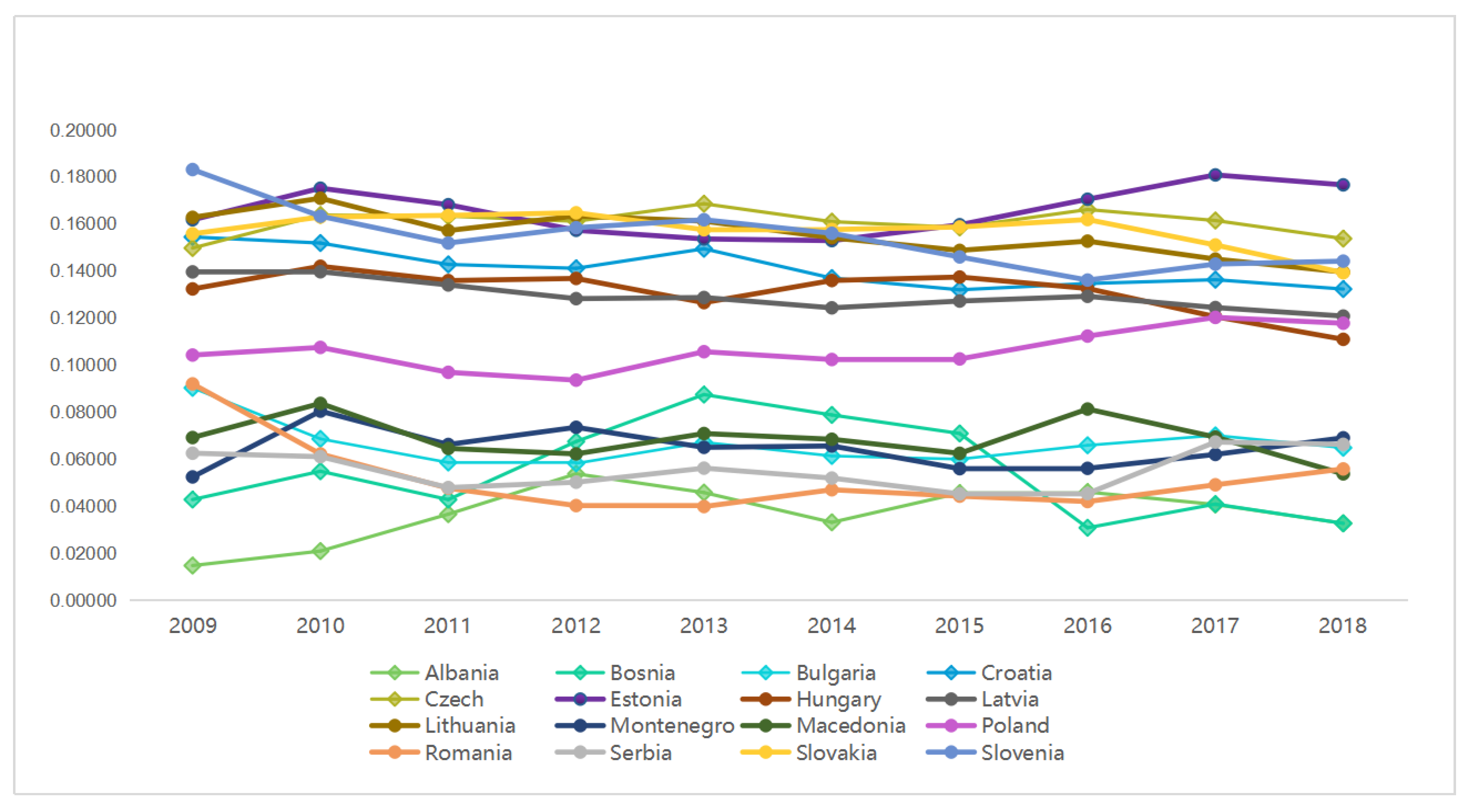
3.2.3. Findings and Analysis of the Social Climate Assessment

The social climate evaluation result is shown in Figure 6 and

Table 8. Average evaluation results of social climate in CEE countries.

Country	Ave.	Rank	Relative Change (2009/2018)	Country	Ave.	Rank	Relative Change (2009/2018)
Albania	0.1604	2	−5.4%	Lithuania	0.1441	7	9.2%
Bosnia	0.0538	16	−73.5%	Montenegro	0.1451	6	4.2%
Bulgaria	0.0628	15	26.6%	Macedonia	0.1325	8	−2.7%
Croatia	0.0767	14	−36.1%	Poland	0.1274	9	6.0%
Czech	0.1468	5	4.5%	Romania	0.1175	10	57.2%
Estonia	0.2135	1	21.3%	Serbia	0.0910	13	25.9%
Hungary	0.1602	3	−3.3%	Slovakia	0.1109	12	−21.0%
Latvia	0.1560	4	3.4%	Slovenia	0.1121	11	−16.9%

. The Baltic countries continue to perform the best overall with an average score of 0.1764 in 2018, which is higher than 0.1314 of the Visegrad Group and Slovenian segment, and 0.0919 of the Balkans. Estonia scores 0.2170 in 2018, which has achieved the leading position in this indicator for 3 years. With scores in third and seventh place in 16 countries, Lithuania and Latvia have a stable overall performance and are in the middle to upper range of CEE countries. Within the Visegrad Group and Slovenia segment, the Czech social resource market is the most prominent performer, with a score of 0.1554 that places it in the fifth position of CEE countries in 2018. Although most Balkan countries have relatively low scores in this indicator, Albania has a favorable labor market climate, with a score of 0.1512 in 2018, ranking it sixth in 16 countries and a mean score of 0.1604 between 2009 and 2018, moving it to the second place among the 16 countries. Meanwhile, the Balkan countries outperform other regions in terms of indicator improvement, with Romania, Bulgaria, Serbia, and Montenegro achieving social resource market optimization. Thus, the improvements positively influence the further reduction of the differences in the labor market climate in CEE countries and promote regional coordination.

3.2.4. Findings and Analysis of Technical Climate Assessment

The technical climate evaluation result is shown in Figure 7 and

Table 9. Average evaluation results of technical climate in CEE countries.

Country	Ave.	Rank	Relative Change (2009/2018)	Country	Ave.	Rank	Relative Change (2009/2018)
Albania	0.0369	16	122.4%	Lithuania	0.1556	4	−14.3%
Bosnia	0.0549	14	−23.7%	Montenegro	0.0646	12	31.8%
Bulgaria	0.0665	11	−28.2%	Macedonia	0.0685	10	−1.5%
Croatia	0.1412	6	−14.3%	Poland	0.1063	9	13.0%
Czech	0.1607	2	2.7%	Romania	0.0520	15	−39.3%
Estonia	0.1657	1	9.2%	Serbia	0.0554	13	6.0%
Hungary	0.1311	7	−16.2%	Slovakia	0.1573	3	−10.6%
Latvia	0.1296	8	−13.5%	Slovenia	0.1544	5	−21.3%

. First of all, the Baltic States continue to have a relatively clear advantage in infrastructure quality, with Estonia ranking second among the 16 countries in terms of infrastructure quality scores in 2018. The Visegrad Group and the Slovenian segment are second only to the Baltic States, especially the Czech Republic and Slovenia, which ranked first and third among the 16 CEE countries with scores of 0.105 and 0.093, respectively, in 2018. The Balkan countries, on the other hand, lag significantly behind the rest of the CEE region in terms of infrastructure, with seven other countries, excluding Croatia, occupying the last seven positions in 2018, and Bosnia and Herzegovina, Albania and Serbia in the last three positions with scores of 0.016, 0.023 and 0.037, respectively. In 2018, these three countries also ranked low among the 16 countries in terms of average infrastructure scores, indicating a significant infrastructure gap between them and other CEE countries. Besides, about half of the CEE countries have made significant improvements in their infrastructure levels over the past 10 years. Their infrastructure quality and informatization scores have increased to varying degrees, with Albania ranking first with an increase of 122.4%. Montenegro’s score has also increased by more than 30%, which is a remarkable improvement.

4. Conclusions

This paper conducts an agricultural investment climate evaluation study in CEE countries based on an improved BP network. The main conclusions are as follows:

First, this paper calculates the expected value of the agricultural investment environment in CEE countries by a preliminary screening of evaluation indicators through the correlation coefficient method and determining the weights of relevant indicators through the entropy method. Based on the BP neural network algorithm, the target error is finally achieved by training the sample and continuously debugging the parameters to reduce the target gap. The relative error between the test results and the expected results meets the target error requirement, which can effectively show that the constructed network model has good generalization ability and can effectively measure the agricultural investment environment in CEE countries.

Second, applying BP neural network model to agricultural investment decision-making research field can avoid the influence of human factors, and the model has strong self-learning, self-organizing and adaptive capabilities. The results of the numerical examples also demonstrate the high accuracy of model training and the objective of evaluation results. The comprehensive evaluation framework for the agricultural investment climate constructed in this paper further improves the current evaluation index system. We attempt to propose an integrated model and apply it as a thorough appraisal technique to the assessment of agricultural investment climate. It can tackle the issues of subjective one-sidedness, contrariness of assessment markers, and data exclusion common in conventional comprehensive assessment methods to improve the evaluation’s precision fundamentally.

Third, according to the evaluation result, the overall performance of the three Baltic countries, both in terms of the overall investment facilitation indicators and the subsystem indicators, is superior to that of the other regions to varying degrees, especially in the case of Estonia, which has a specific correlation with its socio-economic development. A higher economic development level usually means a more robust market system and a more open market system, directly reflecting a favorable investment climate. The Visegrad Group and Slovenia are among the best in CEE countries in terms of investment climate, with the Czech Republic scoring the highest in the region, ranking second in the CEE countries for many years in terms of overall indicators and the top three in terms of subsystem indicators, which is an excellent market climate. The Balkans, which is made up of emerging and developing countries, lags behind in terms of the overall level of investment facilitation, with all eight countries in the middle or lower range, due to the actual gap in social development. However, the inadequate facilitation base also gives the Balkan countries more room for optimization. Besides, the improvement of the agricultural investment climate in CEE countries is noticeable. The differences in facilitation between countries showed a gradual narrowing of the situation. At the same time, the vast majority of investment climate indicators and subsystem indicators in CEE countries’ scores improved significantly. This is conducive to regional synergies to enlarge the advantages further, thus bringing a positive impact on releasing the agricultural market’s investment potential in CEE countries.

For agriculture investors, this method can be utilized not just for the dynamic assessment of succession information to better understand the changing trend in the regional agricultural investment climate, but also for the static assessment of sectional information; furthermore, this method can be extended to the comparative investigation of multiple regions. This comprehensive evaluation model can be applied to worldwide areas by adjusting the indicator system according to various explicit, genuine circumstances. Besides, agribusinesses can formulate specific and feasible sub-regional strategic plans based on the overall environmental and sub-system environmental ratings, guiding them to increase agricultural investment in economies with higher ratings and to develop agricultural investment activities separately according to local conditions.

However, there are still a few issues that are worthy of further consideration. (1) The evaluation of agricultural investment climate has not yet arrived at a unified framework, and it is practically difficult to clear all the impacting factors completely. A more appropriate framework, particularly a more scientific treatment of qualitative quantities, needs to be further explored. (2) The selection of agricultural investment environment evaluation indexes is mainly based on literature analysis and correlation testing, lacking further modeling of the underlying mechanism, which should be further improved and perfected in future research. Therefore, in future research, the framework of factors influencing the choice of agribusiness investment location should be further improved. Based on the existing mechanism, researchers can expand the analysis and investigation of practical decision factors and scientifically quantify the effects of decision influences, such as policy pressure and third-party competition, so that the model can more objectively reflect the practical characteristics of investment location selection, and thus, effectively improve the accuracy of empirical findings.

References

- Cotula, L. Foreign Investment, Law and Sustainable Development; International Institute for Environment and Development: London, UK, 2016. [Google Scholar]
- World Development Report 2005: A Better Investment Climate for Everyone; World Bank; IBRD: Washington, DC, USA, 2005.
- Hall, R.E.; Jones, C. Why do some countries produce so much more output per worker than others? Q. J. Econ. 1999, 114, 83–116. [Google Scholar] [CrossRef]
- Bosworth, B.; Collins, S.M. The empirics of growth: An update. Brook. Pap. Econ. Act. 2003, 113–206. [Google Scholar] [CrossRef]
- Dollar, D.; Hallward-Driemeier, M.; Mengistae, T. Investment climate and firm performance in developing economies. Econ. Dev. Cult. Chang. 2005, 54, 1–31. [Google Scholar] [CrossRef] [Green Version]
- Escribano, A.; Luis Guasch, J. Assessing the Impact of the Investment Climate on Productivity Using Firm-Level Data: Methodology and the Cases of Guatemala, Honduras, and Nicaragua; SSRN Scholarly Paper No. 755070; Social Science Research Network: Rochester, NY, USA, 2005. [Google Scholar]
- Kinda, T.; Plane, P.; Véganzonès-Varoudakis, M.A. Firm productivity and investment climate in developing country: How does Middle East and North Africa manufacturing form? Dev. Econ. 2011, 49, 429–462. [Google Scholar] [CrossRef] [Green Version]
- Litvak, I.A.; Banting, P.M. A conceptual framework for international business arrangements. In Marketing and New Science of Planning; King, R.L., Ed.; American Marketing Association: Chicago, IL, USA, 1968; pp. 460–467. [Google Scholar]
- Hardaker, J.B. (Ed.) Coping with Risk in Agriculture; Cabi Publishing: Wallingford, UK, 2004; p. 320. [Google Scholar]
- Gerry, J.; Scholes, K.; Whittington, R. Exploring Corporate Strategy, 8th ed.; Pearson Education: London, UK, 2009; p. 55. [Google Scholar]
- Peng, G.C.A.; Nunes, M.B. Using PEST analysis as a tool for refining and focusing contexts for information systems research. In Proceedings of the 6th European Conference on Research Methodology for Business and Management Studies, Lisbon, Portugal, 9–10 July 2007. [Google Scholar]
- Alava, R.P.; Murillo, J.M.; Zambrano, R.B.; Zambrano Vélez, M.I. PEST Analysis Based on Neutrosophic Cognitive Maps: A Case Study for Food Industry. Neutrosophic Sets Syst. 2018, 21, 1–10. [Google Scholar]
- Herrera, S.; Kouamé, W. Productivity in the Non-Oil Sector in Nigeria: Firm-Level Evidence; Policy Research Working Paper, No. 8145; The World Bank: Washington, DC, USA, 2017. [Google Scholar]
- Shroff, N.; Verdi, R.S.; Yu, G. Information environment and the investment decisions of multinational corporations. Account. Rev. 2014, 89, 759–790. [Google Scholar] [CrossRef]
- Muscio, A.; Reid, A.; Rivera Leon, L. An empirical test of the regional innovation paradox: Can smart specialisation overcome the paradox in Central and Eastern Europe? J. Econ. Policy Reform 2015, 18, 153–171. [Google Scholar] [CrossRef]
- Hai-Fei, L.; Jin-Tao, X.U. The Competitiveness Evaluation Research for Provincial Investment climate in China Based on Modified Principal Component Analysis. Econ. Probl. 2017, 3, 3. [Google Scholar]
- Zou, T.; Yoshino, K. Environmental vulnerability evaluation using a spatial principal components approach in the Daxing’anling region, China. Ecol. Indic. 2017, 78, 405–415. [Google Scholar] [CrossRef]
- Liao, X.; Shi, X.R. Public appeal, environmental regulation and green investment: Evidence from China. Energy Policy 2018, 119, 554–562. [Google Scholar] [CrossRef]
- Chen, Y.; Chai, H.; Huang, Y. Based on Fuzzy Comprehensive Evaluation Method the Investment Risk Assessment of Chinese Enterprises in The Countries Along the Belt and Road. Earth Environ. Sci. 2018, 108, 42073. [Google Scholar] [CrossRef]
- Li, H.; Dong, K.; Jiang, H.; Sun, R.; Guo, X.; Fan, Y. Risk assessment of China’s overseas oil refining investment using a fuzzy-grey comprehensive evaluation method. Sustainability 2017, 9, 696. [Google Scholar] [CrossRef] [Green Version]
- Li, L.; Wang, R.; Li, X. Grey fuzzy comprehensive evaluation of regional financial innovation ability based on two types weights. Grey Syst. Theory Appl. 2016, 6, 187–202. [Google Scholar] [CrossRef]
- Liu, L.; Ma, Z. Investment Evaluation of Distributed Photovoltaic Power Generation Project Based on TOPSIS-Gray Correlation Analysis. IOP Conf. Ser. Earth Environ. Sci. 2020, 555. [Google Scholar] [CrossRef]
- Liu, X.; Zeng, M. Renewable energy investment risk evaluation model based on system dynamics. Renew. Sustain. Energy Rev. 2017, 73, 782–788. [Google Scholar] [CrossRef]
- Al-Shoura, M. The evaluation of the investment climate in the industrial activity in Jordan. J. Account. Tax. 2013, 5, 15–26. [Google Scholar] [CrossRef] [Green Version]
- Golaydo, I.; Parshutina, I.; Gudimenko, G.; Lazarenko, A.; Shelepina, N.L. Evaluation, forecasting and management of the investment potential of the territory. J. Appl. Econ. Sci. 2017, 12, 618–635. [Google Scholar]
- Xie, C.; Zhao, C.; Dong, D.; Zhong, P. Electric vehicle industry development environment evaluation in China based on BP neural network. Int. J. Simul. Process. Model. 2014, 9, 234–239. [Google Scholar] [CrossRef]
- Yokoyama, R.; Wakui, T.; Satake, R. Prediction of energy demands using neural network with model identification by global optimization. Energy Convers. Manag. 2009, 50, 319–327. [Google Scholar] [CrossRef]
- Burke, H.B.; Goodman, P.H.; Rosen, D.B.; Henson, D.E.; Weinstein, J.N.; Harrell, F.E.; Marks, J.R.; Winchester, D.P.; Bostwick, D.G. Artificial neural networks improve the accuracy of cancer survival prediction. Cancer 2015, 79, 857–862. [Google Scholar] [CrossRef]
- Folkes, S.R.; Lahav, O.; Maddox, S.J. An artificial neural network approach to classification of galaxy spectra. Mon. Not. R. Astron. Soc. 2018, 1, 651–665. [Google Scholar] [CrossRef] [Green Version]
- Gazzaz, N.M.; Yusoff, M.K.; Ramli, M.F.; Juahir, H.; Aris, A.Z. Artificial neural network modeling of the water quality index using land use areas as predictors. Water Environ. Res. 2015, 87, 99–112. [Google Scholar] [CrossRef] [PubMed]
- Keles, D.; Scelle, J.; Paraschiv, F.; Fichtner, W. Extended forecast methods for day-ahead electricity spot prices applying artificial neural networks. Appl. Energy 2016, 162, 218–230. [Google Scholar] [CrossRef]
- Ojha, V.K.; Abraham, A.; Snasel, V. Metaheuristic design of feedforward neural networks: A review of two decades of research. Eng. Appl. Artif. Intell. 2017, 60, 97–116. [Google Scholar] [CrossRef] [Green Version]
- Ren, C.; An, N.; Wang, J.; Li, L.; Hu, B.; Shang, D. Optimal parameters selection for bp neural network based on particle swarm optimization: A case study of wind speed forecasting. Knowl. Based Syst. 2014, 56, 226–239. [Google Scholar] [CrossRef]
- Yu, F.; Xu, X. A short-term load forecasting model of natural gas based on optimized genetic algorithm and improved bp neural network. Appl. Energy 2014, 134, 102–113. [Google Scholar] [CrossRef]
- Schirrmeister, R.T.; Gemein, L.; Eggensperger, K.; Hutter, F.; Ball, T. Deep learning with convolutional neural networks for decoding and visualization of eeg pathology. Hum. Brain Mapp. 2017, 38, 5391–5420. [Google Scholar] [CrossRef] [Green Version]
- Hornik, K.; Stinchcombe, M.; White, H. Universal approximation of an unknown mapping and its derivatives using multilayer feedforward networks. Neural Netw. 1990, 3, 551–560. [Google Scholar] [CrossRef]
- Jeme, S.; Hissel, D.; Péra, M.C.; Kauffmann, J.M. On-board fuel cell power supply modeling on the basis of neural network methodology. J. Power Sources 2008, 124, 479–486. [Google Scholar] [CrossRef]
Figure 1.
BP neural network topology structure.
Figure 2.
The predicted output of BP neural network.
Figure 3.
The error of BP neural network.
Figure 4.
Evaluation results of political climate in CEE countries from 2009 to 2018.
Figure 5.
Evaluation results of economic climate in CEE countries from 2009 to 2018.
Figure 6.
Evaluation results of social climate of CEE countries from 2009 to 2018.
Figure 7.
Evaluation results of technical climate in CEE countries from 2009 to 2018.